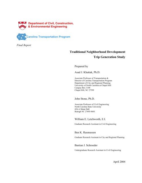
Traditional Neighborhood Development Trip Generation Study

Department of Civil, Construction, 

& Environmental Engineering 

Carolina Transportation Program 

Final Report 

Traditional Neighborhood Development 

Trip Generation Study 

Prepared by 

Asad J. Khattak, Ph.D. 

Associate Professor of Transportation & 

Director of Carolina Transportation Program 

Department of City and Regional Planning 

University of North Carolina at Chapel Hill 

Campus Box 3140 

Chapel Hill, NC 27599 

John Stone, Ph.D. 

Associate Professor of Civil Engineering 

North Carolina State University 

424-A Mann Hall 

Raleigh NC 27695-8601 

William E. Letchworth, E.I. 

Graduate Research Assistant in Civil Engineering 

Ben K. Rasmussen 

Graduate Research Assistant in City and Regional Planning 

Bastian J. Schroeder 

Undergraduate Research Assistant in Civil Engineering 

April 2004

Technical Report Documentation Page 

1. Report No. 

2. Government Accession No. 

…leave blank… 

NCDOT 2003-13 

4. Title and Subtitle 

Traditional Neighborhood Development Trip Generation 

Study 

7. Author(s) 

Asad Khattak & John Stone 

9. Performing Organization Name and Address 

Center for Urban & Regional Studies, Department of City and Regional Planning 

University of North Carolina at Chapel Hill, CB 3140, Chapel Hill, NC 27599 

3. Recipient’s Catalog No. 


5. Report Date 

January 2004 

6. Performing Organization Code 


8. Performing Organization Report No. 


10. Work Unit No. (TRAIS) 


Department of Civil, Construction and Environmental Engineering, Mann Hall, 

NC State University, Raleigh NC 27695 

12. Sponsoring Agency Name and Address 

North Carolina Department of Transportation 

Research and Analysis Group 

1 South Wilmington Street 

Raleigh, North Carolina 27601 

Supplementary Notes: 


11. Contract or Grant No. 


13. Type of Report and Period Covered 

Final Report 

July 1, 2002- December 31, 2003 

14. Sponsoring Agency Code 

NCDOT Project # 2003-13 

16. Abstract 

Since the beginning of the new urbanist movement, alternately referred to as Traditional Neighborhood 

Developments (TNDs), planners and architects have touted their neighborhood and community designs 

for reducing residents’ reliance on the automobile by creating compact, mixed use, and pedestrianfriendly 

developments. However, researchers have not explicitly examined how travel behavior and 

traffic impacts differ in a tightly controlled comparison of conventional and traditional developments. 

Additionally, current forecasting models and trip generation procedures need to be tested for their 

applicability to these new developments. This report aims to fill that void by studying a matched-pair of 

neighborhoods: One conventional and one traditional. The neighborhoods are located in the Chapel 

Hill/Carrboro area of North Carolina. Traffic counts were taken at all entrances and exits to the 

developments and a detailed behavioral survey of the residents was conducted in the two neighborhoods 

during 2003. The results show that households in Southern Village, the TND, make about the same 

amount of total trips, but significantly fewer automobile trips, fewer external trips and they travel fewer 

miles, when compared to households in the conventional neighborhoods. However, this reduction of trips 

in a suburban environment does little to decrease delay at “over-designed” intersections along major 

highways. Finally, ITE trip generation methods and rates are acceptable for predicting the trip generation 

of the study neighborhoods. The implications of these results are discussed in the report. 

17. Key Words 

Traveler behavior, traditional neighborhood 

developments, trip generation, vehicle miles traveled 

19. Security Classif. (of this report) 

Unclassified 

18. Distribution Statement 


20. Security Classif. (of this page) 

Unclassified 

21. No. of Pages 22. Price 


Form DOT F 1700.7 (8-72) 

Reproduction of completed page authorized

Disclaimer 

The contents of this report reflect the views of the authors and not necessarily the views of the 

University of North Carolina at Chapel Hill or North Carolina State University. The Authors are 

responsible for the facts and the accuracy of the data presented herein. The contents do not 

necessarily reflect the official views or policies of the North Carolina Department of 

Transportation or the Federal Highway Administration. This report does not constitute a 

standard, specification, or regulation. 

Acknowledgements 

We are very grateful to the chair and members of the NCDOT TND project committee (2003- 

13), who have provided very valuable input and data for the project. They are: 

• Harrison Marshall (Chair) 

• Jamal Alavi, PE 

• Tom Norman 

• Michael Penney 

• Loretta Barren 

• John Hodges-Copple 

• Bill McNeil 

• David Bonk 

• Moy Biswas, Ph.D., PE 

• Rodger Rochelle, PE 

• Derry Schmidt, PE 

• Daniel Holt 

UNC Acknowledgements 

Professor Daniel Rodriguez was a major contributor to the research project. Graduate students 

Ben Rasmussen, Steve Wernick, Jennifer Genzler, David Anspacher and undergraduate student 

Jennifer Valentine (University of North Carolina at Chapel Hill) worked on the project and were 

instrumental in the completion of this study. We are also very grateful to the NCDOT Research 

and Analysis Group for their support during the project. 

NCSU Acknowledgements 

The authors appreciate the contributions and hard work of staff at NCDOT and students at 

NCSU. We extend special thanks to the following persons who provided help and information 

throughout the project: Meredith Harris, Elizabeth Sall, George Small, Kumar Neppalli, Adam 

Snipes, Gary Faulkner, Jim Earnhardt, and Tim Padgett. Very special thanks are due to Kent 

Taylor of the NCDOT Traffic Surveys Unit for his help in obtaining traffic counts at the 

entrances to the study developments. 

ii

Executive Summary 

Introduction 

Traditional Neighborhood Developments (TNDs) are characterized by human-scale, walkable, 

and transit friendly communities with moderate to high densities and a mixed-use core. TNDs 

are becoming increasingly popular in the United States and North Carolina, and they are 

expected to encourage walking and bicycling and increase the percentage of trips performed 

inside the development, due to the mixture of land uses. 

Over the past decade, a number of Traditional Neighborhood Developments were completed in 

the Triangle Area. Examples include Southern Village and Meadowmont in Chapel Hill, and 

Carpenter Village in Cary. As these types of neighborhoods become increasingly popular, a 

closer assessment of the traffic impacts of TND designs becomes warranted. Conceptually, TND 

design encourages walking by decreasing distances to shops and businesses and creating a 

pleasant and safe neighborhood environment. Even without an increase in walking, TND designs 

intend to capture vehicular trips within neighborhood boundaries by providing amenities in the 

village centers, as well as, cause a mode shift towards public transportation, the implementation 

of which becomes more viable in a more denser development style. 

However, the differences in traveler behavior and the resulting effects on traffic of these 

developments are yet to be determined and scientific analyses are required to assess whether 

proclaimed benefits of the design are indeed occurring. Current forecasting models and trip 

generation procedures need to be tested for their applicability to these new developments. This 

research report assesses the impacts of a TND neighborhood by comparing trip generation and 

traffic impact analysis results to actual traffic counts taken at the neighborhood boundaries and 

by investigating the results of resident and business surveys taken in the Southern Village (TND 

neighborhood) and Northern Carrboro developments (conventional neighborhoods) near Chapel 

Hill North, Carolina. 

Project Scope and Objectives 

Traditional Neighborhood Developments (TNDs) are planned in a relatively high-density design 

and combine a mix of land uses within the boundaries of the development. Chapter 7 of the 

Institute of Transportation Engineers (ITE) Trip Generation Handbook defines Multi-Use 

Developments as “typically a single real-estate project that consists of two of more ITE land use 

classifications between which trips can be made without using the off-site road system”. 

Southern Village, a development south of Chapel Hill, NC was designed in the style of TNDs 

and fits the ITE definition of multi-use development because it contains houses, shops, 

restaurants, a grocery store, a movie theatre, offices, a day care center, and a an elementary 

school within its boundaries. 

For comparative purposes, a second residential area was chosen, which was not designed in the 

style of TNDs. The Northern Carrboro neighborhoods, also near Chapel Hill, NC, were selected 

because they were determined to best represent the opposite side of the spectrum in relation to 

Southern Village with respect to factors that might influence the number of trips people make 

iii

and how likely people are to use walking, biking or transit for trips. These factors include: mix 

of uses, density or “compactness” of development, availability/quality of pedestrian and bike 

features (sidewalks, bike lanes, etc.), availability/quality of transit service, street connectivity, 

site design/layout features, and proximity to destinations. By choosing the Northern Carrboro 

neighborhoods, we get to see two ends of the spectrum on these related factors for what are 

expected to be similar demographic groups, thus any differences in travel behavior should 

represent two endpoints. 

By comparing Southern Village with Lake Hogan Farms (a conventional development within the 

Northern Carrboro neighborhoods), we can compare differences in trip generation and actual 

traffic volumes for one example of each development form. In this study, only these two 

neighborhoods were assessed and all results are only proven to be applicable for these two 

examples. Generalizations for other TNDs in North Carolina or nationwide, therefore have to be 

treated with care. 

TNDs are expected to encourage the use of alternative modes, and increase internal trip capture 

rates ultimately reducing congestion, vehicle miles traveled and to improve air quality. The 

behavioral trip generation portion of this study assesses if indeed trip generation rates and 

alternative mode use are any different in Southern Village compared with more conventional 

developments in Northern Carrboro. The study conducted a resident survey of Southern Village 

TND and Northern Carrboro conventional neighborhoods (N=453 households) and also collected 

spatial data on the developments. In addition, data regarding trips to on-site commercial and 

retail offices in the Southern Village TND was collected to understand the travel characteristics 

of office and retail users. The study survey attempts to distinguish between trip types, such as 

home-based-work or home-based-other, and to estimate the effects of TND design such as trip 

chaining, mode choice, internal capture, and pass-by trips. 

For the two neighborhoods, typical traffic impact analysis (TIA) methods were also utilized to 

explore TND trip generation. Traffic generation was performed using the methods developed by 

ITE, as well as, spreadsheet implementations of these methods developed by a consultant. As an 

additional method to explore trip generation the study used the Triangle Regional Travel 

Demand Model to obtain further trip estimates. It was not the objective of this study to develop 

new methods for traffic forecasting, but rather to apply, verify and validate existing ones. In that 

regard all traffic generation estimates were compared to traffic counts taken on streets 

entering/exiting the neighborhood. 

The focus of the traffic generation portion of this study is on the total site traffic generated and 

overall volumes counted at the entrances and exits to the developments. The study did not look at 

internal distribution and did not distinguish between trip types, such as home-based-work or 

home-based-other. Other proclaimed features and effects of TND design such as trip chaining, 

mode choice, internal capture, and pass-by trips are discussed in the literature review, and are 

analyzed in the traffic generation portion of the document to the extent that they affect the total 

traffic volumes entering and exiting the neighborhood. The traffic generation estimates and 

methods reflect and validate current practice of consultants and public agencies. 

iv

Conclusions 

In terms of traveler behavior this study finds no statistically significant difference between the 

total trips made by households in the Southern Village TND and the comparable conventional 

developments. However, TND households substituted driving trips with alternative modes, i.e., 

the automobile trip generation rate for the TND was significantly lower (by 1.25 trips per day per 

household) than conventional neighborhoods. In addition, empirical evidence suggests that TND 

households have: 

• Lower vehicle miles traveled—on average, the TND single-family households travel 18 

miles less per day. 

• Higher share of alternative modes—in the TND, 78.4 percent of the trips were by 

personal vehicle compared with 89.9 percent in the conventional neighborhoods. 

• Lower external trips—on average, the TND households made 1.53 fewer external trips 

per day. 

The TND examined in this study internally captured a substantial share of the total trips 

produced (20.2 percent). By comparison, the conventional neighborhoods internally captured a 

much smaller share of the total trips (5.5 percent). Therefore the difference between the internal 

trip capture rates for the two development types is 14.7 percent. 

The Southern Village TND business survey asked business managers about their employees and 

customers/visitors. It revealed that only 5.2 percent of the 432 employees reside in Southern 

Village and a large majority of the employees (92.4 percent) use personal vehicles to commute to 

work. This is not surprising given the free employee parking in Southern Village and relatively 

high levels of automobile ownership by people who work. A significant percentage of 

customers/visitors (39.2 percent) reside in Southern Village; about 18.1 percent of the total trips 

attracted to Southern Village businesses are reportedly by walking. The results show that 

Southern Village employees use passenger cars as often as employees in conventional facilities, 

but that customers/visitors are more likely to walk. Off-site employees and customers/visitors 

make up a majority of trips attracted to the TND businesses. 

Examination of the ITE methods for trip generation, and comparison of trip generation results to 

counts taken at both Southern Village and Lake Hogan Farms, verify the ITE methods for trip 

generation for mixed-use and conventional neighborhoods. The Triangle Regional Model was 

too aggregate to study single neighborhoods. A study of the micro-simulation VISSIM and other 

simulation models shows that such simulations hold promise for single neighborhood analysis, 

particularly with respect to internal vehicle and pedestrian circulation. 

A sensitivity analysis of the affect of internal capture on access traffic indicated that the 

reduction in vehicle trips due to the internal capture of Southern Village does not significantly 

improve the level of service of the intersections adjacent to the development, even during the 

peak hour. A development located in a more urban area may have larger internal capture effects 

due to the greater interconnectivity of surface streets and an increase in the number of shopping 

and work opportunities available to the residents of the area. 

v

Table of Contents 

Chapter 1: Introduction................................................................................................................1-1 

Problem............................................................................................................................1-1 

Scope and Definition of Terms for Travel Behavior .......................................................1-2 

Scope and Objectives for Trip Generation.......................................................................1-3 

Chapter Summary ............................................................................................................1-4 

Chapter 2: Literature Review.......................................................................................................2-1 

Introduction......................................................................................................................2-1 

TND Design Issues and Resident Travel Behavior .........................................................2-1 

TND Issues Related to Traffic Impact Analyses .............................................................2-4 

Traffic Impact Analysis Methods Applicable to TNDs...................................................2-7 

Synopsis of Methods for Traffic Impact Analysis...........................................................2-8 

Chapter Summary ..........................................................................................................2-12 

Chapter 3: Methods for Traveler Behavior..................................................................................3-1 

Hypotheses.......................................................................................................................3-1 

Description of Neighborhoods.........................................................................................3-2 

Sampling ..........................................................................................................................3-5 

Survey Design..................................................................................................................3-5 

Data Files .........................................................................................................................3-8 

Socioeconomics ...............................................................................................................3-9 

Chapter 4: Analysis and Findings for Traveler Behavior ............................................................4-1 

Descriptive Analysis ........................................................................................................4-1 

Estimation of Trip Generation Models ..........................................................................4-17 

TND Travel Behavior Models .......................................................................................4-29 

Business Trip Generation Rates.....................................................................................4-32 

Chapter 5: Research Approach for Trip Generation....................................................................5-1 

Introduction......................................................................................................................5-1 

ITE Method.....................................................................................................................5-1 

Discussion and Critique of the ITE Trip Generation Method..........................................5-4 

Travel Demand Model .....................................................................................................5-5 

Discussion and Critique of the Travel Demand Model ...................................................5-8 

Components of Resident Survey......................................................................................5-9 

Collection of Traffic Counts ............................................................................................5-9 

Discussion and Critique of Count Method.....................................................................5-11 

Chapter Summary ..........................................................................................................5-12 

Chapter 6: Analysis of Case Studies............................................................................................ 6-1 

ITE Trip Generation.........................................................................................................6-1 

Triangle Regional Model Trip Generation ......................................................................6-4 

Neighborhood Survey Trip Generation ...........................................................................6-4 

Comparative Results and Discussion............................................................................... 6-5 

vii

Sensitivity Analysis .........................................................................................................6-9 

Sensitivity Analysis Summary.......................................................................................6-13 

Feasibility of Traffic Simulation Methods.....................................................................6-15 

Conclusions.................................................................................................................... 6-15 

Chapter 7: Summary Findings, Conclusions and Recommendations..........................................7-1 

Traveler behavior: Trip Generation .................................................................................7-1 

Traveler Behavior: Limitations........................................................................................7-3 

Traveler Behavior: Recommendations ............................................................................7-3 

Traffic Analysis: Trip Generation....................................................................................7-4 

Traffic Analysis: Methods ...............................................................................................7-4 

Traffic Analysis: Impacts of Neo-Traditional Developments .........................................7-5 

Traffic Anlysis: Implications for Neighborhood Development.......................................7-5 

Traffic Study: Conclusions ..............................................................................................7-6 

Traffic Study: Recommendations ....................................................................................7-7 

APPENDICES ............................................................................................................................... A 

Appendix A: Relevant studies, their location, sample, and independent variables....... A-1 

Appendix B: Process for selecting the neighborhoods used in this study..................... B-1 

Appendix C: Income Response Rates by Neighborhood .............................................. C-1 

Appendix D: Means of responses to attitudinal questions by neighborhood type ........ D-1 

Appendix E: Southern Village Business Survey Report................................................E-3 

Appendix F: Targa, F. 2002. “Final Paper: Trip Generation – Land Use.”...................F-1 

Appendix G: Survey instrument and travel diary used in this study............................. G-1 

Appendix H: Survey Variables...................................................................................... H-1 

Appendix I: Selected Modeling Results.........................................................................I-1 

Appendix J: Neighborhood Descriptions ...................................................................... J-1 

Appendix K: Sample ITE Trip Generation Spreadsheets.............................................. K-1 

Appendix L: Southern Village ITE Trip Generation .....................................................L-1 

Appendix M: Triangle Regional Model Socio-economic Data .................................... M-1 

Appendix N: Signal Timing and Traffic Counts ........................................................... N-3 

Appendix O: Sensitivity Analysis Discussion............................................................... O-1 

Appendix P: Sensitivity Analysis Tables.................................................................... PR-1 

Appendix Q: Resident Survey ....................................................................................... R-1 

Appendix R: Simulation................................................................................................ R-1 

viii

List of Figures 

Figure 3-1: Location of Northern Carrboro and Southern Village ..............................................3-3 

Figure 3-2: Distribution of Households Sampled ........................................................................3-6 

Figure 3-3: Household Survey Conceptual Structure .................................................................3-7 

Figure 3-4: Location of Households that Completed TND Survey .............................................3-9 

Figure 4-1: Comparative Household Income ..............................................................................4-2 

Figure 4-2: Start Time of Trips....................................................................................................4-5 

Figure 4-3: Trips by Mode by Neighborhood............................................................................4-12 

Figure 4-4: External and Internal Trips by Mode Share............................................................4-12 

Figure 4-5: Trip Type by Neighborhood ...................................................................................4-13 

Figure 4-6: Trips by Mode by Type (Southern Village)............................................................4-14 

Figure 4-7: Trips by Mode by Type (Northern Carrboro) ......................................................... 4-14 

Figure 4-8: Trip Distance by Mode (Southern Village).............................................................4-15 

Figure 4-9: Trip Start Times by Mode -- Southern Village.......................................................4-15 

Figure 5-1: Research Approach ...................................................................................................5-1 

Figure 5-2: ITE Trip Generation Model ......................................................................................5-2 

Figure 5-3: TRM Trip Generation Method................................................................................5-25 

Figure 5-4: Traffic Count Locations for Southern Village ........................................................5-10 

Figure 5-5: Traffic Count Locations for Lake Hogan Farms.....................................................5-11 

Figure 6-1: Sensitivity Analysis Summary................................................................................6-14 

List of Tables 

Table 2-1: TND Modeling Capabilities of TIA Methods ..........................................................2-13 

Table 3-1: Hypotheses Tested......................................................................................................3-2 

Table 3-2: Density, Diversity and Design Characteristics of Our Study Sites ............................3-3 

Table 3-3: Additional Characteristics of Our Study Sites ...........................................................3-4 

Table 3-4: Response Rates...........................................................................................................3-5 

Table 4-1: Assessed Housing Values of the Population ..............................................................4-3 

Table 4-2: Number of People and Cars in Household .................................................................4-4 

Table 4-3: Number of Total Trips and Car Trips per Household ................................................4-4 

Table 4-4: Tours and Stops per Household..................................................................................4-6 

Table 4-5: Daily Length of Trips per Household in Time and Distance .....................................4-8 

Table 4-6: Regional Trips (> 10 miles) per Household per Day .................................................4-9 

Table 4-7: Variable Means at the Person Level – Residents of Single Family Homes .............4-10 

Table 4-8: External Trips and External Trip Duration and Distance per Household per Day...4-10 

Table 4-9: Trips by Mode by Neighborhood .............................................................................4-11 

Table 4-10: Trip Type per Neighborhood..................................................................................4-13 

Table 4-11: Physical Activity Trips by People by Neighborhood.............................................4-16 

Table 4-12: Trip generation model of the Triangle ...................................................................4-17 

Table 4-13: Trip Generation Models .........................................................................................4-19 

Table 4-14: Trip Generation Models (Single-Family Homes) ..................................................4-21 

Table 4-15: External Trip Generation Models (Single-Family Homes)....................................4-22 

Table 4-16: Auto Trip Generation Models (Southern Village) .................................................4-24 

ix

Table 4-17: Auto Trip Generation Models (Northern Carrboro)............................................... 4-25 

Table 4-18: Trip Distance Models for Southern Village (miles)...............................................4-26 

Table 4-19: Trip Distance Models for Northern Carrboro (miles) ............................................4-27 

Table 4-20: Trip Duration Models for Southern Village (hours) ..............................................4-28 

Table 4-21: Trip Duration Models for Northern Carrboro (hours)............................................4-28 

Table 4-22: Regression Models for Auto Trips .........................................................................4-30 

Table 4-23: Trip Distance Models (miles).................................................................................4-31 

Table 4-24: Trip Duration Models (hours) ................................................................................4-31 

Table 4-25: Physical Activity Trip Generation, Duration and Distance Models.......................4-32 

Table 4-26: Southern Village employers, their size, and their number of employees...............4-33 

Table 5-1: TRM Trip Generation Urban Cross-Class Matrices...................................................5-7 

Table 6-1: Southern Village ITE Trip Generation (No Internal Capture) ...................................6-1 

Table 6-2: Southern Village Daily Internal Capture Results.....................................................6-12 

Table 6-3: Southern Village PM Peak Hour Internal Capture Results ........................................6-2 

Table 6-4: Southern Village November 2002 Trip Generation ...................................................6-3 

Table 6-5: Lake Hogan Farms March 2003 Trip Generation ......................................................6-3 

Table 6-6: TRM Trip Generation Estimates ................................................................................6-4 

Table 6-7: Southern Village Resident Survey Trip Estimates (2003) .........................................6-4 

Table 6-8: Lake Hogan Farms Resident Survey Trip Estimates..................................................6-4 

Table 6-9: Southern Village Daily Trip Generation Comparison..............................................6-45 

Table 6-10: Southern Village PM Peak Trip Generation Comparison........................................6-6 

Table 6-11: Lake Hogan Farms Daily Trip Generation Comparison ..........................................6-6 

Table 6-12: Lake Hogan Farms PM Peak Trip Generation Comparison.....................................6-7 

Table 6-13: Comparison of Survey and ITE Trip Generation, Southern Village........................6-7 

Table 6-14: Comparison of Survey and ITE Trip Generation, Lake Hogan Farms ....................6-8 

Table 6-15: Summary of Southern Village Trip Generation .......................................................6-8 

Table 6-16: Summary of Lake Hogan Farms Trip Generation....................................................6-9 

Table 6-17: Variability of ITE Trip Generation Rates...............................................................6-10 

Table 6-18: Capacity Analysis for Percent Increases in Traffic Volumes.................................6-11 

Table 6-19: Comparison of Different Land Use Types .............................................................6-11 

Table 6-20: Effect of Internal Capture Rate on Capacity Analysis ...........................................6-12 

Table 6-21: Volume Comparison for Main Street/US15-501....................................................6-12 

x

Chapter 1: Introduction 

This report presents the findings of a study on travel behavior and trip generation associated with 

a traditional neighborhood development (TND) and how TND travel characteristics are different 

from those in a nearby conventional suburban development. The Department of City and 

Regional Planning of the University of North Carolina at Chapel Hill and the Department of 

Civil, Construction, and Environmental Engineering at North Carolina State University 

completed the research for the North Carolina Department of Transportation (NCDOT). While 

the UNC-Chapel Hill team focused on resident and business surveys and the travel behavior of 

the residents of the neighborhoods, the N.C. State team concentrated on trip generation 

procedures, vehicle counts leaving the development, and traffic impacts on adjacent streets. 

Problem 

The number of neighborhood-scale new urbanist projects completed or under construction rose 

37 percent between 2000 and 2001 and has risen by 20 percent or more per year over the past 

five years. 1 An estimated 1.4 million people reside in new urbanist communities (Berke et al. 

2003). More than half of these projects were built on Greenfield sites. Such neighborhoods are 

emerging in North Carolina, and in fact, North Carolina Department of Transportation (NCDOT) 

has issued guidelines for designing Traditional Neighborhood Developments (TNDs). Over the 

past decade, a number of TNDs have been completed in the Research Triangle Area. Examples 

include Southern Village and Meadowmont in Chapel Hill, Carpenter Village in Cary, and North 

Hills in Raleigh. Unlike the conventional development practices of the 1970s and 1980s, typified 

by single-use, large lot residential developments with strip commercial centers located on the 

periphery and businesses located in separate business parks, new urbanist/traditional community 

design stresses a mix of uses compactly arranged in a single development. Planning theorists 

believe that individuals rely on automobiles to travel from place to place in conventional 

communities because each land use, such as residential, commercial, and business, is separated 

and spread out. When pedestrian-oriented design features such as continuous sidewalks and 

street trees are combined with the mixed land uses typically found in traditional communities, 

individuals should theoretically drive less and walk more. To investigate this hypothesis, the 

following report explores the impacts of a TND on trip production and attraction, mode choice, 

and trip chaining by comparing and analyzing the differences in travel behavior between a 

conventional neighborhood, a TND, and the Triangle region (Raleigh-Durham-Chapel Hill). One 

fundamental research question that we will attempt to answer is: Do residents of TNDs in North 

Carolina have lower trip generation rates, automobile use and vehicle miles traveled compared 

with more conventional, auto-oriented neighborhoods 

Additionally, as these types of neighborhoods become increasingly popular, a closer assessment 

of traffic impacts caused by TND designs becomes warranted. The TND development form is a 

fairly new design concept, and there are few existing TNDs in North Carolina upon which to 

base trip generation and traffic forecasts. Trip generation and traffic impact analysis methods that 

are commonly used for new suburban neighborhoods may or may not be appropriate for TND 

traffic impact analyses. It is essential, however, for traffic forecasting and trip generation 

1 These projects are greater than 15 acres. Source: New Urban News, 2001, “New urbanist project construction 

starts soar.” http://www.newurbannews.com/annualsurvey.html 

1-1

professionals to obtain reliable estimates of traffic volumes resulting from a new TND plan in 

order to develop street access and have the plan approved by local officials. 

Without reliable forecasting techniques, disputes may arise for a new TND. Developers may 

claim reduced TND traffic impacts while city officials seek mitigation for the TND traffic 

generated. Furthermore, if the TND access uses state roads, NCDOT must review and approve 

the TND plan. Thus, it is essential for NCDOT to have a reliable method to substantiate TND 

traffic impact analyses. 

This research report assesses impacts of a TND neighborhood by comparing trip generation and 

traffic impact analysis results to actual traffic counts taken at the neighborhood boundaries. The 

study includes one neighborhood that meets TND standards and one neighborhood that is 

designed in a conventional single-use suburban design. 

Scope and Definition of Terms for Travel Behavior 

Before proceeding further, we will define and discuss a number of key terms. A trip is defined 

as the movement of a person in space (at least 300 feet) and time. In this study we focus on daily 

trips, which are mostly done within a city/region, i.e., the trips studied are less than 100 miles. 

The two neighborhood types that were surveyed in the study had distinctly different land use 

characteristics and their boundaries were clearly defined, e.g., Southern Village is a TND, with 

residents having a fairly clear idea of the shape and size of the development. We will refer to 

new urbanist, neotraditional neighborhoods as traditional neighborhood developments. 

Trip generation is composed of both trip productions and trip attractions. We analyze residential 

trip productions and the trips analyzed include bicycling and walking modes. The trip purposes 

analyzed included: Home-based work, home-based shop, home-based school, home-based other, 

and non-home-based. While trip production is expressed as a function of socio-economic data 

and/or population at the household level, such as household size, number of cars present, and 

household income, trip attraction is expressed as function of land use, employment, and/or other 

economic activities such as shopping and entertainment destinations. As part of our study, we 

will estimate trip generation models to quantify and compare trip generation rates across 

traditional and conventional neighborhoods and also compare them with the larger Triangle 

region trip generation rates. This study also explores trip attractions in the TND by surveying the 

businesses. 

Mode choice is an individual’s selection from a variety of transportation options, including 

private vehicle, bus, walking, and bicycling. It is most often a function of time, cost and 

socioeconomic variables; and of course it depends on the availability of alternatives. For 

instance, an individual may choose to drive because their destination is far away, they need to 

transport people or goods, and/or there are no alternatives, such as public transportation. 

Conversely, a person may choose to walk when their destination is nearby, they are not 

transporting other people or goods, and/or there is a network of sidewalks and trails connecting 

them to their destination. More intangible, however, is the appeal of using various modes of 

transportation. For instance, some people may prefer driving because of the freedom this choice 

permits, while other people prefer riding the bus so they can work while they commute. This 

1-2

study will examine mode choice within the framework trip generation, i.e., number of 

automobile trips that are generated. 

Trip chaining is another component of trip generation and is defined as the process of making a 

series of non-home based trips in a row. Trip chaining is composed of stops and each chain of 

stops is known as a tour. An example of trip chaining is running errands, which is more 

convenient for single occupant automobile users than for carpoolers or transit users. Trip 

chaining is generally considered more efficient than returning home after each destination is 

reached. However, the distribution and distance of the destinations should be considered before 

such conclusions can accurately be made. For instance, it may be more efficient to chain trips 

when the origination is located far from destinations and/or when the destinations are clustered in 

one or a few areas, away from the origination of the trip. However, it may not necessarily be 

efficient to chain trips when alternative modes, such as transit or walking, are available, the 

origination is close to the destinations and the destinations are spread out around the origination. 

Regardless, many people may choose to chain trips once they have begun running errands 

despite what may be most efficient. Because trip chaining has not been thoroughly studied, this 

study attempts to understand trip chaining in the traditional versus conventional context. 

Scope and Objectives for Trip Generation 

The objective of this portion of the study is to determine the reliability of currently accepted 

traffic forecasting methods, not to develop new methods. The focus of this report is on the total 

site traffic generated and the traffic volumes at the entrances and exits to Southern Village 

(TND) and Lake Hogan Farms (conventional suburban development, or CSD) in Chapel Hill, 

NC. The specific objectives of the study are: 

• To estimate, count, and compare site traffic at a TND and a CSD using conventional 

traffic impact analysis (TIA) and travel demand model (TDM) methods 

• To compare TND and CSD trip rates implied from travel diaries to published trip rates, 

including internal capture rates 

• To recommend changes (if any) in NCDOT traffic impact analysis methods and TDM 

methods to address the specific travel impacts of TNDs 

Chapter 7 of the ITE Trip Generation Handbook defines multi-use developments as “typically a 

single real-estate project that consists of two or more ITE land use classifications between which 

trips can be made without using the off-site road system” (ITE, 2001). Southern Village was 

designed as a TND and fits the ITE definition of a multi-use development. The Southern Village 

area contains houses, shops, restaurants, a grocery store, a movie theatre, offices, a day care 

center, and an elementary school within its boundaries. 

For comparative purposes, a conventional suburban development (CSD) was studied. Lake 

Hogan Farms was selected as the comparison neighborhood because it is similar to the size, 

location, and demographics of Southern Village. However, such factors as mix of land uses, 

density or “compactness” of development, availability/quality of pedestrian and bike features 

(sidewalks, bike lanes, etc.), availability/quality of transit service, street connectivity, site 

design/layout features, and proximity to destinations are quite different from Southern Village. 

1-3

By comparing these two neighborhoods that share similar demographic groups but have different 

design elements, it is possible to compare trip generation and actual traffic volumes for each type 

of development. This study should yield significant insight into the trip generation 

characteristics of TNDs but generalizations for other TNDs in North Carolina or nationwide 

must be treated with care, due to the location and relative youth of the Southern Village 

development in comparison to older developments that may have the same retail and commercial 

opportunities but are more integrated into the urban fabric. 

Typical traffic impact analysis (TIA) methods were utilized for both neighborhoods. Trip 

generation was performed using the methods developed by ITE and implemented in 

spreadsheets. The study used the travel demand model (TDM) “Triangle Regional Model” to 

obtain additional trip estimates for further comparison 

Chapter Summary 

This chapter gave an overview of the project. Various problems related to TNDs were 

highlighted and the cope and objectives of this study were determined. Various terms related to 

trip making were also defined. 

1-4

Chapter 2: Literature Review 

Traffic Impacts and Assessment Methods For Traditional Neighborhood Developments 

Introduction 

In the 1990’s, a planning movement known as “The New Urbanism” led to the design and 

construction of a new category of neighborhoods across the nation. These “Neotraditional 

Neighborhood Developments” create more livable mixed land-use communities that promote 

walking and bicycle use, thereby reducing traffic congestion and related impacts. They feature 

compact residential development combined with additional land-uses like retail, office, and 

recreational facilities in a grid-pattern street design. The term “neotraditional” refers to the 

revitalized idea of the pre-World War II “traditional” design of closely connected, higher density 

urban neighborhoods, that preceded the 1950’s trend of “suburban” neighborhood developments. 

In this review, the term “traditional neighborhood development” (TND) will be used. TND 

examples in North Carolina include Falls River in Raleigh, Carpenter Village in Cary, and 

Meadowmont and Southern Village in Chapel Hill. Street and land-use design concepts for such 

TNDs are available to planners, engineers and architects. Relatively few U.S. researchers have 

attempted to determine how effective the neotraditional street and land-use designs really are in 

reducing traffic impacts compared to conventional suburban developments. Studies for North 

Carolina TNDs do not exist. This literature review examines TND features, particularly related 

to resident travel behavior and traffic issues, and evaluates alternative methods to estimate traffic 

impacts caused by these types of neighborhoods. 

TND Design Issues and Resident Travel Behavior 

This section provides a summary of the literature and identifies gaps in the literature. While the 

relationship between design and travel behavior has been studied broadly for large areas, it has 

not been studied specifically on the neighborhood scale for actual traditional neighborhoods. As 

the following literature shows, not only have the study areas been much larger and more difficult 

to define than actual neighborhoods, but studies have used traditional neighborhoods as a proxy 

for traditional neighborhoods primarily because few “mature” traditional neighborhoods exist 

(Crane, 1996; Cervero, 1995). However, this substitution is often not justifiable because 

(neo)traditional neighborhoods are often constructed on undeveloped areas on the fringe of city 

limits, whereas traditional neighborhoods, usually defined as neighborhoods built prior to World 

War II, are well-integrated into the urban fabric of the city as subsequent development has 

occurred around these neighborhoods. Additionally, some studies have found that income levels 

in traditional neighborhoods are lower than in more auto-oriented areas (Cervero, 1996), while 

this is not always the case for residents of (neo)traditional neighborhoods. Finally, many of the 

findings of the studies that examine the relationship between travel behavior and urban form may 

be applicable for the area where the studies were conducted, mainly in highly-urbanized regions 

of California, but are not applicable to other areas of the country. For these reasons and in the 

context of the current breadth of literature, we feel that the findings of our study will help 

broaden the understanding of the relationship between travel behavior and urban form and will 

be more useful in considering future traditional developments in North Carolina. 

2-1

First, it is necessary to look at the existing literature on the topic. A number of studies have 

broadly examined the impact of community form on travel behavior (Appendix A). 2 Using 

factor analysis, Cervero and Kockelman (1997) found that density, diverse land-uses, and 

pedestrian-oriented design dimensions of the built environment encourage non-auto travel in 

marginally statistically significant ways that differed between trip purposes and modal choice: 

compact development had the strongest influence on personal business trips, withinneighborhood 

retail shops had the strongest influence on mode choice for work trips, and people 

living in neighborhoods with grid street designs and restricted commercial parking averaged 

significantly fewer vehicle miles of travel and relied less on single-occupant vehicles for nonwork 

trips. 

Because urban form has the potential to increase walking and therefore physical activity rates, a 

number of public health related studies have been undertaken on the topic. Two such studies 

illustrate the type of work being done in the public health field. Craig et al. (2002) studied the 

effect of the physical environment on physical activity by rating eighteen neighborhood 

characteristics and correlating the scores with walking to work, as reported by households in the 

Canadian census. Though some of the characteristics could have been rated subjectively, they 

found that characteristics associated with traditional design, including density and the presence 

of mixed land uses, were correlated with walking to work. In a national study of the relationship 

between walking and urban form, Berrigan and Troiano (2002) found that people who lived in 

urbanized areas in homes built prior to 1946 and between 1946 and 1973 were significantly more 

likely to walk than people living in homes built after 1973. They argue that home age is a useful 

proxy for neighborhood design; however the designs of neighborhoods built between 1946 and 

1973 vary greatly and are not always consistent with neighborhoods built before 1946. 

On the transportation and city planning side of the neighborhood design, Ewing and Cervero 

(2001) recently conducted a seminal literature review of the topic. With respect to 

neighborhood/activity center design impacts on travel behavior, many of the cases they reviewed 

used traditional neighborhoods as a proxy for neotraditional neighborhoods and were mainly set 

in California. Additionally, the conventional neighborhoods used in those studies were built 

anytime between the end of World War II and present day. The authors found that trip 

frequencies depend mainly on household socioeconomic characteristics and that travel demand is 

inelastic with respect to accessibility. Trip frequencies are therefore a secondary function of the 

built environment. 

Ewing and Cervero (2001) also found that walking is more prevalent and that trip lengths are 

generally shorter in traditional urban settings. While trip lengths are primarily a function of the 

built environment and secondarily a factor of socioeconomic characteristics, mode choices 

depend on both, though perhaps less so on the built environment. With respect to the prevalence 

of walking, Ewing and Cervero (2001) make two important points. First, the prevalence of 

walking may be due to a self-selecting process, that is to say that people who like to walk choose 

to live in neighborhoods with a supportive walking environment. Second, it is unclear as to 

whether walking trips in traditional neighborhoods substitute or supplement longer automobile 

trips. However, the findings of at least two studies (Cervero and Radisch, 1996; Handy 1996) 

support the substitution possibility. 

2 Handy et al (2002) recently identified over 70 such studies in just the 1990s. 

2-2

In most instances, these studies involve the use of travel behavior data over large urban areas or 

multiple neighborhood sites. While travel behavior data usually come from metropolitan travel 

surveys, neighborhood data are extracted from census tract information or local land use 

inventory databases and are sometimes supplemented with neighborhood surveys created by the 

authors of the study. These approaches are fraught with difficulties. Travel behavior data from 

metropolitan surveys rarely yield enough observations per census tract; therefore, tracts are often 

combined. These methods may not adequately represent neighborhoods, as single or multiple 

census tracts rarely follow or capture neighborhood boundaries (Crane and Crepeau, 1998). 

Additionally, neighborhood environmental data is usually separated into multiple attributes, such 

as sidewalk width, social dynamics, four-way intersection frequency, street layout (grid vs. 

curvilinear), mix of uses, population density, job density, the presence of other people, and visual 

interest. In line with Cervero (1993), design elements, such as sidewalk width or presence of 

street trees “are too ‘micro’ to exert any fundamental influences on travel behavior.” 

Additionally, not only are some of these attributes, such as “visual interest” or “ease of street 

crossing”, difficult to measure objectively and/or consistently (Handy et al., 2002; Ewing and 

Cervero, 2001), but the multicolinearity and statistical interaction between the attributes render 

many of the built environment variables statistically insignificant. 3 

Each of the attributes mentioned above can be grouped into what Cervero refers to as the ‘3-Ds’: 

density, diversity, and design. While density may be relatively easy to measure, diversity and 

design elements typically are not. Cervero and Kockelman (1997) correctly note that it is the 

synergy of the 3-Ds in combination that is more likely to yield appreciable impacts with regard 

to travel behavior. Instead of attempting to determine the impact of each neighborhood attribute 

or to use complicated factor analysis that results in multiple, difficult to interpret variables 

(Ewing and Cervero, 2001), neighborhood qualities are best identified as a whole. In this 

manner, we can best capture the interaction between the 3-Ds. 

As in the design of this study, Cervero and Radisch (1996) use a matched-pair comparison of 

two neighborhood types in the San Francisco Bay Area to measure the impact of the synergy of 

the 3-Ds. They found that the compact, mixed-use, and pedestrian-oriented nature of a 

traditional neighborhood resulted in a significantly lower share of automobile trips. These trips 

were replaced by a higher share of walking and transit trips compared to the trips made in a 

conventional neighborhood. 

While Cervero and Radisch’s (1996) study is rightly criticized for failing to isolate the effects of 

different elements of urban design on travel behavior and their magnitudes (Ewing and Cervero, 

2001; Crane and Crepeau, 1998; Handy, 1996), we believe it is a simple and effective way to 

gauge the overall impact of such developments on travel behavior. Past studies have attempted 

to tease out the individual effects of various design elements with limited success. Unfortunately, 

few elements are found to be statistically significant influences in multiple studies (Boarnet and 

Crane, 2001) and some are regarded as spurious (Ewing and Cervero, 2001). Hypothetically, 

even if such elements were consistently identified, the utility of such findings would be 

debatable, as planners and developers who then incorporated statistically significant elements 

3 Cervero and Kockelman (1997) 

2-3

into their designs (such as street trees) and ignored statistically insignificant elements (such as 

having continuous sidewalks) may yield little change in travel behavior (in this case, walking). 

Though their methodology is similar to our study, significant differences exist. Whereas Cervero 

and Radisch used two neighborhoods built before and after World War II in their study – 

Lafayette as a conventional suburban neighborhood and Rockbridge as a proxy for a neotraditional 

neighborhood – we use new neighborhoods built in the last decade – the northern 

Carrboro neighborhoods (Lake Hogan Farms, Wexford, Fairoaks, Sunset Creek, and the 

Highlands) as conventional suburban neighborhoods and Southern Village as an actual neotraditional 

neighborhood. A number of other studies have used traditional neighborhoods as a 

proxy for neotraditional neighborhoods. 4 By using an actual neotraditional neighborhood in our 

study, we are able to control for the age of the development with respect to its more conventional 

counterpart and we are better able to represent the travel behavior impacts of proposed and 

existing traditional neighborhoods. 

Though the neighborhoods Cervero and Radisch used contain a similar mix of elements to those 

of our neighborhoods (Lafayette and the northern Carrboro neighborhoods are primarily single 

use neighborhoods with homes placed on large lots and Rockbridge and Southern Village are 

denser, mixed-use neighborhoods), noticeable differences exist. First, Lafayette and Rockbridge 

are larger than the northern Carrboro neighborhoods and Southern Village. Additionally, 

because these neighborhoods are older, they are also surrounded by development, while the 

northern Carrboro neighborhoods and Southern Village are located on the fringe of the city 

limits. Additionally, Lafayette has a commercial corridor while the northern Carrboro 

neighborhoods do not. Both Bay Area neighborhoods have rail (BART) stations near their 

commercial districts while only Southern Village is served by bus transit. Finally, Handy (1996) 

correctly notes that, “the findings of the numerous West Coast studies, especially those in the 

Bay area, may not prove to be fully generalizable to other parts of the U.S.” due to such 

differences as urban form, culture, and topography. Our study is the first of its kind in this area 

of the country and will broaden our understanding of how travel patterns may differ in various 

geographic regions. Overall, while Lafayette and Rockbridge best capture the differences in 

travel behavior between older, larger, transit-served neighborhoods that are more integrated into 

urban areas, the northern Carrboro neighborhoods and Southern Village best capture the 

differences in travel behavior between new, smaller, less transit-oriented developments that are 

less integrated into urban areas. While not typical of all new development, the northern Carrboro 

neighborhoods and Southern Village do represent the types of neighborhoods being proposed 

and built in many areas of North Carolina (e.g., Afton Village, Vermillion and Cheshire) and the 

rest of the country. 

TND Issues Related to Traffic Impact Analyses 

In the early 1990’s, around the time when the first neotraditional neighborhoods were being 

constructed, several studies attempted to predict the effect of the new land-use design on 

vehicular traffic by comparing hypothetical models of traditional neighborhood developments 

(TND) to conventional suburban developments (CSD). Cevero and Landis (1995) concluded in 

their study that land-use could be an important contributor to transportation trends and vice 

4 Dozens of such studies exist; see Ewing and Cervero (2001) for a listing. 

2-4

versa. Stone, Foster and Johnson (1992) examined two hypothetical street designs and found that 

TND land-use strategies would lead to a significant reduction in vehicle miles traveled (VMT) 

for a 5%-15% transit/pedestrian modal split compared to a suburban neighborhood; even with 

100% automobile travel, the TND would still reduce VMT, though marginally. Additional 

infrastructure savings accrue to efficient TND design. 

Similarly, McNally and Ryan (1993) used transportation planning models to evaluate and 

compare the performance of two hypothetical TND and CSD street systems and found relative 

benefits in VMT and average trip length, as well as congestion on links, in the neotraditional 

design. They determined trip rates by trip generation and then used a gravity model for trip 

distribution. The proportions of internal and external trips as well as the production/attraction 

split were based on assumptions, since it was a hypothetical study with no actual traffic counts 

available. In an earlier study, Ryan (1991) performed a quantitative analysis of two hypothetical 

street networks and obtained similar results of reduced VMT and average trip length. But again, 

the researchers had to make assumptions and generalizations about travel behavior as no actual 

counts or surveys were taken. The study focused on the internal operation of the street network 

and neglected external street effects of the development. In yet another study Kulash, Anglin 

and Marks (1990) found the TND design to have lower vehicle miles traveled on arterials and 

collectors, a lower volume-to-capacity ratio and higher level of service (LOS) on arterials 

compared to suburban neighborhoods. 

In his 1998 dissertation study, Fatih Rifki (1998) concluded, after applying a series of multiple 

regression models to data from metropolitan Washington, DC, that aspects of urban spatial 

structure such as land-use, density, and accessibility do indeed have an effect on travel patterns 

of city dwellers. Stephen P. Gordon (1991), whose study predicted a reduction in VMT, listed 

three reasons for the benefits of TNDs: a large internalization of trips, a reduction in auto mode 

split, and a high capture of jobs within the development. In 1992 Gordon participated in a 

second study together with Friedman and Peers (1992) in which the researchers also concluded 

that TNDs have characteristics that result in fewer automobile trips than do current suburban 

developments. Bookout (1992) pointed to another potential benefit of traditional neighborhoods 

when he argued that congestion at individual links in the street network would be reduced 

because the drivers have alternate routes between points. Supporting the notion that traditional 

neighborhood development reduces traffic impacts, a recent study by Rajamani, Bhat, Handy, 

Knaap and Song (2002), found that “higher residential densities and mixed-uses promote 

walking behavior for non-work activities.” Together with their claim that only one quarter of 

urban trips are actually work related, it seems likely that a traditional street system that promotes 

pedestrian walking to nearby destinations on pleasant walkways does indeed result in a reduction 

of vehicular traffic within as well as out of the development. 

One of the authors who question the actual transportation benefits of TND design is Randall 

Crane (1996), who claimed that analyses of a potential change in demand of the new street 

pattern had to be made. He stated in explanation that the grid design results in an increase in 

access, which reduces the cost of travel and thus may encourage people to take more trips. In 

contradiction to the hypothetical studies mentioned in the previous paragraph, Crane’s (1998) 

statistical regression analysis of actual travel data showed “no evidence that the neighborhood 

street pattern affects either car-trip generation or mode choice.” In another study, Ewing and 

2-5

DeAnna (1996) also found “no significant, independent effects of residential density, mixed 

land-use, and accessibility on household trip rates.” As an explanation, Kitamura, Mokhtarian, 

and Laidet (1994) argue that “attitudes were more strongly correlated to travel behavior than 

neighborhood characteristics,” and TND design would therefore have at best indirect effects on 

traffic. For example, TNDs may attract people who inherently prefer walking rather than to 

actually cause a reduction in automobile trips of all residents through design. Another important 

issue related to neotraditional neighborhood design in this context is externally attracted traffic. 

This phenomenon that Pryne (2003) referred to in a Seattle Times article as “induced travel,” 

describes an increase in traffic volume that is not generated by growth or other demographic 

forces but by the expansion of the road system, or in this case, the neighborhood development 

itself. In other words, it is unclear how much additional traffic is generated by a neotraditional 

development due to the attraction of its nature of mixed land-use, which would not be an issue in 

a conventional single land-use residential development. According to Stephen Littman (2001), 

“generated traffic reduces the congestion-reduction benefit that can result from increased road 

capacity.” The improved road network of a TND may therefore induce additional traffic as 

residents and possibly shoppers from outside the development wish to take advantage of the 

lower delay times and convenient on-street parking as compared to shopping in a strip mall, for 

example. 

These results from the literature suggest that despite the compact, mixed-use development and 

the new grid pattern, traditional neighborhood developments do not inherently reduce travel. If 

so, conventional trip generation models for single use sites as outlined in Institute of 

Transportation Engineer’s (ITE) “Trip Generation Manual” (1997) may be applicable to 

traditional, mixed-use developments, with little or no trip rate reductions for “internal capture.” 

However, as a result of its own research, ITE has recently published the “Trip Generation 

Handbook” (2001) as a supplement to its current manual to account for assumed internal capture 

and pass-by trips in multi-use developments. In several studies conducted by the Florida DOT 

(Tindale et. al 1994 and Keller 1995) that form the empirical justification for the new ITE 

handbook, internal capture rates, which reduce site traffic impacts, were as great as 30-40% and 

reductions in trip rates from pass-by trips approached 30%. The FDOT studies utilized largescale 

mixed-use developments and are not necessarily representative of the traffic impacts of 

smaller neotraditional neighborhoods such as those in North Carolina. They do suggest, 

however, that further research on trip generation methods and their applicability to local TNDs is 

necessary. 

Research on traditional neighborhood street and land-use design using hypothetical models 

suggests reductions in vehicle miles traveled within, as well as external to, the development. 

This conclusion is supported by traffic studies on large-scale multi-use developments by FDOT. 

ITE applies these findings to modify conventional trip generation methods in its “Trip 

Generation Handbook.” However, no work has been accomplished for actual traditional 

neighborhoods of a scale typical in North Carolina. Other studies show no statistically significant 

traffic reductions. Thus, the premise of reduced traffic impacts of TNDs may not be fulfilled. 

In summary, the conflicting views regarding traffic impacts at traditional neighborhood 

developments are as follows: 

2-6

1. Internal TND automobile traffic decreases if walking trips to internal attractions increase. 

2. Exiting TND traffic decreases if internal attractions capture trips and increase trip 

chaining 

3. Congestion at TND intersections decreases if an increased number of intersections 

distribute traffic more evenly. 

On the other hand … 

4. TNDs with shopping, employment and entertainment opportunities may attract traffic 

from external origins, which increases internal and external traffic. 

5. Relatively uncongested TND streets may induce additional internal automobile travel due 

to efficient street network and convenient on-street parking. 

Traffic Impact Analysis Methods Applicable to TNDs 

Due to the relative “youth” of the “New Urbanism” planning movement, research on 

neotraditional neighborhood developments is relatively scarce. The majority of the studies 

mentioned in this review either utilized hypothetical computer models of TND and CSD street 

designs for comparison or used older traditional developments as a proxy for neo-traditional 

design (Ewing and Cervero 2001). Considering the relative scarcity of applicable studies, the 

question for adequate models and means of analyzing TND traffic behavior is difficult to 

approach. Even after extensively searching online databases, scientific journals, and engineering 

libraries, no reference to published results of research evaluating methods of traffic impact 

analysis in their applicability and validity for TND street systems could be found. A likely 

explanation for the lack of studies is that traffic impact analyses are typically completed by 

consultants for specific project sites and, therefore, have very practical applications, rather than 

publishable extensions of theory. Consequently, the following review concentrates on traffic 

impact analyses (TIA) by consultants. Furthermore, it will evaluate which method will be most 

appropriate for the case of a traditional neighborhood development. 

The Oberlin case is a recent example of a traffic impact analysis of a proposed mixed-use 

development that caused significant public controversy in Raleigh, NC. According to Geary 

(2001), the traffic consultants found that the proposed mixed-use development would not push 

the adjacent Oberlin Road and Wade Avenue over capacity. Interestingly, citizen groups from 

the surrounding traditional neighborhoods of modest homes strongly opposed this construction 

of several six to eight story buildings. Ultimately, the citizens convinced City Council and the 

developer to withdraw plans for the development after completing their own local traffic counts 

and producing an independent estimate of unacceptable traffic impacts. This case highlights the 

issues of using appropriate methods of TIA analysis, local or national trip generation rates, and 

professional judgment or guidelines to adjust trip rates for internal capture, pass-by traffic and 

transit. Other available TIA studies for proposed developments in North Carolina show that the 

typical method for trip generation uses ITE trip generation rates and adjustments combined with 

professional estimates of the reductions for pass-by trips and internal capture. The ITE trip 

generation method was also utilized in the original traffic impact study for the Southern Village 

TND. As the ITE trip generation handbook had not been published at that time, adjustments for 

internal capture were made based on estimates derived from a local transportation study and a 

2-7

total of 33% of trips were predicted to remain within the development. Furthermore, a 5% 

reduction of trips related to the use of public transportation and non-motorized transportation 

modes was assumed. Traffic distribution and assignment at entrances to the development were 

estimated from existing traffic counts and turning volumes. 

The critical issues related to TIA studies and trip generation are the “professional estimates” of 

trip rates and their adjustments to account for local travel preferences and behavior. It therefore 

seems necessary to choose or possibly generate a TIA methodology or a combination of 

acceptable methods that can predict the impacts of mixed-use TNDs in North Carolina accurately 

and with confidence. Clear guidelines on how traveler preferences and attitudes are best 

modeled need to be developed. A systematic review of different categories of TIA methods will 

help accomplish this goal. Then testing one method against the other for actual North Carolina 

TND and CSD sites will demonstrate the need for modifications to the TIA methods. 

Synopsis of Methods for Traffic Impact Analysis 

Consultants use TIA methods to predict internal and external traffic impacts of proposed 

neotraditional neighborhood design as well as conventional suburban developments, commercial 

developments, etc. City and State agencies require TIAs from developers as part of the site 

review process. Before agencies issue building permits, developers must agree to pay for any 

needed traffic mitigation measures such as signals and turn lanes on roadways adjacent to the 

site. In addition, the agencies may constrain locations for driveways and access to roads to the 

proposed sites, all depending on the results of the TIA. 

Methods for traffic impact analysis include four broad categories: 

I. Site-specific deterministic methods 

II. Site-specific traffic simulations 

III. Regional travel demand models 

IV. Travel demand models integrated with simulation 

Some of these methods represent complete traffic impact analyses; others rely on additional 

techniques to estimate site generated traffic and its distribution and assignment to streets and 

highways. Most methods generate traffic using ITE trip rates and adjustments or professional 

judgment. Subsequent trip distribution and assignment may result from integrates and automated 

computer programs or from manual methods based on professional judgment and assumptions. 

The resulting internal and external site traffic, plus “background” traffic are evaluated using 

Highway Capacity Manual (2000) methods to estimate traffic congestion and to test geometric 

and signal mitigation options. 

Planners and engineers usually make the following assumptions for TIAs of typical 

developments and TNDs: 

1. Study Area: (scope/area, land-use, network) The extent of the traffic impact study area may 

be as close as bordering streets and intersections or as far as all facilities having 10%-15% 

traffic increase or level of service decrement. Proposed total build-out land-uses must be 

2-8

known for the development, as well as existing and proposed roadways and transit services 

for the built-out (design) year. 

2. Build-out year and phasing: Construction phasing and intended built-out year give the annual 

and future year traffic impacts that are added to forecast background traffic. 

3. Background traffic growth: Background traffic represents the traffic that would be on the 

roadways adjacent to the site whether it is built or not. Initial (base year) estimates result 

from detailed traffic counts in the study area. Usually background traffic increases at rates of 

2% to 5% per year depending on the local economy and the capacity of the network to 

absorb additional traffic. 

4. Trip generation: ITE trip generation rates reflect site traffic demand. They are the usual 

default values most professionals use unless better local data are available. Analysts reduce 

the rates depending on demonstrated or assumed pass-by traffic, transit use, internal capture 

of site traffic and trip chaining, which all tend to reduce the site’s traffic impacts. Increases 

in site traffic impacts occur if the site attracts external trips. 

5. Trip distribution: Trip distribution mathematically describes how the site’s trips disperse 

throughout the surrounding study area. Larger activity areas with employment and shopping 

opportunities attract the most trips, however, precise estimates using gravity model 

approaches are rarely used. Instead, professionals often assume that site traffic distributes 

proportionally to current year traffic counts on study area streets. 

6. Mode choice: Reductions to site automobile traffic usually occur in the trip generation step. 

Among the possibilities for alternate transportation use are public transit and walking trips, 

which are especially important in the consideration of mixed use developments like TNDs. 

7. Traffic assignment: How the network is loaded depends on the traffic assignment method. 

Manual methods typically assume all-or-nothing loading with no adjustments for street 

capacity constraints. Such assignment highlights street, driveways and intersections needing 

mitigation. Computerized methods recognize street capacities and divert traffic to less 

traveled links in the network. 

8. Traffic impacts: The usual measurements of a site’s external traffic impacts on adjacent 

streets and intersections are levels of service based on traffic volume, speeds, and delays. 

Highway Capacity Manual (HCM 2000) methods estimate the levels of service for the study 

area network with and without the proposed site in the future year or during critical phased 

built-out years. Depending on local and agency requirements and the estimated future traffic 

congestion, the developer may have to pay for roadway and signal improvements before 

building permits are issued. Internal traffic impacts in the development are not usually of 

concern to the agency. 

Depending on the extent of the study area, the available data and the resources available for the 

TIA, more or less constraining assumptions will be made and appropriate TIA methods applied. 

The following review will compare TIA methods on the basis of several factors regarding their 

2-9

practicality and feasibility for application to neotraditional neighborhoods and conventional 

neighborhoods. In particular the factors that are important in this context are: 

a. Type of method 

- site-specific deterministic method 

- site-specific traffic simulations 

- regional travel demand model 

- travel demand model with simulation 

b. Functionality of method 

- breadth of study area 

- characteristics of land-use and transportation network 

- build-out year and project phasing 

- background traffic growth 

- trip generation and adjustments for internal capture, pass-bys, etc. 

- mode choice 

- traffic assignment 

- traffic impacts 

c. Practical Issues 

- availability and cost 

- amount of data required for input 

- user friendliness, training required and model development time 

d. Applicability to TND-specific issues 

- internal capture and trip chaining 

- multi-use design features versus single use CSD 

- pass-by trips and externally attracted traffic 

- generated or induced traffic 

- pedestrian friendliness and walkability of development 

e. Inclusion of regional features 

- accessibility to transit 

- residential and retail employment zones 

- demographics of residents’ work sites 

Site-Specific Deterministic Methods 

In this most basic type of traffic impact analysis, trip generation is performed using mathematical 

equations and graphs derived from site-specific studies in the ITE Trip Generation Manual (ITE 

1997). In most practical applications and consulting work for small-scale projects, the resulting 

vehicle trips are distributed and assigned to the exits and entrances of the site by expert 

judgment. Usually the trip distribution and assignments are proportional to non-site traffic counts 

at the site entrances and exits. It is also possible to use more analytical methods like the “gravity 

model” to distribute trips. The recently published ITE Trip Generation Handbook (ITE 2001) 

adjusts trip generation values for multi-use developments to account for internal capture and trip 

2-10

chaining. A variety of commercial, public domain and “ad hoc” spreadsheets are available and 

commonly used by consultants. The methods have quick, user-friendly input of study area and 

development features, they provide quick results, and the spreadsheet programming can be easily 

customized. Internal capture rates that underlie the adjustments for multi-use TND trip 

generation may be standard ITE adjustments or may be adaptable for various site designs. The 

site-specific deterministic method neither allows for considerations of street design and other 

TND features nor makes differentiations between urban and rural location of development or 

adjustments for other regional features. Finally, the ITE based methods output daily or hourly 

estimates of traffic volumes for intersections. Traffic distributions and assignments are usually 

accomplished manually by ad hoc methods. NCDOT utilizes such methods for limited site, 

intersection and corridor analyses. They are not appropriate for large site developments with 

regional traffic impacts. 

Site-Specific Time-Dependent Simulations 

A more sophisticated and time-consuming approach for traffic impact analysis is microscopic 

traffic simulation using software such as “Vissim” (2002), “Corsim” (2002), and “Traffix” 

(1999) and others. “Traffix” is a spreadsheet-like program designed for modeling and 

quantifying turning movements for smaller sites in smaller study areas. It does not feature realtime 

graphical simulation like the other examples do. Vissim and Corsim are software products 

that simulate short-term (15-60 minutes) operational models that allow a probabilistic analysis of 

a specific corridor or street system. The models give TIA output including traffic as a function 

of time, delay travel time, headway gaps, etc. Animations may be developed, as well as LOS 

and capacity analyses. Typically, trip generation has to be performed using the ITE method, or 

local trip rates of similar developments can be used in the model. The simulations are capable of 

modeling impacts on the network LOS from adding lanes or changes intersection timing plans. 

“Corsim” is the model most currently used in the U.S. It is a flow-based simulation model that 

obtains performance of links from inputting entry and turn volumes. “Vissim” on the other hand 

is path-based and is recommended practice in most European countries. Path-based simulations 

reproduce network trip-making behavior and use origin-destination matrices as input. All of the 

simulation models do, however, require significant user input in the form of traffic counts and 

trip generation rates and, with the exception of Vissim, trip distribution and network assignments 

have to be performed manually as well. Simulations, therefore, are particularly useful to 

evaluate LOS of existing street systems. Similarly, they can estimate performance and impacts 

of new TND designs, and they are gaining broad acceptance for predicting traffic impacts and 

testing mitigation measures. However, none of these models reflects demographic factors and 

socioeconomic data that may be important for TND traffic impact analyses in order to model 

mixed land-uses and related travel behavior. Also, the simulation programs require significant 

financial and time investments, which make their application for small-scale projects inefficient. 

The clear advantage compared to the spreadsheet methods is that simulation models consider and 

display the actual physical layout of the street network and animate resulting traffic flows. This 

can be done at the subarea scale of a single neighborhood development, which may permit 

integration with a regional travel demand model. 

2-11

Regional Travel Demand Models 

Travel Demand Models like “Tranplan” (2002) or “TransCAD” (2002) use socioeconomic 

census data and survey results to estimate trip generation based on household sizes and income 

groups, while accounting for area type (urban and rural) and employment features of retail and 

office locations in the development. In contrast to the simulation models discussed earlier, 

regional models lead the user through the entire four-step forecasting procedure before the user 

conducts the actual traffic impact analysis. TransCAD and similar models based on geographic 

data commonly support regional planning, and thus require significant input as well as 

specifically trained users. It is also a very time consuming process to develop and calibrate a 

travel demand model for the particular area of interest. A local North Carolina application of 

TransCAD is the Triangle Regional Model (TRM) (2002), which divides trip generation into five 

categories: home-based work, home-based shopping, home-based school, home-based other, and 

non-home-based. Socioeconomic data of the study area are entered in a regression model in 

combination with a cross-classification model to give deterministic estimate of traffic volumes 

throughout the region. The TRM clearly accounts for a number of TND design issues and, 

therefore, would appear to be a good choice for traffic impact analyses of traditional 

neighborhood developments. However, the travel demand models do not give time-dependent 

representations of traffic behavior, as the site-specific simulations are capable of doing. It is also 

essential that up-to-date data are available; otherwise, the travel demand model will give 

incorrect traffic estimates. In summary, the use of a regional model is very time consuming, 

costly, and out of scale for most site development analyses. 

Travel Demand Model Integrated with Simulation 

Recent research has addressed the question whether it is possible to integrate travel demand 

models into time-dependent operational simulations of traffic behavior. This would allow for a 

visual and dynamic modeling of TND street networks, while accounting for their socioeconomic 

characteristics as well as regional features. In his master’s thesis, Greg Saur (2003) addressed 

this question by successfully combining TransCAD and Vissim to accomplish sub-area analysis 

for transportation projects, specifically two north-south bypass alternatives around Pittsboro, NC. 

Another program that will feature simulation methods integrated in a TransCAD regional model 

is Transmodeler, which is expected to be available from Caliper, Inc. It may be feasible to 

transfer a similar approach to traditional neighborhood developments and use similar 

combinations of tools in the assessment of the Southern Village development; however, more 

research on this issue as well as development of user-friendly software is required. 


As Table 2-1 indicates, this chapter reviewed the applicability of various models to perform 

TND traffic impact analyses. The four models discussed are site-specific deterministic, sitespecific 

simulation, travel demand model and travel demand model integrated with simulation. 

The features for each category include scale, functionality and cost/resource requirements. The 

table shows that while the ITE trip generation method with adjustments from the “Trip 

Generation Handbook” considers mixed land-uses, the specific layout of the street system cannot 

be modeled explicitly. Yet it is a cost and time efficient way to obtain trip generation rates and 

2-12

traffic, which professionals can then distribute, assign and interpret using engineering judgment. 

To take the specific street pattern into consideration, a simulation model of the projected traffic 

volumes can be used. This requires much user input and still has to deal with the issue of traffic 

assignment and distribution, which in a program like Corsim has to be performed manually. 

Since a simulation model still fails to take regional land-use characteristics and effects into 

consideration, a regional travel demand model may be the most appropriate. Yet again, a lot of 

user input and extensive knowledge of the respective software are prerequisites and even then, 

the focus on a small area like a single development remains difficult and perhaps inappropriate. 

In the future, programs that feature simulation integrated into a regional model may transform 

some of the currently required input into routine and automated operations and become a 

powerful alternative even for smaller study areas like TNDs. 

Does this specific model have the capability to 

mathematically assess the following 

(rather than to rely on professional judgment) 

Table 2-1: TND Modeling Capabilities of TIA Methods 

Site-specific 

deterministic 

model 

Site-specific 

simulation 

Travel 

Demand 

Model (TDM) 

TDM + 

Simulation 

Regional land use and street network NO NO YES YES 

TND scale street network NO YES NO YES 

Trip generation YES NO YES YES 

Adjustments to TND trip generation for … 

… pass-by trips YES NO YES YES 

… internal capture YES NO YES YES 

… externally attracted traffic YES NO YES YES 

… transit trips YES NO YES YES 

… induced travel (internal) NO NO NO NO 

TND internal trip distribution (intra-zonal trips) NO YES NO YES 

TND external trip distribution (inter-zonal trips) NO NO YES YES 

Capacity, travel time or delay analysis NO YES YES YES 

TND traffic assignment (trip chaining) NO NO NO NO 

Model refinement to fit small scale of TNDs GOOD GOOD POOR GOOD 

Training Requirements LOW HIGH HIGH HIGH 

Cost Requirements LOW MED-HIGH HIGH HIGH 

Data Requirements LOW HIGH HIGH HIGH 

As a result, this review suggests that conventional TIA methods using ITE methods and 

professional judgment are appropriate and cost effective with relatively low data requirements. 

Simulation and TDMs are out-of-scale for most TND analyses; however, consultants are 

beginning to use simulations more frequently. Regional transportation planning agencies are 

also becoming more interested in testing alternative land-use strategies, like TNDs, yet their 

travel demand models for regional studies do not have the proper refinement for small-scale 

TNDs. Hence, a need exists for integrating site-specific methods, including simulations, with 

TDM methods. 

This project, as the following section on the methods illustrates, will apply and compare the 

conventional ITE site-specific deterministic method to both TND and CSD sites. Traffic 

forecasts will be compared to actual traffic counts taken at the entrances/exits of the 

developments. Furthermore, the project will test the feasibility of directly using the Triangle 

Regional Model for TND and CSD trip generation and traffic impact analyses. The results of 

2-13

this comparison, the accuracy of the TDM forecasts, will then lead to the decision of whether 

additional analyses using simulations, either alone or in combination with TDM analysis, will be 

performed. 

2-14

Chapter 3: Methods for Traveler Behavior 

This chapter discusses the methodology for the traveler behavior portion of the study. 

Specifically, we begin by hypothesizing the relationships that might influence household trip 

generation. Then the neighborhoods where the survey was implemented are described. The 

sampling and survey design are discussed next. Then the data files generated from the survey 

and socioeconomics of the respondents are discussed. 

Hypotheses 

Based on NCDOT needs and the findings of past studies, we will formulate and test four 

fundamental hypotheses (Table 3-1). First, with respect to trip frequencies, we hypothesize that 

households in the TND will make more trips than households in the conventional neighborhoods, 

owing to the proximity of mixed land uses. We also believe that households in study will make 

more trips than other households in the region, largely due to their higher incomes. This 

hypothesis is partly based on our analysis of the regional model, which found that households 

with higher incomes make more trips than households with lower incomes. 5 This finding may be 

due to the likelihood that households with higher incomes have more finances available to fund 

activities such as shopping and recreation that induce travel. Therefore, we expect that 

households in the study will generally make more trips partly because they have higher incomes 

than the regional average. Second, following from the findings in the literature review, we also 

hypothesize that households in the traditional neighborhood will make fewer auto trips than 

households in the conventional neighborhood (of course, we do not know how much fewer). This 

may be because more trips will be made by alternative modes of transportation in the traditional 

neighborhood than in the conventional neighborhoods, as distances between origins and 

destinations are shorter in traditional neighborhoods and are therefore more conducive for 

walking or bicycling. Third, we hypothesize that trip lengths will be shorter for households in the 

traditional neighborhood than for households in the conventional neighborhoods since 

destinations are closer in mixed use neighborhoods than in single use neighborhoods. Finally, 

and in line with a number of studies from the public health field, we hypothesize that people in 

the traditional neighborhood will make more trips using active forms of transportation (walking 

and bicycling) than people in the conventional neighborhoods. 

In light of the multicolinearity and statistical interaction observed in studies where each attribute 

is analyzed independently, an indicator variable representing neighborhood type will be used 

when testing these hypotheses to capture the collective effects of density, diversity, and design. 

Additionally, we will control for the traditional predictors of trip generation models – household 

size and number of cars – by including these variables in our models. 

5 This is also consistent with that of McNally and Kulkarni (1997). 

3-1

Table 3-1: Hypotheses Tested 

Hypothesis 

Alternative Hypothesis 

Null Hypothesis 

Hypothesis 



Hypothesis 



Hypothesis 



Trip Generation 

Households (HHs) in a TND neighborhood make more trips than HHs in a conventional neighborhood 

HHs in a TND neighborhood make fewer trips than HHs in a conventional neighborhood 

HHs in a TND neighborhood make the same amount of trips as HHs in a conventional neighborhood 

Automobile Trips 

HHs in a TND neighborhood make fewer automobile trips than HHs in a conventional neighborhood 

HHs in a TND neighborhood make more automobile trips than HHs in a convetional neighborhood 

HHs in a TND neighborhood make the same amount of automobile trips as HHs in a conventional neighborhood 

Trip Distances 

HHs in a TND neighborhood make shorter trips (and travel less) than HHs in a conventional neighborhood 

HHs in a TND neighborhood make longer trips than HHs in a conventional neighborhood 

HHs in a TND neighborhood make the same length of trips as HHS in a convetional neighborhood 

Physical Activity Trips 

People in a TND neighborhood make more walking and bicycling trips than people in a conventional neighborhoo 

People in a TND neighborhood make fewer walking and bicycling trips than people in a conventional neighborhoo 

People in a TND neighborhood make the same amount of walking and bicycling trips as people in a conventional 

Description of Neighborhoods 

To best understand how the study is framed, it is important to compare the two neighborhoods 

selected for our study. In order to control for a number of confounding variables, many of studies 

suggest normalization between neighborhoods when the goal is to compare travel behavior and 

accessibility (Handy and Clifton, 2001; Ewing and Cervero, 2001). Accordingly, we selected (see 

Appendix B) Southern Village and the northern Carrboro neighborhoods (Figure 3-1) because 

they share many common characteristics, but differ in aspects relevant to our study, as outlined in 

Tables 3-2 and 3-3. They are between 7 to 8 miles apart and we had initially intended to survey 

Lake Hogan Farms only, but due to a relatively small development size (438 home sites) and 

hence sample size, we expanded the study to include other conventional neighborhoods nearby. 

Appendix I contains the site plans for the two developments. 

Southern Village is a traditional neighborhood and was developed and annexed to southern 

Chapel Hill, North Carolina. Market Street, which is located in the southern sector of the 

development, serves as the neighborhood’s “Main Street”. A number of businesses (Appendix E) 

are located along Market Street with open space and parking spaces situated in the center. The 

area is situated on a small hill. Most of the buildings are two or three story brick structures, and 

several are mixed use—the first floor is used for office space while the second floor is 

residential. There are a few vacant lots and commercial spaces available for future growth (as of 

2003). Surrounding this ring of businesses are apartments and condominiums. 

3-2

Figure 3-1: Location of Northern Carrboro and Southern Village 

Southern Village 

Chapel Hill 

Northern Carrboro 

Carrboro 

Table 3-2: Density, Diversity and Design Characteristics of Our Study Sites 



Density 

Number of households 9201 891 

Average lot size 2 6,969 sq. ft. 16,812 sq. ft. 

Employees Approx. 432 0 

Diversity of land uses 

Uses present Retail, Office, School, Residential Residential 

Commercial sq. ft. Approx. 200,000 3,4 0 

Design 

Street design Modified Grid Curvilinear 

Pedestrian provisions Sidewalks on both sides of the street, 

parks, street trees 

Sidewalk on one side of the street, 

parks, street trees 

1 611 single family homes, 197 apartments, and 112 occupied condominiums 

2 Calculation does not include lot size approximations for apartments or condominiums 

3 Calculation does not include the school (90,000 sq. ft.), daycare center (6,000 sq. ft.), or church (27,000 sq. ft.) 

4 Retail sq. ft. = 50,000 sq. ft., 30,000 sq. ft. of which is built; office sq. ft. = 145,000 sq. ft., 95,000 sq. ft. of which is built. 

Row houses, alleyways, pocket parks and sidewalks on both sides of the street are found 

throughout Southern Village. A paved greenway trail and the neighborhood’s recreational 

facility divide the northwest portion of the development from the rest of the neighborhood. 

3-3

Homes are situated in relatively close to the streets and have wide front porches facing the 

sidewalk and street. Garages are accessed from the alleyways and sidewalks are separated from 

the street by a strip of grass planted consistently with young trees. Existing vegetation prior to 

the development of the neighborhood remains in areas through the neighborhood. 

Table 3-3: Additional Characteristics of Our Study Sites 

Southern Village Northern Carrboro 

Age of Development Late 1990s Late 1980s – 1990s 

Average Housing Value $301,787 $303,357 

Distance to Downtown 2.5 miles 3.5 miles 

Average Resident Age 33 31 

# of People per Household 2.28 3.26 

# of Cars per Household 1.65 2.11 

T- Intersections 35 19 

Four-way Intersections 16 8 

Cul-de-sacs and Dead Ends 2 56 

# of Buslines Serving Area 2 0 

The northern Carrboro neighborhoods – Lake Hogan Farms, Wexford, Fairoaks, Sunset Creek, 

and the Highlands – are located west of Chapel Hill, in northern Carrboro. While manicured 

open space with young trees and ponds occupy the land between the various developed areas of 

Lake Hogan Farms, more mature trees and stands of trees exist in the older northern Carrboro 

neighborhoods. Two recreational facilities exist in the area, one in the geographic center of Lake 

Hogan Farms and the other in the northern portion of Wexford. Farmland and forests separate 

the northern Carrboro neighborhoods and similar single-use neighborhoods are slated for 

development on this land. Throughout all of the northern Carrboro neighborhoods, homes are 

deeply setback from the streets, sidewalks are on one side of the roads, cul-de-sacs and dead ends 

are common and two- or three-car garages face and are accessed from the street. Small parks are 

scattered through each neighborhood. 

It is important to note that neither Southern Village nor Lake Hogan Farms are fully “mature.” 

Most notably, commercial space in Southern Village is still under construction and some remains 

vacant, some homes in Lake Hogan Farms have yet to be built and occupied, and landscaping 

features such as street trees in both developments are not mature. It would be worthwhile to 

undertake a follow-up study in ten or more years after the areas have matured to further examine 

people’s travel behaviors. 

Because it is best to compare like cohorts, our analysis compares single-family homes in 

Southern Village to single-family homes in northern Carrboro. As will become apparent in the 

descriptive analysis section, socioeconomic measures in the condominium and apartment 

households in Southern Village vary greatly from the single-family homes in Southern Village 

and the northern Carrboro neighborhoods. Accordingly, we control for or omit the 

condominiums and apartments of Southern Village as often as possible from our analyses and 

models. 

3-4

Sampling 

Like most mixed-use neighborhoods, different types of housing exist within Southern Village 

(Figure 3-1). Since the travel behavior of apartment and condominium dwellers may differ from 

single-family households (in large part due to differences in socioeconomic factors, such as 

income), we divided the population of Southern Village accordingly. 

SE = σ 

1 1 − 

n N 

Using the equation above, we determined the Standard Error (SE), measured in trips, for each 

neighborhood division based on the division’s response rate (Table 3-4). The standard deviation 

(σ) we used in our equation, 6.25, comes from the Triangle Transit Authority’s 1995 travel 

behavior survey discussed below. It was selected because it best approximates the standard 

deviation of the variable in which we are most interested: trips per household per day. 

According to our sampling equation, the results for trips per household per day can be estimated 

for the various populations in bold, which are the divisions that will be used in our analyses, with 

a standard error of about ± 0.5 trips. 

The results show a relatively good response rate of 25 percent. The sample sizes are as follows: 

Households = 453; Trips for persons above 16 years of age = 723; Persons of all ages in the data 

= 1261; Total trips reported = 3736. 

Southern 

Village 

Conventional 

Neighborhoods 

Neighborhood Division 

Population 

(N) 

Table 3-4: Response Rates 

Responses 

(n) 

Response 

Rate 

Standard 

Error 

Apts. 197 44 22.3% 0.83 

Condos. 112 31 27.7% 0.95 

Condos & Apts. 309 75 24.3% 0.63 

Single-Family Homes 611 168 27.5% 0.41 

Total So. Vill. HHs 920 243 26.4% 0.34 

Lake Hogan Farms 244 61 25.0% 0.69 

The Highlands 179 37 20.7% 0.92 

Sunset Creek 65 23 35.4% 1.05 

Wexford 248 51 20.6% 0.78 

Fairoaks 155 38 24.5% 0.88 

Total No. Carr. HHs 891 210 23.6% 0.38 

Survey Design 

A handful of travel surveys have been administered in the Triangle region of North Carolina. In 

1995, the Triangle Transit Agency (TTA) administered a household travel survey. These data are 

being used in the Triangle Regional Model (TRM). The distributions of households sampled for 

this survey in the Triangle region and in Chapel Hill/Carrboro are shown in Figure 3-2. The 

database that resulted from this survey has been useful to TTA in estimating people’s travel 

behavior within the Triangle region and is compared to the travel behavior of residents of the 

northern Carrboro neighborhoods and Southern Village later in this report. However, the survey 

3-5

yielded no observations in a traditional neighborhood, since no traditional neighborhood existed 

in the Triangle at that time. 

In the late 1990s and early 2000s, the three major universities in the area – the University of 

North Carolina, North Carolina State University, and Duke University – administered surveys to 

their employees and students. Though these surveys were helpful in investigating the travel 

behavior of people affiliated with the universities, the studies failed to examine the travel 

behavior of individuals not affiliated with the university. Therefore, in order to collect primary 

travel data, this study utilized mailback surveys (Appendix F) sent to the residents of the 

northern Carrboro neighborhoods and Southern Village. 

Figure 3-2: Distribution of Households Sampled in the Triangle (left) and the Chapel Hill-Carrboro Area 

(right) 

Northern 

Carrboro 


DURHA 

CHAPEL 

HILL & 

CARRBORO 

CAR 

RALEIG 

Souther 

n Village 

Downtown 

The survey was divided into two sections (Appendix G). Section one was to be filled out be the 

head of household and section two was to be filled out by all members of the household 16 years 

or older. Section one was divided into four parts. Part one asked questions related to the 

respondent’s household such as whether they own or rent their home, how many vehicles they 

own, and the number and ages of people in their homes. Part two asked questions about the 

respondent’s travel patterns, such as the number and type of trips made in a typical week, 

employment status and job type. Part three asked questions related to the respondent’s attitudes 

and part four asked questions about the respondent’s activities, such as how much exercise they 

do in and away from their neighborhood, their education and household income level. A 

conceptual structure is provided in Figure 3-3. Section two was composed of a travel diary with 

detailed instructions for completion. Many of the questions were based on questions asked in 

other surveys, primarily from TTA’s 1995 survey, the National Household Travel Survey, and 

physical activity surveys. Though every member of the household regardless of age should 

3-6

ideally complete both sections of the survey, we decided this would be too laborious and felt 

additional requests would negatively impact our response rate. 

Figure 3-3: Household Survey Conceptual Structure (selected questions asked of respondents) 

Household Questions 

Own or rent 

Vehicles 

Household Size, 

etc. 

Household Members 

Age 

Gender 

Licensed 

Driver 

Travel Patterns 

Do you telecommute Times 

per week 

One-way travel-time to work/school 

Miles traveled per week by car 

Attitudinal Questions 

Do you enjoy walking 

Is it important to have shops/services nearby 

Is it important for children to have a large backyard for playing 

Do you enjoy a lot of space between your home and the street Etc. 

Activity Questions 

Do you do moderate physical activity in 

a usual week 

Do you do vigorous physical activity in a 

usual week 

Yes 

Days per Week 

Time per Day 

Yes 

Days per Week 

Time per Day 

Socioeconomics 

Trip diaries 

3-7

The attitudinal questions were included in part to investigate the issue of self-selection. As 

mentioned by a number of studies 6 , people may choose their residential location based at least in 

part on their desired travel patterns. Accordingly, certain urban designs might not draw wouldbe 

motorists out of their cars so much as they would provide homes for people who already 

prefer to drive less (Boarnet and Crane, 2001). Therefore, simply having the option to walk 

without also having the desire may not be enough to encourage people to walk instead of drive 

(Handy and Clifton, 2001). One study (Krizek, 2000) that does address self-selection with 

respect to mode choice and urban form took a longitudinal approach to the issue and found small 

increases in the use of non-automobile transportation when people moved from more to less 

auto-dependent neighborhoods and small decreases associated with moves to more autodependent 

neighborhoods. Though this study did not attempt to account for life-changing 

occurrences, such as the birth of a child, this finding lends credence to the possibility that 

people’s mode choice varies depending on the transportation orientation of their neighborhood. 

To investigate this issue, we ask twenty attitudinal questions based on a five-point Likert scale to 

identify any relationships that may exist between certain attitudes, travel behavior, and the 

decision to move into a neighborhood with particular urban design features. If certain 

relationships exist, then it is likely that a person may be predisposed to move into a certain 

neighborhood type (Appendix D). If no relationships exist, then it is likely that no such 

predisposition exists. Kitamura et al. (1997) took a similar approach and found that attitudes 

were a more significant predictor of travel behavior than either characteristics of the built 

environment or socioeconomic attributes. Much like our study, however, Kitamura et al. (1997) 

were not able to establish causality, only association. Accordingly, it is debatable as to whether 

people’s attitudes are independent of urban form or whether they may be affected by urban form. 

If the latter is true, attitudinal questions may not be useful in investigating self-selection. 

The time of year and the specific days of travel that we chose to administer our survey also 

impact people’s travel behavior. March, April, and May were chosen as the appropriate months 

since they best approximate the average local conditions. However, some attributes of the 

pedestrian environment may not be present; for instance, the value of street trees in providing 

shade along the walking corridor is limited during the early spring and on overcast days. 7 

Though we specified that the travel diaries should be filled-out on a Tuesday, Wednesday, or 

Thursday, some diaries were filled out for Mondays or Fridays and a small portion were filled 

out on weekends. While these later diaries were included in our study, they only accounted for 

36 of 3736 trips. 

Data Files 

Four data files are provided with this report. The Household File codes responses to the 

household survey while the Trip File codes travel information from the travel diaries. The Person 

File provides information on all of the members of households that completed the household 

survey. The Trips per Household File links travel diary information to the household level. 

Appendix H provides a ‘data dictionary’ that describes the variables in the four data files. 

6 These studies include Boarnet and Crane (2001), Craig et al (2002), Handy (2002), Handy (1993), Handy and 

Clifton (2001), Kockelman (1997), Crane (2000), Boarnet and Sarmiento (1998), Boarnet and Crane (2001 – Book) 

7 Cervero and Kockelman (1997) 

3-8

Socioeconomics 

In this section socioeconomic data are presented at both the household head level and at the 

person level for Southern Village single-family homes, Southern Village multi-family homes, 

and northern Carrboro. Figure 3-4 shows the location of households that completed the survey. 

As expected there was missing data on income (29 percent of the households did not report their 

income). The median income of the reporting households varies considerably. Residents of 

Southern Village multi-family homes report the lowest median incomes, between $40,001 and 

$50,000. However, when Southern Village single-family homes are compared to Carrboro 

single-family homes, less variation is apparent. Both categories report median incomes between 

$100,001 and $150,000. The median head of household has attained a graduate or professional 

school degree. The variation among gender at the household level is considerable. In Southern 

Village single-family homes, 51.8 percent of household heads are male, compared with 60.6 

percent in northern Carrboro and 28.0 percent in Southern Village multi-family homes. Median 

age for household heads displays moderate variation, with the most obvious disparities between 

single-family homes and apartments/condominiums. The median age of household heads in 

Southern Village multi-family homes is 38.04 years. For single-family homes, the average in 

Southern Village is 46.44 years and in northern Carrboro is 47.17 years. The average tenure at 

Southern Village is 2.98 years (N=214) and in northern Carrboro is 5.21 years (N=187). 

Figure 3-4: Location of Households that Completed TND Survey 

At the person level, which includes all adult members of the household above 16, the average 

age is 34.2 years in Southern Village multi-family homes, 33.0 years in Southern Village single- 

3-9

family homes, and 31.2 years in Carrboro single-family homes. The gender distribution is similar 

in both single-family study areas, with 46.9 percent male in Southern Village and 47.8 percent 

male in Carrboro. However, only 31.6 percent of the household members in Southern Village 

multi-family homes are male. The percentage of licensed drivers in Southern Village singlefamily 

homes and Carrboro single-family homes are 69 percent and 62.5 percent respectively. 

For Southern Village multi-family homes the percentage of licensed drivers is 90.4 percent. The 

household heads reported traveling, on average, 162 miles per week. 

Although 26.5 percent of the cases were missing, among the household heads that responded, 51 

percent did not telecommute. In addition, 84 percent had used the Internet almost everyday, 

while 6 percent reported never using it during the past 6 months. Overall, the respondents 

represent higher socioeconomic status and the neighborhoods are fairly comparable in terms of 

socioeconomic attributes. 

3-10

Chapter 4: Analysis and Findings for Traveler Behavior 

In this Chapter, we analyze the traveler behavior results in three broad ways. First, we will look 

at the descriptive statistics for each of the neighborhoods and how the households in our study 

compare to households surveyed in TTA’s study. Next, we will estimate trip generation models 

for the neighborhood types and see how they compare to the trip generation model created from 

TTA’s data. Finally, we will estimate other travel behavior models for each neighborhood. This 

chapter concludes with an analysis of the trip generation rates of the businesses located within 

Southern Village and how they compare to ITE trip generation rates. 

Descriptive Analysis 

The following descriptive analysis will illustrate how the neighborhoods compare to one another 

and to the regional baseline. This analysis will show how travel behavior differs among the 

neighborhoods and the region as a whole and will help us identify what variables should be 

controlled for in our trip generation models. Unless noted otherwise, the analyses below discuss 

differences between households in the northern Carrboro neighborhood taken in sum and the 

single-family households in Southern Village so that we are comparing like cohorts. The 

variables in which we are most interested include income, housing values, the number of cars 

and people per households, the number of overall trips and chained trips, trip distances and 

times, and trip purposes, trip modes, and physical activity trips. For this and our subsequent trip 

generation analyses, we filtered out people under the age of 16 and the transit-enhanced cohort 

within the TTA dataset so that our and TTA’s datasets and our subsequent analyses would be 

consistent and not over represent any one group. 

Several of the analyses in this section contain two tables. The first is the trip data reported in by 

respondents in the surveys. The second accounts for ‘missing’ trip data, where one or more 

eligible people did not complete a travel diary. This occurred in 63 households. If these 

individuals were left unaccounted for, our analysis at the household level might misrepresent 

travel behavior. The ‘missing’ people were assigned the mean of each travel behavior attribute 

and then were linked at the household level. No new households were created in instances where 

every eligible person in that household failed to complete a travel diary. The inclusion of this 

missing data provides a more accurate picture of household travel behavior that can be compared 

to the TTA regional data. 

Though only 64 percent (Southern Village apartments) to 94 percent (Wexford) of the 

households in each neighborhood reported their incomes (Appendix C), this is sufficient to 

determine how comparable our neighborhoods are to one another. Figure 4-1a shows that 

condominium dwellers in Southern Village have lower household incomes than apartment 

dwellers. Typically, condominium households contained fewer people, and therefore wage 

earners, than apartment dwellers. Household sizes are discussed later. Figure 4-1b shows that 

while households in most of the northern Carrboro neighborhoods have comparable incomes, 

households in Fairoaks have lower household incomes and Sunset Creek and Wexford have 

higher household incomes when compared to the average of the neighborhoods. Finally, Figure 

4-1c shows that while the single-family homes of Southern Village have comparable household 

incomes to the homes in the northern Carrboro neighborhood, the households in the region have 

4-1

significantly smaller incomes than the households in our study. This difference is intuitive, 

however, since we purposefully selected neighborhoods that we feel are indicative of new and 

forthcoming developments in the area and because housing prices in Chapel Hill and Carrboro 

are notably higher than elsewhere in the region. In sum, the incomes of the neighborhoods that 

we will be analyzing in our study are comparable. Although they are higher than the region as a 

whole; accordingly, we will include income as an influencing variable across neighborhood 

types. 

Figure 4-1: Comparative Household Income in a) Southern Village (66.5 percent reporting—145/218), b) 

Northern Carrboro (77 percent reporting—145/189) and c) the Triangle region 

40.0% 

30.0% 

20.0% 

10.0% 

0.0% 

Total SV HHs 

SV S-F Homes 

SV Apts. 

SV Condos. 

Under $20,000 

$20,000 - $30,000 

$30,001 - $40,000 

$40,001 - $50,000 

$50,001 - $60,000 

$60,001 - $80,000 

$80,001 - $100,000 

$100,001 - $150,000 

$150,001 - $200,000 

Over $200,000 

% of HHs in Neighborhood 

60.0% 

50.0% 

40.0% 

30.0% 

20.0% 

10.0% 

0.0% 

Lake Ho. Farms 

The Highlands 

Sunset Creek 

Wexford 

Fairoaks 

Total No. Carr. HHs 

Under $20,000 

$20,000 - $30,000 

$30,001 - $40,000 

$40,001 - $50,000 

$50,001 - $60,000 

$60,001 - $80,000 

$80,001 - $100,000 

$100,001 - $150,000 

$150,001 - $200,000 

Over $200,000 

40.0% 

30.0% 

SV S-F Homes 

Total No. Carr. HHs 

TTA (Region) 

20.0% 

10.0% 

0.0% 

Under $20,000 

$20,000 - $30,000 

$30,001 - $40,000 

$40,001 - $50,000 

$50,001 - $60,000 

$60,001 - $80,000 

$80,001 - $100,000 

$100,001 - $150,000 

$150,001 - $200,000 

Over $200,000 

Household Income 

An analysis of housing values is important because housing values can be a more accurate 

indicator of income when compared to the self-reported household incomes analyzed above. This 

is because housing values represent what the household can afford based on all incomes, 

including non-occupational incomes such as retirement benefits, interest from saving accounts, 

payouts from trusts and stocks, and social security checks. Table 4-1 shows that the assessed 

value of homes is quite high (relative to the rest of the region). However, respondents to our 

survey live in slightly less highly valued homes on average when compared to the actual average 

household values in their neighborhood. Additionally, while there are differences between the 

neighborhoods of northern Carrboro, the mean housing values of Southern Village and the 

northern Carrboro neighborhoods are similar. However, the standard deviation and range of the 

housing values for the northern Carrboro neighborhoods are greater than the standard deviation 

and range of the housing values for Southern Village. This difference is largely due to the 

inclusion of the less expensive homes of the Fairoaks neighborhood. Yet, without the inclusion 

of these homes, the overall mean housing values for the northern Carrboro neighborhoods would 

be higher than the mean for the Southern Village homes (which, by definition, do not include 

4-2

apartment or condominium households). In sum, the housing values are comparable between our 

paired cohorts, i.e., the single-family homes of Southern Village and the homes in the northern 

Carrboro neighborhoods. Therefore our subsequent analyses will not have to take difference in 

housing prices into account. 

Pop. 

Table 4-1: Assessed Housing Values of the Population 

Mean 

Population 

Standard 

Deviation 

Range Sample Mean 

Sample 

Standard 

Deviation 

Range 

Southern Village 611 $301,787 $77,288 $559,528 167 $296,645 $69,575 $462,278 

Lake Hogan Farms 244 $346,765 $103,976 $537,387 58 $334,686 $100,456 $445,154 

The Highlands 179 $327,484 $67,041 $339,666 37 $340,002 $72,264 $284,900 

Sunset Creek 65 $315,153 $22,526 $108,310 23 $314,068 $19,676 $63,471 

Wexford 248 $315,085 $74,921 $546,591 50 $307,971 $75,642 $374,293 

Fairoaks 155 $182,905 $24,559 $131,755 38 $178,406 $25,120 $131,755 

Total No. Carr. HHs 891 $303,357 $93,720 $612,558 206 $298,026 $93,004 $520,823 

Note: Southern Village values are for single-family homes only. 

Table 4-2 shows that, on average, households in Southern Village single-family homes are 

smaller than households in the northern Carrboro neighborhoods (2.72 versus 3.31 persons per 

household respectively) but larger than households in the greater Triangle region (2.32). 

Southern Village has 17.8 percent less people than households in the northern Carrboro and 17.2 

percent more people than households in the region. While the apartment and condominium 

households in Southern Village have fewer people on average and smaller standard deviations 

than households elsewhere in the region, the single-family households in Southern Village have 

more people on average. 

Additionally, Table 4-2 shows that households in Southern Village have fewer vehicles than 

households in the northern Carrboro neighborhoods and in the region. Specifically, in Southern 

Village, households have 11.3 percent less vehicles than households in the northern Carrboro 

neighborhoods (p

Table 4-2: Number of People and Cars in Household 

Southern 

Village 

Conventional 


N 

Number of People per HH 

Mean 

Standard 

Deviation 

Range 

Number of Cars per HH 

Mean 

Standard 

Deviation 

Single-Family Homes 152 2.72 1.22 5 1.89 0.61 4 

Apts. 39 1.77 0.96 3 1.31 0.57 3 

Condos. 26 1.23 0.43 1 1.15 0.37 1 

Total So. Vill. HHs 217 2.37 1.24 5 1.70 0.65 4 

Lake Hogan Farms 54 3.09 1.17 4 2.13 0.62 4 

The Highlands 36 3.61 1.32 5 2.25 0.69 3 

Sunset Creek 19 3.68 0.95 4 2.16 0.37 1 

Wexford 47 3.49 1.28 6 2.15 0.59 3 

Fairoaks 33 2.88 1.08 4 1.97 0.64 2 

Total No. Carr. HHs 189 3.31 1.22 6 2.13 0.61 4 

Region (TTA) 

1732 2.32 1.21 6 1.94 0.95 7 

Range 

Note: The sample size reflects the households that completed the trip diaries. 

An analysis of travel behavior shows that households in Southern Village make fewer trips than 

households in the northern Carrboro neighborhoods but more trips than households in the region 

(Table 4-3b). In the Southern Village, households make 12.1 percent fewer trips than households 

in the northern Carrboro neighborhoods (although this difference is not statistically significant— 

see later) and 29.6 percent more trips than households in the region. Also, the difference between 

Southern Village and the northern Carrboro neighborhoods does not hold at the person level. It is 

logical that households in Carrboro and Southern Village make more trips than households in the 

Triangle since households with higher income levels make more trips than households with 

lower income levels. There might be differences in reporting pedestrian/bicycle trips, as our 

survey stressed the importance of reporting such trips. Also, households in northern Carrboro 

have more people than households in Southern Village and elsewhere in the region. 8 As 

previously mentioned, household size will be included in the trip generation models. 

Table 4-3: Number of Total Trips and Car Trips per Household 

a. Descriptive Analysis (not accounting for missing data) 

Trips 

Auto Trips 

N Mean 

Standard 

Standard 

Range Mean 

Deviation 

Deviation 


Apts. 39 7.2 4.59 21 5.0 3.27 15 

Condos. 26 5.6 2.28 10 3.3 1.72 8 



The Highlands 36 11.3 4.21 15 10.2 3.60 14 

Sunset Creek 19 9.5 5.03 18 8.7 4.53 17 

Wexford 47 10.6 4.01 17 9.3 3.56 16 

Fairoaks 33 10.1 5.63 23 8.5 5.17 21 


TTA (Region) 

1692 7.6 4.698 27 7 4.58 26 

Southern 

Village 

Conventional 


Range 

8 See Targa’s study in Appendix F. 

4-4

. Descriptive Analysis (accounting for missing data) 


Auto Trips 

N Mean 

Standard 

Standard 

Range Mean 

Deviation 

Deviation 


Apts. 39 7.7 4.89 21 5.3 3.47 15 

Condos. 26 5.8 2.51 10 3.4 1.58 8 



The Highlands 36 12.3 4.10 15 11.1 3.59 13 

Sunset Creek 19 11.2 3.81 14 10.2 3.35 13 

Wexford 47 11.6 4.08 17 10.2 3.62 16 

Fairoaks 33 10.7 5.40 23 9.0 5.04 21 


TTA (Region) 

1692 7.6 4.698 27 7 4.58 26 

Southern 

Village 

Conventional 


Range 

Table 4-3b also shows that households in Southern Village make substantially less automobile 

trips than households in the northern Carrboro neighborhoods. Specifically, households in 

Southern Village make 23.4 percent fewer auto trips than households in the northern Carrboro 

neighborhoods. This observation is theoretically logical, because households in the traditional 

neighborhood are located within walking and bicycling distance of the village retail center, and 

because two bus routes serve the community. Households in the traditional neighborhood, on the 

other hand, make only 10.1 percent more auto trips than households in the region, which 

probably reflects differences in socioeconomic status. The standard deviation for auto trips per 

household in the northern Carrboro neighborhoods is slightly higher than the standard deviation 

for car trips per household in Southern Village but not as high as the standard deviation for auto 

trips per household in the region, meaning there is greater variability in car trips in the region 

than in northern Carrboro neighborhoods and Southern Village. 

Figure 4-2 shows the start time of trips for households in Southern Village, in the northern 

Carrboro neighborhoods, and in the region. This figure provides us with an idea of when traffic 

volumes on area roads are highest. The distributions are quite similar and bimodal, reflecting the 

two peak periods in a typical weekday. While households in Southern Village and the northern 

Carrboro neighborhoods begin more trips during the morning rush hour, households in the region 

make slightly more trips during the middle of the day. 

Figure 4-2: Start Time of Trips 

Percent of Trips 

14% 

12% 

10% 

8% 

6% 

4% 

2% 

0% 

So. Vill. Single 

Family 

No. Carr. 


TTA (Region) 

1 2 3 4 5 6 7 8 9 10 11 12 13 14 15 16 17 18 19 20 21 22 23 24 

Hour 

4-5

Note: Sample size for Southern Village = 1363 trips; Northern Carrboro = 1847 and Triangle 

region = 12,087. 

As mentioned earlier, trip chaining is another component of trip generation and is defined as the 

process of making a series of non-home based trips in a row. Trip chaining is composed of stops 

and each chain of stops is known as a tour, i.e., a tour starts and ends at home. Therefore, 

No. of TRIPS = No. of TOURS + No. of STOPS 

That is, number of trips equals the number of tours and stops. 9 Greater chaining of trips (i.e., 

fewer tours and more stops) is more convenient for single occupant automobile users than for 

carpoolers or transit users. Trip chaining is generally considered more efficient, from a 

transportation network perspective, than people returning home after accessing a non-home 

destination. Table 4-4b shows that households in Southern Village single family households 

make 11.9 percent fewer tours than households in the northern Carrboro neighborhoods (3.7 

versus 4.2 tours respectively). However, tours made by households in the Southern Village single 

family households have fewer stops than households in the northern Carrboro neighborhoods 

(6.1 stops versus 6.9 stops). Specifically, households in the Southern Village make 11.6 percent 

fewer stops than the northern Carrboro neighborhoods. These findings do not show a clear trend 

on way or another and owning to the large standard deviation, the differences are not statistically 

significant (p = 0.05). 

Table 4-4: Tours and Stops per Household 


Tours 

Stops 

N Mean 

Standard 

Deviation Range Mean Standard 

Deviation 

Range 

Single-Family Homes 153 3.1 2.0 11.0 5.7 2.9 16.0 

Apts. 38 2.9 2.1 9.0 4.1 2.7 12.0 

Condos. 27 2.6 1.4 5.0 3.2 1.8 9.0 

Total So. Vill. HHs 218 3.2 1.9 10.0 5.1 2.9 16.0 

Lake Hogan Farms 54 3.6 1.6 6.0 5.8 3.2 13.0 

The Highlands 36 4.2 1.7 6.0 7.1 3.1 12.0 

Sunset Creek 19 3.6 2.0 7.0 5.9 3.4 12.0 

Wexford 47 4.0 1.9 7.0 6.5 2.5 10.0 

Fairoaks 33 3.7 2.3 10.0 6.3 3.9 15.0 

Total No. Carr. HHs 189 3.9 1.8 10.0 6.3 3.2 16.0 

Southern 

Village 

Conventional 


9 Except in instances where a trip’s origin and destination are home, such as a leisure walk, jog or bicycle ride. 

These trips are considered as a tour without a stop. 

4-6


Tours 

Stops 

N Mean 

Standard 

Deviation Range Mean Standard 

Deviation 

Range 

Single-Family Homes 153 3.7 1.9 11.7 6.1 3.0 16.0 

Apts. 38 3.1 2.1 9.0 4.4 3.1 12.0 

Condos. 27 2.7 1.5 5.0 3.3 1.9 9.0 

Total So. Vill. HHs 218 3.4 1.9 11.7 5.5 3.1 16.0 

Lake Hogan Farms 54 4.0 1.5 6.8 6.4 3.2 15.3 

The Highlands 36 4.6 1.6 6.0 7.7 3.0 11.0 

Sunset Creek 19 4.2 1.7 6.0 7.0 2.6 9.0 

Wexford 47 4.4 1.8 7.0 7.1 2.6 10.5 

Fairoaks 33 3.9 2.2 10.0 6.7 3.8 15.0 

Total No. Carr. HHs 189 4.2 1.7 10.0 6.9 3.1 15.3 

Southern 

Village 

Conventional 


Households in the Southern Village on average travel shorter distances (52 miles per day) than 

households in the northern Carrboro neighborhoods (80 miles a day) (Table 4-5b). Indeed, 

average daily miles traveled are over 28 miles less for households in Southern Village than 

households in the northern Carrboro neighborhoods. The standard deviation for trip distance per 

household in the northern Carrboro neighborhood is higher than the standard deviation for trip 

distance per household in Southern Village, meaning there is greater variability in trip distance 

per household in the northern Carrboro neighborhood than in Southern Village. Trip distances 

from the regional dataset are unavailable. Because it has been postulated that households in the 

northern Carrboro neighborhoods make more regional trips than households in Southern Village 

due to their proximities to the Interstates (40 and 85) and to the University of North Carolina 

respectively, we tested trips that are greater than 10 miles in order to more closely examine these 

regional trips. 

Households in Southern Village single family homes spend 2.8 hours and northern Carrboro 

households spend 3.1 hours making their daily trips. This is in line with the national average of 

nearly 55 minutes per resident—the average for Southern Village resident is approximately 62 

minutes ([2.8*60]/2.72) and for northern Carrboro, it is 56 minutes ([3.1*60/3.31]). Clearly, 

households in Southern Village spend 20 minutes less making trips than household in the 

northern Carrboro neighborhoods but on a per person basis, this difference does not hold. Also 

note that compared to the region, the households spend more time on their travel (Table 4-5b). 

The standard deviations for trip length in terms of daily travel time per household are notably 

smaller for the two study areas than for the region, which may be a result of greater homogeneity 

in households in the study areas than in the region with respect to socioeconomic characteristics, 

such as income. 

4-7

Table 4-5: Daily Length of Trips per Household in Time and Distance 


Distance (miles) 

Duration (hours) 

N Mean 

Standard 

Standard 

Range Mean 

Deviation 

Deviation 

Range 

Single-Family Homes 153 52 33.1 160 2.6 1.13 4.8 

Apts. 39 39 35.5 122 1.9 1.31 5.6 

Condos. 26 39 39.2 136 1.7 1.00 3.9 

Total So. Vill. HHs 218 48 34.6 160 2.3 1.20 5.6 

Lake Hogan Farms 54 75 37.5 166 2.8 1.02 3.9 

The Highlands 36 75 36.3 144 3.0 1.23 5.1 

Sunset Creek 19 52 36.9 156 2.3 1.36 4.6 

Wexford 47 71 47.5 227 2.9 1.27 5.8 

Fairoaks 33 81 64.4 311 3.1 1.49 5.7 

Total No. Carr. HHs 189 73 45.7 317 2.9 1.25 6.5 

TTA (Region) 

1692 n/a n/a n/a 2.2 1.68 15.4 

Southern 

Village 

Conventional 


b. Descriptive Analysis (accounting for missing data) 

Distance (miles) 

Duration (hours) 

Standard 

Standard 

N Mean 

Range Mean 

Range 

Deviation 

Deviation 

Single-Family Homes 153 56 33.1 160 2.8 1.15 5.8 

Apts. 39 43 38.9 151 2.0 1.40 5.6 

Condos. 26 40 38.6 136 1.8 1.02 3.9 

Total So. Vill. HHs 218 52 35.4 160 2.5 1.25 6.2 

Lake Hogan Farms 54 82 35.1 190 3.1 0.98 4.6 

The Highlands 36 82 37.1 144 3.3 1.28 5.1 

Sunset Creek 19 64 33.9 156 2.8 1.02 3.6 

Wexford 47 78 47.5 227 3.2 1.25 5.7 

Fairoaks 33 85 67.1 344 3.3 1.52 6.8 

Total No. Carr. HHs 189 80 45.4 355 3.1 1.21 6.9 

Southern 

Village 

Conventional 


TTA (Region) 

Note: N = 407 due to missing data 

1692 n/a n/a n/a 2.2 1.68 15.4 

Households in Southern Village make 30.3 percent fewer regional trips (defined as greater than 

10 miles) per day than households in the northern Carrboro neighborhoods (Table 4-6b). Due to 

the northern Carrboro neighborhoods proximity to major Interstates and State roads, it is likely 

that the regional trips are work related. Accordingly, we will attempt to account for these 

regional trips in our statistical analyses. The standard deviation for regional trips per household 

in the northern Carrboro neighborhood is higher than the standard deviation for regional trips per 

household in Southern Village, meaning there is greater variability in regional trips per 

household in the northern Carrboro neighborhood than in Southern Village. 

4-8

Table 4-6: Regional Trips (> 10 miles) per Household per Day 


Regional Trips 

N Mean 

Standard 

Deviation 

Range 

Single-Family Homes 153 1.4 1.39 6 

Apts. 39 1.0 1.46 5 

Condos. 26 0.7 1.09 4 

Total So. Vill. HHs 218 1.2 1.39 6 

Lake Hogan Farms 54 2.1 1.91 7 

The Highlands 36 2.1 1.19 4 

Sunset Creek 19 1.2 1.17 4 

Wexford 47 1.7 1.43 4 

Fairoaks 33 2.2 1.79 7 

Total No. Carr. HHs 189 1.9 1.60 7 

Southern 

Village 

Conventional 


TTA (Region) 

1692 n/a n/a n/a 

b. Descriptive Analysis (accounting for missing data) 

Regional Trips 

N Mean 

Standard 

Deviation 

Range 

Single-Family Homes 153 1.5 1.37 6 

Apts. 39 1.1 1.54 6 

Condos. 26 0.7 1.09 4 

Total So. Vill. HHs 218 1.3 1.40 6 

Lake Hogan Farms 54 2.3 1.85 8 

The Highlands 36 2.3 1.24 5 

Sunset Creek 19 1.5 1.12 4 

Wexford 47 1.9 1.46 5 

Fairoaks 33 2.3 1.78 7 

Total No. Carr. HHs 189 2.1 1.58 8 

Southern 

Village 

Conventional 


TTA (Region) 

1692 n/a n/a n/a 

As Table 4-2 showed, northern Carrboro has more people and cars per household than the singlefamily 

homes in Southern Village. While a number of the observations and discussions 

mentioned above, such as the higher number of auto trips and the longer trips for households in 

northern Carrboro, can be largely attributed simply to the fact that those households have more 

people and more cars than the single-family households in Southern Village, some of the 

observations still hold true at the person level (Table 4-7). In particular, people in Northern 

Carrboro make 15.2 percent more auto trips and travel over 8 miles more than people in 

Southern Village. However, some of the observations discussed above, such as the differences in 

trip chaining across neighborhoods, do not appear to hold at the person level. These and other 

observations will be further analyzed by statistically controlling for such factors as household 

size and number of vehicles in the following section. 

4-9

Table 4-7: Variable Means at the Person Level – Residents of Single Family Homes 

Southern Village Single-Family 

External automobile trips are of interest because they are contributors to traffic congestion and 

related environmental impacts. Households in Southern Village make fewer external trips that 

are shorter in both distance and time (Table 4-8b). Households in Southern Village make on 

average 25.8 percent fewer external trips, defined as trips outside the neighborhood, when 

compared to households in the northern Carrboro neighborhoods. This observation is not 

surprising since there are more non-residential destinations in the traditional neighborhood than 

within the conventional neighborhoods. Additionally, households in Southern Village make 

shorter external trips than households in the northern Carrboro neighborhoods, measured both in 

hours and in miles. External trips in Southern Village are about 37 minutes shorter and 24.6 

miles less (per household per day) than in the conventional neighborhoods. This observation may 

be due to the fact that more people in Southern Village work in the Chapel Hill area than do 

people in northern Carrboro. This possibility will be investigated in more depth later. For each 

variable, the smaller standard deviations for households in Southern Village mean that there is 

less variation (greater uniformity) in external trips than there is for households in northern 

Carrboro. 

Table 4-8: External Trips and External Trip Duration and Distance per Household per Day 



Duration 


Variable N Mean Std Dev N Mean Std Dev 

Trips 271 5.12 2.48 366 5.26 2.89 

Auto Trips* 271 4.01 2.37 366 4.73 2.64 

Tours 271 1.92 1.06 366 1.99 1.15 

Stops 271 3.20 1.90 366 3.27 2.05 

Trip Distance (miles)* 270 29.35 21.88 364 37.70 30.99 

Trip Time (hours) 271 1.45 0.66 366 1.48 0.79 

* Means are statistically different at the 95% confidence level 

Distance 

N Mean Stan. Dev. Range Mean Stan. Dev. Range Mean Stan. Dev. Range 

Southern 

Village 

Conventional 


Single-Family Homes 153 7.24 3.77 22 2.10 1.05 5.10 50.13 32.98 163 

Apts. 39 5.90 3.48 15 1.57 1.08 4.98 37.58 35.03 122 

Condos. 26 4.15 2.13 10 1.34 0.82 2.75 37.63 37.64 137 

Total So. Vill. HHs 218 6.63 3.70 22 1.91 1.07 5.10 46.40 34.48 163 

Lake Hogan Farms 54 8.87 4.15 19 2.57 1.03 4.25 74.02 37.72 174 

The Highlands 36 10.47 3.98 15 2.71 1.18 4.26 74.07 38.54 144 

Sunset Creek 19 9.37 5.02 18 2.28 1.34 4.58 51.89 36.76 156 

Wexford 47 10.13 3.79 16 2.67 1.14 5.42 70.32 47.55 225 

Fairoaks 33 9.39 5.29 21 2.80 1.49 5.66 79.92 64.72 311 

Total No. Carr. HHs 189 9.63 4.35 22 2.63 1.20 6.03 71.91 45.82 317 

4-10


Trips Duration Distance 

N Mean Stan. Dev. Range Mean Stan. Dev. Range Mean Stan. Dev. Range 

Southern 

Village 

Conventional 


Single-Family Homes 153 7.85 3.95 25.08 2.28 1.08 6.03 54.40 33.07 162 

Apts. 39 6.30 3.75 15 1.68 1.17 4.98 40.50 38.36 148 

Condos. 26 4.31 2.11 10 1.38 0.83 2.75 38.73 38.85 137 

Total So. Vill. HHs 218 7.15 3.92 25.08 2.06 1.12 6.03 50.05 35.25 162 

Lake Hogan Farms 54 9.79 4.21 21.97 2.82 0.98 4.69 80.93 35.28 189 

The Highlands 36 11.44 3.97 15 2.98 1.23 4.87 81.33 37.32 144 

Sunset Creek 19 10.94 3.84 14 2.71 1.01 3.58 63.68 33.75 156 

Wexford 47 11.08 3.82 16 2.93 1.10 5.17 77.47 47.54 225 

Fairoaks 33 10.00 5.12 21 2.96 1.54 6.73 84.45 67.50 346 

Total No. Carr. HHs 189 10.58 4.22 22.97 2.89 1.16 6.91 79.03 45.60 354 

Table 4-9 and Figure 4-3 show the percent of trips by mode by neighborhood and housing type. 

Compared to households in the northern Carrboro neighborhoods and households in the region, 

households in Southern Village make more walking and bus trips and fewer auto trips. In 

particular, in Southern Village, 78.4 percent of trips are by car, compared with 89.9 percent in 

the northern Carrboro neighborhoods and 92.4 percent in the region and 87 percent nationally. 

Additionally, 17.2 percent of all trips in Southern Village are walking, compared with 7.3 

percent in the northern Carrboro neighborhoods and 5.1 percent in the region. The significant 

mode choice differences in the traditional neighborhood are likely attributable to three factors: 

The walkable distance between residences and the commercial center, the pedestrian-oriented 

design of the neighborhood and its network of trails and sidewalks, and the availability of direct 

bus routes from the neighborhood to the university and downtown areas. The lower bicycle mode 

share in the traditional neighborhood is probably related to the hilly condition of the 

neighborhood and because it is connected to the rest of Chapel Hill via a local highway that 

makes bicycling outside of the neighborhood rather unsafe. 

Table 4-9: Trips by Mode by Neighborhood 

Southern 

Village 

Conventional 


N Car Bus Walk Bike Other 

Single-Family Homes 152 78.4% 3.5% 17.2% 0.5% 0.4% 

Apts. 39 69.2% 10.8% 19.7% 0.4% 0.0% 

Condos. 26 58.9% 13.7% 27.4% 0.0% 0.0% 

Total SV HHs 217 75.4% 5.5% 18.4% 0.4% 0.3% 

Lake Hogan Farms 54 94.9% 0.0% 4.7% 0.4% 0.0% 

The Highlands 36 90.4% 0.5% 8.1% 0.7% 0.2% 

Sunset Creek 19 91.7% 1.1% 3.9% 3.3% 0.0% 

Wexford 47 87.7% 1.0% 8.7% 2.4% 0.2% 

Fairoaks 33 84.0% 1.2% 10.3% 4.5% 0.0% 

Total Conv HHs 189 89.9% 0.8% 7.3% 2.0% 0.1% 

TTA (Region) 1692 92.4% 1.4% 5.1% 0.6% 0.6% 

4-11

Figure 4-3: Trips by Mode by Neighborhood 

% of neighborhood's trips 

100% 

90% 

80% 

70% 

60% 

50% 

40% 

30% 

20% 

10% 

0% 

So. Vill Single Family 

HHs 

No. Carrboro 


TTA (Region) 

Car Bus Walk Bike Other 

Figure 4-4 shows the mode share of internal and external trips in Southern Village and northern 

Carrboro single-family homes. It provides additional insights by comparing modal choices by the 

type of trip (internal or external). Trips that do not begin and end in the neighborhood are 

classified as external trips. Even though the conventional neighborhood has very few internal 

trips (5.5 percent), the vast majority of those trips are by pedestrian mode (84 percent). By 

contrast, Southern Village has much more internal trips (20.2 percent), though fewer of the 

internal trips were by pedestrian mode (63 percent). Thus, 1) the internal trip capture rate of 

Southern Village is substantially higher (14.7 percent) and 2) the percentage of internal auto trips 

is higher in Southern Village. This probably indicates that a greater percentage of internal trips in 

the northern Carrboro neighborhoods are for recreational purposes, such as jogging or walking a 

dog, while in Southern Village, internal trips represent both recreational trips as well as 

utilitarian trips, such as to the retail/office center or to the elementary school, which can be made 

by several modes. The differences are less pronounced for external trips. In both neighborhood 

types, more than 90 percent of external trips were made by auto and less than 10 percent were 

made by other modes. 

Figure 4-4: External and Internal Trips by Mode Share 



2200 

2000 

1800 

1600 

1400 

1200 

1000 

800 

600 

400 

200 

Internal Trips 

N = 105 

(5.5%) 

External Trips 

N = 1818 

(94.5%) 

1% 

3% 

2% 

94% 

4% 

12% 

84% 

1600 

1400 

1200 

1000 

800 

600 

400 

200 

Internal Trips 

N = 280 

(20.2%) 

External Trips 

N = 1107 

(79.8%) 

63% 

3% 

34% 

4% 

6% 

90% 

Private Vehicle 

Bus 

Walk 

Bike 

0 


0 


4-12

Table 4-10 and Figure 4-5 show the percent of trips by purpose by neighborhood or housing 

type. The breakdown is quite similar across the two neighborhoods. Compared to the regional 

baseline, households in Southern Village and the northern Carrboro neighborhoods make fewer 

home-based work trips per day. Conversely, both neighborhoods make more home-based other 

and home-based school trips per day. Home-based other trips are composed of trips with a home 

end made to and/or from services such as doctor’s appointments, restaurants, and dry cleaners, 

and trips made to transport people to places such as school and work. These differences may be 

attributable to the presence of the University of North Carolina in Chapel Hill, older couples with 

high school-aged children, and the presence of college-aged and furthering education students 

living in both of these neighborhoods. 

Table 4-10: Trip Type per Neighborhood 

Southern 

Village 

Conventional 


N 

Home- 

Based 

Work 

Home- 

Based 

Shopping 

Home- 

Based 

School 

Home- 

Based 

Other 

Non- 

Home- 

Based 

Single-Family Homes 152 15.8% 12.1% 4.1% 39.0% 29.0% 

Apts. 39 24.0% 14.0% 9.3% 31.2% 21.5% 

Condos. 26 20.5% 10.3% 12.3% 41.8% 15.1% 

Total SV HHs 217 17.4% 12.3% 5.6% 38.0% 26.7% 

Lake Hogan Farms 54 15.3% 15.9% 5.3% 35.4% 28.1% 

The Highlands 36 18.4% 9.1% 7.6% 35.4% 29.5% 

Sunset Creek 19 14.4% 6.6% 12.7% 40.3% 26.0% 

Wexford 47 18.5% 7.7% 8.1% 39.9% 25.8% 

Fairoaks 33 21.7% 9.6% 6.9% 30.4% 31.3% 

Total Conv HHs 189 17.7% 10.3% 7.4% 36.1% 28.4% 

TTA (Region) 1692 22.3% 12.5% 3.6% 31.1% 30.6% 

Figure 4-5: Trip Type by Neighborhood 

50% 

So. Vill. Single 

Family HHs 

No. Carrboro 


TTA (Region) 

% of neighborhood's trips 

40% 

30% 

20% 

10% 

0% 

Home-Based 

Work 

Home-Based 

Shopping 

Home-Based 

School 

Home-Based 

Other 

Non-Home- 

Based 

Figures 4-6 and 4-7 show the mode choice of Southern Village and northern Carrboro residents 

by trip type. In each of the five trip types below, home-based work, home-based shop, homebased 

school, home-based other and non-home based, single-family households in Southern 

Village report significantly less automobile usage. In northern Carrboro, about 98 percent of 

4-13

home-based work trips and 83 percent of home-based school trips are by auto compared with 84 

percent 70 percent respectively in Southern Village. This makes sense, due to the direct bus 

routes from Southern Village to the university and the proximity of Scroggs Elementary School. 

Interestingly, in northern Carrboro 99 percent of home-based shopping trips are made by auto 

compared with 80 percent in Southern Village (a 19 percent difference). Again, this is logical, 

due to the presence of a grocery store and other services in the Southern Village commercial 

area. Walking trips are made for shopping (usually to the grocery store located in the 

commercial area of the neighborhood) as well as to other locations in the neighborhood, 

including trips to neighbor’s homes, to escort children to school, and trips to the service-related 

businesses in the commercial area, such as the cleaners, the restaurant, and the movie theater. 

Finally, 94 percent of non-home-based trips are by auto in northern Carrboro, compared with 81 

percent in Southern Village. Non-home-based walking trips represent the chaining of trips. 

Walking accounts for 16.1 percent of non-home-based trips in Southern Village (4.4 percent in 

northern Carrboro), which were usually from one destination in the commercial area to another 

or trips from escorting children to school and then going to the commercial area. 

Figure 4-6: Trips by Mode by Type (Southern Village) 

100% 

80% 

84% 

80% 

70% 

74% 

81% 

% trips by type 

60% 

40% 

Car 

Bus 

Walk & Bike 

20% 

0% 

Home-Based 

Work 

Home-Based 

Shop 

Home-Based 

School 

Home-Based 

Other 

Non-Home- 

Based 

Figure 4-7: Trips by Mode by Type (northern Carrboro) 

100% 

98% 99% 

94% 

83% 82% 

80% 

% trips by type 

60% 

40% 

20% 

Car 

Bus 

Walk & Bike 

0% 

Home-Based 

Work 

Home-Based 

Shop 

Home-Based 

School 

Home-Based 

Other 

Non-Home- 

Based 

The distance of trips per person by mode for the residents of Southern Village is shown in Figure 

4-8. These distances correspond with the trip purposes discussed above, namely, that walking 

trips represent shorter trips within the neighborhood and car and bus trips represent trips outside 

of the neighborhood to school and to work. 

4-14

Figure 4-8: Trip Distance by Mode (Southern Village) 

% trips by mode 

60% 

50% 

40% 

30% 

20% 

10% 

Car 

Bus 

Walk 

0% 

0 to 0.24 

0.25 to 0.49 

0.5 to 0.99 

1 to 1.99 

2 to 4.99 

5 to 9.99 

10 to 19.99 

20 to 39.99 

40 to 79.99 

Miles 

Figure 4-9 shows the start time of trips per person by mode for the residents of Southern Village. 

These start times also correspond with the types of trips discussed above. Specifically, most 

walking trips are made in the morning to escort children to school and in the evening to go to the 

commercial area. Likewise, but to a greater extent in the morning, most bus trips occur in the 

morning and in the evening with some trips around the lunch hour as well, perhaps for students 

and employees of the university attending classes and going to their work shifts, respectively. 

Unsurprisingly, most car trips are made equally in the morning and evening as people travel to 

work and in between these times as people shop, run errands, and go to lunch. 

Figure 4-9: Trip Start Times by Mode -- Southern Village (N=1,337) 

% trips by mode 

25% 

20% 

15% 

10% 

5% 

Car 

Bus 

Walk 

0% 

1 2 3 4 5 6 7 8 9 10 11 12 13 14 15 16 17 18 19 20 21 22 23 24 

Hour 

Physical activity is becoming increasingly important as people and the government becomes 

more aware of the overweight and obesity problem in the U.S. population. People might also be 

moving to traditional neighborhoods, based on their physical activity needs. Table 4-11 shows 

the mean number of physical activity trips, duration, and distance for the people living in singlefamily 

homes in Southern Village and the conventional neighborhoods. This analysis is done at 

the person level because the choice to be physically active is made by the person, whereas a 

decision to drive somewhere can be a choice of the household. A base set of data for northern 

Carrboro is presented, along with corrected data that removed four long recreational bicycle 

trips. The analysis is conducted between Southern Village and the corrected northern Carrboro 

data. 

4-15

In Southern Village, residents make 89.1 percent more physical activity trips for 60.2 percent 

longer durations and 27.2 percent longer distances (Table 4-11a). However, subdividing physical 

activity into recreational physical activity and utilitarian physical activity reveals that this 

difference is largely driven by utilitarian physical activity trips. For recreational physical activity 

trips, Southern Village residents make 29.1 percent more trips that are 28.6 percent longer in 

duration and 10.6 percent longer in distance (Table 4-11b). For utilitarian physical activity trips, 

Southern Village residents make nearly 2.6 times more trips, for 2.2 times longer duration and 

1.65 times longer distance (Table 4-11c). This is not surprising, since the retail core is located 

within walking distance of most Southern Village residences. A more in depth study of these 

trips should include the geocoding of the location and, if possible, the path of the physical 

activity trip in order to determine if the trip did in fact take place within the neighborhood. 

Table 4-11: Physical Activity Trips by People by Neighborhood 

a. All Physical Activity Trips 

All Physical Activity Trips 

Total Trips Trips Duration (hours) Distance (miles) 

N Mean Std Dev Range Mean Std Dev Range Mean Std Dev Range Mean Std Dev Range 

SV Single 

Family Homes 

271 5.11 2.47 12.00 0.90 1.52 9.00 0.29 0.45 2.58 0.85 1.50 8.40 

No Carrboro 366 5.26 2.89 16.00 0.49 1.06 8.00 0.20 0.43 3.06 0.89 2.92 30.00 

No Carrboro 

(no outliers)* 

366 5.26 2.89 16.00 0.48 1.05 8.00 0.18 0.40 3.06 0.67 1.68 10.00 

b. Recreational Physical Activity Trips 

Recreational Physical Activity Trips 



SV Single 

271 5.11 2.47 12.00 0.31 0.59 4.00 0.18 0.36 2.25 0.52 1.11 6.00 

Family Homes 

No Carrboro 366 5.26 2.89 16.00 0.25 0.57 4.00 0.15 0.35 2.50 0.69 2.51 28.00 

No Carrboro 


366 5.25 2.89 16.00 0.24 0.56 4.00 0.14 0.33 2.50 0.47 1.31 10.00 

c. Utilitarian Physical Activity Trips 

SV Single 

Family Homes 

Utilitarian Physical Activity Trips 



271 5.11 2.47 12.00 0.60 1.37 8.00 0.11 0.28 2.08 0.33 0.98 7.00 

No Carrboro 366 5.26 2.89 16.00 0.23 0.80 6.00 0.05 0.18 1.74 0.20 0.92 10.00 

No Carrboro 


366 5.25 2.89 16.00 0.23 0.80 6.00 0.05 0.18 1.74 0.20 0.92 10.00 

* four outlying trips were removed - 15, 19, 20 and 28 mile bike rides 

4-16

This section analyzed how our two neighborhoods compare to one another and to the regional 

baseline. It showed that while residents in Southern Village single-family homes own less 

automobiles per household, take less trips and auto trips, drive less distance and for less duration, 

and make fewer regional trips than northern Carrboro, these differences only hold for auto trips 

and trip distance at the person level. 

Estimation of Trip Generation Models 

Typically, category analysis or regression models 

are used to predict trip frequency for a region or a 

major development. In this section, we estimate 

regression models that are intended to understand the 

factors that influence travel behavior and that can 

also be used for prediction purposes. Therefore, we 

restrict the model specifications to variables that can 

be forecasted. Also, category analysis can be 

subsumed into regressions, therefore we focus on 

analyzing the data using regression. 

In order to compare the results of our trip generation 

model to a regional baseline, we first estimated a 

household-level trip generation model using the 

abbreviated TTA dataset with household size, number 

of vehicles, and income ranges as the independent 

variables (Table 4-12). This last set of variables is 

indicator variables. The most interesting result of this 

model is that, in general terms, households with 

higher incomes are associated with more trips per 

household. 

Table 4-12: Trip generation model of the 

Triangle 

Constant 

Size of Household 

Number of Vehicles 

Household Income 

Coeff. T stat 

2.262*** 9.00 

1.302*** 15.76 

0.827*** 7.75 

$20-30,000 -0.204 -0.70 

$30-40,000 0.323 1.06 

$40-50,000 0.890*** 2.67 

$50-60,000 0.707** 2.23 

$60-80,000 1.036*** 3.29 

$80-100,000 1.156*** 2.93 

$100-150,000 1.347*** 2.95 

$150-200,000 0.356 0.62 

> $200,000 3.267*** 3.40 

N 

F statistic 

R-square 

Adjusted R-square 

Note: 

1731 

63.48 

0.289 

0.284 

The mean, standard deviation, and range of the 

dependent variable (total trips) are 7.37, 4.31, 

and 25, respectively 

*** Significant at the 99% confidence level 

** Significant at the 95% confidence level 

* Significant at the 90% confidence level 

A more complete trip generation model developed by Targa (2002) is attached as Appendix F. 

Targa’s model takes into account census block level information such as race, density, and 

proportions of people commuting to work by various modes and is a better model for trip 

generation than a simple trip generation model when used at the regional level. However, 

Targa’s model is not appropriate for our study at the household level since no comparable 

variables to those used in his model exist for our study. 

With a baseline model in place, we then estimated trip generation models for each neighborhood. 

However, the income range variables that were significant at the regional level were not 

statistically significant for the neighborhood models and were therefore dropped from the 

neighborhood models. The insignificance of the income range variables at the household level 

may be due to the fact that there is not sufficient variation, given the high socioeconomic status 

of the respondents and also due to missing income data. Additionally, a linearity test between 

the dependent and independent variables showed that the relationship between the number of 

vehicles per household and number of trips was linear while the relationship between household 

size and the number of trips was not. 

4-17

In this analysis, three sets of models are presented. The first model is an Ordinary Least Squares 

(OLS) regression that does not account for missing data 10 while the second model accounts for 

missing data. The third model is a negative binomial regression using the corrected data and the 

marginal effects. Negative binomial models account for the non-negative and discrete nature of 

trips. However, these models are more complex and difficult to interpret. Their marginal effects 

must be calculated at the variable means to analyze changes in independent variables, given that 

the changes are non-linear. Since the negative binomial regressions are generally consistent with 

the OLS regressions, the analysis in this section relies on interpreting the (simpler) corrected 

OLS regression. 

The resulting trip generation models for the neighborhoods and for the region are presented in 

Table 4-13. These models allow us to distinguish between the effects of independent variables, 

i.e., household size and vehicle ownership across neighborhoods. The results of the negative 

binomial model are largely similar to the OLS regression, so we focus on discussing them. The 

trip generation models are significant at the 99 percent confidence level as measured by the F 

statistic, which means that the explanatory variables (household size and number of household 

vehicles) chosen for the models explain the variation in the dependent variable (number of 

household trips). The adjusted R 2 for the models, which indicates the ability of the explanatory 

variables to explain the variation in the dependent variable, is greatest for Southern Village. For 

example, the adjusted R 2 of 0.396 for Southern Village indicates that 39.6 percent of the 

variation in the dependent variable (number of household trips) is explained by the explanatory 

variables, while in northern Carrboro the adjusted R 2 is 25.8 percent and in the region as a whole 

it is 27.3 percent. In each of the models the coefficients of the explanatory variables are 

significant at the 99 percent confidence level. Variations in the effect of household size and 

number of vehicles on trip generation rates between Southern Village and northern Carrboro 

appear small (Table 4-13); as we see in the next section, the differences between total trips are 

statistically insignificant (90 percent confidence level). However, the households in Southern 

Village and northern Carrboro make substantially more trips than in the region. In northern 

Carrboro, the addition of one vehicle per household adds 2.40 household trips, compared with 

2.25 in Southern Village and 0.97 in the region. 

10 In 63 households, one or more eligible people did not complete a travel diary. These people were assigned the 

mean number of trips per person and then were aggregated at the household level. However, no households were 

created in instances were each eligible person in that household did not complete a travel diary. 

4-18

Table 4-13: Trip Generation Models 

a. OLS (not accounting for missing data) 

TTA All Households Southern Village Northern Carrboro 

Coeff. T stat Coeff. T stat Coeff. T stat Coeff. T stat 

Constant 2.240*** 9.994 2.104*** 3.584 2.167*** 3.173 1.998 1.650 

Size of Household 1.396*** 17.192 1.074*** 6.534 1.198*** 5.108 0.986*** 3.879 

Number of Vehicles 0.971*** 9.411 2.138*** 6.590 1.951*** 4.376 2.307*** 4.543 

Mean of Dep. Var 9.18 8.31 10.19 

N 1732 405 217 188 

F statistic 326.345*** 85.82*** 51.566*** 24.543*** 

R-square 0.274 0.299 0.325 0.21 

Adjusted R-square 0.273 0.295 0.319 0.201 

b. OLS (accounting for missing data) 

TTA 

All Households 

Southern Village Northern Carrboro 


Constant 2.240*** 9.994 1.946*** 3.460 1.806*** 2.674 2.358** 2.096 



Mean of Dep. Var 9.99 8.97 11.19 

N 1732 405 217 188 

F statistic 326.345*** 122.34*** 71.813*** 33.433*** 

R-square 0.274 0.378 0.402 0.265 


c. Negative Binomial 

All Households Southern Village Northern Carrboro 

Coeff. Z stat Coeff. Z stat Coeff. Z stat 

Constant 1.431*** 8.910 1.354*** 5.440 1.581*** 15.040 

Size of Household 0.134*** 8.220 0.153*** 6.370 0.109*** 5.270 

Number of Vehicles 0.240*** 23.550 0.252*** 16.990 0.212*** 5.400 

Alpha 0.027 (p=0.000) 0.033 (p=0.001) 0.021 (p=0.013) 

N 406 217 188 

Psuedo-R 2 0.087 0.0927 0.057 

LR χ 2 (var) 202.88 114.31 60.84 

Prob > χ 2 0.000 0.000 0.000 

Log likelihood -1069.6605 -559.4717 -506.138 




d. Marginal Effects 




Mean Coeff. Z Mean Coeff. Z Mean Coeff. Z 

Size of Household 2.80 1.28 (p=0.000) 2.37 1.31 (p=0.000) 3.31 1.19 (p=0.000) 

Number of Vehicles 1.90 2.30 (p=0.000) 1.70 2.16 (p=0.000) 2.13 2.32 (p=0.000) 

With X 1 as the number of people in household, X 2 as the number of cars in household, E as our 

error term and Y as the resulting number of trips per household the following regression 

equations can be formulated: 

Regional Model: 

Southern Village Model: 

Northern Carrboro Model: 

Y = 2.240 + 1.396 X 1 + 0.971 X 2 + E 

Y = 1.806 + 1.415 X 1 + 2.248 X 2 + E 

Y = 2.358 + 1.123 X 1 + 2.399 X 2 + E 

4-19

These models can be used to predict total residential trips per day for a zone or a new 

development. For instance, a 1 person, 1 car household will make 5.5 trips in Southern Village 

and 5.9 tips in northern Carrboro. A 2 person, 2 car household will make 9.1 and 9.4 trips in 

Southern Village and northern Carrboro neighborhoods respectively. These predictions are 

reasonable and consistent with our expectations. It should be noted that while the above Southern 

Village trip generation model can be replicated for similar traditional neighborhoods that have a 

mix of housing types, it would probably not work as well for traditionally designed 

neighborhoods that include only single-family homes. As mentioned earlier, it is best to compare 

like cohorts in our analysis. Accordingly, trip generation and subsequent models should be 

developed to separate out the single- and multi-family homes in Southern Village and compare 

these models to the households in Lake Hogan Farms, our original study site (and very 

equivalent to Southern Village in terms of age of development and socioeconomic status of the 

residents), and the rest of northern Carrboro, which are all single-family homes (5-3). This 

analysis of like cohorts is particularly important for our study since apartment and condominium 

households are smaller, have fewer cars, are less expensive to own or rent, and have lower 

incomes. Combined, these factors can cause apartment and condominium dwellers to have 

notably different travel behavior than single-family households. 

Table 4-14 presents trip generation models for single-family homes. The models are highly 

statistically significant overall, as indicated by the F-statistic. For single-family homes, the Lake 

Hogan Farms model is the most explanatory, with an adjusted R 2 of 38.7 percent compared with 

adjusted R 2 of 32.4 percent in Southern Village and 20.6 percent in the other northern Carrboro 

neighborhoods. In each of the models the coefficients of the explanatory variables are significant 

at the 95 percent confidence level, though the constant for Southern Village multi-family homes 

and Lake Hogan Farms are insignificant. While the number of trips that an additional vehicle 

generates in Southern Village single-family homes (2.22) is similar to that in the other northern 

Carrboro neighborhood model (2.04), it is notably smaller than the single-family homes in Lake 

Hogan Farms (3.34). Each additional household vehicle in the Lake Hogan Farms generates 50.5 

percent more trips than Southern Village single-family homes and 63.7 percent more trips than in 

the other northern Carrboro neighborhoods. 

4-20

Table 4-14: Trip Generation Models (Single-Family Homes) 




Single-Family Multi-Family Lake Hogan Farms Other Neighborhoods 


Constant 2.598** 2.567 0.865 0.782 0.693 0.324 2.615* 1.776 

Size of Household 1.165*** 4.285 1.485** 2.602 0.918** 2.020 0.971*** 3.128 


Mean of Dep. Var 9.07 6.54 9.43 10.49 

N 152 65 53 135 

F statistic 25.375*** 15.918*** 8.814*** 15.474*** 

R-square 0.254 0.339 0.261 0.19 







Constant 2.122** 2.155 0.625 0.548 -0.551 -0.288 3.561** 2.594 


Number of Vehicles 2.216*** 4.194 2.312** 2.371 3.339*** 4.344 2.042*** 3.490 

Mean of Dep. Var 9.84 6.92 10.40 11.50 

N 152 65 53 135 

F statistic 37.187*** 20.166*** 17.383*** 18.359*** 

R-square 0.333 0.394 0.41 0.218 






Coeff. Z stat Coeff. Z stat Coeff. Z stat Coeff. Z stat 

Constant 1.463*** 14.040 1.076*** 6.920 1.270*** 6.880 1.700*** 13.500 



Alpha 0.022 (p=0.032) 0.056 (p=0.011) 0.000 (p=0.500) 0.026 (p=0.010) 

N 152 65 53 135 

Psuedo-R 2 0.075 0.094 0.096 0.046 

LR χ 2 (var) 64.030 32.670 28.540 35.110 

Prob > χ 2 0.000 0.000 0.000 0.000 

Log likelihood -397.1961 -158.0717 -134.689 -368.7211 






Single-Family 

Multi-Family 

Mean Coeff. Z Mean Coeff. Z 

Size of Household 2.72 1.25 (p=0.000) 1.55 1.90 (p=0.000) 

Number of Vehicles 1.89 2.21 (p=0.000) 1.25 1.80 (p=0.018) 


Lake Hogan Farms 

Other Neighborhoods 

Mean Coeff. Z Mean Coeff. Z 

Size of Household 3.08 1.40 (p=0.000) 3.40 1.10 (p=0.000) 

Number of Vehicles 2.13 2.87 (p=0.000) 2.13 2.09 (p=0.000) 

4-21

Table 4-15 shows the external trip generation model for single-family homes in Southern Village 

and Lake Hogan Farms. These models are important since they focus on the two neighborhoods 

specified in our original study design. Overall, these models are statistically significant at the 99 

percent confidence level, based on the F-statistic. The Lake Hogan Farms model is better at 

explaining the variation in number of household trips, with an adjusted R 2 of 34.5 percent, 

compared with 28.0 percent for Southern Village (this can be largely due to difference in sample 

sizes). While the coefficients of the explanatory variables are significant at the 95 percent 

confidence level, the constants are not statistically significant, even at the 10 percent confidence 

internal. Each additional vehicle per household in Lake Hogan Farms contributes 3.31 additional 

external trips per household, compared with 2.61 external trips per household in Southern 

Village. Thus there seems to be a stronger effect of automobile ownership on trip making in 

conventional neighborhoods. 

Table 4-15: External Trip Generation Models (Single-Family Homes) 

a. OLS (not accounting for missing data) b. OLS (accounting for missing data) 

Southern Village Lake Hogan Farms 



Constant 1.372 1.490 0.781 0.370 Constant 0.993 1.072 -0.395 -0.203 

Size of Household 0.600*** 2.428 0.723 1.612 Size of Household 0.710*** 2.852 1.029** 2.489 

Number of Vehicles 2.245*** 4.542 2.759*** 3.255 Number of Vehicles 2.614*** 5.255 3.308*** 4.232 

Mean of Dep. Var 7.24 8.87 Mean of Dep. Var 7.85 9.79 

N 153 53 N 152 53 

F statistic 22.450*** 7.938*** F statistic 30.329*** 14.698*** 

R-square 0.232 0.241 R-square 0.289 0.370 

Adjusted R-square 0.221 0.211 Adjusted R-square 0.28 0.345 

c. Negative Binomial d. Marginal Effects 



Coeff. Z stat Coeff. Z stat Mean Coeff. Z Mean Coeff. Z 

Constant 1.157*** 9.610 1.246*** 6.480 Size of Household 2.72 0.71 (p=0.002) 3.08 1.19 (p=0.001) 

Size of Household 0.093*** 3.170 0.125*** 3.140 Number of Vehicles 1.89 2.47 (p=0.000) 2.13 2.78 (p=0.000) 

Number of Vehicles 0.325*** 5.500 0.292*** 4.700 

Alpha 0.038 (p=0.007) 0.004 (p=0.429) 

N 152 53 

Psuedo-R 2 0.066 0.084 

LR χ 2 (var) 54.010 24.600 

Prob > χ 2 0.000 0.000 

Log likelihood -384.553 -135.046 




Tables 4-16 and 4-17 show auto trip generation models for Southern Village and northern 

Carrboro respectively. In each Table, ‘All’ indicates that the analysis is conducted for the entire 

(pooled) study area and allows us to make comparisons between both single-family and 

multifamily households in Southern Village and with single-family homes in northern Carrboro. 

The other models attempt to find differences in travel patterns within the Southern Village and 

northern Carrboro study areas. 

The overall significance of the auto trip generation models for both Southern Village and 

northern Carrboro are significant at the 99 percent confidence level. The Lake Hogan Farms and 

Southern Village single-family homes models are the most explanatory, with R 2 of 36.2 percent 

and 33.6 percent respectively. Pooled auto trip generation models in Southern Village show that 

each vehicle contributes 2.22 additional trips compared with 2.54 in northern Carrboro—not 

much of a difference. However, automobile ownership exerts a strong but differential effect 

4-22

within and across the two types of neighborhoods. Specifically, an additional vehicle is 

associated with fewer trips in multi-family homes than single family homes in Southern Village 

(1.4 versus 2.3 respectively). As expected, within Southern Village, the travel behavior of 

households with respect to number of vehicles owned, is notably different across single family 

and multi-family. Each additional vehicle in the single-family homes generates 0.91 (or 65.7 

percent) more trips per household than in the multi-family homes. Also, within northern 

Carrboro, automobiles generate 1.06 (or 47.5 percent) more trips per household in Lake Hogan 

Farms than in the other northern Carrboro neighborhoods. The effect of vehicle ownership on 

single-family households in Southern Village is smaller than in Lake Hogan Farms (2.3 versus 

3.3 respectively). 

While the external trip model for Southern Village mirrors the pooled model, since it contains 

external trips for both housing types, the external trip model for northern Carrboro closely 

mirrors the Lake Hogan Farms model (the original study site in northern Carrboro). Since the 

external trip models only count automobile traffic in and out of each neighborhood, they can be 

used in conjunction with traffic count results that were performed during the study period to see 

how the two traffic generation approaches compare. Also note that the empirical effect of 

automobile ownership is higher in Lake Hogan Farms than in Southern Village, by about 1 

external trip. 

4-23

Table 4-16: Auto Trip Generation Models (Southern Village) 


All Multi-Family Single-Family All External 


Constant 0.510 0.861 0.932 1.056 0.767 0.851 0.654 1.134 

Size of Household 1.024*** 5.029 0.846* 1.855 0.999*** 4.124 0.701*** 3.539 


Mean of Dep. Var 6.27 4.29 7.11 5.81 

N 217 65 152 217 

F statistic 58.662*** 8.679*** 29.426*** 47.155*** 

R-square 0.354 0.219 0.283 0.306 





Constant 0.200 0.339 0.775 0.870 0.394 0.440 0.379 0.646 


Number of Vehicles 2.223*** 5.757 1.386* 1.818 2.297*** 4.780 2.288*** 5.972 

Mean of Dep. Var 6.768 4.542 7.714 6.270 

N 217 65 152 217 

F statistic 76.926*** 11.81*** 39.274*** 60.006*** 

R-square 0.418 0.276 0.345 0.359 





Constant 0.887*** 9.380 0.735*** 3.900 1.043*** 8.490 0.857*** 8.670 



Alpha 0.049 (p=.001) 0.080 (p=0.026) 0.038 (p=0.012) 0.060 (p=0.000) 

N 217 65 152 217 

Psuedo-R 2 0.097 0.063 0.077 0.084 

LR χ 2 (var) 114.910 19.540 64.490 96.330 

Prob > χ 2 0.000 0.000 0.000 0.000 






All Multi-Family Single-Family 




All External 

Mean Coeff. Z 

Size of Household 2.37 0.80 (p=0.000) 

Number of Vehicles 1.70 2.07 (p=0.000) 

4-24

Table 4-17: Auto Trip Generation Models (Northern Carrboro) 


All Other Neighborhoods Lake Hogan Farms Lake Hogan External 


Constant 1.187 1.090 1.411 1.095 0.622 0.295 0.546 0.266 

Size of Household 0.831*** 3.637 0.852*** 3.137 0.789* 1.755 0.754* 1.731 


Mean of Dep. Var 9.164 9.260 8.926 9.090 

N 188 135 53 53 

F statistic 28.575*** 19.804*** 8.284*** 8.696*** 

R-square 0.236 0.231 0.249 0.258 





Constant 1.51 1.473 2.262* 1.855 -0.496 -0.257 -0.564 -0.288 

Size of Household 0.954*** 4.437 0.927*** 3.604 1.084** 2.633 1.043** 2.605 


Mean of Dep. Var 10.065 10.17 9.802 9.98 

N 188 135 53 53 

F statistic 37.275*** 22.588*** 15.242*** 15.74*** 

R-square 0.287 0.255 0.379 0.386 





Constant 1.417*** 13.25 1.485*** 11.55 1.230*** 6.44 1.208*** 6.36 



Alpha 0.014 (p=0.080) 0.017 (p=0.081) 0.002 (p=0.468) 0.000 (p=0.636 

N 188 135 53 53 

Psuedo-R 2 0.063 0.055 0.087 0.090 

LR χ 2 (var) 66.100 41.560 25.670 26.270 

Prob > χ 2 0.000 0.000 0.000 0.000 






All Other Neighborhoods Lake Hogan Farms 




Lake Hogan Farms External 

Mean Coeff. Z 

Size of Household 3.08 1.20 (p=0.001) 

Number of Vehicles 2.13 2.78 (p=0.000) 

Tables 4-18 and 4-19 show the trip distance models for Southern Village and northern Carrboro. 

For consistency, we use the same model specifications. For the Southern Village study area 

(Table 4-18), the F statistic indicates that each model is significant at the 99 percent confidence 

4-25

level. However, only for the pooled ‘All’ and the single-family models are the explanatory 

variables significant at the 95 percent confidence level. For the pooled Southern Village model, 

each additional vehicle generates 16 additional miles per household; while in single-family 

homes each vehicle generates approximately 15.5 additional miles. However, in both models, the 

constant is insignificant. For the northern Carrboro study area (Table 4-19), the F statistic shows 

that only the pooled ‘All’ and Other Neighborhoods models for northern Carrboro are 

statistically significant. Each additional vehicle in the pooled model generates approximately 

17.5 additional miles traveled compared with 24.2 additional miles for the Other Neighborhoods 

model. In addition, the constant for the pooled model is substantially larger than for the Other 

Neighborhoods model. In both models, the size of household variable is statistically insignificant 

(10 percent level). Thus automobile ownership has a differential effect across the two types of 

neighborhoods 

Table 4-18: Trip Distance Models for Southern Village (miles) 




Constant 11.311* 1.838 3.954 0.331 12.01 1.416 10.622* 1.726 

Size of Household 5.219** 2.468 3.808 0.618 5.790** 2.542 5.003** 2.365 


Mean of Dep. Var 47.946 38.872 51.802 40.368 

N 217 65 152 217 

F statistic 21.123*** 4.939*** 12.849*** 20.074*** 

R-square 0.165 0.137 0.147 0.158 





Constant 9.294 1.522 2.527 0.204 9.282 1.13 8.669 1.417 

Size of Household 6.472*** 3.084 8.04 1.258 6.578*** 2.981 6.215*** 2.957 


Mean of Dep. Var 51.717 41.132 56.214 50.046 

N 217 65 152 217 

F statistic 29.057*** 5.676*** 18.879*** 27.49*** 

R-square 0.214 0.155 0.202 0.204 


4-26

Table 4-19: Trip Distance Models for Northern Carrboro (miles) 




Constant 45.352*** 3.395 33.701** 2.055 74.202*** 3.404 74.069*** 3.383 

Size of Household -2.610 -0.931 -4.445 -1.285 1.493 0.322 1.223 0.263 

Number of Vehicles 16.873*** 3.013 24.919*** 3.567 -1.711 -0.195 -1.577 -0.179 

Mean of Dep. Var 72.612 71.748 74.772 74.017 

N 188 135 53 53 

F statistic 4.545** 6.381*** 0.061 0.043 

R-square 0.047 0.088 0.002 0.002 

Adjusted R-square 0.037 0.074 -0.037 -0.038 




Constant 47.925*** 3.617 16.597** 2.439 65.285*** 20.134 65.237*** 3.223 

Size of Household -1.631 -0.587 -3.851 -1.100 3.817*** 4.282 3.525 0.819 

Number of Vehicles 17.533*** 3.156 24.195*** 3.422 2.456 8.092 2.549 0.313 

Mean of Dep. Var 79.793 79.009 81.754 80.931 

N 188 135 53 53 

F statistic 5.024*** 5.856*** 0.517 0.453 

R-square 0.052 0.081 0.02 0.018 

Adjusted R-square 0.041 0.068 -0.019 -0.022 

Tables 4-20 and 4-21 show the trip duration models for Southern Village and northern Carrboro 

neighborhoods. Each of the models is significant at the 95 percent confidence level except for the 

Lake Hogan Farms external trip duration model. The adjusted R 2 for the pooled model in 

Southern Village is notably greater than that of northern Carrboro. Within Southern Village, the 

multi-family models explain 31.9 percent of the variation in trip duration, compared with 8.4 

percent for single-family homes of northern Carrboro. The pooled models show that the effect of 

vehicle ownership on trip duration is about the same—0.683 hours for Southern Village and 

0.567 for northern Carrboro. 

4-27

Table 4-20: Trip Duration Models for Southern Village (hours) 




Constant 0.795*** 3.925 0.107 0.311 1.230*** 4.233 0.497*** 2.767 

Size of Household 0.226*** 3.251 0.173 0.967 0.218*** 2.795 0.173*** 2.809 

Number of Vehicles 0.598*** 4.518 1.150*** 0.390 0.399** 2.559 0.593*** 5.060 

Mean of Dep. Var 2.342 1.809 2.568 1.912 

N 217 65 152 217 

F statistic 34.804*** 14.017*** 12.796*** 36.252*** 

R-square 0.245 0.311 0.147 0.253 





Constant 0.692*** 3.466 0.041 0.115 1.095*** 3.887 0.412** 2.300 

Size of Household 0.287*** 4.188 0.369** 2.002 0.257*** 3.396 0.223*** 3.620 


Mean of Dep. Var 2.526 1.914 2.786 2.062 

N 217 65 152 217 

F statistic 51.021*** 15.961*** 21.254*** 49.979*** 

R-square 0.323 0.34 0.222 0.318 


Table 4-21: Trip Duration Models for Northern Carrboro (hours) 




Constant 1.637 4.535 1.518*** 3.365 1.97*** 3.410 1.905*** 3.254 

Size of Household 0.018 0.243 0.639*** 3.325 0.321 1.382 0.356 1.512 

Number of Vehicles 0.541 3.578 -0.003 -0.028 0.047 0.383 -0.026 -0.206 

Mean of Dep. Var 2.858 2.873 2.819 2.572 

N 188 135 53 53 

F statistic 7.217*** 6.073*** 1.179 1.147 

R-square 0.072 0.084 0.045 0.044 





Constant 1.737*** 5.036 1.784*** 4.090 1.621 3.070 1.584*** 2.975 

Size of Household 0.057 0.784 0.611*** 3.287 0.484 2.281 0.506** 2.365 

Number of Vehicles 0.567*** 3.922 0.020 0.224 0.138 1.230 0.058 0.513 

Mean of Dep. Var 3.139 3.157 3.092 2.824 

N 188 135 53 53 

F statistic 9.569*** 6.245*** 4.068** 3.294* 

R-square 0.094 0.086 0.140 0.116 


In sum, the trip generation models estimated give reasonable results. There are intraneighborhood 

and inter-neighborhood variations in travel behavior—though there is a substantial 

4-28

difference in travel behavior across the Southern Village and northern Carrboro study areas, 

especially in terms of automobile trips, miles traveled and external trips. In particular, the effect 

of automobile ownership on trips is more pronounced in households of the conventional 

neighborhoods. In the next section, we investigate the statistical significance of differences in 

travel behavior across TNDs and conventional neighborhoods. 

TND Travel Behavior Models 

This section examines the effect of TND’s on travel behavior. To rigorously examine the effect 

of neo-traditional neighborhoods on aspects of travel behavior several models are estimated. The 

aspects of travel behavior include the number of daily auto trips, trip distances and external trips. 

Negative binomial models are appropriate when the dependent variable is a count variable and 

therefore, they are presented in addition to the more familiar (and simpler) OLS models. For 

each of the models, the specification included household size and number of vehicles, while the 

TND effect, captured through an indicator variable, was of primary interest. In addition, physical 

activity can be a motivation for moving into TNDs. The effect of the traditional neighborhood on 

physical activity trip generation is also examined at the person level, while controlling for age 

and gender. 

We tested the effect of the traditional neighborhood in other models—trip duration, trips tours, 

and trip stops—but they the TND effect was found to be statistically insignificant. Therefore we 

do not report those models. We do report the total trips model with a TND indicator variable in 

Appendix J. It shows that there is no statistical difference (90 percent confidence level) in terms 

of total household trips between the TND and conventional neighborhoods. This refutes our 

original hypothesis that households in TND will make more total trips, given their proximity to a 

mix of land uses. 

Table 4-22 shows the neighborhood travel behavior model for auto trips. Overall, this model is 

significant at the 99 percent confidence level. The adjusted R 2 for the model indicates that 35.9 

percent of the variation in the dependent variable is explained by the three explanatory variables 

(household size, number of household vehicles, and the Southern Village indicator variable). 

Additionally, each variable and the constant are statistically significant. The model shows that 

single-family households in Southern Village are associated with 1.25 fewer auto trips than 

households in northern Carrboro. These findings support our hypothesis that households in 

traditional neighborhoods make fewer automobile trips than households in conventional 

neighborhoods (despite them making about the same amount of total trips). The results of the 

negative binomial model are consistent with OLS. In addition, it shows that there is significant 

overdispersion in the data, i.e., the variance is greater than the mean of the distribution. This is 

indicated by the parameter α, which is an estimate of the degree of overdispersion. 

4-29

Table 4-22: Regression Models for Auto Trips 


Coeff. T stat Coeff. T stat 

Constant 1.39** 2.13 Constant 1.41** 2.24 

Size of Household 0.91*** 6.05 Size of Household 1.06*** 7.29 

Number of Vehicles 2.27*** 7.65 Number of Vehicles 2.42*** 8.55 

Southern Village -1.06*** -2.93 Southern Village -1.25*** -3.57 

Mean of Dep. Var 7.61 Mean of Dep. Var 8.30 

N 406 N 406 

F statistic 81.08*** F statistic 109.58*** 

R-square 0.377 R-square 0.450 

Adjusted R-square 0.372 Adjusted R-square 0.446 


Coeff. Z stat Mean Coeff. Z 

Constant 1.19*** 14.84 Size of Household 2.80 1.08 8.39 

Size of Household 0.14*** 8.32 Number of Vehicles 1.90 2.29 9.31 

Number of Vehicles 0.29*** 9.23 Southern Village 0.54 -1.25 -3.79 

Southern Village -0.16*** -3.81 

Alpha 0.03 (p=0.00) 

N 406 

Psuedo-R 2 0.108 

LR χ 2 (var) 250.17 

Prob > χ 2 0.000 

Log likelihood -1030.560 




The regression models for external trips show that households in Southern Village make 1.53 

fewer external trips, on average (Appendix J). 

Table 4-23 shows the neighborhood travel model for trip distance. Overall, this model is 

statistically significant at the 99 percent confidence level. The adjusted R 2 for the model 

indicates that 19.5 percent of the variation in the dependent variable is explained by the three 

explanatory variables (household size, number of household vehicles, and the Southern Village 

indicator variable). 

With regard to daily total trip lengths, we controlled for the number of vehicles and household 

size (which was insignificant) and found that single-family households in Southern Village travel 

approximately 18 fewer miles daily than households in northern Carrboro. This is a large number 

and is in part due to our anecdotal observation that proportionally more people who live in 

Southern Village work or go to school at the university whereas more people who live in 

northern Carrboro work at the Research Triangle Park or Raleigh or Greensboro, which are over 

20 miles away. To test this anecdotal observation, we removed work trips from our model and 

found that single-family households in Southern Village still travel approximately 11 fewer miles 

daily than households in northern Carrboro. (This model is significant at the 99 percent 

confidence level and explains 7.9 percent of the variation in the dependent variable.) Because 

this difference is still large, it is likely that this finding is attributable to the fact that Southern 

4-30

Village has a mix of uses (most notably a neighborhood grocery store and an elementary school) 

that bring origins and destinations closer whereas northern Carrboro does not. Accordingly, 

residents of northern Carrboro must travel several miles to the nearest commercial center when 

shopping or when taking their kids to school. Both of these findings are consistent with the 

findings in Table 4-7 and, taken in sum, support our hypothesis that households in a traditional 

neighborhood travel less distance than households in a conventional neighborhood. 

Table 4-23: Trip Distance Models (miles) 


All Trips Without Work Trips All Trips Without Work Trips 


Constant 32.19*** 4.28 22.98*** 4.020 Constant 32.90*** 4.41 23.40*** 4.010 

Size of Household 1.25 0.72 0.33 0.250 Size of Household 2.41 1.40 0.93 0.690 

Number of Vehicles 17.05*** 5.06 6.55** 2.560 Number of Vehicles 18.30*** 5.47 7.20*** 2.750 

Southern Village -16.14*** -3.86 -10.27*** -3.230 Southern Village -17.95*** -4.32 -11.26*** -3.470 

Mean of Dep. Var 59.40 30.89 Mean of Dep. Var 64.75 33.67 

N 406 406 N 406 406 

F statistic 25.93*** 10.02*** F statistic 34.11 12.79 

R-square 0.1621 0.0696 R-square 0.2029 0.0871 

Adjusted R-square 0.1559 0.0626 Adjusted R-square 0.197 0.0803 

Combined with the results of Table 4-7, Table 4-24 shows that while daily travel distances are 

shorter for single-family households in Southern Village than for households in northern 

Carrboro, there is no statistically significant difference in the time each household spends 

traveling daily. This finding makes sense (given the constant travel budget hypothesis, first 

suggested by Y. Zahavi), since alternative modes of transportation (available only in Southern 

Village) are typically slower than driving. 

Table 4-24: Trip Duration Models (hours) 


Duration 

Duration 


Constant 1.13*** 5.12 Constant 1.11*** 5.16 

Size of Household 0.13** 2.48 Size of Household 0.18*** 3.61 


Southern Villlage -0.13 -1.01 Southern Villlage -0.15 -1.23 

Mean of Depend Var 2.58 Mean of Depend Var 2.81 

N 406 N 406 




With regard to physical activity trips, person level data for adults 16 years or older were 

analyzed. Table 4-25 shows that, on a daily basis, people on average make 0.670 physical 

activity trips for about 0.239 hours (about 14 minutes) and they travel about 0.873 miles. In the 

model, we controlled for gender (men are associated with 0.28 fewer physical activity trips per 

day than women) and age (for every year a person gains, that person is associated with 0.002 

fewer physical activity trips per day, although this effect is statistically insignificant) and found 

that people in Southern are associated with 0.45 more exercise trips per day than people in 

northern Carrboro (Table 4-25). This finding is consistent with the finding in Table 4-11 that 

showed that people in Southern Village make on average 0.41 more exercise trips per day than 

4-31

people in northern Carrboro. While exercise trips are historically underreported in travel diary 

type studies, presumably the underreporting is consistent between the two neighborhoods. 

Additionally, the duration of exercise trips are about 6 minutes longer per day, for people in 

single-family households in Southern Village than people in northern Carrboro. This is 

consistent with the finding in Table 4-11 that showed that people in Southern Village make on 

average 10 minutes more physical activity trips per day than people in northern Carrboro. There 

was no statistically significant difference in the distance people traveled across neighborhood 

types, even with the exclusion of the four outliers discussed earlier. Overall, however, our 

findings support the hypothesis that people in traditional neighborhoods make more physical 

activity trips than people in a conventional neighborhood. 

Table 4-25: Physical Activity Trip Generation, Duration and Distance Models^ 

a. OLS 


All Physical Activity Trips 

Duration (hours) Distance (miles) 

Coeff. T stat Coeff. T stat Coeff. T stat 

Constant 0.805*** 4.57 0.136** 2.39 0.650*** 3.02 

Age -0.004 -1.13 0.002* 1.94 0.003 0.73 

Male -0.315*** -3.26 -0.111*** -3.56 -0.238** -2.01 

Southern Village 0.452*** 4.69 0.107*** 3.46 0.146 1.24 

Mean of Dep. Var 0.72 0.24 

N 713 713 711 

F statistic 12.60*** 9.20*** 2.02 

R-square 0.051 0.038 0.009 

Adjusted R-square 0.047 0.033 0.004 




^Four outlying trips were removed: 15, 19, 20 and 28 mile bike rides 

In sum, our original hypotheses that households in TNDs make fewer automobile trips, make 

shorter trips overall and make more physical activity trips than households in conventional 

neighborhoods appear to be correct. However, our hypothesis that traditional neighborhoods 

make more overall trips appears to have no statistical support. 

Business Trip Generation Rates 

This section analyzes the trip generation rates of the businesses located within Southern Village 

and how they compare to ITE trip generation rates. The business survey answers the question: To 

what extent do the component land uses—residential, office, retail, etc., attract off-site workers 

and visitors 

Given that Southern Village is a relatively young TND, the businesses have not yet stabilized. 

Yet the survey of business managers showed reasonable results. We compared the trip generation 

rates of employers within Southern Village to ITE’s trip generation estimates (Appendix E). 

Eighteen employers existed at the time of the study and their types of business, sizes, and 

number of employees is listed in Table 4-26. This mix of stores and businesses within Southern 

Village may or may not be indicative of the mix of stores and businesses within other traditional 

neighborhoods. Out of the top eight local businesses visited most frequently by residents of six 

4-32

Austin, Texas, neighborhoods–grocery stores, drug stores, restaurants, discount stores, 

convenience stores, video stores, laundromats or dry cleaners, and bakeries, respectively (Handy 

et al., 1998)—Southern Village possesses three: A grocery store, restaurant, and dry cleaners. 

While Southern Village may not possess an exemplary number of frequently-visited 

neighborhood businesses, we can compare how the trip attractions to the stores within Southern 

Village compare to trip attractions for stores as predicted by ITE. 

Table 4-26: Southern Village employers, their size, and their number of employees 

Type of Employer Size* 

Number of 

Employees 

Retail services: 

Bookstore 1750 4.5 

Grocery Store 5800 25 

Public facilities: 

Church n/a n/a 

Elementary School 606 students 89.5 

Entertainment and restaurants: 

Restaurant 2000 25 

Restaurant 1000 12 

Theater and arcade 4 screens 13 

Private services: 

Drycleaner 2500 2 

Marketing/sales 1800 9 

Day Spa/Salon 3000 8 

Law Office 1200 3 

Accounting 3500 7 

Investment Company 1500 3 

Development company 2000 8.5 

Clinic 3000 7.5 

Day Care 6000 / 86 children 22.5 

Public services: 

Non-profit 1700 102 

Organization 1600 78.5 

Business 3500 12 

Total 41850 432 

*In square feet unless otherwise noted 

The business survey revealed that a total of 5,105 trips ends were taken in one day of which 

4,299 (84.2 percent) were by customers and the rest by employees. The ITE procedure, when 

applied to the businesses predicted 5,918 trip ends. This is 13.7 percent fewer trip ends than 

reported. Furthermore, only 5.2 percent of the 432 employees reside in Southern Village. A large 

majority of the employees (92.4 percent) used personal vehicles to commute to work, given the 

free employee parking in Southern Village. In terms of customers/visitors, an estimated 39.2 

percent reside in Southern Village. According to business representatives, 77.7 percent of the 

customers drive, 18.1 percent walk and 4.2 percent take the bus. The results show that Southern 

4-33

Village employees use passenger cars as often as employees in conventional (stand-alone) 

facilities, but that customers are more likely to walk. 

We found that while public facilities and public service businesses attract fewer vehicular trips 

than estimated by ITE, entertainment and restaurants, private services, and retail services attract 

more vehicular trips than estimated by ITE. The difference in results among business categories 

leads to a somewhat inconclusive answer as to whether or not the design of Southern Village is 

affecting the number of automobile trips that businesses are attracting. However, it should be 

noted that trip ends were not measured by count; instead, they were based on the estimates of the 

manager or owner of each business. Overall, our findings are also not consistent with the 

findings of the Colorado/Wyoming Section Technical Committee (1987) of ITE who found that 

average trip rates for individual shops in mixed use settings were around 2.5 percent below the 

mean rates published in ITE’s Trip Generation (1991) manual. 

There was a relatively large difference between the reported and ITE predicted trip ends for the 

grocery store in Southern Village. The presence and impact of a grocery store within should be 

viewed in line with Handy and Clifton (2001) who identified a number of objective and 

subjective factors that influence a person’s decision to shop at the store and how they travel 

there. Whereas objective factors include the size of the store, prices, ease of parking, and range 

of product selection, subjective factors include quality of products, crowds, atmosphere, and 

length of check-out lines. The significance of these factors varies for each individual and the 

time of day the individual chooses to shop. Accordingly, the impact of the presence of Weaver 

Street Market, a smaller, higher-end grocery store, within Southern Village may not be indicative 

of the presence of grocery stores in other traditional neighborhoods. 

4-34

Chapter 5: Research Approach for Trip Generation 

Introduction 

This chapter describes four different methods to obtain trip generation rates and traffic estimates 

for the two neighborhoods, Southern Village and Lake Hogan Farms. First, ITE Manual 

procedures estimated trip rates and traffic estimates for the developments, which in the case of 

the Traditional Neighborhood Development (TND) were adjusted for internal capture and passby 

trips using the ITE Handbook. Second, local socioeconomic data and the Triangle Region 

travel demand model were used to estimate traffic for the developments. Third, the residents and 

business owners in both developments were surveyed and asked to complete travel diaries, which 

were then used to develop regression equations to predict total travel rates for the respective 

developments. Finally, results from the three approaches were compared to each other, as well 

as to actual traffic counts collected at all entrances and exits for the developments. A schematic 

figure illustrating the research approach is shown in Figure 5-1: 

Figure 5-1: Research Approach 

Data Collection: Collect socioeconomic, business and housing data for Southern Village and Lake 

Hogan Farms. Conduct a travel behavior survey. 

ITE Method: Use 

Chapter 7 of the 


Handbook and the 

6 th edition of ITE 


Manual to predict 

traffic at Southern 

Village and Lake 

Hogan Farms. 

Travel Demand 

Model: Use the 

Triangle Regional 

Model (in 

TransCAD) to 

predict traffic at 

Southern Village and 

Lake Hogan Farm 

exits. 

Resident Survey: 

Conduct surveys and 

collect travel diaries 

from Southern 


Hogan Farms 

residents and 

describe resulting 

travel behavior. 

Traffic Counts: 

Count actual 

traffic at Southern 


Hogan Farms for 

validation of other 

methods. 

Comparison: Analyze and compare results from each method 

ITE Method 

The ITE Trip Generation Handbook provides the foundation for this analysis (ITE, 2002). The 

Handbook uses a nine-step process for estimating trip generation at multi-use developments and 

5-1

involves the use of a worksheet, in Appendix L. The procedure is outlined in Figure 3-2: 

Figure 5-2: ITE Trip Generation Model 

Input: Type and Intensity of Land Use and Period for Analysis 

Step 1: Document 

Characteristics of Multi- 

Use Development 

Step 2: Select Time 

Period for Analysis 

Step 3: Compute 

Baseline Trip 

Generation for 

Individual Land Uses 

Using Trip Generation 

Step 4: Estimate 

Anticipated Internal 

Capture Rate Between 

Each Pair of Land Uses 

using tables 7.1 and 7.2 

from the ITE handbook 


“Unconstrained 

Demand” Volume by 

Direction 


“Balanced Demand” 

Volume by Direction 

Step 7: Estimate Total 

Internal Trips to/from 

Multi-Use Development 

Land Uses 

Step 8: Estimate the 

Total External Trips 

for Each Land Use 

Step 9: Calculate Total 

Internal Capture Rate and 

Total External Trip 

Generation for Multi-Use 

Site 

Step 1: Document Characteristics of Multi-Use Development 

Enter into the worksheet, (Appendix M) the development name, a description of each land use 

including its ITE land use code and the size of each land use corresponding to the most 

appropriate independent variable used in ITE’s Trip Generation Manual. If there are two or more 

separate areas with the same land use, combine their areas if they are within walking distance, or 

treat them as two entities if they require vehicle travel (for example between two offices). If the 

site has multiple residential components, compute the trip generation separately but record as 

only a single land use on the worksheet. 

Step 2: Select Time Period for Analysis 

Enter the time period into the worksheet because the internal capture rates differ for each time of 

day: weekday midday, weekday evening peak, and weekday daily. Since internal capture rates 

may also differ for the day of the week, it should be noted that the rates are based on data 

collected on Tuesday, Wednesdays, and Thursdays and the internal capture rates may need to be 

adjusted for analyses on other days. 

5-2

Step 3: Compute Baseline Trip Generation for Individual Land Uses 

Using the land uses defined in Step 1 and the time of day information from Step 2, compute the 

number of entering and exiting trips using rates for the land use as found in ITE’s Trip 

Generation ( ITE, 1997) or use acceptable local rates. For each land use, record the baseline trip 

generation in the column under the “TOTAL” heading (Appendix M) 

Step 4: Estimate Anticipated Internal Capture Rate Between Each Pair of Land Uses 

Estimate the number of trips going between each land use pair during the selected time period 

using internal capture rates presented in tables 7.1 and 7.2 in the ITE Trip Generation Handbook. 

The ITE Handbook uses internal capture rates between land uses, collected empirically in 

Florida, and recommends using reliable local rates if available. 

For each land use pair in the development, there are four values recorded on the worksheet that 

represent the maximum potential for interaction between the two land uses (unconstrained 

demand): 

Percent trips from Land Use A going to Land Use B 

Percent trips to Land Use B coming from Land Use A 

Percent trips from Land Use B going to Land Use A 

Percent trips to Land Use A coming from Land Use B 

The four rates for each land use pair written on the worksheet are the output of Step 4. 

Step 5: Estimate “Unconstrained Demand” Volume by Direction 

Multiply the percentages obtained in Step 4 by the appropriate trips entering and exiting each 

land use obtained in Step 3. Output of this step is the “Unconstrained Demand” Volume for each 

direction for each land use pair and the results are written on the worksheet (Appendix M). 

Step 6: Estimate “Balanced Demand” Volume by Direction 

The number of calculated trips from Land Use A to Land Use B may be different than the 

number of trips that ended at Land Use B that came from Land Use A because of the different 

internal capture rates. Compare the two values in each direction for each land use pairing and 

select the lower value. This value should be recorded as the “balanced demand” between each 

pair of land uses. 

Step 7: Estimate Total Internal Trips to/from Multi-Use Development Land Uses 

Sum the number of internal trips going to other land uses and then from other land uses. The 

percent internal capture for each land use can then be calculated by dividing the internal number 

of trips entering and exiting a land use by the total number of trips entering and exiting that land 

use from internal or external origins. Output from this step is the number of internal trips 

5-3

entering and exiting each land use, and the calculated percentage of internal capture for each land 

use recorded on the worksheet. 

Step 8: Estimate the Total External Trips for Each Land Use 

Subtract the number of internal trips from the total trips to find the number of external trips for 

each land use. Output of this step is recorded on the worksheet for each land use, for entering 

and exiting traffic. 

Step 9: Calculate Internal Capture Rate and Total External Trip Generation for Multi-Use Site 

The number of external trips calculated in Step 8 for each land use are transcribed to the table of 

“net external trips” and summed to find the net external trip generation. The overall internal 

capture rate may be found by subtracting the ratio of calculated net external trips to total trips 

generated from 100 percent. 

Discussion and Critique of the ITE Trip Generation Method 

The Literature Review in Chapter 2 of this document discusses in detail the relative advantages 

and disadvantages of the ITE method including the adjustments for mixed-use developments. In 

summary the ITE method has the following advantages: 

- The ITE Method takes types and sizes of different mixed land uses into account and 

calculates internal capture rates for the development to reduce the number of external 

trips. 

- It allows and asks for variations of results with engineering judgment; professionals can 

distribute, assign and interpret trip generation rates. 

- It is very time and cost efficient, because no expensive software is needed. Results can 

be obtained quickly using spreadsheet implementations. 

The ITE method has the following shortcomings: 

- The data for trip rates and adjustments originated in Florida from a relatively small 

number of TNDs. Therefore, the rates may not be transferable to nationwide applications. 

- The method does not consider the location of the development relative to other 

competing or complimentary land uses in the region. Internal capture may be higher if no 

other developments are close. 

- It does not account for transit accessibility and pedestrian trips, which tend to reduce the 

number of vehicle trips in TNDs. 

- It does not consider distances between destinations, pedestrian friendliness of the 

network, or area type (urban/suburban). 

- The internal capture rate assumes that the proportions of each land use remain relatively 

stable and that if enough data were available, one could predict the internal capture rate 

with sufficient confidence. 

- Capacity, travel time and delay analysis are not included in the model. They have to be 

completed using other tools. 

5-4

- The method does not perform trip distribution, traffic assignment, or mode split. These 

decisions have to be made using professional judgment. 

Travel Demand Model 

The North Carolina Department of Transportation developed Triangle Regional Model (TRM), 

uses TransCAD and predicts traffic volumes for the Triangle Region based on socioeconomic 

data and several different production and attraction models that vary by urban/rural locations. 

While the TRM is a complete travel demand model and performs all aspects of the 4-step process 

(Trip Generation, Distribution, Mode Split, and Traffic Assignment) this project focuses 

primarily on the Trip Generation portion of the model. Figure 5-3-3 shows the trip generation 

procedure used by the Triangle Regional Model. 

Figure 5-3: TRM Trip Generation Method 

Step 1: Input Socioeconomic Data for the Southern Village and Lake Hogan Farms 

zones into TransCAD Triangle Regional Model. 

Step 2: Disaggregate Households into Household Size by Income Matrix 

Step 3: Use Fratar Model to Balance Household Size by Income Matrix 

Step 4: Multiply Production Cross-Classification Matrix For Each Trip Type by 

Household Size by Income Matrix to Find Productions by Trip Type for Study Area 

Step 5: Use Attraction Regression Equations to Find Attractions Using 

employment and Total Dwelling Units 

Step 6: Verify Work Trips 

Step 7: Balance Productions and Attractions holding Productions Constant Except 

NHB Trips 

Steps 1 through 3 involve separating the total number of households in the zone into categories 

based on size and income. This procedure was developed using the results from the Triangle 

5-5

Regional Survey. For this project we are primarily concerned with the production and attraction 

models used in Steps 4 and 5. 

Production Models 

The Triangle Regional Model uses two types of trip production models: (1) a one-dimensional 

classification model based on a housing condition rating, which is a surrogate measure of income 

and associated travel; and (2) a cross-classification model based on household size and income. 

The trip attraction model used by the TRM is a regression model based on number of employees 

by five aggregate business types and the number of commercial vehicles in a zone. 

Trip generation is produced for five trip purposes by the TRM: Home-Based Work (HBW), 

Home-Based Shopping (HBSH), Home-Based School (HBS), Home-Based Other (HBO), and 

Non-Home-Based (NHB). To begin the process, zonal socioeconomic data are entered into the 

model for each zone. Zonal data include area type (urban or rural), number of households, zone 

population, average household income (in 1995 dollars), average persons per household 

(population divided by number of households), the ratio of the average household income to the 

mean income for the area, number of industrial, retail, highway retail, office, and service 

employees, number of dwelling units, and number of university beds. Appendix N provides full 

table of the socioeconomic data categories, a description of each, and the data for Southern 

Village and Lake Hogan Farms. 

The cross-classification models for estimating trip productions for each trip type in the TRM are 

based on the number of households stratified by household size and income group. Therefore, a 

disaggregation model was needed to translate the socioeconomic inputs of number of 

households, persons per household, and income ratio, into the number of households stratified by 

household size and income group. The theory underlying this model is that for any given zonal 

average household size, there is a specific “mix” of households for each household size. 

Likewise, for any given zonal average income range per household, there is a specific “mix” of 

households within each range. This method for determining the number of households by 

household size was developed by NCDOT using 1990 census data. The average household size 

was broken into ranges of 0.1 persons per household from 1-person households to households 

with 4 persons or greater. The development of the income disaggregation model followed the 

same approach, but used data from the 1995 Travel Behavior Survey and aggregated into five 

groups instead of four. Table 3-1 displays the urban trip generation rates for the Triangle 

Regional Model. 

5-6

Table 5-1: TRM Trip Generation Urban Cross-Class Matrices 

Urban HBW Trips 

Household Size (Persons/House) 

Income 1 2 3 4 

Low 1.05 1.52 1.75 1.91 

Low-Middle 1.05 1.88 1.88 1.91 

Middle 1.12 1.92 1.92 2.39 

Middle-High 1.12 2.08 2.08 2.39 

High 1.12 2.08 2.08 2.39 

Urban HBSH Trips 



Low 0.45 0.85 0.85 1.08 

Low-Middle 0.45 0.85 0.85 1.08 

Middle 0.45 0.85 0.85 1.08 

Middle-High 0.45 0.86 0.86 1.38 

High 0.45 0.94 0.94 1.38 

Urban HBO Trips 



Low 1.2 2.37 3.76 6.97 

Low-Middle 1.2 2.37 3.76 6.97 

Middle 1.2 2.37 3.76 6.97 

Middle-High 1.2 2.37 3.76 6.97 

High 1.2 2.37 3.76 6.97 

Urban NHB Trips 



Low 1.4 2.38 2.46 3.04 

Low-Middle 1.74 2.38 2.46 3.04 

Middle 1.74 2.74 2.84 4.11 

Middle-High 1.74 2.74 2.84 4.5 

High 1.74 2.74 4.63 5.43 

University Beds 0.45 

Southern Village and Lake Hogan Farms are assumed to be urban areas based on their proximity 

to Chapel Hill. Thus, Table 3-1 trip tables were used by the TRM to determine trips for Southern 

Village and Lake Hogan Farms. Similar tables describe rural trip rates which are not needed in 

this research project. 

Attraction Models 

The models for trip attractions are based on regression equations that relate the trip attraction of a 

zone to a number of independent variables. The independent variables vary by trip purpose and 

include employment by type and dwelling units. The person trip attraction rates were developed 

by NCDOT using the Triangle Regional Survey. 

5-7

The general form of the attraction equation is: 

Attractions purpose =K+a(A)+b(B)+c(C) 

Where: K= Constant 

a,b,c=coefficients 

A,B,C = independent variables 

Table 3-2 shows the coefficient values determined from the Triangle Regional Survey. 

Table 5-2: Coefficient Values for Attraction 

. 

In the above table CONST = the constant, IND is industrial employment, RET is the retail 

employment, HWYRET is the highway retail employment (retail employment that falls into the 

category of fast food restaurants, service stations, etc), OFF is office employment, SERV is 

service employment, and TOTDU is the total number of dwelling units in the zone. 

Additionally, further processing ensures that high-income jobs are not matched with low-income 

households in the trip distribution stage. This process is comprised of four steps: 

1. Total home-based work trips are estimated for each zone using the Triangle production 

equations discussed previously. 

2. The work trips by income group are estimated using the equation: 

Trips inc =TotalTrips*RegionalPercent inc *Ratio Inc,area 

3. The estimated trips from step 2 are balanced to equal total trips from step 1. 

4. When all TAZs have been processed, work trips by income group are balanced to the 

regional level (from the production model). 

This assures that the total attractions were estimated correctly by income level. The work 

attractions by income for each TAZ should sum to the total work attractions calculated for each 

TAZ using the total work attraction model. 

Discussion and Critique of the Travel Demand Model 

The Literature Review, in this document, discusses the relative advantages and disadvantages of 

using a Regional Travel Demand Model (TDM) for Traffic Impact Analysis. In summary the 

TDM method has the following advantages: 

5-8

- The TDM uses information about regional land use and socioeconomic data and survey 

results to obtain trip generation. The model utilizes a cross-classification model to give 

deterministic estimates of traffic volumes throughout the region. 

- It accounts for area type (urban and rural) and employment features of retail and office 

locations in the development. 

- A regional model can incorporate effects of regional attractions and destination and 

assess the interaction between zones in the model. 

- TND features like pass-by trips, internal capture, externally attracted traffic, and transit 

trips are reflected in the model. 

- Capacity, travel time and delay analysis are included in the model 

- The model includes internal and external trip distribution, mode split, and traffic 

assignment. 

- Focusing and sub-area analysis techniques allow microscopic evaluation of zones 

containing TNDs. 

- TDM methods can be integrated with micro simulations. 

The TDM method has the following shortcomings with respect to site impact analysis: 

- Without sub-area or micro simulation options the scale of a travel demand model is not 

refined enough to assess site-specific information, like the geometric layout of the 

neighborhood itself, and is therefore better suited for regional applications. 

- The use of a regional model requires extensive training. 

- Creating a regional TDM requires large amounts of data and the program comes at a 

significant cost. 

- The socioeconomic data that is used for trip generation may be outdated and therefore 

may not reflect local characteristics accurately. 

Components of Resident Survey 

After UNC implemented the survey to residents of Southern Village and the Northern Carrboro 

neighborhoods, researchers developed household level trip generation models. This process is 

outlined in Volume 1 of this report. In chapter 5 of Volume 2 these equations will be compared 

to both the traffic counts taken at Southern Village and Lake Hogan Farms, and to standard ITE 

rates and equations. 

Collection of Traffic Counts 

In chapter five of this report the results of the two methods of trip generation described above 

and the results from the residential survey performed by NCSU will be compared to actual traffic 

counts performed at the entrances/exits to the study neighborhood. The NCDOT traffic surveys 

unit performed traffic counts at all three entrances/exits to Southern Village and to the two 

entrances/exits to Lake Hogan Farms using pneumatic tube counters on March 18 and 19, 2003. 

A sample output can be found in Appendix O. The following steps outline the process. 

5-9

Step 1: Determine All Entrance and Exit Points into the Study Area 

Entrances and exits to the Southern Village and Lake Hogan Farms developments were 

determined via a site visit and using an updated map. Fortunately, both areas could be easily 

cordoned due the existence of only three entrances and exits to Southern Village and two to Lake 

Hogan Farms. Figures 3-4 and 3-5 show these entrances and exits. 

Figure 5-4: Traffic Count Locations for Southern Village 

Source: www.mapquest.com 

Step 2: Set up Pneumatic Road Tubes for a Selected Time Period at Points Determined 

in Step One 

NCDOT personnel set up pneumatic tubes at all three of the entrances and exits on Monday, 

March 17th. Data was collected on Tuesday, March 18 th and Wednesday, March 19 th . 

Step 3: Record Data from Pneumatic Road Tubes. 

5-10

Data was downloaded from the counters by NCDOT, put into spreadsheet form, and distributed 

to the researchers by hardcopy, and in electronic form. 

Figure 5-5: Traffic Count Locations for Lake Hogan Farms 

Old NC 86 

Homestead Rd 

Discussion and Critique of Count Method 

Source: http://www.ghldesign.com/lakehogan/ 

Pneumatic tube counters are a simple but accurate way of obtaining traffic counts. After 

installing the pneumatic tubes, no personnel are required to supervise the process. However 

there was a small problem at the Southern Village location. Highway construction at the 

southern US15-501 entrance to the development caused some drivers exiting the development to 

inadvertently run over the tube designated for vehicles exiting the development. NCDOT 

personnel determined that this would not cause significant error. The results of the traffic counts 

give vehicle trips entering and exiting the developments over 48 hours in 15-minute intervals. 

However, a shortcoming of taking counts at the entrances and exits is that internal trips are not 

5-11

ecorded. A vehicle must enter or leave the boundaries of Southern Village to be counted as a 

trip. Because this project only considers external trips from the development, this issue can be 

ignored. However, if further research is to be done on the internal behavior of mixed-use 

developments (especially if they are of larger scale), other methods of analysis may be 

preferable. 


This chapter described four different methods to obtain trip generation rates and traffic estimates 

for Southern Village and Lake Hogan Farms. The methods discussed in this chapter involved the 

ITE Manual procedures, the Triangle Regional Model, resident and business surveys, and traffic 

counts collected at the developments. 

5-12

Chapter 6: Analysis of Case Studies 

This chapter describes the results from the trip generation methods outlined in Chapter 3 applied 

to the two case study neighborhoods, Southern Village and Lake Hogan Farms. For a detailed 

description of the neighborhoods, their geographic location, and design characteristics, refer to 

Appendix K. 

Following the trip generation development of Chapter 3, this chapter provides the ITE trip 

generation estimates for Southern Village and Lake Hogan Farms and applies adjustments for 

internal capture. Next, the results of the Triangle Regional Model are shown followed by a 

summary comparing all results to each other and also to the results of the resident survey. The 

chapter also conducts a sensitivity analysis for the ITE Method in order to better understand how 

changes in trip generation and internal capture rates affect level of service estimates at 

intersections. The chapter concludes with a proto-type micro-simulation to demonstrate state-ofthe-art 

traffic impact analysis methods. 

ITE Trip Generation 


The method of the ITE Trip Generation Manual and the ITE Handbook was used to develop trip 

generation estimates, as outlined in Chapter 3. The Southern Village and Lake Hogan Farms trip 

generation spreadsheets can be found in Appendix M. Table 6-1 summarizes the trip generation 

for Southern Village (2002) before adjustments for internal capture. 

Table 6-1: Southern Village ITE Trip Generation (No Internal Capture) 

Average Daily Traffic P.M. Peak 

A.M. Peak 

Code Land Use Intensity unit entering exiting entering exiting entering exiting 

210 Single Family Homes 510 units 2440 2440 330 185 96 287 

230 Condo+Townhouses 335 units 982 982 121 60 25 122 

220 Apartments 250 units 829 829 104 51 20 107 

443 Theater (4scrn) 10 thou sf 390 390 58 4 0 0 

832 Bistro 2 thou sf 130 130 13 9 10 9 

831 Restaurant 4.5 thou sf 202 202 23 11 0 0 

850 Grocery w/café 6 thou sf 335 335 35 34 12 8 

814 Gift store + cleaners 2 thou sf 41 41 2 3 6 7 

710 Office space 95 thou sf 523 523 24 117 130 18 

560 Church 27 thou sf 123 123 10 8 10 9 

565 Daycare 6 thou sf 238 238 37 42 40 36 

520 Elementary school 90 thou sf 541 541 73 208 184 118 

492 Swim and tennis club 3 thou sf 26 26 3 3 0 0 

Total 6800 6800 832 735 535 720 

Values in Table 6-1 represent total trip generation estimates for Southern Village using the ITE 

Trip Generation Manual (6 th edition) and 2002 land use information for the neighborhood. The 

ITE Trip Generation Handbook method evaluates interactions of residential, office, and retail 

uses and calculates external trip reductions due to internal capture between those three zone 

types. Table 6-2 below summarizes the results of this method for multi-use developments for 

Southern Village. The total number of trips are less than shown in table 6-1, because the ITE 

6-1

Trip Generation Handbook method does not consider land uses other than residential, office, and 

retail. Internal Capture rates for other land uses (school, daycare, church, and swim & tennis 

club) will be considered separately and are subsequently added to the total trip estimates. 

Table 6-2: Southern Village Daily Internal Capture Results 

Daily Net External Trips For Multi-Use Development 

Land Use Category 

Entering Trips 

Exiting Trips 

Total Trips 

Single-Use Estimate 

Land Use 

Residential Office Retail Total 

4,120 490 955 5,565 

4,152 469 944 5,565 

8,271 959 1,899 11,130 

8,501 1,046 2,196 11,744 

Interim Internal Capture 5.23% 

Table 6-2 indicates an overall daily internal capture rate of 5.23%. However, as indicated above 

the trips associated with the church, elementary school, daycare, and swim and tennis club 

cannot be accounted for using the ITE handbook method and must therefore be added. 

According to officials at Mary Scroggs Elementary School 238 of their 597 students live in 

Southern Village. This translates into an internal capture rate of about 40% for the school. 

Assuming that the same trip profile and internal capture rate exists for the church, daycare, and 

the swim & tennis club, the estimates for those land uses will be reduced by the same percentage. 

The total external trip generation translates to 12,246 vehicles per day, compared to the single 

use trip generation of 13,600 vehicles per day. This corresponds to a daily overall internal 

capture rate for Southern Village of 9.96%. 

Using the 2001 ITE Handbook Method for Multi-Use Development and the ITE PM peak trip 

generation Table 6-3 estimates are obtained for the PM peak. The numbers are less than those 

given in Table 6-1, because they incorporate reductions for internal capture. 

Table 6-3: Southern Village PM Peak Hour Internal Capture Results 

PM Peak Hour Trip Estimates with Internal Capture 

Land Use Category 

Entering Trips 

Exiting Trips 

Total Trips 

Land Use 

Residential Office Retail Total 

546 22 116 684 

284 113 51 448 

830 135 167 1,132 

Single Use Estimate 

(from Table 4-1) 

851 142 191 1,184 

Overall Internal Capture 4.39% 

As for the daily calculations, the PM peak hour trips associated with the church, elementary 

school, daycare, and swim and tennis club must be added to the results of Table 6-3. Without 

internal capture the church, school, daycare, and swim & tennis club add 123 inbound and 261 

outbound PM trips. With the assumed 40% internal capture the inbound and outbound PM trips 

6-2

are 74 and 157 respectively. Therefore, the single use trip generation estimate is 1568 vehicles in 

the peak hour and the net external trips are 1363 vehicles in the peak hour, resulting in an 

internal capture rate of 13.1% for the p.m. peak. 

The A.M. Peak Hour volumes are not analyzed because the ITE method does not account for 

internal capture in the AM peak. 

In summary, the ITE trip generation method predicts that in November 2002, Southern Village 

generated approximately 12,250 vehicles daily on the surrounding network. This represents a 

9.96% overall internal capture rate. In the PM peak Southern Village discharged 1363 vehicles 

onto the surrounding network, indicative of a 13.1% hourly internal capture rate. The findings 

are summarized in Table 6-4 below. 

Table 6-4: Southern Village November 2002 Trip Generation 


November 2002 Trip Generation 

Trip Generation with 

internal capture 

Single Use Trip 

Generation 

Daily Traffic 

12250 1360 

13600 

PM Peak 

Hour Traffic 

1568 

Internal Capture Rate 9.96% 13.10% 


In March 2003, Lake Hogan Farms had 252 occupied single-family homes. Table 6-5 

summarizes Lake Hogan Farms trip generation using the average ITE trip rates for single-family 

homes. There is no reduction due to internal capture, because Lake Hogan Farms is a single use, 

all residential development. 

Table 6-5: Lake Hogan Farms March 2003 Trip Generation 


March 2003 Trip Generation 

Daily 

Traffic 

PM Peak 

Hour 

Single Use Trip 

Generation (veh/time) 2419 189 

PM Peak 

Hour 

254 

6-3

Triangle Regional Model Trip Generation 

The Triangle Regional Model uses a variety of socioeconomic data to predict trips for traffic 

analysis zones in the regional network. Updated data for Southern Village and Lake Hogan 

Farms came from a variety of sources, including the developers of each neighborhood and the 

surveys performed by the University of North Carolina at Chapel Hill. Using updated 

neighborhood socioeconomic data, the regional model determined the sum of the total daily trips 

entering and exiting each development (Table 6-6). 

Neighborhood Survey Trip Generation 

Table 6-6: TRM Trip Generation Estimates 

Triangle Regional Model Daily Trip Estimates 

(1995 Model with 2003 S/E data) 

Southern Village (veh/day) 9610 

Lake Hogan Farms (veh/day) 1884 

Using responses to the surveys conducted at Southern Village and the Northern Carrboro 

neighborhoods, researchers at UNC Chapel Hill developed equations to describe the automobile 

trip generation characteristics of the residents. 


Because Southern Village contains a variety of housing types, and because the total trips 

generated are different from the total external trips (because of internal capture), different rates 

were developed from the surveys to address specific areas of interest. The equations to develop 

the rates using the survey data are in the form 

Trip Rate = Coeff 1 *(Average Value 1 ) + Coeff 2 *(Average Value 2 ) + Constant 

The equations and coefficients used to generate the traffic estimates in the following discussion 

are given in the earlier sections of Chapter 3. 

Table 6-7: Southern Village Resident Survey Trip Estimates (2003) 

Survey Trip Generation Results for Southern Village 

Land Use Type 

All Residential Households 

Multi-Family Residential 

Single-Family Homes (SFH) 

SFH External 

Rate 

(veh. trips/unit) 

Intensity 

(# of units) 

Daily Traffic 

Forecast (veh. 

6.29 1095 6885 

5.90 585 3453 

6.54 510 3335 

5.76 510 2939 

Using the survey results, Table 6-7 summarizes rates for each land use type, the intensity (# of 

units) and the resulting daily traffic estimates. For the Single-Family Homes (SFH) category the 

6-4

table further shows external trips, which implies that the SFH internal capture rate is 13.5%. The 

SFH internal capture rate does not represent an interaction of land uses as in the ITE method and 

is not necessarily indicative of other residential classifications. 


The survey included Lake Hogan Farms and several other similar neighborhoods in Northern 

Carrboro. It yielded two sets of equations: one for Northern Carrboro as a whole and one 

specifically for Lake Hogan Farms. The following table lists results of both equations, but in 

each case applies only to the housing intensity in Lake Hogan Farms alone. 

Table 6-8: Lake Hogan Farms Resident Survey Trip Estimates 

Survey Trip Generation Results for Lake Hogan Farms 

Land Use Type 

Single-Family Homes (SFH) - 

"Northern Carrboro Equation" 

Single-Family Homes (SFH) - "Lake 

Hogan Farms Equation" 

Rate 


9.39 

Intensity 

(# of units) 

Traffic Forecast 

(veh/day) 

9.42 252 2347 

252 2365 

The intensity in Table 6-8 is the number of single family homes in Lake Hogan Farms and the 

trips are external auto trips. 

Comparative Results and Discussion 

As outlined in Chapter 5, trip generation uses the ITE method, the Triangle Regional Model 

(TRM), and the resident survey. All methods are compared to traffic counts taken at the 

entrances and exits to the developments by the NCDOT Traffic Survey Unit in March 2003. 


Table 6-9 shows the trip generation results for each method and the percent they differ from the 

March 2003 traffic counts. The estimates in the ITE Trip Generation column were developed 

using the average rates for each particular land use, and the estimates in the March 2003 traffic 

counts column are an average of two days. 

Table 6-9: Southern Village Daily Trip Generation Comparison 

Estimated External 


Percent Difference to 

Traffic Counts 


Method (Nov 2002) 

-2.85% 

TRM Trip Generation 

(1995 Model w/2003 

S/E Data) 

-23.78% 

March 2003 


12250 9610 12609 

n/a 

6-5

Compared to the NCDOT traffic counts the ITE Trip Generation Manual accurately estimates the 

trip generation for Southern Village. The difference of 2.85% reflects an under-estimation of 

359 trips. Conversely, the Triangle Regional Model under-estimates by 2999 trips over 24 

hours, which is a difference of 23.78%. 

Table 6-10: Southern Village PM Peak Trip Generation Comparison 







March 2003 Traffic 

Counts 

1363 1336 

2.02% n/a 

Table 6-10 shows that for the PM Peak the ITE method also performs accurately, showing a 

difference of 2%. Since the TRM is a 24-hour model, no peak hour trip generation figures are 

available. 

Considering the complex travel that takes place in a neo-traditional neighborhood, and the fact 

that the ITE Trip Generation Manual was developed using data from single-use, individual sites, 

it should be somewhat inaccurate for Southern Village. Conversely, since Lake Hogan Farms is 

a single-use site with no mixed development, the ITE should more accurately predict the daily 

and PM peak traffic. 





Table 6-11: Lake Hogan Farms Daily Trip Generation Comparison 



TRM Trip Generation 

(1995 Model w/2003 

S/E data) 

March 2003 


2419 1884 2732 

-11.46% -31.04% n/a 

Table 6-11 indicates that the Trip Generation Manual under-predicts the total entering and 

exiting traffic by 313 trips (11.46%). As with Southern Village, trip generation figures were 

developed using the TRM, and as before, the TRM underestimated the trips entering and exiting 

the development. Some portions of the development were still under construction during this 

study, and the additional trips associated with construction traffic could explain the difference. 

Even though the Trip Generation Manual underestimated the total daily trips leaving Lake 

Hogan Farms, it does a very good job of estimating the PM peak, only missing the total by five 

trips, representing an under-estimation of 2.01% (Table 4-12). 

6-6

Table 6-12: Lake Hogan Farms PM Peak Trip Generation Comparison 







March 2003 Traffic 

Counts 

254 249 

2.01% n/a 

The ITE Manual estimates were also compared to those of the resident survey (Table 6-13). 

Internal capture is not considered, because the survey equations calculated total vehicle trips 

generated by each household (internal and external). The only exception to this is the last row in 

the table below, which shows the external generation for the SFH category (includes internal 

capture). 

Table 6-13: Comparison of Survey and ITE Trip Generation, Southern Village 

All Residential 



SFH External 

Survey Daily ITE Trip 

Traffic Generation Difference % Difference 

6885 8501 -1616 -19.0% 

3453 3621 -168 -4.6% 

3335 4881 -1545 -31.7% 

2939 4748 -1809 -38.1% 

The trip generation estimates from the survey equations for Southern Village are lower than 

those predicted by the ITE Trip Generation Manual. Most of this difference can be attributed to 

the single-family households. The rate developed using the surveys from Southern Village was 

6.54 trips per household. The average ITE is 9.57 trips per household. The rate for Southern 

Village developed in the survey falls within the range given in ITE Trip Generation Manual 

(4.31 to 21.85 trips per household), but it is much lower than the ITE rate used in this study. As 

noted in Tables 6-9 and 6-10, the ITE trip generation for Southern Village closely corresponds 

with the traffic counts collected at the exits to the development (within 3%), so the survey result 

appears low. 

However, the more likely case is that the ITE rates for some land uses were high, and others low, 

but the balance came very close to the traffic counts. If the survey data is considered to be the 

“truth” then the ITE rate was artificially high, but an artificially low rate for another land use 

made up for the discrepancy. However, this argument may be unlikely. The single-family 

homes have the largest single impact on the trip generation of the development. The ITE rates 

for several other land uses would have to be very low to make up for a 30% over prediction in 

single family homes. This would mean that several businesses in the development were doing 

much more business than average businesses. 

The location of business in the development, away from a major intersection, and their relatively 

narrow clientele would seem to suggest that at best they were performing on average. Site visits 

in peak hours seem to back this statement. In conclusion, for the Southern Village case, the ITE 

trip generation matched traffic counts. The discrepancy between the survey rates and the ITE 

6-7

ates is difficult to explain. More studies should be completed with more cordon counts 

surrounding the different development areas (condos, apartments, single family homes, and 

businesses) to learn where the largest discrepancies lie between ITE and the actual trip 

generation characteristics of the development. 


Tables 6-14 to 6-16 show similar comparisons for Lake Hogan Farms. The trip generation 

estimates for Lake Hogan Farms using the two equations derived from the survey data are closer 

to the ITE trip generation estimates then traffic counts. This indicates that on the two days of 

counts people made more trips or the survey rates do not adequately describe the travel behavior 

of individuals in Lake Hogan Farms. 

Table 6-14: Comparison of Survey and ITE Trip Generation, Lake Hogan Farms 




"Lake Hogan Farms Equation" 





Survey Daily 

Traffic 

ITE Trip 

Generation 

Difference 

% Difference 

2374 2419 -45 -1.9% 

2365 2419 -54 -2.2% 

Survey Daily 

Traffic 

Traffic 

Counts Difference % Difference 

2374 2732 -358 -13.1% 

2365 2732 -367 

-13.4% 

Table 6-15: Summary of Southern Village Trip Generation 

Southern Village Trip Generation Comparison 

ITE Trip Generation TRM Trip Gen. Survey Traffic Counts 

PM Peak Daily Daily Daily Daily PM Peak 

Total Vehicle Trips 1568 13600 - 6885* - - 

External Trips 1360 12250 9610 2939** 12609 1336 

Internal Capture Trips 208 1350 - 396** - - 

% Internal Capture 13.10% 9.96% - 13.47%** - - 

* Only Residential Neighborhoods 

** Only Single-Family Home Residential 

6-8

Table 6-16: Summary of Lake Hogan Farms Trip Generation 

Lake Hogan Farms Trip Generation Comparison 

ITE Trip Generation TRM Trip Gen. Survey Traffic Counts 

PM Peak Daily Daily Daily Daily PM Peak 

Total Vehicle Trips 254 2419 - - - - 

External Trips 254 2419 1884 2365* 2732 2732 

Internal Capture Trips 0 0 - - - - 

% Internal Capture 0.00% 0.00% - - - - 

* from 'Lake Hogan Farms' Equation 

Sensitivity Analysis 

This section summarizes a sensitivity analysis of the ITE trip generation results for the Southern 

Village Neighborhood Development. The results show the relative impacts of trip generation on 

intersection design with and without adjustments for mixed-use internal capture and the inherent 

variability of rates. Appendix P provides more details of the analysis including all data tables. 

The analysis consists of four main components: 

1. Analyzing variations of trip rates within a 95% confidence interval 

2. Assessing capacity and levels of service of an intersection for the 95% confidence 

interval and for other (hypothetical) percentages of increased traffic volumes 

3. Comparing sensitivities of different land uses in the neighborhood 

4. Evaluating effects of internal capture rate on intersection performance 

Step 1. Trip Rate Variations in a 95% Confidence Interval 

For the first step of the sensitivity analysis, the ITE trip generation method was performed three 

times for each land use: 

- Using the mean values as listed in the ITE manual 

- Using the mean values plus two standard deviations 

- Using the mean values minus two standard deviations 

Table 6-17 shows the trip rates for daily and peak hour traffic in a 95% confidence interval 

expressed as percent differences from the average rates. 

6-9

Table 6-17: Variability of ITE Trip Generation Rates 

Percent Difference of ITE Trip Rates 

for total traffic volumes in Southern Village 

Daily Traffic AM Peak Hour PM Peak Hour 

(# of vehicles) (# of vehicles) (# of vehicles) 

Entering Exiting Entering Exiting Entering Exiting 

Minus Two Standard Deviations 

-76.9% -76.9% -98.1% -98.8% -92.3% -98.7% 

Mean Values 

0.0% 0.0% 0.0% 0.0% 0.0% 0.0% 

Plus Two Standard Deviations 

81.2% 81.2% 186.0% 234.4% 194.0% 184.4% 

Table 6-17 shows that in a 95% confidence interval, the maximum trip rate can be more than 

200% greater than what the average rate suggests. The large variation in plus and minus twosigma 

values is symptomatic of the wide range of U.S. locations for the data and in some cases 

the relatively few field data used to develop the trip rates in the ITE manual. In a real situation 

traffic engineers would likely adjust the average trip rates for a case study consistent with local 

conditions. The plus two standard deviation rates are, therefore, a high upper limit of trip rates, 

with actual trip rates falling somewhere in-between predicted average rates and these limits. 

Step 2. Capacity Analysis for (Hypothetical) Increases in Traffic Volumes 

The sensitivity analysis assessed effects of increasing PM traffic estimates on intersection levels 

of service. The analysis focused on the intersection of US15-501 and Main Street, the major 

entrance to Southern Village. 

The capacity analysis of the intersection was accomplished using the HCS2000 software 

package. The analysis was completed with the average ITE trip generation predictions. Because 

the signal on the Main Street/US15-501 intersection is actuated, averages of field measurements 

of the actual signal times were taken to obtain average signal times for the analysis (Appendix 

O). The analysis was completed with the actual traffic volumes and assumed increases in traffic 

of 10%, 25%, 50%, 100%, 150% and two-sigma. Table 6-18 shows a summary of the capacity 

comparisons. 

6-10

Table 6-18: Capacity Analysis for Percent Increases in Traffic Volumes 

ITE forecast SV volumes +10% SV volumes +25% SV volumes +50% 

Approach Direction LOS delay(s) LOS delay(s) LOS delay(s) LOS delay(s) 

US15-501 through A 6.5 A 7.0 A 13.3 A 7.0 

NB 

left B 10.4 B 12.8 B 7.0 B 14.3 

US15-501 through B 13.1 B 17.6 B 17.6 B 17.6 

SB right A 1.9 A 3.1 A 7.0 A 3.4 

Main Street left D 43.6 E 64.2 E 68.2 E 79.0 

EB right D 36.0 D 47.7 D 51.1 E 59.6 

Intersection Totals B 16.6 C 22.9 C 24.7 C 28.8 

ITE forecast SV volumes +100% SV volumes +150% Plus Two-Sigma 



NB 

left B 10.4 B 16.8 C 20.0 C 29.4 


SB right A 1.9 A 3.8 A 4.3 A 5.3 

Main Street left D 43.6 F 140.1 F 249.5 F 351.5 

EB right D 36.0 F 115.1 F 223.3 F 328.0 

Intersection Totals B 16.6 D 51.5 F 97.1 F 140.6 

As expected, the levels of service for the intersection of Main Street and US15-501 get 

continuously worse with increasing traffic volumes. This analysis is interesting, however, in that 

the high delays are all associated with the exiting volumes from the development (the minor 

movements). The through movements on US15-501 remain at satisfactory levels of service even 

if the traffic exiting the Southern Village development increases by these large percentages. This 

behavior is understandable because the intersection is designed to carry large future volumes on 

US15-501. 

Step 3. Comparison of Different Land Use Types 

The analysis compares average rates predicted with the ITE method to the plus two standard 

deviations rates for each land use. Table 6-19 lists the percent difference between these two 

estimates and shows the difference in actual numbers of vehicles. A specific land use type may 

have little overall effects on traffic due to low intensity, despite a high standard deviation in its 

trip rate. Thus, this step identifies sensitive Southern Village land uses. 

Table 6-19: Comparison of Different Land Use Types 

Land Use Category Intensity 

% Difference 

From Average 

Additional Vehciles 

from Average 

Single Family Homes 510 units 77.1% 3764 

Condos + Townhomes 335 units 105.5% 2070 

Apartments 250 units 89.9% 1490 

Office 95,000 sq.ft. 114.4% 1165 

Retail 24,500 sq.ft. 138.7% 561 

Church 27,000 sq.ft. 158.1% 389 

Daycare 6,000 sq.ft. 53.1% 252 

School 90,000 sq.ft. 116.7% 1264 

Swim and Tennis Club 3,000 sq.ft. 158.6% 82 

Total 81.2% 11036 

6-11

Table 6-19 suggests that the most sensitive traffic predictions would probably result from the 

residential zones in Southern Village because of the relatively high intensity. The closest 

analytical attention should be paid to the traffic forecasts for residential land uses. Other land 

uses may have high percent differences, but they have a negligible overall effect because of 

relatively low intensities. Trip generation results should be treated with care, and professional 

judgment should be applied to verify the validity of the calculated rates for developments similar 

to Southern Village. 

Step4: Effects of Internal Capture 

The sensitivity analysis also compared the impacts of the average ITE rates predicted with rates 

that are adjusted for the calculated 13.1% internal capture. Table 4-20 compares the impacts of 

the reduced rates to the unadjusted ITE predictions. 

Table 6-20: Effect of Internal Capture Rate on Capacity Analysis 

without int. capture with 13.1% Int. Capt. 

Approach Direction LOS delay(s) LOS delay(s) 

US15-501 through A 6.5 A 6.5 

NB left B 10.9 B 10.4 

US15-501 through B 13.1 B 13.1 

SB right A 2.0 A 1.9 

Main Street left D 46.0 D 43.6 

EB right D 39.2 D 36.0 

Intersection Totals B 18.0 B 16.6 

Table 6-20 shows a negligible difference between levels of service and delays. The resulting 

improvement in overall intersection delay is 1.4 seconds for the p.m. peak hour, which suggests 

that impacts for other time periods of the day are even less. Furthermore, reduced Southern 

Village traffic due to the internal capture rate of 13.1% is distributed over all three 

exits/entrances. For each individual lane group this means that the actual impacts in number of 

vehicles are not significantly related to internal capture, and the effects on intersection capacity 

will be minor. Table 6-21 shows the distribution of the total traffic difference over the lane 

groups in the Main Street and US15-501 intersection. 

Total Volumes Predicted 

by ITE 

Volume Percentages on 

Main Street 

Volume Directional Splits 

for Turning Movements 

Table 6-21: Volume Comparison for Main Street/US15-501 

Volume Differences Between Trip Generation With and Without Internal Capture (p.m. peak hour) 

internal capture no internal Difference in # 

13.1% 

capture of vehicles 

Entering 723 832 109 

Exiting 639 735 96 

Entering (42%) 304 349 46 

Exiting (78%) 498 573 75 

Exiting to NB (40%) 199 229 30 

Exiting to SB (60%) 299 344 45 

Entering from NB (40%) 121 140 18 

Entering from SB (60%) 182 210 27 

6-12

Table 6-21 shows that the internal capture rate observed for Southern Village results in less than 

50 vehicles for every lane group per hour, which is less than one vehicle per minute. The impacts 

on Levels of Service (LOS) for the intersection are relatively insignificant. In this context it also 

needs to be stated that US15-501 is being widened, and that the widened roadway (which was 

used in this analysis) is likely designed to carry increased future traffic. The impacts on LOS 

may have been more significant in regions of higher density. TNDs similar to Southern Village 

that are located on arterials with volumes already closer to the capacity limit will likely have 

greater impacts on the surrounding road network. In those hypothetical cases, the impacts of 13% 

internal capture would then also have greater beneficial results. This case suggests that close 

attention needs to be paid to TNDs planned in over-capacity locations. 

For cases like Southern Village, with perimeter roads that are major arterials, the sensitivity 

analysis suggests that it may not be necessary to calculate internal capture rates because there are 

only small impacts on the adjacent road network. In any event it is good practice to use the ITE 

handbook as a step in traffic impact analyses for traditional neighborhood developments. 

Sensitivity Analysis Summary 

The ITE trip generation manual can have very high standard deviations. Trip rates generated 

with the ITE method should compare to professional judgment and local rates. The sensitivity 

analysis shows that if the ITE method has underestimated traffic volumes, the levels of service 

on the Main Street and US15-501 intersection decrease significantly because of the intersection’s 

design to handle lower volumes. Figure 6-1 below summarizes the results of this sensitivity 

analysis in a plot of intersection delay versus percentage increase in trip generation rates. 

6-13

Figure 6-1: Sensitivity Analysis Summary 

Main Street / US 15-501 Intersection Analysis 

200 

180 

Intersection Delay (s) 

160 

140 

120 

100 

80 

60 

40 

20 

0 

0% 50% 100% 150% 200% 250% 300% 

Percentage Increase in Trip Generation 

added percentages 

plus 2 Sigma 

no Internal Capture Internal Capture = 13.1% 

Capacity (LOS F) 

The heavy line in Figure 6-1 at 80 seconds total intersection delay represents a Level of Service 

‘F’, at which the intersection is regarded as having exceeded its capacity. The circle symbol in 

the bottom left represents the average ITE trip generation rates minus the reductions for internal 

capture. The triangle next to it refers to the delay times calculated without the adjustment. The 

symbols show that both delay times are well below the capacity of the intersection, and the effect 

of internal capture is negligible. However, at the regional scale the combined internal capture of 

several Traditional Neighborhood Developments along the same collector route may conceivably 

have a beneficial effect on traffic. 

Findings of the sensitivity analysis in summary are: 

• ITE Trip generation can have large variability. It should be used carefully and should be 

adjusted for local conditions. 

• If external traffic is higher than predicted, exiting neighborhood traffic delays will likely 

increase and result in unsatisfactory LOS for neighborhood traffic 

• LOS of mainline traffic on arterials in this case was hardly affected by increasing traffic 

volumes entering and exiting the neighborhood 

6-14

• Highest variability and additional vehicle trips resulted from residential generators in the 

development. Impacts of commercial and business land uses were less significant. 

• The calculated (and observed) 13% internal capture has negligible effects on intersection 

LOS due to distribution effects. 

Feasibility of Traffic Simulation Methods 

The literature review in Chapter 2 has identified time-dependent traffic simulations as a possible 

alternative in the assessment of traffic impacts of Traditional Neighborhood Developments. 

While traffic simulation relies on other methods for trip generation (like the ITE method or a 

regional Travel Demand Model) it allows for a visual representation of traffic impacts on the 

simulated section of the road network. Traffic simulations such as CORSIM or VISSIM are 

therefore viable alternatives to the trip distribution and capacity analysis steps of a traditional 

traffic impact analysis. For this report a sample network for the Southern Village TND was 

developed in the VISSIM software package to evaluate the software as a traffic impact analysis 

tool. For complete documentation of the modeling process including screenshots and records of 

programming time refer to Appendix R. 

The experience with the VISSIM software package has shown that the programming of an 

accurate representation of a TND neighborhood and surrounding streets requires a significant 

time investment and specifically trained staff. More importantly, the successful implementation 

of the simulation model requires trip generation and trip distribution estimates derived from 

other methods. For the visual analysis of the traffic impacts of the Southern Village case, the 

costs in training and programming time exceed the benefits of having a dynamic, visual 

representation of predicted traffic flows. 

However, for future traffic impact assessments and as a regional planning tool, time-dependent 

traffic simulation is a very powerful tool. For example, simulation software presents the unique 

ability to model the interaction of several TND neighborhoods along the same corridor. Traffic 

simulations may provide an insight into traffic impacts and road network capacity for multiple 

TND developments. They allow for fast and easy adjustments of traffic volumes and roadway 

modifications and show impacts of such changing conditions visually, as well as, in the form of 

delay and travel time data output. 

With an anticipated simplification of programming effort in the future and decreasing time 

requirements for creating models, simulation methods will more and more find their place as a 

TIA tool in the future. They allow the addition of public transportation modes and pedestrian 

movements in the modeling process, which will become an ever more important issue as the 

number of TND neighborhoods increases. 

Conclusions 

The ITE Trip Generation Manual does an acceptable job of estimating the daily and PM peak 

volumes for Southern Village. It also estimates the trips from Lake Hogan Farms accurately. 

6-15

The Triangle Regional Model falls short when estimating the daily trips entering and exiting 

Southern Village and Lake Hogan farms. The under-prediction of traffic is likely due to the age 

of the model and the general infeasibility of using a regional model for neighborhood-level 

traffic prediction. 

The trip generation rates developed using the surveys from Southern Village are much smaller 

than the rates for single family homes in the ITE Trip Generation manual, but are very close to 

the combination of apartments and condominiums. Because the ITE trip generation is about 

equal to the traffic counts, either the survey rates are artificially low, or more complex land use 

interactions are occurring. 

From the sensitivity analysis it was observed that increasing traffic volumes entering and exiting 

the neighborhood negligibly affected the LOS of through traffic on the adjacent arterial and that 

the highest variability and additional vehicle trips resulted from residential generators in the 

development. Impacts of commercial and business land uses were less significant. In addition, 

the calculated (and observed) 13% Internal Capture has negligible effects on intersection LOS 

due to distribution effects. 

Finally, for future traffic impact assessments and as a regional planning tool, time-dependent 

traffic simulation may prove to be a very powerful tool. The ability to model the complex 

internal interactions between pedestrians and vehicles in a mixed-use development can lead to 

greater understanding of the impacts of such design specifically with regard to larger 

developments that are more integrated into the urban fabric. 

6-16

Chapter 7: Summary Findings, Conclusions and Recommendations 

Traveler Behavior: Trip Generation 

North Carolina is experiencing rapid growth, especially in the Charlotte, Piedmont Triad, and 

Research Triangle areas. One way to deal with the growth is to encourage traditional 

neighborhood developments, which attempt to create new growth by looking at the lessons from 

the past. Specifically, they promote alternative modes, mixed land uses and higher densities. This 

study was an attempt to understand the relationships between traditional neighborhood 

developments and transportation. The study finds no statistically significant difference between 

the total trips made by households in the TND surveyed and the comparable conventional 

developments. However, TND households substitute driving trips with alternative modes, i.e., 

the automobile trip generation rate for the TND was significantly lower (by 1.25 trips per day per 

household) than conventional neighborhoods. In addition, empirical evidence suggests that TND 

households have: 

• Lower vehicle miles traveled—on average, TND single-family households travel 18 

miles less per day. 

• Higher share of alternative modes—in the TND, 78.4 percent of the trips were by 

personal vehicle compared with 89.9 percent in the conventional neighborhoods. 

• Lower external trips—on average TND households made 1.53 less external trips per day. 

The TND examined in this study internally captured a substantial share (20.2 percent) of the total 

trips produced. The conventional neighborhoods internally captured a much smaller share (5.5 

percent) of the total trips. Therefore the difference between the internal trip capture rates for the 

two development types is 14.7 percent. 

Note that 1.25 fewer automobile trips per household per day translates to 1150 fewer trips per 

day for the entire Southern Village development (920 residences * 1.25 trips). Likewise, 1.53 

fewer external trips per household per day translates to 1408 fewer external trips per day (920 

residences * 1.53 trips). If we assume that 8 percent of the traffic will occur during the afternoon 

peak period, then this will imply 113 fewer peak period trips (1408*0.08). Given that roadway 

capacity is approximately 2000 passenger cars per hour per lane and assuming that all 113 trips 

are made in single-occupant vehicles, a relatively small network impact of Southern Village will 

occur. Possibly several TND developments can be clustered together, perhaps in greenfields, if a 

substantial impact on network performance is to be achieved. Of course it will be important to 

think more about which types of clustering will be most appropriate in the various North 

Carolina contexts. 

Our findings are also consistent with the literature reviewed at the beginning of this report. For 

example, in line with Cervero and Kockelman (1997) and Cervero and Radisch (1996), we find 

that households in TNDs travel fewer vehicle miles and make more physical activity trips (TND 

residents made 0.42 more exercise trips per day) than households in conventionally designed 

neighborhoods. Even as an example of an “island of neotraditional development in a sea of 

freeway-oriented suburbs” (Cervero, 1996), Southern Village’s design seems to influence travel 

7-1

ehavior by increasing alternative mode use and lowering vehicle miles traveled, which 

translates into fewer cars on roadways. 

The results of the business survey revealed that the ITE procedure, when applied to the Southern 

Village businesses predicted 5,918 trip ends compared with 5,918 trip ends reported by the 

business managers. This is 13.7 percent fewer trip ends than reported. Furthermore, only 5.2 

percent of the 432 employees reside in Southern Village and a large majority of the employees 

(92.4 percent) use personal vehicles to commute to work. This is not surprising given the high 

levels of automobile ownership in the area and free employee parking in Southern Village. A 

greater percentage of customers/visitors (39.2 percent) reside in Southern Village and about 18.1 

percent reportedly walk to the businesses. The results show that Southern Village employees use 

passenger cars as often as employees in conventional (stand-alone) facilities, but that customers 

are more likely to walk. 

Several important issues should be addressed in future studies, perhaps utilizing the same dataset 

or at least using this dataset and these findings as a baseline. 

• Survey traditional and conventional neighborhoods that have a more diverse range of 

household incomes and household types. Because both the neighborhoods used in this 

study have relatively high incomes and housing values, we cannot refute scholars who 

believe that the harm in building more traditional neighborhoods is that they may 

backfire and actually end up generating more vehicle miles traveled: While this does not 

appear to be true for traditional neighborhoods that contain households with high incomes 

and high housing values, it may well be true for more socioeconomically diverse 

traditional neighborhood development. This issue clearly needs further investigation. 

• There are many good reasons for children to walk or bicycle to school, e.g., it gives them 

the exercise they need and reduces automobile trips. By providing sidewalks and 

bicycling opportunities, TNDs may alleviate safety concerns and encourage parents and 

children to use these alternative modes. The data collected in this study allows us to 

quantify the use of alternative modes for children’s school travel. 

• With over 50 percent of the US population overweight and about 30 percent obese, the 

problem is costing an estimated $100 billion in healthcare costs. Part of the problem is 

transportation related, given the automobile dependency. Therefore, the health effects of 

transportation activities need investigation, e.g., do TNDs encourage more physical 

activity Are people living in TNDs less likely to be overweight Again, our data can 

provide at least partial answers to these questions. 

• The possibility of self-selection should be thoroughly tested. While regression analysis of 

the responses to the attitudinal questions in this survey suggests the presence of selfselection, 

a longitudinal study that accounts for life-changing events is the best way to 

address self-selection biases. 

• Finally, the Southern Village was a relatively new TND when it was surveyed. As the 

development matures and the diversity of businesses, land uses and residents within the 

development increases, it should be re-surveyed to get a sense of how residents’ behavior 

changes over time—and if the “novelty effect” wears off. Indeed by understanding 

behavioral changes over time can we understand the dynamics of behavior that are so 

critical to reducing traffic congestion and improving air quality. 

7-2

Traveler Behavior: Limitations 

There are well-known limitations of survey research and this study recognizes them. Mail 

surveys typically have low response rates than other types of surveys, though we achieved a 

reasonably good response rate of 25 percent. This is consistent with other transportation surveys. 

Of course, non-response may introduce error. We contacted the non-respondents in the selected 

neighborhoods and urged them to participate, in addition to sending them reminders and assuring 

respondents of confidentiality. We also gave the respondents incentive coupons ($10 at the 

Weaver Street market) that they received upon completing the survey. 

To control for non-sampling errors, a travel diary helped people note/recall daily trips. Other 

standard procedures, such as rechecking the data for coding errors and examining outliers were 

also used. Of course, we recognize that the there is a possibility of non-response errors in such 

surveys—though the response rates and the empirical results were reasonable and in accordance 

with theory and expectation. 

There is evidence of self-selectivity is some of the attitudinal questions that were asked and may 

indicate that some people chose their residential location based at least in part on their desired 

travel patterns (Appendix D). Compared with residents in conventional neighborhoods, Southern 

Village residents are more likely to find it important to have shops and services near to their 

residences, believe children should have a large public play space within safe walking distance 

of their home, enjoy a house close to the sidewalk so they can see and interact with passerby, and 

to be comfortable living in close proximity to their neighbors (p < 0.05). They are less likely to 

believe that it is important for children to have a large backyard for playing. 

Traveler Behavior: Recommendations 

It is difficult to make general recommendations based on a study of two neighborhoods in the 

Chapel Hill-Carrboro area. At the same time, the study results are reasonable, they are consistent 

with the literature and the study was conducted using sound methodology. So we venture to 

make a few recommendations that flow from the results. Our findings of significantly lower 

automobile trips, lower vehicle miles traveled and fewer external trips in TNDs, lends empirical 

support to building more traditional neighborhoods as one way to encourage alternative mode 

use and alleviate regional traffic pressure and to improve regional air quality. While traditional 

neighborhoods generate fewer and shorter automobile trips than conventional neighborhoods, as 

pointed out in the previous section, one or two neighborhoods may not have a significant impact 

on traffic. So the possibly of clustering several TNDs should be considered, if a substantial 

impact on network performance is to be achieved. 

In terms of travel demand forecasting, our findings suggest that travel behavior differs 

significantly between traditional and conventional neighborhoods, therefore, we recommend the 

use of alternative trip generation models for TNDs, such as those presented in this report. 

The Statewide Planning Branch of the state government, which is responsible for preparing the 

North Carolina’s Statewide Multimodal Transportation Plan, can perhaps promote TNDs by 

7-3

educing impact fees for these developments, given the higher internal trip capture rates of the 

TND. Where appropriate, Statewide Planning may consider contributing to infrastructure 

expenses such as road and sidewalk construction in TNDs, targeting TND developments for 

public transportation funding, and expanding and improving efforts to link land use and 

transportation planning across the state to make TNDs more successful. In general, the site 

design of Southern Village follows NCDOT’s TND Street Design Guidelines, which suggest 

widths of 5 feet for sidewalks, 6 feet for planter strip, 18 foot lanes, 28 foot streets, informal ‘onstreet’ 

parking as well as access to transit. The empirical evidence shows that the guidelines 

might be sufficiently encouraging the use of alternative modes. 

State and local agencies could work together to support and streamline future traditional 

neighborhood developments. The NCDOT Bicycle and Pedestrian Division could support TNDs 

as a means to further the goals outlined in Bicycling and Walking in North Carolina: A Long- 

Range Transportation Plan. In particular, by providing safe and efficient bicycle and pedestrian 

infrastructure that offer connections between activity centers, TNDs encourage bicycling and 

walking as viable transportation option and support internal non-motorized mobility needs. This 

study found that traditional neighborhoods can increase bicycle and walking mode shares 

significantly. Additionally, with their mix of housing types, TNDs promote the use of public 

transportation. The NCDOT Public Transportation Division could promote TNDs as a means of 

providing greater accessibility and choice to people. 

Finally, a related purpose of the surveys was to establish a benchmark/baseline of traveler 

behavior in TNDs and to provide data for future comparisons and modeling efforts. Given the 

success of the survey and results, we recommend that Southern Village serve as a future 

Laboratory or Testbed for innovative transportation-land use experiments 

Traffic Analysis: Trip Generation 

This section presents conclusions and recommendations from the trip generation analysis of 

Southern Village and Lake Hogan Farms and covers three main areas: trip generation methods, 

traffic impacts of neo-traditional developments, and neighborhood development. The comments 

pertain specifically to the two case study neighborhoods and may not transfer to other TNDs. 

Traffic Analysis: Methods 

As demonstrated in Chapter 6, ITE trip generation rates and methods are acceptable for 

predicting the trip generation of both Southern Village and Lake Hogan Farms. This result helps 

justify the ITE method for multi-use developments as outlined in Chapter 7 of the ITE Trip 

Generation Handbook, as well as the trip generation rates found in the sixth edition of the ITE 

Trip Generation Manual. 

It is also apparent from trip generation Figures 6-9 and 6-11 in Chapter 6 that the Triangle 

Regional Model does a poor job of estimating trips from a single development like Southern 

Village. This is primarily due to the aggregate nature of the model, which is satisfactory for 

7-4

predicting trips on a regional basis but not for estimating the entering and exiting flows for a 

single development. A secondary reason may be the age of the Triangle Regional Model. Some 

socioeconomic factors used to calibrate the model may have changed, particularly those related 

to the average income per capita in the Triangle Region. 

At the neighborhood scale, simulation methods hold promise for analyzing the trip generation 

and traffic impacts of a single development, especially with a development that has complex 

interactions between private vehicles, pedestrians, and transit. With a simulation model, the trip 

generation of the development can be changed, and both the internal and external impacts can be 

analyzed quickly. As the collective expertise in creating simulation models grows at public 

agencies and private firms, simulation will play a much greater role in neighborhood traffic 

impact analyses. 

Traffic Analysis: Impacts of Neo-Traditional Developments 

The potential traffic reduction from Southern Village internal capture is less than the inherent 

variability in trip generation rates. As a result, access improvements for similar mixed-use 

developments should likely be as robust as for conventional developments. 

Trip generation rates in the ITE Trip Generation Manual represent single-use sites with little or 

no interaction with other sites. ITE also provides special internal capture adjustments for mixeduse 

developments. Yet uncertainty is inherently present in the trip generation rates and the 

associated traffic impact analysis regardless of the type of development. In the Southern Village 

case the internal capture is within one standard deviation of rates published by ITE. This 

indicates that the internal capture traffic reduction is less than the variability in trip rates. 

Therefore, when attempting to predict traffic for a future development of comparable size, 

makeup, and location, the potential reduction in trips from internal capture may be less than the 

inherent variability in the traffic forecast. The relatively small amount of trip reduction 

compared to the trip rate variability implies that intersection access for developments comparable 

to Southern Village should be designed without consideration for internal capture. 

A sensitivity study tested the conclusion regarding internal capture rates having little effect on 

access management. Trip generation and internal capture rates were varied, and the subsequent 

changes to the LOS at an external intersection were analyzed. The analysis indicated that the 

external intersection was designed to handle future increases in traffic along US 15-501 and that 

small traffic decreases due to internal capture did little to decrease delay at the intersection. This 

makes intuitive sense when considering the typical “over-design” of intersections along major 

highways. 

Traffic Analysis: Implications for Neighborhood Development 

While this study demonstrates that the traffic reduction from internal capture at Southern Village 

does little to affect the traffic level of service at nearby intersections, particularly in the peak 

periods, the ITE method indicates that external trips decrease by 10-13% based on the mix of 

land use. This reduction is consistent with the traveler behavior surveys. The trip reduction likely 

7-5

esults from internal non-work trips because there are few employment opportunities in Southern 

Village. 

Besides potential traffic benefits, neo-traditional developments are attractive to real estate 

developers. The neighborhoods are dense, requiring relatively little land for a large number of 

dwellings. However, the makeup and location of such developments should be closely analyzed. 

ITE indicates that retail development has the highest internal capture, both from residences and 

from office space. The shopping opportunities of such developments should be increased and 

tailored to better meet the needs of the individuals living in the development, as more realistic 

and practical opportunities will certainly increase the total internal capture of the development 

Neo-traditional developments should also be strongly encouraged as options for re-development 

in urban areas. The increase in trip opportunities with a grid network has the potential to 

increase internal capture. If such developments are placed in a constrained network, where 

vehicle travel is difficult, walking and transit ridership should increase. Such increase in internal 

capture in an urban setting may have a greater effect on traffic impacts than at the suburban 

fringe. Additionally, urban settings are where simulation modeling would be the most 

appropriate. 

Traffic Analysis: Conclusions 

ITE methods and rates are acceptable for predicting the trip generation of the mixed-use 

development Southern Village and the single-use development Lake Hogan Farms. 

The Triangle Regional Model is not acceptable for predicting the trip generation of a single 

development. 

Simulation holds promise for analyzing the impacts of a single development and can be 

integrated with regional models. 

Internal capture traffic reduction for mixed-use developments is less than the variability in trip 

rates. 

Small traffic decreases due to internal capture do little to decrease delay at “over-designed” 

intersections along major highways. 

The increased trip opportunities and network connectivity found in urban areas may greatly 

increase internal capture compared to mixed–use development in the suburbs. 

7-6

Traffic Analysis: Recommendations 

Continue to use ITE methods and rates when analyzing the traffic impacts of neo-traditional and 

conventional developments. 

Do not use aggregate travel demand models for individual site development traffic forecasting. 

Design intersection access for mixed-use developments like Southern Village without 

consideration for internal capture. 

Increase retail opportunities and tailor them to specifically meet the needs of neighborhood 

residents 

Encourage more mixed-use development in urban areas. 

7-7

References: 

Bookout, Lloyd W (1992) “Neotraditional Town Planning: A New Vision for the Suburbs” 

Urban Land 51, no. 1 January 1992: 20-32. 

Cervero, Robert and John Landis (1995) “The Transportation — Land Use Connection Still 

Matters,” University of California Transportation Center. Access No. 7 Fall. 

CORSIM, Federal Highway Administration, http://www.fhwa-tsis.com, 2002. 

Crane, Randall (1996) “Cars and Drivers in the New Suburbs — Linking Access to Travel in 

Neotraditional Planning” Journal of the American Planning Association Winter. 

Crane, Randall (1998) “Travel by Design”, published in Access – Research at the University of 

California Transportation Center, Spring 1998, Number 12. Berkeley, CA: 2-7 

Ewing, R., and R. Cervero (2001), “Travel and the Built Environment: A Synthesis”. 

Transportation Research Record 1780: 87-114. 2001. 

Ewing, R; DeAnna M; Li, S-C. (1996) “Landuse Impacts on Trip Generation Rates”, 

Transportation Research Record 1518: 1-6 

Friedman, Bruce, Stephen P. Gordon and John B. Peers (1992) “The Effects of Neotraditional 

Neighborhood Design on Travel Characteristics”, Transit Oriented 

Development Impacts on Travel Behavior, edited by Calthorpe Associates. 

Geary Bob, (2001) “Over the Top - Raleigh neighborhood leaders aim to cut Neal Coker's new 

high-rise project down to size”, Independent Online, http://www.indyweek.com, 

January 10, 2001. 

Gordon, Stephen P., John B. Peers. (1991)“Designing a Community for TDM: The Laguna West 

Pedestrian Pocket.” Presented at Transportation Research Board 70 th Annual Meeting, 

Washington D.C., January 1991 

ITE, (1997) “Trip Generation Manual”, Sixth edition (3 volumes), The Institute of 

Transportation Engineers, Washington, D.C. 

ITE, (2001), “Trip Generation Handbook”, The Institute of Transportation Engineers, 

Washington, D.C. 

Keller, Walter H. (1995) “Districtwide Trip Generation Study”, for the Florida Department of 

Transportation, District IV, March 1995. 

Kimley-Horn and Associates, Inc (1993-1), “Traffic Impact Analysis for The Village 

Development, Chapel Hill, NC”, Record 2011.00, December 1992. 

Kimley-Horn and Associates, Inc (1993-2), “Traffic Impact Analysis for Wendover Landing 

Planned Development, Guilford County, NC”, Record 2107.00, November 1993. 

Kimley-Horn and Associates, Inc (1994-1), “Traffic Impact Analysis for Hampton Inn Site, 

Myrtle Beach, SC”, Record 2189.00, June 1994. 

Kimley-Horn and Associates, Inc (1994-2), “Traffic Impact Analysis for Six Forks Road / Wake 

Forest Road Shopping Center, Raleigh, NC”, Record 2357.03, December 1994. 

Kitamura, Ryuichi, Patricia L. Mokhtarian, and Laura Laidet (1994) “A Micro-Analysis of the 

Land-use and Travel In Five Neighborhoods in the San Francisco Bay Area”, Institute of 

Transportation Studies, University of California, Davis November. 

Kulash, Walter, et. al. (1990) “Traditional Neighborhood Development: Will the Traffic Work” 

Prepared for the American Society of Civil Engineers, Successful Land Development: 

Quality and Profits Conference, March. 

Littman, Steven, B. Colman (2001) “Generated traffic: Implications for transport planning”, ITE 

journal, Volume 71, April 2001, Issue 4, Washington D.C: 38-47. 

7-8

McNally, Michael G. and Sherry Ryan (1993) “A Comparative Assessment of Travel 

Characteristics for Neotraditional Developments”. Transportation Research Record 

1400. [also in 72nd Annual Meeting of the Transportation Research Board, Washington 

DC, January 1993.] 

NCDOT Guidelines for Project-Level Traffic Forecasting Procedures, NCDOT Statewide 

Planning, 2002. 

Pryne, Eric (2003), “When roads are widened, travel can rise dramatically”, The Seattle Times 

Company Archive, January 23, 2003. 

Rifki, Fatih Ahmet (1998) “How does Urban Spatial Structure Affect Travel Patterns of City- 

Dwellers” Department of City and Regional Planning, University of North Carolina at 

Chapel Hill. Dissertation. Chapel Hill, NC. 

Rajamini, Jayanthi, Chandra R. Bhat, Susan Handy, Geritt Knapp, Yan Song (2002), “Assessing 

the impact of urban form measurement in nonwork trip mode choice after controlling for 

demographic and level-of-service effects”, TRB 2003 

Ryan, Sherry (1991) “A Performance Evaluation of the Transportation Networks found in 

Neotraditional and Conventional Suburban Developments”, UC Irvine, Department of 

Civil Engineering. 

Saur, Gregory John (2003) “Subarea Analysis using travel demand model and a microscopic 

traffic simulator”, Master’s Thesis for North Carolina State University Department of 

Civil Engineering under the direction of Dr. John R. Stone. 

Stone, J.R., Gregory J. Saur, William E. Lechtworth. 2002. “Guidelines for NCDOT Project- 

Level Traffic Forecasting”, prepared for NCDOT Statewide Planning Branch. North 

Carolina State University Department of Civil Engineering. 

Stone, J.R., M.D. Foster and C.E. Johnson. 1992. “Neotraditional Neighborhoods: A solution to 

traffic congestion” Site Impact Traffic Assessment, eds. N. Rouphail and T.C. Sutaria. 

New York, NY: American Society of Civil Engineers. 

Tindale, Oliver and Associates, (1994) “FDOT Trip Characteristics Study of Multi-Use 

Developments”, for Florida Department of transportation, District IV, December 1993. 

Traffix, Dowling Associates, Inc, 1999. 

Tranplan, Citilabs Corporation, http://citilabs.com/v.tranplan/tranplan.html, 2002. 

TransCAD, Caliper Corporation, http://www.caliper.com/tcovu.htm , 2002. 

Triangle Regional Travel Demand Model, NCDOT Statewide Planning Branch Urban Studies 

Unit, NCDOT, 2002. 

Trip Generation, Sixth Edition, Institute of Transportation Engineers, Washington DC, 1997. 

VISSIM, Innovative Transportation Concepts Incorporated, http://www.itc-world.com, 2002. 

7-9

7-10

APPENDICES 

A

Appendix A: Relevant studies, their location, sample, and independent variables 

Independent Variable 

Study Location Sample Density Land Design 

Uses 

Cervero & Kockelman SF Bay Area 50 neighborhoods Yes Yes Yes 

(1997) 

Ewing et al. (1994) Palm Beach 6 communities Yes Yes 

County, FL 

Holtzclaw (1990) SF Bay Area 2 communities Yes Yes 

Holtzclaw (1994) California 28 communities Yes 

Kitamura, Mokhtarian SF Bay Area 5 neighborhoods Yes Yes Yes 

and Laidet (1997) 

Boarnet and Crane Southern Areawide Yes Yes Yes 

(2001) 

California 

Kockelman (1997) SF Bay Area Regional Yes Yes Yes 

McNally and Kulkarni Orange County 20 neighborhoods 

(1997) 

Cervero (1995) SF Bay Area 14 neighborhoods Yes Yes Yes 

Cervero and Radisch SF Bay Area 2 neighborhoods Yes Yes Yes 

(1996) 

Handy and Clifton Austin, TX 6 neighborhoods Yes Yes Yes 

(2001) 

Handy (1993) SF Bay Area 4 communities 

Berrigan & Troiano United States National Yes 1 Yes 1 Yes 1 

(2002) 

Frank and Pivo (1994) Seattle Metro Areawide Yes Yes 

Area 

Crane and Crepeau San Diego Countywide Yes 2 

(1998) 

County 

Craig et al. (2002) Canada 27 neighborhoods Yes Yes Yes 

Boarnet and Sarmiento Orange County Countywide Yes Yes Yes 2 

(1998) 

Cervero (2002) Montgomery Countywide Yes Yes Yes 

County, MD 

Cervero (1996) United States 11 MSAs Yes Yes 

1 With using home age as a proxy. 

2 Just looked at street pattern. 

A-1

A-2

Appendix B: Process for selecting the neighborhoods used in this study 

To best represent common neighborhood types in North Carolina, we wanted to select a 

conventional subdivision for which to compare the travel patterns of the residents of Southern 

Village. A comparison between such neighborhoods would maximize the usefulness and 

applicability of the results of our study. Accordingly, a matrix of neighborhood attributes was 

developed and then used to compare various area neighborhoods to one another and to Southern 

Village. The aim of this matrix was to identify a neighborhood that best embodies the 

characteristics of a conventional subdivision. 

Out of a list of dozens of Chapel Hill and Carrboro neighborhoods, we separated out 

neighborhoods that were roughly the same area and were approximately the same distance from 

the University of North Carolina campus as Southern Village (see attached map). This selection 

was done in order to allow us to control for various elements in our study and to help minimize 

the inaccurate extrapolation of our findings. Using these criteria, we selected seven 

neighborhoods (including Southern Village) that are listed across the X-axis of the matrix. A 

short description of each neighborhood is provided below with an approximate range and 

average of property values (which does not factor in apartment complexes). Median income of 

the various neighborhoods would be a better measurement than property values for which to 

compare the neighborhoods by, but the Census has yet to release 2000 income information for 

North Carolina. 

• Southern Village is a new neighborhood, begun in the late 1990s, which was developed as 

Chapel Hill’s first Traditionally designed neighborhood (TND). A retail/commercial/ office 

area is located in the southern area of the development off of the highway and is surrounded 

by medium- and high-density housing. Southern Village is located at the south end of 

Chapel Hill and is just west of US Highway 15-501. Property values range from $240,000 to 

$481,499 with an average of $350,365. 

• Timberlyne is a more conventional neighborhood that was first developed several decades 

ago. However, some areas of the neighborhood, including a 20-unit single-family 

subdivision and a large apartment complex, were built in the late 1990s and a few of the 

single-family homes are still under construction. A retail/commercial/ office area is located 

in the northwest corner of the development and is surrounded by mainly high-density 

housing. Timberlyne is located in northern Chapel Hill at the southeast corner of Airport 

Road and Weaver Dairy Road. Property values range from $196,000 to $521,331 with an 

average of $350,878. 

• Lake Hogan Farms is a new, conventionally developed neighborhood that is still undergoing 

construction. Though 100 percent of its single-family detached homes have been built, none 

of its single-family attached homes have been completed. Accordingly, the development is 

at only about 75 percent occupancy. Lake Hogan Farms is located northwest of Carrboro and 

to the north of Homestead Road and to the east of Old State Highway 86. Property values 

range from $239,271 to $875,000 with an average of $416,008. 

• Glen Lennox was developed several decades ago and is composed of single-story garden 

level apartments and detached single-family homes. A retail/commercial/office area is 

located in the northeast corner of the development and is surrounded by the garden level 

apartments. Glen Lennox is located in eastern Chapel Hill at the northeast corner of the 

B-1

interchange of US Highway 15-501 and State Highway 54 and is bounded on the east by 

Chapel Hill Country Club’s golf course. No property values are available because this 

neighborhood is primarily composed of rental units. 

• Lake Ellen was developed several decades ago, is composed of exclusively single-family 

detached homes, and includes the North Forrest Hills neighborhood. Lake Ellen is located in 

northern Chapel Hill to the east of Airport Road and is bounded roughly by Piney Mountain 

Drive. Property values in North Forrest Hills range from $175,000 to $343,648 with an 

average of $225,412. 

• Culbreth includes the Cobbleridge and Southbridge developments on both sides of Culbreth 

Road. Most of the developments in this area were built in the 1990s and are composed of 

single-family detached and attached homes. Culbreth is located at the southern end of 

Chapel Hill and is bounded by Smith Level Road to the west and US Highway 15-501 on the 

east. Property values in Cobbleridge range from $240,000 to $278,500 with an average of 

$255,800. Property values in Southbridge range from $244,900 to $350,000 with an average 

of $291,466. 

• Briarcliff was developed several decades ago and is composed exclusively of single-family 

detached homes. Briarcliff is located in eastern Chapel Hill to the south of Ephesus Church 

Road and east of US Highway 15-501. Property values range from $129,000 to $270,000 

with an average of $219,722. 

Along the Y-axis of the matrix, a number of neighborhood features are grouped into five major 

categories: “Functional,” “Safety,” “Aesthetics,” “Destinations,” and “Comparison 

Considerations.” These features have been identified by various studies as attributes that: 

1. Define a TND; 

2. Influence a person’s decision to walk or ride a bicycle; and/or 

3. Determine how the neighborhood compares to Southern Village. 

Considered carefully, each of these attributes was deemed topical to our study. 

Once the attributes and their method of measurement were developed, evaluators filled in the 

matrix for each of the seven neighborhoods while making site visits (see attached matrix at the 

end of this document). Results for three of the major categories – “Functional,” “Safety,” and 

“Aesthetic” features – were summed and ranked as were the two sub-categories of 

“Destinations” – “Mix of Uses” and “Facilities” (Table B-1). 

Feature 

Southern 

Village 

Table B-1: Neighborhood Evaluation Results, Ranked Scores 

Timberlyne 

Lake 

Hogan 

Farms 

Glen 

Lennox 

Lake 

Ellen 

Culbreth 

Briarcliff 

Functional 1 (tie) 6 4 1 (tie) 7 3 5 

Safety 1 3 (tie) 6 3 (tie) 7 2 3 (tie) 

Aesthetics 1 5 6 2 (tie) 7 2 (tie) 4 

Mix of Uses 1 2 5 (tie) 3 5 (tie) 4 5 (tie) 

Facilities 1 4 5 2 6 (tie) 3 6 (tie) 

TOTAL 1 3 5 2 7 4 6 

B-2

Since the total points for each category or sub-category differ, the results of the evaluation are 

also presented as proportions of the total points available per category, sub-category, and total in 

Table B-2; these are graphed in Figure B-1. The neighborhoods are positioned on a continuum in 

Figure B-2 based on their total proportion. 

Feature 

Southern 

Village 

Table B-2: Neighborhood Evaluation Results, Proportionate Score 

Timberlyne 

Lake 

Hogan 

Farms 

Glen 

Lennox 

Lake 

Ellen 

Culbreth 

Briarcliff 

Functional 0.69 0.42 0.56 0.69 0.38 0.60 0.44 

Safety 0.60 0.52 0.48 0.52 0.36 0.56 0.52 

Aesthetics 0.89 0.57 0.54 0.69 0.51 0.69 0.63 

Mix of Uses 1.00 0.83 0.08 0.50 0.08 0.25 0.08 

Facilities 0.65 0.40 0.35 0.50 0.30 0.45 0.30 

TOTAL 0.77 0.55 0.42 0.60 0.34 0.53 0.41 

Figure B-1: Comparison of Neighborhood Features 

1.00 

0.90 

0.80 

0.70 

0.60 

0.50 

0.40 


Timber-lyne 


Glen Lennox 

Lake Ellen 

Culbreth 

Briarcliff 

0.30 

0.20 

0.10 

0.00 

Functional Safety Aesthetics Mix of Uses Facilities TOTAL 

Figure B-2: Continuum of Neighborhoods 

1.00 0.50 0 

Southern 

Village 

Glen 

Lennox 

Timberlyne 

Culbreth 

Lake 

Hogan 

Farms 

Briarcliff 

Lake 

Ellen 

The results of our evaluation enable us to compare and contrast the features of the seven 

neighborhoods as they relate to our study. To visualize the meaning of the proportions in Table 

B-3

B-2, assume that a score of “1” equates to being a 100-percent walkable and bikeable TND and a 

score of “0” equates to being a completely auto-dependent conventional neighborhood with 

respect to the feature being considered. Accordingly, Southern Village scored overall as being 

the neighborhood most like a walkable and bikeable TND. Glen Lennox, Timberlyne, and 

Culbreth followed respectively as second, third, and fourth, and Lake Hogan Farms, Briarcliff, 

and Lake Ellen followed respectively as fifth, sixth, and last. A summary of how each 

neighborhood compares in our evaluation follows. 

• Southern Village, as expected, ranked first overall and ranked at the top with respect to 

having the most functional features, safety features, aesthetic features, mix of uses, and 

facilities. Relative to the other neighborhoods’ scores for particular features, Southern 

Village scored at or near the top in most categories. However, Southern Village scored 

near the bottom for gradient and tree cover. 

• Glen Lennox, ranked second overall, ranked in the top half in each of the main categories. 

Specifically, Glen Lennox tied for first for functional features, tied for third for safety 

features, tied for second for aesthetics, ranked third for mix of uses (but no schools or 

office space), and ranked second for facilities. Relative to the other neighborhoods’ 

scores for particular features, Glen Lennox scored at or near the top for having no slopes, 

a good street design, and having numerous parks throughout the neighborhood. 

However, Glen Lennox scored near the bottom for having bike lanes and paths, 

crosswalks, and front porches facing the street. 

• Timberlyne, ranked third overall, ranked in the top of some of the main categories, but 

towards the bottom in others. Specifically, Timberlyne ranked second-to-last for 

functional features, tied for third for safety features, ranked fifth for aesthetics, second for 

mix of uses (no schools present), and fourth for facilities. Relative to the other 

neighborhoods’ scores for particular features, Timberlyne was not exceptional in any one 

area, except for featuring a number of land uses. Additionally, Timberlyne scored near 

the bottom for bike lanes and paths, front porches facing the street, and facilities for 

pedestrians (such as benches) and bicyclists (such as bike parking) and connected and 

narrower streets. 

• Culbreth, ranked fourth overall, ranked in the top half in most of the main categories but 

near the bottom in others. Specifically, Culbreth ranked third for functional features, 

second for safety features, tied for second for aesthetics, second-to-last for mix of uses 

(although Culbreth does have a middle school), and third for facilities. Relative to the 

other neighborhoods’ scores for particular features, Culbreth scored at or near the top for 

having good sidewalk continuity and narrow roads. However, Culbreth scored near the 

bottom for gradient, connected street design, and places for pedestrians to sit. 

• Lake Hogan Farms, ranked fifth overall, ranked in the bottom half in each of the main 

categories. Specifically, Lake Hogan Farms ranked fourth for functional features, 

second-to-last for safety features, second-to-last for aesthetics, tied for last for mix of 

uses, and second-to-last for facilities. Relative to the other neighborhoods’ scores for 

particular features, Lake Hogan Farms scored at or near the top for having good sidewalk 

continuity, interesting sights, and a number of parks throughout the neighborhood. 

However, Lake Hogan Farms scored near the bottom for connected street design, tree 

cover, setbacks, garages, facilities for pedestrians (such as benches) and bicyclists (such 

as bike parking), and public transportation. 

B-4

• Briarcliff, ranked sixth overall, ranked in the bottom half in each of the main categories. 

Specifically, Briarcliff ranked fifth for functional features, tied for third for safety 

features, fourth for aesthetics, tied for last for mix of uses, and tied for last for facilities. 

Relative to the other neighborhoods’ scores for particular features, Briarcliff scored at or 

near the top for having no slopes and good tree coverage. However, Briarcliff scored 

near the bottom for bike lanes and paths, sidewalk continuity, interesting sights, and 

parks. 

• Lake Ellen, ranked last overall, ranked at the bottom in each of the main categories. 

Relative to the other neighborhoods’ scores for particular features, Lake Ellen scored at 

or near the top for having good tree coverage and parks throughout the neighborhood. 

However, Lake Ellen scored at or near the bottom for a number of features, including 

sidewalks, bike lanes and paths, sidewalk continuity, on-street parking, lighting, 

surveillance, crosswalks, front porches facing the street, setbacks, and lot size. 

Ultimately, by taking into account the results of our evaluation and other neighborhood 

characteristics, we chose a neighborhood which best represented a modern-day, conventional 

subdivision. Representative of most modern-day conventional subdivisions, three 

neighborhoods contain exclusively single-family detached housing: Lake Hogan Farms, 

Briarcliff, and Lake Ellen. However, we selected Lake Hogan Farms over Briarcliff and Lake 

Ellen since Lake Hogan Farms is the most recently developed (1990s and 2000s as opposed to 

1960s to the 1980s), has comparable property values to Southern Village (an average of 

$416,008 versus Southern Village’s $350,365 as opposed to $225,412 or $219,722 versus 

$350,365), is not well integrated with surrounding neighborhoods like most modern-day 

developments (see map), and does not have transit service like most modern-day developments 

(see map). Additionally, there are a number of similar neighborhoods (Wexford, the Highlands, 

Sunset Creek, and Fairoaks) that are close to Lake Hogan Farms and could be added to the study 

at a later date. 

B-5

Figure B-3: Map of Neighborhood Candidates 

B-6

Table B-3: Neighborhood Evaluation Matrix 

Functional 

Destination 

Walking/ 

Cycling 

Surface 

Streets 

Comparison 

Aesthetics Safety 

Considerations Facilities 

Mix of Uses 

Traffic 

Feature 

Neighborhood/Area 


Timberlyne 


Glen Lennox 

Lake Ellen 

Culbreth 

Briarcliff 

Measurement 

Sidewalks 5 3 4 3 1 4 2 5-point scale, 1 = not present, 5 = present everywhere 

Bike Lanes/Paths/Shoulders 3 1 2 1 1 2 1 5-point scale, 1 = not present, 5 = present everywhere 

Continuity 5 3 4 3 1 4 1 5-point scale, 1 = very poor, 5 = excellent 

Gradient 2 3 3 5 3 2 4 5-point scale, 1 = very steep, 5 = flat 

Street Design 4 2 2 4 3 2 3 5-point scale, 1 = lollipop, 5 = grid 

Width 3 1 2 4 3 4 3 5-point scale, 1 = wide, 5 = narrow 

On-Street Vehicle Parking 3 2 2 4 1 3 2 5-point scale, 1 = not present, 5 = present everywhere 

Volume 4 3 4 4 3 4 3 5-point scale, 1 = very heavy, 5 = very light 

Speed 25 25 25 25 25 25 25 Speed limit on most streets 

Management/Control Devices 2 1 2 3 1 2 1 5-point scale, 1 = not present, 5 = present everywhere 

TOTAL (minus speed) 31 19 25 31 17 27 20 

Lighting 3 2 2 2 1 3 3 5-point scale, 1 = not present, 5 = present everywhere 

Surveillance 4 3 3 4 1 4 3 5-point scale, 1 = very poor, 5 = excellent 

Barking Dogs 4 5 5 5 5 3 5 5-point scale, 1 = present everywhere, 5 = not present 

Crosswalks 3 2 1 1 1 3 1 5-point scale, 1 = not present, 5 = present everywhere 

Crossing Aids 1 1 1 1 1 1 1 5-point scale, 1 = not present, 5 = present everywhere 

TOTAL 15 13 12 13 9 14 13 

Trees/Shade 2 3 2 4 4 3 4 5-point scale, 1 = not present, 5 = present everywhere 

Cleanliness (pollution, graffiti, trash) 5 4 4 3 4 4 4 5-point scale, 1 = very poor, 5 = excellent 

Sights 5 2 4 3 3 3 2 5-point scale, 1 = very poor, 5 = excellent 

Setbacks 5 3 2 4 1 4 3 5-point scale, 1 = very distant, 5 = fronts the street 

Porches 5 1 3 2 2 3 3 5-point scale, 1 = not present, 5 = present everywhere 

Garages Facing Street 5 4 1 4 2 3 3 5-point scale, 1 = present everywhere, 5 = not present 

Lot Size 4 3 3 4 2 4 3 5-point scale, 1 = large, 5 = small 

TOTAL 31 20 19 24 18 24 22 

Office 2.5 2.5 0 0 0 0 0 Yes/No (Yes = 2.5, No = 0) 

Adjacent to other uses 2.5 2.5 0 0 0 0 0 Yes/No (Yes = 2.5, No = 0) 

Retail 2.5 2.5 0 2.5 0 0 0 Yes/No (Yes = 2.5, No = 0) 

Adjacent to other uses 2.5 2.5 0 2.5 0 0 0 Yes/No (Yes = 2.5, No = 0) 

Low-Density Residential 2.5 2.5 2.5 2.5 2.5 2.5 2.5 Yes/No (Yes = 2.5, No = 0) 


Medium-Density Residential 2.5 2.5 0 2.5 0 2.5 0 Yes/No (Yes = 2.5, No = 0) 


High-Density Residential 2.5 2.5 0 0 0 0 0 Yes/No (Yes = 2.5, No = 0) 

Adjacent to other uses 2.5 2.5 0 0 0 0 0 Yes/No (Yes = 2.5, No = 0) 

School 2.5 0 0 0 0 2.5 0 Yes/No (Yes = 2.5, No = 0) 

Adjacent to other uses 2.5 0 0 0 0 0 0 Yes/No (Yes = 2.5, No = 0) 

TOTAL 30 25 3 15 3 8 3 

Parks 4 2 4 4 3 3 2 5-point scale, 1 = not present, 5 = present everywhere 

Benches/Places to Sit 3 1 1 2 1 1 1 5-point scale, 1 = not present, 5 = present everywhere 

Public Transport 3 4 1 3 1 3 2 5-point scale, 1 = not present, 5 = present everywhere 

Bike Parking Facilities 3 1 1 1 1 2 1 5-point scale, 1 = not present, 5 = present everywhere 

TOTAL 13 8 7 10 6 9 6 

Area (approximate) 0.5 0.3 0.7 0.5 0.4 0.3 0.3 Square Miles 

Distance to UNC (approximate) 2.1 3.5 4.0 1.6 2.8 1.7 2.2 Miles 

Grocery Store Y Y N N N N N Yes/No 

Movie Theater Y Y N N N N N Yes/No 

Cleaners Y Y N N N N N Yes/No 

Daycare Y N N N N N N Yes/No 

Recreational Facilities Y Y Y Y N Y Y Yes/No 

Restaurants Y Y N Y N N N Yes/No 

Church Y N N N N N N Yes/No 

B-7

B-8

Appendix C: Income Response Rates by Neighborhood 

Conventional Neighborhoods Southern Village 

Responding 

Under $20,000 

$20,000 - $30,000 

$30,001 - $40,000 

SV Single-Family 66.7% 4.9% 0.0% 0.0% 3.9% 5.9% 7.8% 15.7% 34.3% 19.6% 7.8% 

N=153 102 5 0 0 4 6 8 16 35 20 8 

SV Apts 64.1% 4.0% 8.0% 0.0% 24.0% 20.0% 24.0% 8.0% 8.0% 0.0% 4.0% 

N=39 25 1 2 0 6 5 6 2 2 0 1 

SV Condos 69.2% 11.1% 16.7% 33.3% 22.2% 11.1% 0.0% 0.0% 0.0% 0.0% 5.6% 

N=26 18 2 3 6 4 2 0 0 0 0 1 

Total SV HHs 66.5% 5.5% 3.4% 4.1% 9.7% 9.0% 9.7% 12.4% 25.5% 13.8% 6.9% 

N=218 145 8 5 6 14 13 14 18 37 20 10 

Lake Hogan Farms 75.9% 0.0% 2.4% 0.0% 2.4% 0.0% 4.9% 29.3% 36.6% 12.2% 12.2% 

N=54 41 0 1 0 1 0 2 12 15 5 5 

The Highlands 75.0% 0.0% 0.0% 0.0% 3.7% 3.7% 14.8% 14.8% 29.6% 18.5% 14.8% 

N=36 27 0 0 0 1 1 4 4 8 5 4 

Sunset Creek 78.9% 0.0% 0.0% 0.0% 6.7% 6.7% 0.0% 20.0% 53.3% 13.3% 0.0% 

N=19 15 0 0 0 1 1 0 3 8 2 0 

Wexford 66.0% 6.5% 0.0% 0.0% 3.2% 3.2% 6.5% 9.7% 48.4% 9.7% 12.9% 

N=47 31 2 0 0 1 1 2 3 15 3 4 

Fairoaks 93.9% 3.2% 0.0% 9.7% 3.2% 12.9% 25.8% 25.8% 16.1% 0.0% 3.2% 

N=33 31 1 0 3 1 4 8 8 5 0 1 

Total Conv. HHs 76.7% 2.1% 0.7% 2.1% 3.4% 4.8% 11.0% 20.7% 35.2% 10.3% 9.7% 

N=189 145 3 1 3 5 7 16 30 51 15 14 

TTA (Region) 84.7% 14.0% 15.7% 13.9% 11.3% 13.5% 14.3% 7.8% 5.4% 3.1% 1.0% 

N=1732 1467 205 231 204 166 198 210 114 79 45 15 

$40,001 - $50,000 

$50,001 - $60,000 

$60,001 - $80,000 

$80,001 - $100,000 

$100,001 - $150,000 

$150,001 - $200,000 

Over $200,000 

C-1

C-2

Appendix D: Means of responses to attitudinal questions by neighborhood type 

Topic Neighborhood N Mean Sig. 

I like the flexibility that driving allows 

I enjoy walking 

I am comfortable riding a bus 

I would like to have more time for leisure 





167 

168 

168 

167 

4.54 

4.33 

3.40 

4.34 

No. Carrboro 

No. Carrboro 

No. Carrboro 

No. Carrboro 

207 

207 

206 

206 

4.61 

4.19 

3.16 

4.32 

0.412 

0.142 

0.064 

0.789 

We should raise the price of gasoline to reduce 

It’s important for children to have a large 

Sidewalks make walking easier in my 




168 

168 

168 

2.67 

2.95 

4.84 

congestion and air pollution 

backyard for playing 

neighborhood 

No. Carrboro 

No. Carrboro 

No. Carrboro 

207 

208 

204 

2.73 

3.71 

4.54 

0.689 

0.000 

0.000 

Southern Village 168 4.51 

Environmental protection is an important issue 

No. Carrboro 208 4.50 

0.988 

I enjoy a house close to the sidewalk so that I can Southern Village 168 3.77 

see and interact with passersby 


Too much land is consumed for new housing, Southern Village 167 3.57 

stores, and offices 


0.000 

0.236 


I enjoy bicycling 


0.169 

I can be comfortable living in close proximity to 

Hills or other barriers in my neighborhood make 

My neighborhood seems safe for walking or 




168 

167 

168 

4.09 

2.53 

4.63 

my neighbors 

walking/bicycling difficult 

bicycling 

No. Carrboro 

No. Carrboro 

No. Carrboro 

207 

207 

208 

3.31 

2.18 

4.50 

0.000 

0.006 

0.083 

Sitting in traffic aggravates me Southern Village 165 4.14 

I prefer a lot of space between my home and the 

street 





0.408 

0.000 

Taking public transit is inconvenient 


0.004 

Too many people drive alone 



0.757 

Children should have a large public play space Southern Village 168 4.35 

within safe walking distance of their home No. Carrboro 207 4.14 

0.015 

Having shops and services close by is important to Southern Village 168 4.46 

me 


0.000 

D-1

D-2

Appendix E: Southern Village Business Survey Report 

Abstract—A goal of the study was understand the extent to which the component land 

uses—residential, office, retail, etc. attract off-site workers and visitors. The Business 

Survey was developed to assess this and understand trip attractions in Southern Village 

businesses/services and compare them to various business types categorized by the ITE 

Trip Generation Manual. The survey was conducted by interviewing business 

representatives directly. The comparison reveals some differences in trip generation 

between the businesses/land uses in Southern Village and stand-alone land uses in 

conventional contexts represented by ITE. The Public Facilities and Public Service 

businesses attracted fewer vehicular trips than those predicted by ITE. However, 

Entertainment and Restaurants, Private Services, and Retail Services attracted more 

vehicular trips than conventional contexts. Thus, when analyzed categorically this neotraditional 

neighborhood development shows differences in trip generation. 

Overview of Southern Village 

Southern Village is a traditional neighborhood located in Chapel Hill, North Carolina. In 2003, 

920 residential dwellings and nineteen businesses had been constructed and occupied. The area 

that was surveyed for this report was along Market Street. The street is located on the top of a 

small hill and ovular in shape. Businesses line the outside of the street and both a parking lot and 

green space are located in the center. The majority of the buildings are constructed with mottled 

brick standing two or three stories high. Several are mixed use buildings, meaning the first floor 

is office or retail space and the second floor is residential. As of 2003, there are still several 

vacant lots and commercial spaces available for future growth. A wide variety of businesses 

occupy the buildings. The vast majority are independent, small businesses that are located solely 

in Southern Village. 

Goal of the Business Survey 

The Business Survey was developed to assess trip generation in Southern Village, which will 

reveal the number of trips that businesses in the area attract. By comparing the results with 

various business types/land uses categorized by ITE, differences in trip generation patterns 

between Southern Village and conventional contexts will be evident. The result will show 

whether the goal of reducing vehicular trips in this TND is being attained. The design goals of 

Southern village include: interconnected streets, an extensive greenway system connecting 

neighborhoods to community facilities, bike paths, tree-lined sidewalks, easy access to open 

space, park and ride lot, and centrally located facilities to meet daily needs (food cooperative, 

dry-cleaning, restaurants, childcare, school, beautician, theater and arcade, playgrounds, fitness 

facilities, healthcare facilities). 

Description of Business Survey 

The North Carolina Department of Transportation, The University of North Carolina Chapel Hill 

Department of City and Regional Planning (DCRP), and The Department of Civil Engineering at 

North Carolina State University sponsored the survey as part of a Traditional Neighborhood Trip 

Generation Study. DCRP faculty and graduate students developed the survey’s format. The 

survey collects the following information: 

E-3

1. Type and size of business on several axes (physical facility size, number of employees, 

number of customers) 

2. Number of employees and estimation of customers living in Southern Village 

3. Information about reasons for business location in Southern Village, plus whether that 

location is “good” 

4. Whether or not the business requires off-site work by its employees, and if so, whether 

they provide cars for employee use 

5. Facilities and programs available to accommodate non-automobile travel 

Business Survey Process 

In January and February of 2003 a graduate student surveyed existing businesses in Southern 

Village. Survey times ranged from eight to twenty minutes and were given to managers, owners 

and public administrators. Several surveys required appointments, but most were conducted on 

the spot. 

Coding and Analyzing the Business Surveys 

Upon completion of the survey, the data was coded into a spreadsheet. Answers that were given 

as ranges, such as the number of customers a business receives on an average day, were recorded 

as a range. A second column was created for the average, which was used to analyze the data. To 

measure employee data, two employees working part time were considered one full time 

employee. The businesses were broken down into the following five categories: 

Retail Products: 

Market Street Books 

Weaver Street Market 

Public Facilities: 

Scruggs Elementary School 

Entertainment and Restaurants: 

Anna's Old Fashioned Pizza and Trattoria 

Quinn's Bistro 

Lumina Theater and Arcade 

Private Services: 

Hangers Cleaner 

Forever Young Spa 

Brenner and Brenner Law Firm 

William H. Bunch Professional Accounting, Consulting and Tax 

Montgomery Development Carolina Corporation 

Plum Spring Clinic 

Chapel Hill Day Care Center 

Edward Jones Investment 

Public Services: 

Active Living By Design 

IPAS 

Visiting International Faculty 

Results 

E-4

General results 

Businesses had a wide range in the number of employees and square feet of space they occupied. 

Southern Village businesses employ 432 people full time (Table E-1). The average employee 

count was 24, while the average space occupied was 2,615 square feet. This reflects the small 

size of the businesses. Most cited that their reason for locating in the area was the “community 

feel” and convenience for customers. Several other businesses said they liked the design of the 

office space and/or they were looking to expand and Southern Village had the appropriate 

amount of space. All businesses reported that up to date, business is going as they had expected. 

Table E-1: Employees per business 

Name of Business 

Number 

Market Street Books 4.5 

Anna's Old Fashioned Pizza and Trattoria 25 

Weaver Street Market 25 

Lumina Theater and Arcade 13 

Active Living by Design 12 

Hangers Cleaner 2 

Tar Heel Sports Marketing 9 

Forever Young Spa 8 

Brenner and Brenner 3 

William H Bunch 7 

IPAS 102 

Visiting International Faculty 78.5 

Montgomery Development Company 8.5 

Plum Spring Clinic 7.5 

Quinn's Bistro 12 

Chapel Hill Day Care Center 22.5 

Scruggs Elementary School 89.5 

Edward Jones Investment 3 

Total: 432 

Employees: 

The sum of all the trip ends taken by Southern Village business’ employees was reported to be 

806 (Table E-2). This figure includes all offsite trips employees take during one business day and 

includes arriving and leaving work. The large majority, 92.4 percent, of employees used vehicles 

to commute to work. Only 3.5 percent of employees walked, 2.2 percent used public transit, and 

1.3 percent biked. Three businesses owned vehicles for employee use. Most of the businessowned 

vehicles were parked off-site or were parked only temporarily in Southern Village. A 

parking lot centrally located to the businesses provides free parking for employees and 

customers. 

E-5

Table E-2: Employee Trip Ends per Day 


Number 

Market Street Books 14 










IPAS 154 

Visiting International Faculty 72 

Montgomery Development Company 64 

Plum Spring Clinic 0 


Chapel Hill Day Care Center 80 

Scruggs Elementary School 16 


Total: 806 

A total of 22.5 full-time equivalent employees live and work in Southern Village (Appendix, 

Table E-3). Of them, only 1 person walks to work and the remaining 21.5 people either bike or 

use a personal vehicle for transportation. 11 Note that only 5.2 percent (22.5/432) of the people 

who work in Southern Village also reside in it. This low number is partly due to the relatively 

high living costs in Southern Village. 

11 The data provided by the survey gives the percent of the 806 Southern Village employees who walk, use a car, 

bike or take public transit to get to work. Since people who walk to work must work in Southern Village due to the 

neighborhood’s relative isolation, all respondents who reported that they walk to work were assumed to live in 

Southern Village. After the number of people who walk to work was calculated (1 person) the total was subtracted 

from 22.5 (total reported living and working in SV), leaving the remainder of the people who bike, use automobile 

or use public transit (21.5). Since the nearest bus stop in the Southern Village is located next to the businesses, it is 

assumed that employees would not use the bus to reach the businesses, from their homes. Thus, there are 22.5 

Southern Village residents and employees who use a car or bike to get to work. 

E-6

Table E-3: Number of Employees Living in Southern Village (per Employeer) 


Number 











IPAS 2 


Combining customers and employees, a reported total of 5,105 trip ends were taken in one day, 

of which 4,299 were by customers. 

Customers 

Southern Village is able to attract a fair amount of customers from the neighborhood to its 

businesses. On average, 39.2 percent of business’ customers are reportedly Southern Village 

residents (Table E-4). Conversely, 60.8 percent of the customers were off-site visitors. Tuesday’s 

are the busiest day of the week for customer activity, although relatively all of the weekdays 

have approximately the same percentage ranging from 9.9 percent to 13.8 percent. On the 

weekend, total business activity is reduced. This is due to the fact that most private service 

businesses are closed. 

Table E-4: Percent of Business Customers from Southern Village 


Percent 





Active living by design 

n/a 


Tar Heel Sports Marketing 

n/a 




IPAS 0 


Montgomery Development Company 20 

Plum Spring Clinic 60 


Chapel Hill Day Care Center 38 

Scruggs Elementary School 33 


Average: 39 

E-7

The busiest time of the day is from 5-8 PM (Table E-5). The number of trip ends reported during 

the peak hour is displayed in Table E-6. Peak hour trip ends were calculated by taking 10 percent 

of all trips for the day. Most roads are designed to be wide enough for peak period traffic. 

Table E-5: Customer Arrival Times 

11AM to 

1PM 1 to 3PM 3 to 5PM 5 to 8PM 

Business 7 to 9AM 9 to 11AM 

Market Street Books 0 0 22.5 22.5 50 5 0 

Anna's Old Fashioned Pizza and Trattoria 0 0 20 15 15 30 20 

Weaver Street Market 5 10 20 10 10 40 5 

Lumina Theater and Arcade 0 0 9 9 12 40 30 

Active Living by Design n/a n/a n/a n/a n/a n/a n/a 

Hangers Cleaner 35 7.5 7.5 7.5 7.5 35 0 

Tar Heel Sports Marketing n/a n/a n/a n/a n/a n/a n/a 

Forever Young Spa 0 50 0 10 10 30 0 

Brenner and Brenner n/a n/a n/a n/a n/a n/a n/a 

William H Bunch n/a n/a n/a n/a n/a n/a n/a 

IPAS 0 50 50 0 0 0 0 

Visiting International Faculty 0 50 0 0 50 0 0 

Montgomery Development Company n/a n/a n/a n/a n/a n/a n/a 

Plum Spring Clinic 5 15 15 25 25 15 0 

Quinn's Bistro 0 0 30 10 0 50 10 

Chapel Hill Day Care Center 42.5 7.5 0 0 50 0 0 

Scruggs Elementary School 25 25 5 25 0 0 0 

Edward Jones Investment 5 20 10 50 15 0 0 

Total 117.5 235 189 184 244.5 245 65 

Average 6.53 13.06 10.5 10.22 13.58 13.61 3.61 

8PM to 

12AM 

Table E-6: Peak Hour Trips 


Number 

Market Street Books 8.3 


Weaver Street Market 180.4 


Active Living by Design 3.8 

Hangers Cleaner 9.4 

Tar Heel Sports Marketing 19.8 

Forever Young Spa 8.6 

Brenner and Brenner 8.6 

William H Bunch 5.1 

IPAS 36.8 

Visiting International Faculty 23.3 

Montgomery Development Company 8.1 

Plum Spring Clinic 6.5 

Quinn's Bistro 15.4 

Chapel Hill Day Care Center 46.5 

Scruggs Elementary School 29.5 

Edward Jones Investment 3.4 

Total: 510.5 

According to business representatives, 77.7 percent of customers use the automobile, whereas 

18.1 percent of customers are reported to walk. However, it should be noted that one business 

responded that 100 percent of their customers walk to their business because they opened 

recently. Due to their infancy, they believe that the only customers they are getting are people 

E-8

who are from the neighborhood or stop by after visiting a nearby shop. Reporting 100 percent 

may have artificially inflated the average, since the sample size is small. The business expects 

this number will change once word spreads of their existence. The median number of customers 

that reportedly walk is 5.0 percent. An average 4.2 percent of businesses have customers who 

take the bus to reach them and no business reported that any customers bike. 

Ten businesses reported having bike racks and six reported having showers for employees to use. 

Flextime for employees was the most common response for travel demand management options 

provided by businesses. Business concerns about travel demand management were infrequent 

bus service to the park and ride lot and limited carpooling options for employees’ travel to work. 

The majority of businesses did not have any travel concerns for employees or customers. 

Actual Vehicular Trips Versus ITE Predicted Vehicular Trips 

The actual number of trip ends in Southern village was calculated by summing the number of 

employee trips and customer trips. Since ITE measures trip ends, which consist of entering and 

exiting an establishment, the employee and customer trip numbers were doubled. 

The graphs below are the same style as the graphs displayed in the ITE book. The dots represent 

the number of trip ends reported by each business. There are at least two dots on each graph for 

one business. One dot represents the actual number of trip ends that was reported in the survey. 

The second dot represents the predicted number of trip ends as calculated by the ITE book. The 

black line allows the reader to predict the number of trip ends per square foot of space or number 

of employees, depending on the X-axis. The Public Facility graph does not have a linear 

equation due to a lack of businesses in the category. 

The Chapel Hill Daycare was excluded because ITE used the number of square feet of space to 

predict trip attraction, whereas the Private Service category used the number of employees. 

Similarly, Lumina Theater was excluded because ITE used the number of movie screens to 

predict trip attraction, whereas the Entertainment category used square feet of space. 

The figures that follow represent other visual interpretations of the difference in trip attraction 

among Southern Village and conventional, ITE neighborhoods. 

Retail Products 

It is evident from Figure E-6 that the amount of actual trips far exceeds ITE’s predicted number 

of trips. 

E-9

Figure E-1: Retail Products 

Average Vehicular Trips 

2000 

1800 

1600 

1400 

1200 

1000 

800 

600 

400 

200 

0 

Market Street Books Weaver Street Market 

Business 

Actual Trips 

ITE Trips Predicted 

Public Facilities: 

The only public facility was Scruggs Elementary School. Figure E-7 shows that ITE predicted 

more trips than were actually taken. The school took 80 percent fewer trips than ITE predicted. 

Figure E-2: Public Facilities 

Average Vehicular 


700 

600 

500 

400 

300 

200 

100 

0 

Scruggs Elementary School 

Public Facility 

Actual Trips 

ITE Predicted Trips 

Entertainment and Restaurants 

Both sit-down restaurants attract more automobile trips than ITE predicted. However, Lumina 

Theater has 81 percent fewer actual trips than ITE predicted as displayed in Figure E-8. 

E-10

Figure E-3: Entertainment and Restaurants 


2500 

2000 

1500 

1000 

500 

0 

Anna's Old 

Fashioned 

Pizza and 

Trattoria 

Quinn's 

Bistro 

Lumina 

Theater 

and Arcade 

Actual Trip Ends 

ITE Predicted Trip Ends 

Business 

Private Services 

With the exception of Hangers Cleaners, Brenner and Brenner Law Firm and Plum Spring 

Clinic, the number of private service trip ends are similar to ITE’s predicted trips (Figure E-9). 

Figure E-4: Private Services 


500 

450 

400 

350 

300 

250 

200 

150 

100 

50 

0 

Hangers 

Cleaner 

Forever 

Young Spa 

Brenner and 

Brenner 

William H 

Bunch 

Montgomery 

Development 

Company 

Plum Spring 

Clinic 

Chapel Hill 

Day Care 

Center 

Edward 

Jones 

Investment 



Business 

Public Services: 

The Public Services in Southern Village averaged 79 percent fewer actual trips than ITE 

predicted (Figure E-10). 

E-11

Figure E-5: Public Services 

Average Vehicular 


600 

500 

400 

300 

200 

100 

0 

Active Living 

By Design 

IPAS 

Visiting 

International 

Faculty 



Business 

Possible Reasons for Trip Variations in Actual versus Predicted Trip Ends 

The question of whether businesses are adapting to the alternative mode use goal of TNDs is 

unclear. Results display that certain industries are producing more automobile trips, while others 

are producing fewer. Figure E-11 shows the percent difference in actual trips ends versus 

predicted trip ends by business category. The Public Facilities and Public Service businesses are 

attracting fewer vehicular trips than conventional contexts. Entertainment and Restaurants, 

Private Services and Retail Services are attracting more vehicular trips than conventional 

contexts. 

Figure E-6: Southern Village Trip End Variation from ITE 

Percent Variation 

900% 

800% 

700% 

600% 

500% 

400% 

300% 

200% 

100% 

-100% 

0% 

-200% 

Public 

Facilities 

Entertainment 

and 

Restaraunts 

Private 

Services 

Business 

Public 

Services 

Retail 

Products 

Change in Trip Ends 

Due to the small sample size of businesses, it is not feasible to determine statistically if there is a 

relationship between the TND design of Southern Village and automobile trips. Since the 

evidence is inconclusive the possibility of the relationship cannot be discarded. 

E-12

The age of Southern Village may be a reason for the variation in the number of automobile trips 

in comparison to a conventional facility forecasted by ITE. It is a relatively new development, 

with construction starting in the 1990s. Two businesses surveyed had been open for only one 

month. The newness of the businesses means that they may not have had time to maximize their 

client base. 

Another possible reason for the variation is the fact that Southern Village residents are in the 

middle to upper income level. Conventional contexts, as measured by ITE, most likely include 

more diverse income levels. The income levels of customers who frequent Southern Village 

businesses may produce a different amount of trip ends. 

Measurement error is another reason for variation. The survey was based on managers, owners 

and administrators perceptions of travel behavior. Since they are estimating employee and 

customer travel behavior, their responses cannot be considered fully reflective of actual travel 

behavior. The small sample size of both the ITE data and Southern Village businesses means that 

the results are less reliable than a larger sample size. Also, ITE did not consistently give a linear 

equation for their predicted trip ends, so several of the values are estimates based on tables 

printed in the ITE book. 

Conclusions Regarding Business Survey 

The business survey answers the question: To what extent do the component land uses— 

residential, office, retail, etc., attract off-site workers and visitors Given that Southern Village is 

a relatively young TND, the businesses have not yet stabilized. Yet the survey of business 

managers showed reasonable results. A total of 5,105 trips ends were taken in one day of which 

4,299 (84.2 percent) were by customers. It revealed that only 5.2 percent of the 432 employees 

reside in Southern Village. A large majority of the employees (92.4 percent) used personal 

vehicles to commute to work, given the free employee parking in Southern Village. In terms of 

customers/visitors, an estimated 39.2 percent reside in Southern Village. According to business 

representatives, 77.7 percent of the customers drive, 18.1 percent walk and 4.2 percent take the 

bus. The results show that Southern Village employees use passenger cars as often as employees 

in conventional (stand-alone) facilities, but that customers are more likely to walk. 

The Southern Village business survey revealed that the Public Facilities and Public Service 

businesses are attracting fewer vehicular trips than those predicted by ITE for businesses located 

in conventional contexts. It also showed that Entertainment and Restaurants, Private Services and 

Retail Services are attracting more vehicular trips than conventional businesses. 

E-13

Businesses Located in Southern Village 

Market Street Books: A small independent bookstore www.marketstreetbooks.com 

Weaver Street Market: Food cooperative selling organic and conventional goods 

www.weaverstreetmarket.coop 

Scruggs Elementary School: Elementary School serving Chapel Hill 

Anna's Old Fashioned Pizza and Trattoria: Both dine in and take out restaurant serving Italian 

entrees. 

Quinn's Bistro: Sit down restaurant serving entrees, wine and ice cream 

Lumina Theater and Arcade: An attached arcade and movie theater 

Hangers Cleaner: Environmentally friendly dry cleaner 

Forever Young Spa: Beauty salon and spa 

Brenner and Brenner Law Firm: Law firm specializing in medical malpractice, business and civil 

litigation, family, employment, and federal and state criminal matters 

www.brennerandbrenner.com 

William H. Bunch Professional Accounting, Consulting and Tax: 

www.WilliamHBunchCPA.com 

Montgomery Development Carolina Corporation: Provides nationwide commercial general 

contracting services: www.montgomerydevelopment.com 

Plum Spring Clinic: Integrated Medical Care www.plumspring.com 

Chapel Hill Day Care Center: Day Care provider 

Edward Jones Investment: Specialized in high quality, low-risk investments 

www.edwardjones.com 

Active Living By Design: “Establishes and evaluates innovative approaches to increase physical 

activity through community design, public policies and communications strategies.” 

www.activelivingbydesign.org 

Ipas: Nonprofit that protects women’s health and advances reproductive rights 

http://www.ipas.org/ 

Visiting International Faculty: A U.S. government-recognized exchange-program for teachers 

around the world www.vifprogram.com 

E-14

Southern Village Business Survey 

Date of interview_____________________ 

Interviewer 

Business Name / 

Address 

Contact Info 

Name / Phone 

Type of Business Size* or X= 

# of Employees 

Full-time / Part-time 

Full__________ 

Part__________ 

* Square feet or number of movie screens or seating capacity, depending on business type, as suggested by ITE’s 

trip generation manual. 

General Information 

May we have a copy of your annual report, or other material that would help us accurately 

describe your organization 

Reasons for Southern Village Location 

Why did you choose to locate in Southern Village 

Examples: Good market conditions, convenience 

for employees or customers, commitment to 

neo-traditional village concept, architecture/design. 

Is it turning out the way you expected Yes No 

Why or why not 

Employee Travel for Work 

How frequently do your employees travel off site for business _________employees daily 

_________employees weekly 

Does your organization own one or more vehicles 

for use by employees Yes No 

If so, how many and where are they parked 

Do you provide (free) paid parking for employees 

E-15

How do your employees get to your business % by private car % by transit 

% by bike % by walking 

% other, please specify: ______ 

How many of your employees live in S. Village 

How many of your customers live in S. Village ________________________________ 

Business Hours and Travel Volumes 

What are your hours of operation ____ ______ 

Day, Average Week Monday Tuesday Wednesday Thursday Friday Saturday Sunday 

% of customers on 

Hours, Average Day 7am-9am 9am-11am 11am-1pm 1pm-3pm 3pm-5pm 5pm-8pm 8pm-12am 

% of customers from 

If your company does business with the public, 

how many customers do you get on an average 

day 

How many customers enter and exit at peak hour _______ Enter 

_______ Exit 

How much does the average customer spend 

in your business 

How do your customers get to your business % by private car % by transit 

Do you provide (free) paid parking for customers 

% by bike % by walking 

% other, please specify: 

E-16

Encouragement for Alternative Travel Modes 

Do you have any facilities that make it easier for 

people (employees or customers) to walk or ride 

a bicycle to your business (bike racks, bike 

lockers, showers, etc.) Yes No 

If so, please describe them 

Do you have travel demand management 

programs such as car-pool support, flextime, 

telecommuting, or day-care facilities Yes No 

If so, please describe them: 

Do you have any concerns about transportation for your employees or customers 

E-17

E-18

Appendix F: Targa, F. 2002. “Final Paper: Trip Generation – Land Use.” 

For Planning 129 Department of City and Regional Planning, University of North Carolina, 

Chapel Hill. 

TRANSPORTATION MODELING 

Trip Generation – Land Use 

The project will develop regional baseline data and models for Trip Generation, Trip Distribution 

and Mode Choice in the Triangle region. These baselines will later be used to compare travel 

impacts of Southern Village to the rest of the Triangle region. These will detail the data 

collected, methods and computer tools used to develop baselines for comparison with Southern 

Village, and a discussion of how the baseline will be used to perform the comparison. This 

paper will address the following four questions: 

• Comment on the model results in terms of parameter signs, their magnitudes and a 

statement about the significance of parameters and the model fit. 

• What land use variables (if any) influence trip productions 

• Are your results consistent with literature you cited in the TND literature review 

• What are the implications of your findings for Southern Village 

Trip Generation This project will enlarge upon trip generation models created earlier in the 

semester, breaking out trip generation of Home-Based Work, Non-Home-Based, and Home- 

Based Other trips. Data available for this task include the 1995 Triangle Transportation Survey, 

the Census Transportation Planning Package, plus other data sets as available. This will require 

linking the trip file to the household file. 

In the previous assignment for our class, we presented a model for trip generation at the household 

level using TTA’s household survey conducted in 1995. The specification of our previous 

model included the traditional predictor variables for trip generation rates such as household size, 

number of vehicles in the household, household income level, type of home and stratum. Census 

data were joined to TTA’s dataset in order to capture land use and accessibility measures. 

Particularly, we are interested in testing the effect of density and accessibility-related measures 

on trip generation rates when controlling for other socio-demographic variables. The theory tells 

us that trip generation rates must vary with accessibility, based on utility tradeoffs between accessibility 

and activities (Ewing et al. 1996). The amount of additional trips will depend on how 

elastic the travel-activity demand with regard to changes in accessibility. 

Therefore we expect that trip rates can be lowered by raising densities and mixing uses, at least 

for vehicle trips. However, our data do not allow us to differentiate between different trip purposes 

(e g. home-based trips, non-home-based other, and non-motorized trips). Moreover, other 

studies point out that the better accessibility that accompanies higher densities and mixed uses 

may have the opposite effect, raising vehicle trip rates rather than lowering them. All depends on 

the elasticities for specific trip purposes, how the substitution between non-motorized and vehicle 

modes plays out, and how they net up together in a measure of total trip generation rate like 

the one that we have in our dataset. 

F-1

Table F-1: Comparison of Trip Generation Models for Different Trip Purposes 

Total Trips HBW HBSH 

Coeff. t stat Coeff. t stat Coeff. T stat µ σ 2 Range 

HHSIZE 5.598*** 23.65 -0.058* -1.66 0.215*** 5.60 2.33 1.21 6 

NUMVEH 0.551* 1.75 0.017 0.36 0.000 -0.01 1.94 0.95 7 

LICENSE DRIV 0.185 0.36 0.382*** 5.01 0.255*** 3.08 1.75 0.69 6 

EMPLOYEES 0.285 0.86 0.927*** 18.64 -0.274*** -5.07 1.23 0.80 5 

MANAG/PROFF 0.642* 1.92 -0.015 -0.30 -0.067 -1.23 0.73 0.72 3 

INCOME 20-40 0.704 0.93 0.083 0.73 0.303** 2.47 0.25 0.43 1 

INCOME 40-60 1.633** 1.97 0.284** 2.30 0.453*** 3.38 0.21 0.41 1 

INCOME 60-80 2.097** 2.21 -0.059 -0.42 0.371** 2.41 0.12 0.33 1 

INCOME 80-100 2.508** 2.27 0.052 0.32 0.755*** 4.22 0.07 0.25 1 

INCOME 100-150 1.596 1.30 -0.016 -0.09 0.478** 2.41 0.05 0.21 1 

INCOME 150-200 -0.317 -0.21 -0.152 -0.69 0.023 0.10 0.03 0.16 1 

INCOME 200+ 5.735** 2.39 1.079*** 3.01 0.336 0.86 0.01 0.09 1 

INCOME not rep 0.469 0.55 0.091 0.72 0.320** 2.32 0.15 0.36 1 

APT/CONDO -1.193** -1.96 0.102 1.13 -0.191* -1.94 0.19 0.39 1 

MOBILE -2.826* -1.73 -0.021 -0.09 -0.392 -1.48 0.02 0.14 1 

STUDENT -7.088 -1.43 0.129 0.17 -0.937 -1.17 0.00 0.04 1 

OTHER -1.386 -0.51 0.430 1.06 0.200 0.46 0.01 0.08 1 

DENSITY 0.001** 2.22 0.000 1.53 0.000** 2.32 1,007 813 6,472 

WHITE 0.059*** 4.95 -0.002 -1.40 0.006*** 2.99 72.36 20.36 98 

COMMUTERS 0.047 1.61 0.009** 2.02 0.002 0.52 54.59 7.68 72 

TRANSIT COM 0.224*** 3.48 0.002 0.20 0.012 1.13 2.61 3.81 32 

BIKE COM 0.280** 2.03 -0.017 -0.85 0.001 0.02 0.90 1.82 8 

WALK 0.002 0.05 -0.001 -0.14 -0.003 -0.34 2.96 6.02 65 

Constant -7.243*** -3.76 -0.621** -2.16 -0.343 -1.10 

N 1,667 1,667 1,667 

F statistic 63.79 35.56 8.27 

P > F 0.001 0.001 0.001 

R 2 0.472 0.332 0.104 

Adjusted R 2 0.464 0.323 0.091 

Root MSE 8.440 1.259 1.367 

Mean VIF 1.70 1.70 1.70 

Note: The mean, standard deviation, and range of TOTALTRI are 17.23, 11.48, and 77, respectively. 

The mean, standard deviation, and range of HBW are 1.56, 1.53, and 10, respectively. 

The mean, standard deviation, and range of HBSH are 1.21, 1.3, and 10, respectively. 




F-2

Table F-2: Comparison of Trip Generation Models for Different Trip Purposes (cont…) 

HBSC HBO NHB 

Coeff. t stat Coeff. t stat Coeff. T stat Range 

HHSIZE 0.843*** 28.48 1.275*** 19.27 3.323*** 18.89 2.33 1.21 6 

NUMVEH 0.012 0.32 0.102 1.16 0.419* 1.79 1.94 0.95 7 

LICENSE DRIV -0.268*** -4.18 -0.100 -0.70 -0.084 -0.22 1.75 0.69 6 

EMPLOYEES -0.072* -1.73 -0.564*** -6.05 0.268 1.08 1.23 0.80 5 

MANAG/PROFF -0.038 -0.90 0.203** 2.17 0.559** 2.25 0.73 0.72 3 

INCOME 20-40 -0.356*** -3.75 0.128 0.60 0.548 0.97 0.25 0.43 1 

INCOME 40-60 -0.559*** -5.39 0.137 0.59 1.318** 2.14 0.21 0.41 1 

INCOME 60-80 -0.517*** -4.35 0.471* 1.77 1.831*** 2.59 0.12 0.33 1 

INCOME 80-100 -0.652*** -4.72 0.099 0.32 2.255*** 2.75 0.07 0.25 1 

INCOME 100-150 -0.293* -1.92 0.104 0.30 1.324 1.45 0.05 0.21 1 

INCOME 150-200 -0.652*** -3.53 0.316 0.77 0.148 0.14 0.03 0.16 1 

INCOME 200+ -0.240 -0.80 1.000 1.49 3.560** 2.00 0.01 0.09 1 

INCOME not rep -0.568*** -5.34 0.391* 1.65 0.236 0.37 0.15 0.36 1 

APT/CONDO 0.048 0.63 -0.373** -2.20 -0.778* -1.72 0.19 0.39 1 

MOBILE -0.204 -1.00 -0.657 -1.44 -1.552 -1.28 0.02 0.14 1 

STUDENT 1.069* 1.72 -2.192 -1.58 -5.156 -1.40 0.00 0.04 1 

OTHER -0.361 -1.06 0.183 0.24 -1.837 -0.91 0.01 0.08 1 

DENSITY 0.000 0.79 0.000 0.53 0.000* 1.85 1,007 813 6,472 

WHITE 0.002 1.03 0.017*** 5.02 0.037*** 4.22 72.36 20.36 98 

COMMUTERS 0.007** 2.03 -0.003 -0.33 0.031 1.43 54.59 7.68 72 

TRANSIT COM 0.015* 1.82 0.063*** 3.48 0.133*** 2.78 2.61 3.81 32 

BIKE COM 0.016 0.94 0.047 1.23 0.233** 2.27 0.90 1.82 8 

WALK 0.010 1.58 0.003 0.21 -0.006 -0.18 2.96 6.02 65 

Constant -0.910*** -3.77 -1.180** -2.19 -4.189*** -2.92 

N 1,667 1,667 1,667 

F statistic 48.46 31.94 43.74 

P > F 0.001 0.001 0.001 

R 2 0.404 0.309 0.380 

Adjusted R 2 0.396 0.299 0.371 

Root MSE 1.056 2.360 6.273 

Mean VIF 1.70 1.70 1.70 

Note: The mean, standard deviation, and range of HBSC are 0.69, 1.35, and 10, respectively. 

The mean, standard deviation, and range of HBO are 2.71, 2.81, and 21, respectively. 

The mean, standard deviation, and range of NHB are 11.05, 7.87, and 53, respectively. 




Comment on the model results in terms of parameter signs, their magnitudes and a 

statement about the significance of parameters and the model fit. 

• The first model is the preferred model from the last assignment, which previously had 

2,044 observations. However, we lost over 300 observations when we joined the TTA 

and Census datasets, mainly due to the fact that none of the TTA transit-enrichment 

households were geocoded; thus, they could not be joined with the Census dataset. 

• In order to better account for density, Model 2 uses the Census block group density 

variable instead of TTA’s stratum for urban, suburban, and rural households. Both 

density-related variables cannot be included in the same model due to the high degree of 

F-3

collinearity between them. Although it is an average measure of the Census block group, 

the Census density is a more accurate variable for our model than TTA’s categorical 

variable because it is a continuous variable that captures more variability of density in 

areas, while TTA’s variable essentially assumed equal density within the stratum (e.g., all 

“urban” category observations are assumed to have an equal level of density). Although 

Model 2 does not improve the goodness of fit compared with Model 1, we decided to 

keep the density variable from the Census dataset instead of TTA’s urban/suburban/rural 

variable in order to account for more variability in household’s neighborhood density. 

• In addition to using the density variable from the Census dataset instead of TTA’s 

urban/suburban/rural variable (a land use-related measure), Model 3, our preferred 

model, includes proxy variables for local and regional accessibility, such as accessibility 

to non-motorized facilities and transit accessibility. We included an additional control for 

race as well. These variables are captured by proxies such as the proportion of the 

population who commutes to work (accounting for labor force participation), the 

proportion of commuters who use transit and bike, and the proportion of the population 

that is white. Like the Census density variable, these are averages for the Census block 

group. 

• Poisson, negative binomial, and zero inflated negative binomial models are presented in 

the Appendix (available upon request). These models improved goodness of fit and 

prediction power compared with the OLS models presented below. However, due to the 

scope of this particular assignment we discuss OLS models and present in the Appendix 

MLE models, which for future research should be interpreted and analyzed. 

• The overall significance of the three models (Table F-1) is good in terms of the F-test. 

The F-value of the models is higher than the F-critical; thus we can reject the hypothesis 

that all estimate parameters in the models are equal to zero. This means that the 

explanatory variables chosen for the models explain the variance in our dependent 

variable (TOTALTRI) to a certain degree. Indeed, the R-square for the models, and the 

adjusted R-square, which takes into account the number of explanatory variables 

introduced in the model, is higher for Model 3 than for Model 2. For example, the 

adjusted R-square for Model 3 indicates that 46.4 percent of the variance in the 

household total trip generation is explained with the explanatory or dependent variables 

chosen in the model. Additionally, the Root MSE for Model 3 is better than the Root 

MSE for Model 2. The VIF measures multi-collinearity among explanatory variables, 

where a mean of 4 or higher indicates a critical level. The degree of multi-collinearity 

decreases from Model 1 to 3 and it does not reach a critical value. However, the 

significance and parameter estimates of some of the variables that are correlated might be 

affected. The constant for Model 3 (-8.035) is significant at the 99 percent confidence 

level, is negative, and is large compared with to the coefficients. Though this constant is 

a problem for estimation, we conclude that Model 3 offers the best goodness of fit and is 

the preferred model. The rest of the coefficients for socioeconomic and demographic 

variables did not change with respect the specification model presented in the last 

assignment (sign and magnitude). Therefore we limit our discussion to our preferred 

model (Model 3) and for the coefficients of the new introduced variables. 

− The parameter estimate for density is statistically significant with a confidence level 

of 99 percent. Therefore, we can reject the null hypothesis that density does not 

affect the numbers of trips generated at the household level. The sign of the 

F-4

parameter estimate is positive, meaning that the higher the density of the Census 

block group where the household is located, the higher the trips generated by the 

household. Indeed, the parameter estimate for density (0.001) indicates that for every 

additional person per square kilometer in the Census group block, 0.001 additional 

trips would be generated in two days, holding all other variables constant. This result 

can interpreted as an elasticity of 0.043, meaning that an increase of 100 percent in 

density in the Census group block is associated with an increase in 4.3 percent in the 

household trip generation rate. 

− The parameter estimate for commuters is statistically significant with a confidence 

level of 90 percent. The sign of the parameter estimate is positive, meaning that the 

higher the proportion of commuters per Census block group (higher proportion of 

labor force participation), the higher the trips generated by the household. Indeed, the 

parameter estimate for commuters (0.0563) indicates that for an increase of one 

percentage point in the proportion of commuters per Census block group, 0.0563 

additional trips would be generated in two days, holding all other variables constant. 

− The parameter estimate for commuters who use transit is also statistically significant 

with a confidence level of 99 percent. The sign of the parameter estimate is positive, 

meaning that the higher the proportion of commuters using transit per Census block 

group, the higher the trips generated by the household. Indeed, the parameter estimate 

for transit commuters (0.253) indicates that for an increase of one percentage point in 

the proportion of transit commuters per Census group block, 0.253 additional trips 

would be generated in two days, holding all other variables constant. This result also 

tells us that higher accessibility to transit services or facilities is associated with 

higher trip generation rates. One again, we cannot make conclusions based on trip 

purposes because our dependent variable is for total trips. Instead, we can conclude 

that when all effects are netted up, the demand is elastic with regard to changes in 

accessibility to transit. 

− The parameter estimate for commuters who bicycle to work is statistically significant 

with a confidence level of 99 percent. The sign of the parameter estimate is positive, 

meaning that the higher the proportion of commuters traveling by bicycle per Census 

block group, the higher the trips generated by the household. Indeed, the parameter 

estimate for bicycling commuters (0.359) indicates that for every additional 

percentage point increase in the proportion of transit commuters per Census group 

block, 0.359 additional trips would be generated in two days, holding all other 

variables constant. Similar to the proportion of transit commuters, we can conclude 

that higher accessibility to non-motorized transportation facilities is associated with 

higher trip generation rates (for all trip purposes). Instead, we can conclude that when 

all effects are netted up, the demand is elastic with regard to changes in accessibility 

to non-motorized facilities. 

− Finally, the parameter estimate for white people is statistically significant with a 

confidence level of 99 percent. The sign of the parameter estimate is positive, 

meaning that the higher the proportion of white people per Census block group, the 

higher the trips generated by the household. The parameter estimate for white people 

(0.060) indicates that for an increase of one percentage point in the proportion of 

white people per Census group block, 0.060 additional trips would be generated in 

F-5

two days, holding all other variables constant. Although this is not a land-use- or 

accessibility-related measure, it is control measure for race in the neighborhood. 

What land use variables (if any) influence trip productions 

• According to our Models, density influences trip productions (accounting for proxy 

variables such as stratum or a direct measure of density at the Census block group level). 

Indeed we found an elasticity of 0.043, meaning that an increase of 100 percent in density 

in the Census group block is associated with an increase in 4.3 percent in the household 

trip generation rate. This elasticity is for the net effect on total trips by all purposes and 

we cannot generalize for specific trip purposes. Although they are not land use variables, 

we also found that accessibility-related measures (also related with density), such as the 

proportion of people who commute to work via transit and who commute to work via 

bicycle per Census block group, also influence trip productions. For all our results we 

found measures of association only; some must be influenced by self-selection issues. 

• 

Are the results consistent with literature you cited in the TND literature review 

Our finding that density is positively and significantly associated with trip generation is 

consistent with Ewing et al.’s theory 3 or 4 (1997). We found a positive association between 

density and trip generation rates. However, we cannot make conclusions based on a 

substitution effect among modes because of limitation issues in our data. Particularly, we 

cannot make conclusions about the elasticities for specific trip purposes or about the 

substitution between non-motorized and vehicle modes. We simply found how they netted up 

together in a measure of total trip generation rate. 

These results match with some empirical results documented in previous studies (net total 

effect increases trip generation). However, it would be interesting to analyze the 

disaggregated elasticities for trip purposes and the substitution effects between nonmotorized 

and vehicle modes. 

Finally, the elasticity of 0.043 cannot be compared easily with the current literature because 

most of the studies deal with VMT elasticities. 

What are the implications of the findings for Southern Village 

Since we know that Southern Village is denser than other, more conventional subdivisions in 

the Triangle, we hypothesize that trip generation rates for all trip purposes will be higher for 

households in Southern Village. More information about land use, specifically for measures 

of mixed use, and accessibility not only for non-motorized or transit facilities but also for 

local and regional accessibility to jobs, services, entertainment, and stores, would be useful. 

Additionally more information about trip purposes and travel contextual variables can 

improve the model specification. 

Hypothetically, if households in Southern Village are located in denser neighborhoods with 

greater accessibility to transit services and non-motorized travel facilities (assuming that they 

F-6

can be captured by proxy variables such as people commuting to work either via transit or 

bicycling), then we would hypothesize that trip generation rates for all trip purposes will be 

higher for households in Southern Village than for households in more conventional 

subdivisions. 

F-7

F-8

Appendix G: Survey instrument and travel diary used in this study 

Chapel Hill – Carrboro Neighborhood 

Survey 

March 1, 2003 

Dear Head of Household, 

The North Carolina Department of Transportation, in collaboration with the Department of City and 

Regional Planning at UNC-Chapel Hill and the Department of Civil Engineering at NC State, are conducting 

an important study about travel patterns. As part of this study, we are collecting information about how, 

when, and why you travel from one place to another. Your neighborhood is one of two neighborhoods that 

have been selected for this study. We will be mailing this survey to approximately 1800 households. 

Your voluntary participation in this survey is greatly appreciated. When finished, please insert all survey 

items in the postage-paid envelope provided and deposit it in a mailbox. Sending in the survey is an 

indication of your willingness to participate in the study. If you get to a question you don’t want to answer, 

please skip it and go on to the next one. The confidentiality of your responses is assured. 

The survey is divided into two sections: 

1. The first section is to be filled out only by the head of the household. In this section, you are asked to 

provide the first names of the people in your household. If you would like to use fictional names or 

initials, please do so, just be sure the same names or initials are used in the second section. 

2. The second section is to be filled out by each member of your household age 16 or older. This second 

section is a travel diary that is used to record participant’s travel behavior over a one-day period. 

Please have each member of your household fill out the travel diary for their trips on a Tuesday, 

Wednesday, or Thursday of a typical, non-Spring Break (if applicable), week as soon as possible. 

Please be sure the appropriate name and date is recorded in the upper portion of each travel diary. 

Filling out the survey and travel diary does not take long and will improve local decision-makers’ 

understanding of the transportation needs of area residents. To express our gratitude for your participation 

in this study, we will send you a $10 gift certificate to Weaver Street Market’s Southern Village store upon 

the completion and receipt of your household’s survey. In the upper right hand corner of the first page of 

the first section is a unique identification number that will enable us to send your household the gift 

certificate. If you would rather remain anonymous, feel free to cross off the number, but we will not be able 

to send you a gift certificate. 

If you have any questions about the survey, please contact the project directors listed below. If you have 

any questions about your rights as a research participant, please contact Dr. Barbara Goldman, Chair of 

the Academic Affairs Institutional Review Board, at aa-irb-chair@unc.edu or 962-7761. 

Thank you in advance, 

Dr. Asad Khattak, Professor 

UNC-Chapel Hill 

City and Regional Planning 

Dr. John Stone, Professor 

NC State 

Civil Engineering 

G-1

Tel: 919-962-4760 Tel: 919-515-7732 

Alert and Follow-up Postcards 

Please Help Us By Filling Out An 

Important Survey That Will Be 

Sent To You Within The Next 

Couple Of Weeks 

The North Carolina Department of 

Transportation, along with the University 

of North Carolina and North Carolina 

State University, is conducting a study of 

travel patterns in your neighborhood. 

Within the next couple of weeks, a brief 

survey will be mailed to you. When the 

survey arrives, please take the time to fill 

it out and send it back in its enclosed 

postage-paid envelope. 

In appreciation for receiving your 

completed survey, we will send you a $10 

Chapel Hill - Carrboro 

Neighborhood 

Survey 

gift certificate to Weaver Street Market’s 

Southern Village store. 

Thank you for helping us improve the 

future of Chapel Hill and Carrboro. If you 

have any questions, please contact us at 

neighborhood_survey@unc.edu or at 

962.4760. 

Signed, 

Asad Khattak, Project Coordinator 

If You Have Yet To Mail Back 

The Survey We Mailed You 

Last Week, Please Do So 

As Soon As Possible 

A few weeks ago, the North Carolina 

Department of Transportation, along with 

the University of North Carolina and North 

Carolina State University, mailed a survey 

to your household about your travel 

patterns. If you have not responded yet, 

please do so as soon as possible. If you 

have misplaced the survey, please 

contact us. If you have misplaced the 

postage-paid, self-addressed envelope 

that was enclosed with the survey, please 

mail the survey back to the address on 

the front of this postcard. 



Survey 

In appreciation for receiving your 

completed survey, we will send you a $10 

gift certificate to Weaver Street Market’s 

Southern Village store. 

Thank you for helping us improve the 

future of Chapel Hill and Carrboro. If you 

have any questions, please contact us at 

survey@email.unc.edu or at 962.4760. 

Signed, 

Asad Khattak, Project Coordinator 

G-2



Survey 

Dear Household Member, 

DATE 

Thank you for taking the time to fill out our survey. Our records show that members of your household 

did not complete travel diaries or did not complete them for an appropriate day. The travel diary is used to 

record travel behavior over a one-day period for each household member. According to the survey your 

head of household filled out, the name given for these people are “«name_1»” and “«name_2»”. 

This information is very important to our study, so please use the enclosed diaries to record you or your 

household member’s trips on either a Tuesday, Wednesday, or Thursday by DATE and return them in 

the enclosed, postage-paid envelope. Please be sure the appropriate name and date is recorded in the 

upper portion of each travel diary and that all one-way trips over 300 feet are recorded. 

If you intentionally did not fill out the travel diary and still do not wish to provide us with this information, 

please disregard this letter. However, your response would improve local decision-makers’ understanding 

of the transportation needs of area residents. The confidentiality of your responses is assured. 

If you have any questions about the survey, please contact the project directors listed below. If you 

have any questions about your rights as a research participant, please contact Dr. Barbara Goldman, Chair 

of the Academic Affairs Institutional Review Board, at aa-irb@unc.edu or 962-7761. 

Thank you once again for your time, 

Dr. Asad Khattak, Professor 

Dr. John Stone, Professor 

UNC-Chapel Hill 

NC State 

City and Regional Planning 

Civil Engineering 

Tel: 919-962-4760 Tel: 919-515-7732 

G-3

G-4 

SECTION ONE (ONE COPY): 

TO BE FILLED OUT BY THE HEAD OF HOUSEHOLD ONLY

G-5 

SECTION ONE – ALL RESPONSES WILL BE KEPT STRICTLY CONFIDENTIAL. 

Chapter 1: QUESTIONS ABOUT YOUR HOUSEHOLD (TO BE FILLED OUT BY THE HEAD OF HOUSEHOLD ONLY) 

1. What type of home do you currently live in 

a Detached single house 

b Duplex 

c Townhouse or rowhouse 

d Apartment 

e Condominium 

f Other [Specify] ______________ 

g Don't know 

2. Before moving here, in what type of home did 

you live in 

a Detached single house 

b Duplex 

c Townhouse or rowhouse 

d Apartment 

e Condominium 


g Don't know 

3. Do you rent or own your current home 

a Own 

b Rent 

c Other [Specify] ______________ 

d Don't know 

4. What date did you move into your current 

neighborhood 

a _______Year b _______Month 

5. Please list the type and year of each motor 

vehicle in your household, for Model use the list 

codes provided below [Include leased, vanpool, or 

company-owned motorized vehicles if they are used by 

household members on a regular basis] 

Vehicle #1: ___ Model _______ Year 





Codes for Model 

A. sedan/hatchback/convertible/station wagon/coupe 

B. van [mini, cargo, passenger, conversion] 

C. sports utility vehicle [explorer, land rover, jeep, etc.] 

D. pickup truck 

E. other truck 

F. rv [recreational vehicle] 

G. motorcycle 

H. other 

6. Please list the first name, age, and sex of each 

member of your household including yourself. If 

the member is a school-aged child (age 5 to 18), 

please mark how the child gets to school. Please 

use fictitious names or initials if you would like. 

[Please do not include anyone who usually lives 

somewhere else or is just visiting, if there are more 

than six people living in your home, please list them 

and their information on the previous sheet] 

Your First Name: __________________ Age:_____ 

Licensed Driver Yes No 

Sex: Male Female 

First Name: ______________________ Age:_____ 



If school-age, he/she travels to school by: 

d Walk 

b Car ride or drives to school 

e Bicycle c Transit (bus or school bus) 


First Name: ______________________ Age:_____ 




d Walk 




First Name: ______________________ Age:_____ 




d Walk 




First Name: ______________________ Age:_____ 




d Walk 




First Name: ______________________ Age:_____ 




d Walk 



f Other [Specify]______________ 

IN THIS PART OF THE SECTION, YOU WILL BE ASKED ABOUT THE TRIPS YOU MAKE.

ONE TRIP IS CONSIDERED ANY ONE-WAY TRIP OVER 300 FEET. 

ALL RESPONSES WILL BE KEPT STRICTLY CONFIDENTIAL. 

Chapter 2: QUESTIONS ABOUT YOUR TRAVEL PATTERNS 

1. What best describes your employment status 

[Please check only one and answer the following 

questions accordingly] 

a Work full-time outside the home 

b Work part-time outside the home 

c Student 

d Work full-time at home 

e Work part-time at home 

f Unemployed (non-student) 

g Retired 

h Other [Specify] ______________ 

2. What best describes your occupation 

a Clerical/Secretary 

b Service 

c Production/Manufacturing 

d Executive/Managerial 

e Skilled Trades 

f Retired 

g Sales/Retail 

h Computer/Technical 

i Medical/Health 

j Other [Specify] ______________ 

} 

Please skip to Question 4 

} 

Please continue 

to Question 2 

Please skip to 

Question 6 

3. Do you ever telecommute/telework to work If 

so, how many times per week 

a No 

a Yes, times per week _____ 

4. How much time does it typically take to travel to 

work or to school [one-way travel] 

a ____hours b ____minutes 

5. How much do you typically spend on traveling to 

work or to school per week [Include all gas, 

parking, or transit fares] 

$_______ 

6. About how many miles per week do you travel by 

car 

________miles 

7. In a typical week, Monday through Friday, how often do you make the following one-way trips: 

0 1 2 3 4 5 6 7+ 

times 

times 

Drive to work or school by car 

Outside your neighborhood………………………………………… 

Within your neighborhood…………………………………………… 

Carpool to work or school by car 



Go to work or school using public transportation 



Walk or bicycle to work or school 



Transport someone (pickup someone, take and wait for someone, drop someone off) 



Go shopping/run an errand 



Go out for recreation, entertainment, or meals (watch/play sports, movie, museum, restaurant/bar, visit friends/relatives) 



G-6

On a scale of 1 to 5, express your level of agreement 

with the following statements. 1= strongly disagree…. 

5= strongly agree [Circle a number for each statement] 

1. I like the flexibility that driving allows 

1 2 3 4 5 

strongly disagree neutral strongly agree 

2. I enjoy walking 

1 2 3 4 5 


3. I am comfortable riding a bus 

1 2 3 4 5 


4. I would like to have more time for leisure 

1 2 3 4 5 


5. We should raise the price of gasoline to reduce 

congestion and air pollution 

1 2 3 4 5 


Chapter 3: QUESTIONS ABOUT YOUR ATTITUDES 

13. Hills or other barriers in my neighborhood make 


1 2 3 4 5 


14. My neighborhood seems safe for walking or bicycling 

1 2 3 4 5 


15. Sitting in traffic aggravates me 

1 2 3 4 5 


16. I prefer a lot of space between my home and the street 

1 2 3 4 5 


17. Taking public transit is inconvenient 

1 2 3 4 5 


18. Too many people drive alone 

1 2 3 4 5 


6. It’s important for children to have a large backyard for 

playing 

1 2 3 4 5 


7. Sidewalks make walking easier in my neighborhood 

1 2 3 4 5 


8. Environmental protection is an important issue 

1 2 3 4 5 


9. I enjoy a house close to the sidewalk so that I can see 

and interact with passersby 

1 2 3 4 5 


10. Too much land is consumed for new housing, stores, and 

offices 

1 2 3 4 5 


11. I enjoy bicycling 

1 2 3 4 5 


19. Children should have a large public play space within 

safe walking distance of their home 

1 2 3 4 5 


20. Having shops and services close by is important to me 

1 2 3 4 5 


21. My ideal commuting time to work or school is: 

___Less than 5 minutes 

___Between 5 and 15 minutes 


___More than 30 minutes 

22. The longest acceptable time for me to commute to work 

or school is: 

___Less than 5 minutes 




___Between 45 and 1 hour 

___More than 1 hour 

12. I can be comfortable living in close proximity to my 

neighbors 

1 2 3 4 5 


QUESTIONS ABOUT YOUR ACTIVITIES

1. In a usual week, do you walk for at least 10 minutes at 

a time for recreation or exercise 

No __ {skip to Question 5} Yes ___ 

2. How many days per week do you walk for at least 10 

minutes at a time _____ 

3. On days when you walk for at least 10 minutes at a 

time, how much total time per day do you spend 

walking 


4. Where does your walking activity for recreation and 

exercise take place 

a Always in my neighborhood 

b Mostly in my neighborhood 

c Sometimes in my neighborhood 

and sometimes elsewhere 

d Mostly away from my neighborhood 

e Always away from my neighborhood 

Now consider moderate and vigorous physical 

activities. Moderate activities cause small increases 

in breathing or heart rate, while vigorous activities 

cause large increases in breathing or heart rate. 

5. In a usual week, do you do MODERATE physical 

activities for at least 10 minutes at a time, such as 

brisk walks, bicycling, vacuuming, gardening, or 

anything else that causes SMALL INCREASES in 

breathing or heart rate 


6. How many days per week do you do these moderate 

activities for at least 10 minutes at a time _____ 

7. On days when you do moderate activities for at least 

10 minutes at a time, how much total time per day do 

you spend doing these activities 


8. What percentage of the total time that you spend on 

moderate activities do you spend: 

___% At home 

___% Outside of my home but in my neighborhood 

___% Outside of my neighborhood 

= 100% TOTAL 

Now consider vigorous activities that cause large 

increases in breathing or heart rate such as jogging, 

swimming, or aerobics. 

9. In a usual week, do you do VIGOROUS physical 

activities for at least 10 minutes at a time, such as 

running, aerobics, heavy yard work, or anything else 

that causes LARGE INCREASES in breathing or heart 

rate 


10. How many days per week do you do these vigorous 

activities for at least 10 minutes at a time _____ 

11. On days when you do vigorous activities for at least 10 

minutes at a time, how much total time per day do you 

spend doing these activities 


12. What percentage of the total time that you spend on 

vigorous activities do you spend: 

___% At home 

___% Outside of my home but in my neighborhood 

___% Outside of my neighborhood 

= 100% TOTAL 

13. What is your weight _______ pounds 

14. What is your height______ feet_____ inches 

15. How often have you used the Internet in the past 6 

months at home 

a Everyday 

b Almost everyday 

c Once a week 

d Once a month 

e Never 

16. What is the highest level of education you have 

completed 

a Less than High School 

b High School or GED 

c Vocational/Technical Degree 

d Some College or Associate’s Degree 

e Bachelor’s Degree (BA,BS) 

f Some graduate school, no degree 

g Graduate or Professional School 

17. If you work, what is your approximate household 

income before taxes (information is strictly 

confidential) 

a Under $20,000 

b $20,000-$30,000 

c $30,001-$40,000 

d $40,001-$50,000 

e$50,001-$60,000 

f $60,001-$80,000 

g $80,001-$100,000 

h $100,001-$150,000 

i $150,001-$200,000 

j Over $200,000

SECTION TWO (FIVE COPIES): 

THIS SECTION IS TO BE FILLED OUT SEPARATELY BY 

EACH HOUSEHOLD MEMBER OVER THE AGE OF 15. 

PLEASE DISTRIBUTE EACH IDENTICAL COPY TO EACH HOUSEHOLD MEMBER OVER 

THE AGE OF 15. 

PLEASE FILL-IN THE DATE IN THE TOP RIGHT-HAND SPACE PROVIDED ON THE 

NEXT PAGE. 

PLEASE FILL-IN THE RESPONDENT’S NAME IN THE TOP LEFT-HAND SPACE 

PROVIDED ON THE NEXT PAGE. 

PLEASE USE THE SAME NAME YOUR HEAD OF HOUSEHOLD PROVIDED IN SECTION 1. 

ALL RESPONSES WILL BE KEPT STRICTLY CONFIDENTIAL.

Chapter 6: TRAVEL DIARY FOR EACH HOUSEHOLD MEMBER OVER THE AGE 16 

Instructions for completing your Travel Diary 

• Use the diary on the back side of this page to record trips on your travel day and please record this date in 

the upper right hand corner of the page. 

• Please fill-in your name, or the appropriate name your head of household provided in Section 1, in the top 

left-hand space provided on the back side of this page. 

• The travel day starts at 4:00 a.m. and ends at 4:00 a.m. the next day. 

• A trip is whenever you travel from one place to another. Use one line to record each trip. Include: 

• All trips you made for a specific reason, such as to go to work or school, buy gas, or drop someone off. 

• Return trips, such as coming home from work or school. 

• Walks, jogs, bike rides, and short drives. If you started and ended in the same place, list the farthest 

point you reached and record a return trip. 

• Trips of more than 300 feet. These include walking for exercise, walking dogs, bike rides, etc. 

• Do not include stops just to change the type of transportation. 

• If you made more than ten trips as part of your job (examples: a cab driver, delivery person, police officer): 

• Don't record the trips that were made as part of your job. 

• Do record the trips that got you to and from your work place. 

• Do record all other trips that were not part of your job. 

• If you made more trips than will fit on the diary, record the rest on a blank sheet of paper. 

• Estimate the costs of your travel to the best of your ability. Costs for taking the bus should only include bus 

fare. Costs for driving should only include parking. Costs for driving should not include gas, wear and tear, 

and ownership fees (such as insurance and depreciation) for the vehicle. 

Example of Trips on a Travel Day 

Trip 6 – Jog 

around 

bikepath 

Hom 

Trip 1 – Car to 

pharmacy 

Trip 5 – 

Walk to 

home 


Walk to the 

bakery 


Car to 

h 


Car to 

WHERE 

did you go 

( Name of place) 

1. Wilson’s 

Pharmacy 

2. St. Mary’s 

Hospital 

3. Home 

WHERE 

is it located 

(List major cross 

streets) 

North St/Bryant 

Rd 

Park St. / 

Highway 101 

What TIME did you 

start and end each 

trip 

Started at: 

Arrived at: 

WHY 

did you go there 

HOW 

did you travel 

How FAR 

was it 

COSTS 

associated with 

travel 

(List route if using bus) (blocks or miles) (parking & 

transit fare only) 

8:15am 8:25am Pick up medication Drive 1/2 mile 

8:35am 8:50am Work Drive 4 miles 

End of workday 

4:50pm 5:05pm Drive 4 miles 

$0.50 

(parking meter) 

$5.00 

(parking garage) 

none 

4. Jackie’s Bakery High St. / 8th 

Ave. 

5:15pm 5:30pm Get some bread Walk 3 blocks none 

5. Home 

5:45pm 6:00pm Rest 

Walk 3 blocks none 

6. A jog Loop around 

bikepath 

6:30pm 7:00pm Exercise Jogged 3 miles none 

5

First Name: At the beginning of my travel day (4:00 a.m.) I was: Date: 

__ ___________ Home Some other place (specify)__________________________ 

WHERE 

did you go 

(Name 

place) 

1. 

of 

WHERE 

is it located 

(List major 

cross streets) 

What TIME did 

you 

start and end each 

trip 

Started 

at: 

Arrived 

at: 

WHY 

did you go there 

HOW 

did you travel 

(List route if using 

bus) 

How FAR 

was it 

(blocks 

miles) 

or 

COSTS 

associated 

with travel 

(parking 

transit 

only) 

& 

fare 

2. 

3. 

4. 

5. 

6. 

7. 

8. 

9. 

10. 

11. 

G-6

G-7

Head of Household File/PA: Contents 

Appendix H: Survey Variables 

Brief Description: 

The Head of Household/PA file contains data specifically for the Head of Household and 

excludes other household members. Data is provided from the Household Survey, which 

only the Head of Household completed, as well as travel diary information for the Head 

of Household. 

Part Zero: Head of Household File Neighborhood Data and Filters 

0 1 . HH_ID household identification number 

0 2 . HDHH_ID (key) head of household identification number 

0 3 . INCMPLT travel diaries completed/not completed 

0 4 . FILTER1 completed/did not complete moderate and vigorous 

physical activity questions 

0 5 . FILTER2 completed moderate and vigorous physical activity 

questions and under 30 hours of moderate and vigorous physical activity per week 

0 6 . NGHB_CD neighborhood code 

0 7 . TND traditional neighborhood residence 

0 8. CONV conventional neighborhood residence 

0 9. TND_SF traditional neighborhood single-family residence 

0 10. TND_MF traditional neighborhood multi-family residence 

0 11 . VALUE value of home according to Orange County 

0 12 . ADDRESS home address 

0 13 . CITY city 

0 14 . STATE state 

0 15 . ZIP zip code 

Part One: Household Questions from Household Survey 

1. CUR_HOME current home type 

2. PRE_HOM previous home type 

2 a . PREHO_SF previous home type is single-family 

3. OWNRENT own vs. rent current home 

3 a . OWN homeowner 

4. MOVE date resident moved into current home (mm-dd-yyyy) 

4 a . YEARS years at current residence 

5. NO_CAR number of cars owned by the household 

5 a . VEH_1ML model of vehicle one 

5 b . VEH_1YR year of vehicle one 

5 c . VEH_2ML model of vehicle two 

5 d . VEH_2YR year of vehicle two 

5 e . VEH_3ML model of vehicle three 

5 f . VEH_3YR year of vehicle three 

5 g . VEH_4ML model of vehicle four 

5 h. VEH_4YR year of vehicle four 

H-1

5 i . VEH_5ML model of vehicle five 

5 j . VEH_5YR year of vehicle five 

6. NO_HOME number of persons in the household 

6 a . UNDER_16 person is under 16 years old 

6 b . NAME person’s first name 

6 c . AGE person’s age 

6 d . LICENSE driver’s license (yes/no) 

6 e . SEX sex (male/female) 

Part Two: Travel Pattern Questions from Household Survey 

1. EMPLOY employment status (head of household) 

1 a . EMP_OUT employed outside of neighborhood dummy 

1 b . STUDENT student dummy 

1 c . EMP_COM comments (if EMPLOY is “other”) 

2. OCCUPA occupation 

2 a . OCC_COM comments (if OCCUPA is “other”) 

3. TELECOM telecommuting/teleworking frequency 

4. TIME_1W duration of one-way trip to work/school (decimal-hour) 

5. SPEND_W dollars spent traveling to work/school per week 

6. MILES_W miles traveled by car per week 

7 1a . DRV_OUT drive to work/school by car (outside neighborhood) 

7 1b . DRV_IN drive to work/school by car (inside neighborhood) 

7 2a . CAR_OUT carpool to work/school by car (outside neighborhood) 

7 2b . CAR_IN carpool to work/school by car (inside neighborhood) 

7 3a . TRANOUT travel to work/school using public transportation 

(outside neighborhood) 

7 3b . TRAN_IN travel to work/school using public transportation 

(inside neighborhood) 

7 4a . WB_OUT walk/bike to work/school (outside neighborhood) 

7 4b . WB_IN walk/bike to work/school (inside neighborhood) 

7 5a . TRNSOUT transport someone (outside neighborhood) 

7 5b . TRNS_IN transport someone (inside neighborhood) 

7 6a . SHOPOUT go shopping/run errand (outside neighborhood) 

7 6b . SHOP_IN go shopping/run errand (inside neighborhood) 

7 7a . REC_OUT go out for recreation (outside neighborhood) 

7 7b . REC_IN go out for recreation (inside neighborhood) 

Part Three: Attitudinal Questions from Household Survey 

1. FLEXDRV flexibility of driving 

2. ENJWALK walking is enjoyable 

3. COMFBUS comfort with riding a bus 

4. TMELEIS leisure time 

5. GASUP price of gasoline 

6. BACKYRD large backyard for children 

7. SIDEWLK sidewalks in neighborhood 

8. ENVIPRO environmental protection 

H-2

9. INTRACT house proximity to sidewalk/interaction with passersby 

10. LANDCON land consumption for new housing, stores, offices 

11. ENJBIKE biking is enjoyable 

12. CLOSENB comfort with living in close proximity to neighbors 

13. HILLS hills in neighborhood 

14. SAFE safety of neighborhood for walking/biking 

15. TRAFFIC sitting in traffic 

16. SPACE space between home and street 

17. PUBTRAN public transit convenience 

18. DRVALON driving alone 

19. PLAYSPC public play space for children 

20. SHOPSNB shops and services close by 

21. IDELCOM ideal commuting time to work/school 

22. ACCTCOM longest acceptable commuting time to work/school 

Part Four: Activities Questions from Household Survey 

1. WALK_YN walk at least ten minutes at a time (y/n) 

2. WLK_DAY number of days/week person walks 10+ minutes 

3. WLK_TIM total time per day spent walking (decimal-hours) 

4. WALKLOC location walking takes place 

5. MOD_YN moderate physical activities for 10+ minutes (y/n) 

6. MOD_DAY number of days/week person does moderate exercise 

7. MOD_TIM total time per day spent doing moderate exercise 

(decimal-hours) 

8 a . MPR_HOM percent of time spent on moderate exercise at home 

8 b . MPR_NEI percent of time spent on moderate exercise in 

neighborhood 

8 c . MPR_OUT percent of time spent on moderate exercise outside 

neighborhood 

9. VIG_YN vigorous physical activities for 10+ minutes (y/n) 

10. VIG_DAY number of days/week person does vigorous exercise 

11. VIG_TIM total time per day spent doing vigorous exercise 


12 a . VPR_HOM percent of time spent on vigorous exercise at home 

12 b . VPR_NEI percent of time spent on vigorous exercise in 

neighborhood 

12 c . VPR_OUT percent of time spent on vigorous exercise outside 

neighborhood 

13. WEIGHT respondent’s weight in pounds 

14. HEIGHT respondent’s height (decimal-feet) 

14 a . HEIGHTIN respondent’s height (inches) 

14 a . BMI respondent’s body-mass index 

15. INTERNT frequency of internet use 

16. EDUCAT highest level of education completed 

16 a . COLLEGE college education dummy 

17. INCOME household income 

H-3

17 a . INC_MID household income (median of range) 

18. MVPA duration of moderate and vigorous physical activity per 

week (hours) 

19. MPA duration of moderate physical activity per week (hours) 

20. VPA duration of vigorous physical activity per week (hours) 

21. MVPA_HOM duration of home-based moderate and vigorous physical 

activity per week (hours) 

22. MVPA_NEI duration of neighborhood-based moderate and vigorous 

physical activity per week (hours) 

23. MVPA_OUT duration of external-based moderate and vigorous 


24. MPA_HOM duration of home-based moderate physical activity per 

week (hours) 

25. MPA_NEI duration of neighborhood-based moderate physical 


26. MPA_OUT duration of external-based moderate physical activity per 

week (hours) 

27. VPA_HOM duration of home-based vigorous physical activity per 

week (hours) 

28. VPA_NEI duration of neighborhood-based vigorous physical 


29. VPA_OUT duration of external-based vigorous physical activity per 

week (hours) 

30. ACHIEVE achieves CDC recommendations for physical activity 

per week 

Part Five: Trips from Travel Diary 

1. T_TRIP total number of trips per day 

2. T_TIME total travel time per day 

3. T_DIST total number of miles traveled per day 

4. T_CAR total number of driving trips per day 

5. T_WALK total number of walking trips per day 

6. T_STOP total number of stops in a tour of chain trips per day 

7. T_TOUR total number of ends of the tour of chain trips per day 

8. T_REG total number of regional trips per day 

9. NWRKTRP total number of non-work trips per day 

10. NWRKTME total travel time for non-work trips per day 

11. NWRKDST total number of miles traveled for non-work trips per day 

12. INT_TRP total number of trips made to destinations inside the 

neighborhood per day 

13. EXT_TRP total number of trips made to destinations outside the 


14. EXT_TME total travel time to destinations outside the neighborhood 

per day 

15. EXT_DST total number of miles traveled to destinations outside the 


H-4

16. EXT_CAR total number of trips made by automobile to destinations 

outside the neighborhood per day 

17. PA_TRP number of physical activity trips 

18. PA_TIM duration of physical activity trips (hours) 

19. PA_DST distance of physical activity trips (miles) 

20. REC_TRP number of recreational physical activity trips 

21. REC _TIM duration of recreational physical activity trips (hours) 

22. REC _DST distance of recreational physical activity trips (miles) 

23. UTL_TRP number of utilitarian physical activity trips 

24. UTL _TIM duration of utilitarian physical activity trips (hours) 

25. UTL _DST distance of utilitarian physical activity trips (miles) 

26. PA_TRP2 number of physical activity trips excluding four long 

trips 

27. PA_TIM2 duration of physical activity trips excluding four long 

trips 

28. PA_DST2 distance of physical activity trips excluding four long 

trips 

29. REC_TRP2 number of recreational physical activity trips excluding 

four long trips 

30. REC _TIM2 duration of recreational physical activity trips excluding 


31. REC _DST2 distance of recreational physical activity trips excluding 


32. UTL_TRP2 number of utilitarian physical activity trips excluding 


33. UTL _TIM2 duration of utilitarian physical activity trips excluding 


34. UTL _DST2 distance of utilitarian physical activity trips excluding 


H-5

Head of Household File/PA: Detailed Description 


Name 

Description 

HH_ID 

Household Identification Number 

HDHH_ID 

Head of Household ID 

INCMPLT 

Travel Diaries Completed/Not Completed 

Value Label 

0 All Diaries Completed 

1 Some/All Diaries Missing 

FILTER1 

Completed/did not complete moderate and vigorous 


Value Label 

0 Not all moderate and vigorous physical activity 

questions complete 

1 All moderate and vigorous physical activity 


FILTER2 

completed moderate and vigorous physical activity 


Value Label 


questions complete or over 30 hours of 

moderate and vigorous physical activity 


questions complete and under 30 hours of 


NGHB_CD 

Neighborhood Code 

Value Label 

1 Southern Village Households 

2 Southern Village Apartments 

3 Southern Village Condominiums 

4 Lake Hogan Farm Households 

5 Highlands Households 

6 Sunset Households 

7 Wexford Households 

8 Fairoaks Households 

TND 

Traditional Neighborhood Residence 

Value Label 

0 Non-Traditional Neighborhood Residence 

1 Traditional Neighborhood Residence 

CONV Value Label 

0 Non-Conventional Neighborhood Residence 

H-6

1 Conventional Neighborhood Residence 

TND_SF Value Label 

0 Non-Traditional Neighborhood Single-Family 

Residence 

1 Traditional Neighborhood Single-Family 

Residence 

TND_MF Value Label 

0 Non-Traditional Neighborhood Multi-Family 

Resident 

1 Traditional Neighborhood Multi-Family 

Resident 

VALUE 

Value of residence according to Orange County 

ADDRESS 

Home Address 

CITY 

City 

STATE 

State 

ZIP 

Zip Code 


CUR_HOME 

Current Home Type 

Value Label 

1 Detached Single House 

2 Duplex 

3 Townhouse or Rowhouse 

4 Apartment 

5 Condominium 

6 Other 

7 Don’t Know 

PRE_HOM 

Previous Home Type 

Value Label 


2 Duplex 


4 Apartment 

5 Condominium 

6 Other 


PREHO_SF 

Previous Home Type is Single-Family Residence 

Value Label 

0 Not a Single-Family Residence 

1 Single-Family Residence 

OWNRENT 

Own vs. Rent Current Home 

Value Label 

H-7

OWN 

MOVE 

YEARS 

NO_CAR 

VEH_1ML 

VEH_1YR 

VEH_2ML 

VEH_2YR 

1 Own 

2 Rent 

3 Other 


Homeowner 

Value Label 

0 Does not own home 

1 Homeowner 

Date resident moved into current home (mm-dd-yyyy) 

Number of years resident has lived at current home 

Number of cars owned by the household 

Model of Vehicle One 

Value Label 

1 Sedan/Hatchback/Convertible/Station 

Wagon/Coupe 

2 Van (Mini, Cargo, Passenger, Conversion) 

3 Sports Utility Vehicle 

4 Pickup Truck 

5 Other Truck 

6 Recreational Vehicle 

7 Motorcycle 

8 Other 

Year of Vehicle One 

Model of Vehicle Two 

Value Label 


Wagon/Coupe 




5 Other Truck 


7 Motorcycle 

8 Other 

Year of Vehicle Two 

VEH_3ML 

Model of Vehicle Three 

Value Label 

H-8

VEH_3YR 

VEH_4ML 

VEH_4YR 

VEH_5ML 

VEH_5YR 

NO_HOME 

UNDER_16 

NAME 

AGE 


Wagon/Coupe 




5 Other Truck 


7 Motorcycle 

8 Other 

Year of Vehicle Three 

Model of Vehicle Four 

Value Label 


Wagon/Coupe 




5 Other Truck 


7 Motorcycle 

8 Other 

Year of Vehicle Four 

Model of Vehicle Five 

Value Label 


Wagon/Coupe 




5 Other Truck 


7 Motorcycle 

8 Other 

Year of Vehicle Five 

Number of Persons in the Household 

Number of Persons in the Household Under 16 Years Old 

Person’s First Name 

Person’s Age 

LICENSE 

Licensed Driver 

Value Label 

H-9

SEX 

0 Does not have a driver’s license 

1 Has a driver’s license 

Person’s Sex 

Value Label 

0 Female 

1 Male 

Part Two: Travel Pattern Questions from Household Survey 

EMPLOY 

Employment Status (Head of Household) 

Value Label 

1 Work Full-Time Outside the Home 

2 Work Part-Time Outside the Home 

3 Student 

4 Work Full-Time at Home 

5 Work Part-Time at Home 

6 Unemployed 

7 Retired 

8 Other 

EMP_OUT 

Head of Household is Employed Outside of the Home 

Value Label 

0 Not Employed Outside the Home 

1 Employed Outside the Home 

STUDENT 

Household Head is a Student 

Value Label 

0 Not a Student 

1 Student 

EMP_COM 

Comments (if EMPLOY is “Other”) 

OCCUPA 

Occupation 

Value Label 

1 Clerical/Secretary 

2 Service 

3 Production/Manufacturing 

4 Executive/Managerial 

5 Skilled Trades 

6 Retired 

7 Sales/Retail 

8 Computer/Technical 

9 Medical/Health 

10 Other 

OCC_COM 

Comments (if OCCUPA is “Other”) 

TELECOM 

Times per week head of household telecommutes/teleworks 

to work 

H-10

TIME_1W 

SPEND_W 

MILES_W 

DRV_OUT 

DRV_IN 

CAR_OUT 

CAR_IN 

TRANOUT 

TRAN_IN 

WB_OUT 

WB_IN 

TRNSOUT 

TRNS_IN 

SHOPOUT 

SHOP_IN 

REC_OUT 

REC_IN 

Duration of a typical one-way trip to work or school (in 

decimal-hours) 

Dollars spent traveling to work/school per week (includes 

gas, parking, and transit fares) 

Number of miles traveled by car per week 

How often resident drives to work or school by car, 

Monday – Friday (outside neighborhood) 


Monday – Friday (inside neighborhood) 

How often resident carpools to work or school by car, 




How often resident travels to work or school using public 

transportation, Monday – Friday (outside neighborhood) 


transportation, Monday – Friday (inside neighborhood) 

How often Resident Walks or Bicycles to Work or School, 

Monday – Friday (outside Neighborhood) 

How often resident walks or bicycles to work or school, 


How often resident transports someone, Monday – Friday 


How often resident transports someone, Monday – Friday, 


How often resident shops/runs an errand, Monday – Friday 




How often resident goes out for recreation, entertainment, 

or meals, Monday – Friday (outside neighborhood) 


or meals, Monday – Friday (inside neighborhood) 

Part Three: Attitudinal Questions from Household Survey 

FLEXDRV 


Value Label 

1 Strongly Disagree 

2 Disagree 

3 Neutral 

4 Agree 

5 Strongly Agree 

H-11

ENJWALK 

COMFBUS 

TMELEIS 

GASUP 

BACKYRD 

for 

SIDEWLK 


Value Label 


2 Disagree 

3 Neutral 

4 Agree 



Value Label 


2 Disagree 

3 Neutral 

4 Agree 



Value Label 


2 Disagree 

3 Neutral 

4 Agree 


We should raise the price of gasoline to reduce congestion 

and air pollution 

Value Label 


2 Disagree 

3 Neutral 

4 Agree 


It’s important for children to have a large backyard 

playing 

Value Label 


2 Disagree 

3 Neutral 

4 Agree 


Sidewalks make walking easier in my neighborhood 

Value Label 


2 Disagree 

3 Neutral 

H-12

ENVIPRO 

INTRACT 

LANDCON 

4 Agree 



Value Label 


2 Disagree 

3 Neutral 

4 Agree 


I enjoy a house close to the sidewalk so that I can see and 

interact with passersby 

Value Label 


2 Disagree 

3 Neutral 

4 Agree 


Too much land is consumed for new housing, stores, and 

offices 

Value Label 


2 Disagree 

3 Neutral 

4 Agree 


ENJBIKE 

CLOSENB 


Value Label 


2 Disagree 

3 Neutral 

4 Agree 


I can be comfortable living in close proximity to my 

neighbors 

Value Label 


2 Disagree 

3 Neutral 

H-13

HILLS 

SAFE 

TRAFFIC 

SPACE 

PUBTRAN 

DRVALON 

4 Agree 




Value Label 


2 Disagree 

3 Neutral 

4 Agree 


My neighborhood seems safe for walking or bicycling 

Value Label 


2 Disagree 

3 Neutral 

4 Agree 


Sitting in traffic aggravates me 

Value Label 


2 Disagree 

3 Neutral 

4 Agree 


I prefer a lot of space between my home and the street 

Value Label 


2 Disagree 

3 Neutral 

4 Agree 



Value Label 


2 Disagree 

3 Neutral 

4 Agree 



Value Label 


2 Disagree 

3 Neutral 

4 Agree 

H-14

PLAYSPC 

SHOPSNB 

IDELCOM 

ACCTCOM 


Children should have a large public play space within safe 

walking distance of their home 

Value Label 


2 Disagree 

3 Neutral 

4 Agree 


Having shops and services close by is important to me 

Value Label 


2 Disagree 

3 Neutral 

4 Agree 


Ideal Commuting Time to Work or School 

Value Label 

1 Less than 5 minutes 

2 Between 5 and 15 minutes 


4 More than 30 minutes 

Longest Acceptable Commuting Time to Work or School 

Value Label 





5 Between 45 minutes and 1 hour 

6 More than one hour 

H-15


WALK_YN 

In a usual week, do you walk for at least 10 minutes at a 

time for recreation or exercise 

Value Label 

0 No 

1 Yes 

WLK_DAY Number of days per week respondent walks for a least 10 

minutes at a time 

WLK_TIM 

Total time per day spent walking (decimal-hours) 

WALKLOC 

Location recreational/exercise walking takes place 

Value Label 

1 Always in neighborhood 

2 Mostly in neighborhood 

3 Sometimes in neighborhood, sometimes 

elsewhere 

4 Mostly away from neighborhood 

5 Always away from neighborhood 

MOD_YN 

In a usual week, do you do moderate physical activities for 

at least 10 minutes at a time 

Value Label 

0 No 

1 Yes 

MOD_DAY 

Number of days per week respondent does moderate 

activities for a least 10 minutes at a time 

MOD_TIM 

Total time per day spent doing moderate activities 


MPR_HOM 

Percent of total time spent on moderate activities spent at 

home 

MPR_NEI 

Percent of total time spent on moderate activities spent 

outside the home but in neighborhood 

MPR_OUT 


outside neighborhood 

VIG_YN 

In a usual week, do you do vigorous physical activities for 


Value Label 

0 No 

1 Yes 

VIG_DAY 

Number of days per week respondent does vigorous 


VIG_TIM 

Total time per day spent doing vigorous activities (decimalhours) 

H-16

VPR_HOM 

VPR_NEI 

VPR_OUT 

WEIGHT 

HEIGHT 

HEIGHTIN 

BMI 

INTERNT 

EDUCAT 

COLLEGE 

INCOME 

Percent of total time spent on vigorous activities spent at 

home 

Percent of total time spent on vigorous activities spent 




Respondent’s weight in pounds 

Respondent’s height in decimal-feet 

Respondent’s height in inches 

Body-Mass Index 

How often respondent used the Internet at home over the 

past 6 months 

Value Label 

1 Everyday 

2 Almost everyday 

3 Once a week 

4 Once a month 

5 Never 

Highest level of education completed by respondent 

Value Label 

1 Less than High School 

2 High School or GED 

3 Vocational/Technical Degree 

4 Some College or Associate’s Degree 

5 Bachelor’s Degree (BA, BS) 

6 Some graduate school, no degree 

7 Graduate or Professional School 


Value Label 

0 Less than college 

1 College 

Household income before taxes 

Value Label 

1 Under $20,000 

2 $20,000 - $30,000 

3 $30,001 - $40,000 

4 $40,001 – $50,000 

5 $50,001 – $60,000 

6 $60,001 – $80,000 

7 $80,001 – $100,000 

8 $100,001 – $150,000 

H-17

9 $150,001 – $200,000 

10 Over $200,000 

INC_MID 

Household income before taxes (midpoint of range) 

Value Label 

1 $10,000 

2 $25,000 

3 $35,000 

4 $45,000 

5 $55,000 

6 $70,000 

7 $90,000 

8 $125,000 

9 $175,000 

10 $200,000 

MVPA 

Duration of moderate and vigorous physical activity per 

week (hours) 

MPA 

Duration of moderate physical activity per week (hours) 

VPA 

Duration of vigorous physical activity per week (hours) 

MVPA_HOM 

Duration of home-based moderate and vigorous physical 


MVPA_NEI 

Duration of neighborhood-based moderate and vigorous 


MVPA_OUT 

Duration of external-based moderate and vigorous 


MPA_HOM 

Duration of home-based moderate physical activity per 

week (hours) 

MPA_NEI 

Duration of neighborhood-based moderate physical 


MPA_OUT 

Duration of external-based moderate physical activity 

per week (hours) 

VPA_HOM 

Duration of home-based vigorous physical activity per 

week (hours) 

VPA_NEI 

Duration of neighborhood-based vigorous physical 


VPA_OUT 

Duration of external-based vigorous physical activity per 

week (hours) 

ACHIEVE 

Achieves CDC recommendations for physical activity 

per week 

Part Five: Trips from Travel Diary 

T_TRIP 

Total number of trips per day 

T_TIME 

Total travel time per day 

T_DIST 

Total number of miles traveled per day 

T_CAR 

Total number of driving trips per day 

T_WALK 

Total number of walking trips per day 

H-18

T_STOP 

T_TOUR 

T_REG 

NWRKTRIP 

NWRKTIME 

NWRKDIST 

INT_TRIP 

EXT_TRIP 

EXT_TIME 

EXT_DIST 

EXT_CAR 

PA_TRP 

PA_TIM 

PA_DST 

REC_TRP 

REC _TIM 

REC _DST 

UTL_TRP 

UTL _TIM 

UTL _DST 

PA_TRP2 

trips 

PA_TIM2 

trips 

PA_DST2 

trips 

REC_TRP2 


REC _TIM2 


REC _DST2 


UTL_TRP2 


UTL _TIM2 


UTL _DST2 


Total number of stops in a tour of chain trips 

per day 

Total number of ends of the tour of chain trips per day 

Total number of regional trips per day 

Total number of non-work trips per day 

Total travel time for non-work trips per day 

Total number of miles traveled for non-work trips per day 

Total number of trips made to destinations inside the 


Total number of trips made to destinations outside the 


Total travel time to destinations outside the neighborhood 

per day 

Total number of miles traveled to destinations outside the 


Total number of trips made by automobile to destinations 


Number of physical activity trips 

Duration of physical activity trips 

Distance of physical activity trips 

Number of recreational physical activity trips 

Duration of recreational physical activity trips 

Distance of recreational physical activity trips 

Number of utilitarian physical activity trips 

Duration of utilitarian physical activity trips 

Distance of utilitarian physical activity trips 

Number of physical activity trips excluding four long 

Duration of physical activity trips excluding four long 

Distance of physical activity trips excluding four long 

Number of recreational physical activity trips excluding 

Duration of recreational physical activity trips excluding 

Distance of recreational physical activity trips excluding 

Number of utilitarian physical activity trips excluding 

Duration of utilitarian physical activity trips excluding 

Distance of utilitarian physical activity trips excluding 

H-19

Household File: Contents 


The Household File contains data at the household level, meaning that individual data is 

aggregated to the household level. Data is provided from the Household Survey and the 

travel diary. Some household members did not complete a travel diary, even if they were 

eligible to do so. The ‘missing’ people were assigned the mean of each travel behavior 

attribute and then were linked at the household level. No new households were created in 

instances where every eligible person in that household failed to complete a travel diary. 


0 1 . HH_ID (key) household identification number 

0 2 . HDHH_ID person identification number 

0 3 . DIARIES travel diaries completed/not completed 

0 4 . FILTER1 completed/did not complete moderate and vigorous 


0 5 . FILTER2 completed moderate and vigorous physical activity 


0 6 . NGHB_CD neighborhood code 

0 7 . TND traditional neighborhood development 

0 8. CONV conventional residence 

0 9. TND_SF traditional neighborhood single-family 

0 10. TND_MF traditional neighborhood multi-family 

0 11. LHF Lake Hogan Farms residence 

0 12. OTHER conventional residence (excluding Lake Hogan Farms) 

0 13 . VALUE value of home according to Orange County 

0 14 . ADDRESS home address 

0 15 . CITY city 

0 16 . STATE state 

0 17 . ZIP zip code 




2 a . PREHO_SF previous home type is single-family 


3 a . OWN homeowner 

4. MOVE date resident moved into current home (mm-dd-yyyy) 

4 a . YEARS years at current residence 


5 a . VEH_1ML model of vehicle one 

5 b . VEH_1YR year of vehicle one 

5 c . VEH_2ML model of vehicle two 

5 d . VEH_2YR year of vehicle two 

5 e . VEH_3ML model of vehicle three 

5 f . VEH_3YR year of vehicle three 

H-20

5 g . VEH_4ML model of vehicle four 

5 h. VEH_4YR year of vehicle four 

5 i . VEH_5ML model of vehicle five 

5 j . VEH_5YR year of vehicle five 


6 a . UNDER_16 person is under 16 years old 

6 b . NAME person’s first name 

6 c . AGE person’s age 

6 d . LICENSE driver’s license (yes/no) 

6 e . SEX sex (male/female) 

Part Two: Travel Patterns Questions from Household Survey 

1. EMPLOY employment status (head of household) 

1 a . EMP_OUT employed outside of neighborhood dummy 

1 b . STUDENT student dummy 

1 c . EMP_COM comments (if EMPLOY is “other”) 

2. OCCUPA occupation 

2 a . OCC_COM comments (if OCCUPA is “other”) 

3. TELECOM telecommuting/teleworking frequency 

4. TIME_1W duration of one-way trip to work/school (decimal-hour) 

5. SPEND_W dollars spent traveling to work/school per week 

6. MILES_W miles traveled by car per week 

7 1a . DRV_OUT drive to work/school by car (outside neighborhood) 

7 1b . DRV_IN drive to work/school by car (inside neighborhood) 

7 2a . CAR_OUT carpool to work/school by car (outside neighborhood) 

7 2b . CAR_IN carpool to work/school by car (inside neighborhood) 

7 3a . TRANOUT travel to work/school using public transportation 


7 3b . TRAN_IN travel to work/school using public transportation 


7 4a . WB_OUT walk/bike to work/school (outside neighborhood) 

7 4b . WB_IN walk/bike to work/school (inside neighborhood) 

7 5a . TRNSOUT transport someone (outside neighborhood) 

7 5b . TRNS_IN transport someone (inside neighborhood) 

7 6a . SHOPOUT go shopping/run errand (outside neighborhood) 

7 6b . SHOP_IN go shopping/run errand (inside neighborhood) 

7 7a . REC_OUT go out for recreation (outside neighborhood) 

7 7b . REC_IN go out for recreation (inside neighborhood) 

Part Three: Attitudes Questions from Household Survey 

1. FLEXDRV flexibility of driving 

2. ENJWALK walking is enjoyable 

3. COMFBUS comfort with riding a bus 

4. TMELEIS leisure time 

5. GASUP price of gasoline 

H-21

6. BACKYRD large backyard for children 

7. SIDEWLK sidewalks in neighborhood 

8. ENVIPRO environmental protection 

9. INTRACT house proximity to sidewalk/interaction with passersby 

10. LANDCON land consumption for new housing, stores, offices 

11. ENJBIKE biking is enjoyable 

12. CLOSENB comfort with living in close proximity to neighbors 

13. HILLS hills in neighborhood 

14. SAFE safety of neighborhood for walking/biking 

15. TRAFFIC sitting in traffic 

16. SPACE space between home and street 

17. PUBTRAN public transit convenience 

18. DRVALON driving alone 

19. PLAYSPC public play space for children 

20. SHOPSNB shops and services close by 

21. IDELCOM ideal commuting time to work/school 

22. ACCTCOM longest acceptable commuting time to work/school 


1. WALK_YN walk at least ten minutes at a time (y/n) 

2. WLK_DAY number of days/week person walks 10+ minutes 

3. WLK_TIM total time per day spent walking (decimal-hours) 

4. WALKLOC location walking takes place 

5. MOD_YN moderate physical activities for 10+ minutes (y/n) 

6. MOD_DAY number of days/week person does moderate exercise 

7. MOD_TIM total time per day spent doing moderate exercise 


8 a . MPR_HOM percent of time spent on moderate exercise at home 

8 b . MPR_NEI percent of time spent on moderate exercise in 

neighborhood 

8 c . MPR_OUT percent of time spent on moderate exercise outside 

neighborhood 

9. VIG_YN vigorous physical activities for 10+ minutes (y/n) 

10. VIG_DAY number of days/week person does vigorous exercise 

11. VIG_TIM total time per day spent doing vigorous exercise 


12 a . VPR_HOM percent of time spent on vigorous exercise at home 

12 b . VPR_NEI percent of time spent on vigorous exercise in 

neighborhood 

12 c . VPR_OUT percent of time spent on vigorous exercise outside 

neighborhood 

13. WEIGHT respondent’s weight in pounds 

14. HEIGHT respondent’s height (decimal-feet) 

14 a . HEIGHTIN respondent’s height (inches) 

14 a . BMI respondent’s body-mass index 

15. INTERNT frequency of internet use 

H-22

16. EDUCAT highest level of education completed 

16 a . COLLEGE college education dummy 


17 a . INC_MID household income (midpoint of range) 

17 b . INC_1 household income is under $20,000 

17 c . INC_2 household income is $20,001 to $30,000 

17 d . INC_3 household income is $30,001 to $40,000 

17 e . INC_4 household income is $40,001 to $50,000 

17 f . INC_5 household income is $50,001 to $60,000 

17 g . INC_6 household income is $60,001 to $80,000 

17 h . INC_7 household income is $80,001 to $100,000 

17 i . INC_8 household income is $100,001 to $150,000 

17 j . INC_9 household income is $150,001 to $200,000 

17 k . INC_10 household income is over $200,000 

Part Five: Household Trips from Travel Diary 

1 a . T_TRIP total number of trips per household per day 

1 b . T_TRIP2 total number of trips per household per day (corrected*) 

2 a . HB_WORK home-based work trips per household 

2 b . HB_WORK2 home-based work trips per household (corrected*) 

2 c . HB_SHOP home-based shopping trips per household 

2 d . HB_SHOP2 home-base shopping trips per household (corrected*) 

2 e . HB_SCH home-based school trips per household 

2 f . HB_SCH2 home-based school trips per household (corrected*) 

2 g . HB_OTH home-based other trips per household 

2 h . HB_OTH2 home-based other trips per household (corrected*) 

2 i . NON_HB non-home based trips per household 

2 j . NON_HB2 non-home based trips per household (corrected*) 

3 a . T_TIME total travel time per household per day 

3 b . T_TIME2 total travel time per household per day (corrected*) 

4 a . T_DIST total number of miles traveled per household per day 

4 b . T_DIST2 total number of miles traveled per household per day 

(corrected*) 

5 a . T_CAR total number of driving trips per household per day 

5 b . T_CAR2 total number of driving trips per household per day 

(corrected*) 

6 a . T_WALK total number of walking trips per household per day 

6 b . T_WALK2 total number of walking trips per household per day 

(corrected*) 

7 a . T_STOP total number of stops in a tour of chain trips per 

household per day 

7 b . T_STOP2 total number of stops in a tour of chain trips per 

household per day (corrected*) 

8 a . T_TOUR total number of ends of the tour of chain trips per 


H-23

8 b . T_TOUR2 total number of ends of the tour of chain trips per 


9 a . STP_TR total number stops per tour per household 

9 b . STP_TR2 total number of stops per tour per household 

(corrected*) 

10 a . T_REG total number of regional trips per household per day 

10 b . T_REG2 total number of regional trips per household per day 

(corrected*) 

11 a . NWRKTRP total number of non-work trips per household per day 

11 b . NWRKTRP2 total number of non-work trips per household per day 

(corrected*) 

12 a . NWRKTME total travel time for non-work trips per household per 

day 

12 b . NWRKTME2 total travel time for non-work trips per household per 

day (corrected*) 

13 a . NWRKDST total number of miles traveled for non-work trips per 


13 b . NWRKDST2 total number of miles traveled for non-work trips per 


14 a . INT_TRP total number of trips made to destinations inside the 

neighborhood per household per day 

14 b . INT_TRP2 total number of trips made to destinations inside the 

neighborhood per household per day (corrected*) 

15 a . EXT_TRP total number of trips made to destinations outside the 


15 b . EXT_TRP2 total number of trips made to destinations outside the 


16 a . EXT_TME total travel time to destinations outside the neighborhood 

per household per day 

16 b . EXT_TME2 total travel time to destinations outside the neighborhood 

per household per day (corrected*) 

17 a . EXT_DST total number of miles traveled to destinations outside the 


17 b . EXT_DST2 total number of miles traveled to destinations outside the 


18 a . EXT_CAR total number of trips made by automobile to destinations 

outside the neighborhood per household per day 

18 b . EXT_CAR2 total number of trips made by automobile to destinations 

outside the neighborhood per household per day (corrected*) 

19. PA_TRP number of physical activity trips per household 

20. PA_TIM duration of physical activity trips per household (hours) 

21. PA_DST distance of physical activity trips per household (miles) 

22. REC_TRP number of recreational physical activity trips per 

household 

23. REC _TIM duration of recreational physical activity trips per 

household (hours) 

H-24

24. REC _DST distance of recreational physical activity trips per 

household (miles) 

25. UTL_TRP number of utilitarian physical activity trips per 

household 

26. UTL _TIM duration of utilitarian physical activity trips per 

household (hours) 

27. UTL _DST distance of utilitarian physical activity trips per 

household (miles) 

28. MVPA duration of moderate and vigorous physical activity per 

week (hours) 

29. MPA duration of moderate physical activity per week (hours) 

30. VPA duration of vigorous physical activity per week (hours) 

31. MVPA_HOM duration of home-based moderate and vigorous physical 


32. MVPA_NEI duration of neighborhood-based moderate and vigorous 


33. MVPA_OUT duration of external-based moderate and vigorous 


34. MPA_HOM duration of home-based moderate physical activity per 

week (hours) 

35. MPA_NEI duration of neighborhood-based moderate physical 


36. MPA_OUT duration of external-based moderate physical activity per 

week (hours) 

37. VPA_HOM duration of home-based vigorous physical activity per 

week (hours) 

38. VPA_NEI duration of neighborhood-based vigorous physical 


39. VPA_OUT duration of external-based vigorous physical activity per 

week (hours) 

40. ACHIEVE achieves CDC recommendations for physical activity 

per week 

* Accounts for ‘missing’ trip data, where one or more eligible people did not complete a 

travel diary. The ‘missing’ people were assigned the mean of each travel behavior 

attribute and then were aggregated at the household level. No households were created in 

instances were each eligible person in that household failed to complete a travel diary. 

The inclusion of this missing data provides a more accurate picture of household travel 

behavior that can be compared to the TTA regional data. 

H-25

Household File: Variable Description 

Name 

Description 

HH_ID 


HDHH_ID 

Head of Household ID 

DIARIES 


Value Label 



FILTER1 

Completed/did not complete moderate and vigorous 


Value Label 





FILTER2 

Completed moderate and vigorous physical activity 


Value Label 


questions complete or over 30 hours of 



questions complete and under 30 hours of 


NGHB_CD 


Value Label 









TND 


Value Label 

0 Non-Traditional Neighborhood Residence 

1 Traditional Neighborhood Residence 

CONV Value Label 

0 Non-Conventional Neighborhood Residence 

H-26

1 Conventional Neighborhood Residence 

TND_SF Value Label 

0 Non-Traditional Neighborhood Single-Family 

Resident 

1 Traditional Neighborhood Single-Family 

Resident 

TND_MF Value Label 


Resident 


Resident 

LHF Value Label 

0 Non-Lake Hogan Farms Residence 

1 Lake Hogan Farms Residence 

OTHER Value Label 

0 Non-Lake Hogan Farms Conv. Residence 

1 Lake Hogan Farms Conventional Residence 

ADDRESS 

Home Address 

CITY 

City 

STATE 

State 

ZIP 

Zip Code 

CUR_HOME 


Value Label 


2 Duplex 


4 Apartment 

5 Condominium 

6 Other 


PRE_HOM 


Value Label 


2 Duplex 


4 Apartment 

5 Condominium 

6 Other 


PREHO_SF 


Value Label 

H-27

OWNRENT 

OWN 

MOVE 

YEARS 

NO_CAR 

VEH_1ML 

VEH_1YR 

VEH_2ML 

VEH_2YR 




Value Label 

1 Own 

2 Rent 

3 Other 


Homeowner 

Value Label 


1 Homeowner 




Model of Vehicle One 

Value Label 


Wagon/Coupe 




5 Other Truck 


7 Motorcycle 

8 Other 

Year of Vehicle One 

Model of Vehicle Two 

Value Label 


Wagon/Coupe 




5 Other Truck 


7 Motorcycle 

8 Other 

Year of Vehicle Two 

VEH_3ML 

Model of Vehicle Three 

Value Label 

H-28

VEH_3YR 

VEH_4ML 

VEH_4YR 

VEH_5ML 

VEH_5YR 

NO_HOME 

UNDER_16 

NAME 

AGE 


Wagon/Coupe 




5 Other Truck 


7 Motorcycle 

8 Other 

Year of Vehicle Three 

Model of Vehicle Four 

Value Label 


Wagon/Coupe 




5 Other Truck 


7 Motorcycle 

8 Other 

Year of Vehicle Four 

Model of Vehicle Five 

Value Label 


Wagon/Coupe 




5 Other Truck 


7 Motorcycle 

8 Other 

Year of Vehicle Five 

Number of Persons in the Household 

Number of Persons in the Household Under 16 Years Old 



LICENSE 

Licensed Driver 

Value Label 

H-29

SEX 

EMPLOY 

EMP_OUT 

STUDENT 

EMP_COM 

OCCUPA 

OCC_COM 

TELECOM 

TIME_1W 



Person’s Sex 

Value Label 

0 Female 

1 Male 

Employment Status (Head of Household) 

Value Label 

1 Work Full-Time Outside the Home 

2 Work Part-Time Outside the Home 

3 Student 

4 Work Full-Time at Home 

5 Work Part-Time at Home 

6 Unemployed 

7 Retired 

8 Other 

Head of Household is Employed Outside of the Home 

Value Label 

0 Not Employed Outside the Home 

1 Employed Outside the Home 

Household Head is a Student 

Value Label 

0 Not a Student 

1 Student 

Comments (if EMPLOY is “Other”) 

Occupation 

Value Label 

1 Clerical/Secretary 

2 Service 

3 Production/Manufacturing 

4 Executive/Managerial 

5 Skilled Trades 

6 Retired 

7 Sales/Retail 

8 Computer/Technical 

9 Medical/Health 

10 Other 

Comments (if OCCUPA is “Other”) 

Times per week head of household telecommutes/teleworks 

to work 

Duration of a typical one-way trip to work or school (in 

decimal-hours) 

H-30

SPEND_W 

MILES_W 

DRV_OUT 

DRV_IN 

CAR_OUT 

CAR_IN 

TRANOUT 

TRAN_IN 

WB_OUT 

WB_IN 

TRNSOUT 

TRNS_IN 

SHOPOUT 

SHOP_IN 

REC_OUT 

REC_IN 

FLEXDRV 

Dollars spent traveling to work/school per week (includes 

gas, parking, and transit fares) 

Number of miles traveled by car per week 










transportation, Monday – Friday (outside neighborhood) 


transportation, Monday – Friday (inside neighborhood) 

How often Resident Walks or Bicycles to Work or School, 

Monday – Friday (outside Neighborhood) 

How often resident walks or bicycles to work or school, 


How often resident transports someone, Monday – Friday 


How often resident transports someone, Monday – Friday, 







or meals, Monday – Friday (outside neighborhood) 


or meals, Monday – Friday (inside neighborhood) 


Value Label 


2 Disagree 

3 Neutral 

4 Agree 


ENJWALK 


Value Label 

H-31

COMFBUS 

TMELEIS 

GASUP 

BACKYRD 

SIDEWLK 

ENVIPRO 


2 Disagree 

3 Neutral 

4 Agree 



Value Label 


2 Disagree 

3 Neutral 

4 Agree 



Value Label 


2 Disagree 

3 Neutral 

4 Agree 


We should raise the price of gasoline to reduce congestion 

and air pollution 

Value Label 


2 Disagree 

3 Neutral 

4 Agree 


It’s important for children to have a large backyard for 

playing 

Value Label 


2 Disagree 

3 Neutral 

4 Agree 


Sidewalks make walking easier in my neighborhood 

Value Label 


2 Disagree 

3 Neutral 

4 Agree 



Value Label 

H-32

INTRACT 

LANDCON 

ENJBIKE 

CLOSENB 


2 Disagree 

3 Neutral 

4 Agree 


I enjoy a house close to the sidewalk so that I can see and 

interact with passersby 

Value Label 


2 Disagree 

3 Neutral 

4 Agree 


Too much land is consumed for new housing, stores, and 

offices 

Value Label 


2 Disagree 

3 Neutral 

4 Agree 



Value Label 


2 Disagree 

3 Neutral 

4 Agree 


I can be comfortable living in close proximity to my 

neighbors 

Value Label 


2 Disagree 

3 Neutral 

4 Agree 


HILLS 



H-33

SAFE 

TRAFFIC 

SPACE 

PUBTRAN 

DRVALON 

PLAYSPC 

Value Label 


2 Disagree 

3 Neutral 

4 Agree 


My neighborhood seems safe for walking or bicycling 

Value Label 


2 Disagree 

3 Neutral 

4 Agree 


Sitting in traffic aggravates me 

Value Label 


2 Disagree 

3 Neutral 

4 Agree 


I prefer a lot of space between my home and the street 

Value Label 


2 Disagree 

3 Neutral 

4 Agree 



Value Label 


2 Disagree 

3 Neutral 

4 Agree 



Value Label 


2 Disagree 

3 Neutral 

4 Agree 


Children should have a large public play space within safe 

walking distance of their home 

H-34

Value Label 


2 Disagree 

3 Neutral 

4 Agree 


SHOPSNB 

Having shops and services close by is important to me 

Value Label 


2 Disagree 

3 Neutral 

4 Agree 


IDELCOM 

Ideal Commuting Time to Work or School 

Value Label 




4 More than 30 minutes 

ACCTCOM 

Longest Acceptable Commuting Time to Work or School 

Value Label 





5 Between 45 minutes and 1 hour 

6 More than 1 hour 

WALK_YN 

In a usual week, do you walk for at least 10 minutes at a 

time for recreation or exercise 

Value Label 

0 No 

1 Yes 

WLK_DAY Number of days per week respondent walks for a least 10 

minutes at a time 

WLK_TIM 

Total time per day spent walking (decimal-hours) 

WALKLOC 

Location recreational/exercise walking takes place 

Value Label 

H-35

MOD_YN 

MOD_DAY 

MOD_TIM 

MPR_HOM 

MPR_NEI 

MPR_OUT 

VIG_YN 

VIG_DAY 

VIG_TIM 

VPR_HOM 

VPR_NEI 

VPR_OUT 

WEIGHT 

HEIGHT 

HEIGHTIN 

BMI 

1 Always in neighborhood 

2 Mostly in neighborhood 

3 Sometimes in neighborhood, sometimes 

elsewhere 

4 Mostly away from neighborhood 

5 Always away from neighborhood 

In a usual week, do you do moderate physical activities for 


Value Label 

0 No 

1 No 

Number of days per week respondent does moderate 


Total time per day spent doing moderate activities 


Percent of total time spent on moderate activities spent at 

home 





In a usual week, do you do vigorous physical activities for 


Value Label 

0 No 

1 No 

Number of days per week respondent does vigorous 


Total time per day spent doing vigorous activities (decimalhours) 

Percent of total time spent on vigorous activities spent at 

home 





Respondent’s weight in pounds 

Respondent’s height in decimal-feet 

Respondent’s height in inches 

Body-Mass Index 

H-36

INTERNT 

EDUCAT 

COLLEGE 

INCOME 

How often respondent used the Internet at home over the 

past 6 months 

Value Label 

1 Everyday 

2 Almost everyday 

3 Once a week 

4 Once a month 

5 Never 


Value Label 

1 Less than High School 

2 High School or GED 

3 Vocational/Technical Degree 

4 Some College or Associate’s Degree 

5 Bachelor’s Degree (BA, BS) 

6 Some graduate school, no degree 

7 Graduate or Professional School 


Value Label 

0 Less than college 

1 College 


Value Label 

1 Under $20,000 

2 $20,000 - $30,000 

3 $30,001 - $40,000 

4 $40,001 – $50,000 

5 $50,001 – $60,000 

6 $60,001 – $80,000 

7 $80,001 – $100,000 

8 $100,001 – $150,000 

9 $150,001 – $200,000 

10 Over $200,000 

H-37

INC_MID 


Value Label 

1 $10,000 

2 $25,000 

3 $35,000 

4 $45,000 

5 $55,000 

6 $70,000 

7 $90,000 

8 $125,000 

9 $175,000 

10 $200,000 

INC_1 Household income under $20,000 

Value Label 

0 Household income is not under $20,000 

1 Household income is under $20,000 

INC_2 Household income between $20,001 – $30,000 

Value Label 

0 Household income is not between 

$20,001 – $30,000 

1 Household income is between 

$20,001 – $30,000 


Value Label 


$30,001 – $40,000 


$30,001 – $40,000 


Value Label 


$40,001 – $50,000 


$40,001 - $50,000 


Value Label 


$50,001 – $60,000 


$50,001 – $60,000 

H-38


Value Label 


$60,001 – $80,000 


$60,001 - $80,000 


Value Label 


$80,001 – $100,000 


$80,001 – $100,000 


Value Label 


$100,001 – $150,000 


$100,001 – $150,000 


Value Label 


$150,001 – $200,000 


$150,001 – $200,000 

INC_10 Household income above $200,000 

Value Label 

0 Household income is not over $200,000 

1 Household income is over $200,000 

T_TRIP 

Total number of trips per household per day 

T_TRIP2 

Total number of trips per household per day (corrected*) 

HB_WORK 

Home-based work trips 

HB_WORK2 

Home-based work trips (corrected*) 

HB_SHOP 

Home-based shopping trips 

HB_SHOP2 

Home-base shopping trips (corrected*) 

HB_SCH 

Home-based school trips 

HB_SCH2 

Home-based school trips (corrected*) 

HB_OTH 

Home-based other trips 

HB_OTH2 

Home-based other trips (corrected*) 

NON_HB 

Non-home based trips 

NON_HB2 

Non-home based trips (corrected*) 

T_TIME 

Total travel time per household per day 

T_TIME2 

Total travel time per household per day (corrected*) 

T_DIST 

Total number of miles traveled per household per day 

H-39

T_DIST2 

(corrected*) 

T_CAR 

T_CAR2 

T_WALK 

T_WALK2 

T_STOP 

T_STOP2 

T_TOUR 

T_TOUR2 

STP_TR 

STP_TR2 

T_REG 

T_REG2 

NWRKTRP 

NWRKTRP2 

NWRKTME 

NWRKTME2 

NWRKDST 

NWRKDST2 

INT_TRP 

INT_TRP2 

EXT_TRP 

EXT_TRP2 

EXT_TIM 

Total number of miles traveled per household per day 

Total number of driving trips per household per day 

Total number of driving trips per household per day 

(corrected*) 

Total number of walking trips per household per day 

Total number of walking trips per household per day 

(corrected*) 

Total number of stops in a tour of chain trips per household 

per day 

Total number of stops in a tour of chain trips per household 

per day (corrected*) 

Total number of ends of the tour of chain trips per 


Total number of ends of the tour of chain trips per 


Total number of stops per tour 

Total number of stops per tour (corrected*) 

Total number of regional trips per household per day 

Total number of regional trips per household per day 

(corrected*) 

Total number of non-work trips per household per day 

Total number of non-work trips per household per day 

(corrected*) 

Total travel time for non-work trips per household per day 

Total travel time for non-work trips per household per day 

(corrected*) 

Total number of miles traveled for non-work trips per 


Total number of miles traveled for non-work trips per 












H-40

EXT_TIM2 


per household per day (corrected*) 

EXT_DST 



EXT_DST2 



EXT_CAR 



EXT_CAR2 



(corrected*) 

PA_TRP 

Number of physical activity trips per household per day 

PA_TIM 

Duration of physical activity trips (hours) per household 

per day 

PA_DST 

Distance of physical activity trips (miles) per household 

per day 

REC_TRP 

Number of recreational physical activity trips per 


REC _TIM 

Duration of recreational physical activity trips (hours) 


REC _DST 

Distance of recreational physical activity trips (miles) 


UTL_TRP 

Number of utilitarian physical activity trips per 


UTL _TIM 

Duration of utilitarian physical activity trips (hours) per 


UTL _DST 

Distance of utilitarian physical activity trips (miles) per 


MVPA 

Duration of moderate and vigorous physical activity per 

week (hours) 

MPA 

Duration of moderate physical activity per week (hours) 

VPA 

Duration of vigorous physical activity per week (hours) 

MVPA_HOM 

Duration of home-based moderate and vigorous physical 


MVPA_NEI 

Duration of neighborhood-based moderate and vigorous 


MVPA_OUT 

Duration of external-based moderate and vigorous 


MPA_HOM 

Duration of home-based moderate physical activity per 

week (hours) 

MPA_NEI 

Duration of neighborhood-based moderate physical 


MPA_OUT 

Duration of external-based moderate physical activity 

per week (hours) 

VPA_HOM 

Duration of home-based vigorous physical activity per 

week (hours) 

H-41

VPA_NEI 


VPA_OUT 

week (hours) 

ACHIEVE 

per week 

Duration of neighborhood-based vigorous physical 

Duration of external-based vigorous physical activity per 

Achieves CDC recommendations for physical activity 

* Accounts for ‘missing’ trip data, where one or more eligible people did not complete a 

travel diary. This occurred in 63 households. If these individuals were left unaccounted 

for, our analysis at the household level might misrepresent travel behavior. The ‘missing’ 

people were assigned the mean of each travel behavior attribute and then were aggregated 

at the household level. No households were created in instances were each eligible person 

in that household failed to complete a travel diary. The inclusion of this missing data 

provides a more accurate picture of household travel behavior that can be compared to 

the TTA regional data. 

H-42

Trip File: Contents 


Contains unaggregated data from the travel diary. 

1. HH_ID household identification number 

2. DIARIES travel diaries completed/not completed 

3. NGHB_CD neighborhood code 

4. TND traditional neighborhood development residence 

5. PERSNUM person number 

6. PER_ID household identification number plus person number 

7. NAME person’s first name 

8. DATE date travel diary was completed 

9. DAY day of the week travel diary was completed 

10. TRIP signifies that a trip was made 

11. ACT_NO activity number 

12. ACT_ID (key) person identification number plus activity number 

13. DPARTLO departure location 

14. NMEDEST name of destination 

15. ARIVELO arrival location 

16. BEG_TIME time trip began 

17. HOUR approximate hour trip began 

18. END_TIME time trip ended 

19. TOT_TIME total duration of trip 

20. REASON reason for trip 

21. TYPE type of trip 

21 a . HB_WORK home-based work trip 

21 b . HB_SHOP home-based shopping trip 

21 c . HB_SCH home-based school trip 

21 d . HB_OTH home-based other trip 

21 e . NON_HB non-home-based trip 

22. MODE mode used for trip 

23. WALK walking trip 

24. DRIVE driving trip in private vehicle 

25. STOP a stop in a tour of chain trips 

26. TOUR end of the tour of chain trips or a trip with no stops 

27. DIST_MIL distance of the trip 

28. REGION regional trip 

29. INTERNAL trip took place in neighborhood 

30. BUSACCPR mode used to access park and ride bus (ns route) 

31. PA_TRP trip mode was walking or bicycling 

32. PA_REC trip mode was walk/bike for recreational purposes 

33. PA_UTL trip mode was walk/bike for utilitarian purposes 

34. BUS_RTE bus route used 

35. COST cost of trip 

36. NWRKTRP non-work trip 

37. ENTERER data enterer 

H-43

Trip File: Variable Description 

Name 

Description 

HH_ID 

DIARIES 

NGHB_CD 

TND 

PERSNUM 

PER_ID 

NAME 

DATE 

DAY 

TRIP 

ACT_NO 

ACT_ID 

DPARTLO 

NMEDEST 



Value Label 




Value Label 










Value Label 

0 Conventional Residence 

1 Southern Village Residence 

Person Number (for persons 16 years and older) 

Household Identification Number with Person Number 

added as last two digits 

Person’s first name or initials 

Date travel diary was completed 

Day of the week travel diary was completed 

Value Label 

1 Monday 

2 Tuesday 

3 Wednesday 

4 Thursday 

5 Friday 

6 Saturday 

7 Sunday 

“1” signifies that a trip was made 

Activity Number 

Household Identification Number with Activity Number 


Departure location (often described by the intersection of 

two major roads) 

Name of destination 

H-44

ARIVELO 

BEG_TIM 

HOUR 

END_TIM 

TOT_TIM 

REASON 

TYPE 

HB_WORK 

HB_SHOP 

HB_SCH 

HB_OTH 

NON_HB 

Arrival location (often described by the intersection of two 

major roads) 

Time trip began (military decimal-hours) 

Approximate hour trip began (rounded to nearest hour, 

military time) 

Time trip ended (military decimal-hours) 

Total duration of trip (decimal-hours) 

Reason trip was made, as specified by respondent 

Type of trip 

Value Label 

1 Home-Based Work 

2 Home-Based Shop 

3 Home-Based School 

4 Home-Based Other 

5 Non-Home-Based 

Home-based work trip 

Value Label 

0 Non- Home-based work Trip 

1 Home-based work Trip 

Home-based shopping trip 

Value Label 

0 Non- Home-based shopping Trip 

1 Home-based shopping Trip 

Home-based school trip 

Value Label 

0 Non- Home-based school Trip 

1 Home-based school Trip 

Home-based other trip 

Value Label 

0 Non- Home-based other Trip 

1 Home-based other Trip 

Non-home based trip 

Value Label 

0 Not a non-home based trip 

1 Non-home based trip 

MODE 

Mode used for trip 

H-45

WALK 

DRIVE 

STOP 

TOUR 

DIST_MIL 

REGION 

INTERNAL 

BUSACCPR 

Value Label 

1 Private Vehicle 

2 Bus 

3 Walk 

4 Bike 

5 Other 

Walking trip 

Value Label 

0 Non-Walking Trip 

1 Walking Trip 

Driving trip in private vehicle 

Value Label 

0 Non-Driving Trip 

1 Driving Trip 

A stop in a tour of chain trips 

Value Label 

0 Not a stop in a tour of chain trips 

1 A stop in a tour of chain trips 

End of a tour of chain trips or a trip with no stops 

Value Label 

0 Not the end of a tour of chain trips or a trip 

with no 

stops 

1 End of a tour of chain trips or a trip with no 

stops 

Distance of the trip (in decimal-miles) 

Regional trip 

Value Label 

0 Trip was ≤10 miles 

1 Trip was >10 miles 

Trip took place in neighborhood 

Value Label 

0 Trip took place outside neighborhood 

1 Trip took place in neighborhood 

Mode used to access park and ride bus (NS Route) 

Value Label 

1 Private Vehicle 

2 Bus 

3 Walk 

4 Bike 

5 Other 

H-46

PA_TRP 

PA_REC 

PA_UTL 

BUS_RTE 

COST 

ENTERER 

The mode choice was walking or bicycling 

Value Label 

0 Mode choice was not walking or bicycling 

1 Mode choice was walking or bicycling 

The walking or bicycling trip was for recreational purposes 

Value Label 

0 Trip was not for recreational purposes 

1 Trip was for recreational purposes 

The walking or bicycling trip was for utilitarian purposes 

Value Label 

0 Trip was not for utilitarian purposes 

1 Trip was for utilitarian purposes 

Bus Route Used 

Cost of Trip (includes transit fares and parking fees) 

Data Enterer 

Value Label 

1 Ben 

2 Steve 

3 Helen 

4 Sarah 

5 Jennifer 

6 David 

H-47

Trips Per Person File: Contents 


Contains data from the travel diary and is aggregated to the person level. 

HH_ID 

PER_ID(key) 

NGHB_CD 

TND 

TND_SF 

TND_MF 

DIARIES 

VALUE 

CUR_HOME 

PRE_HOM 

PREHO_SF 

OWNRENT 

OWN 

MOVE 

YEARS 

NO_CAR 

NO_HOME 

NAME 

AGE 

LICENSE 

SEX 

INCOME 

INC_MID 

INC_MID2 

T_TRIP 

T_TIME 

T_DIST 

T_CAR 

T_WALK 

T_STOP 

T_TOUR 

STP_TR 

T_REG 

NWRKTRP 

NWRKTIM 

NWRKDST 

INT_TIP 

per day 

EXT_TRP 

neighborhood per 

household identification number 

person identification number 

neighborhood code 

traditional neighborhood development 

traditional neighborhood single-family residence 

traditional neighborhood multi-family residence 

travel diaries completed/not completed 

value of residence according to Orange County 

current home type 

previous home type 

previous home type is single-family 

own vs. rent current home 

homeowner 

date resident moved into current home (mm-dd-yyyy) 

years at current residence 

number of cars owned by the household 

number of persons in the household 

person’s name 

person’s age 

driver’s license (yes/no) 

sex (male/female) 

household income 

midpoint of income level range 

midpoint of income level range, missing values coded at mean 

total number of trips per household per day 

total travel time per household per day 

total number of miles traveled per day 

total number of driving trips per day 

total number of walking trips per day 

total number of stops in a tour of chain trips per day 

total number of ends of the tour of chain trips per day 

total number of stops per tour per day 

total number of regional trips per day 

total number of non-work trips per day 

total travel time for non-work trips per day 

total number of miles traveled for non-work trips per day 

total number of trips made to destinations inside the neighborhood 

total number of trips made to destinations outside the 

day 

H-48

EXT_TIM total travel time to destinations outside the neighborhood per day 

EXT_DST total number of miles traveled to destinations outside the 

neighborhood 

per day 

EXT_CAR total number of trips made by automobile to destinations outside 

the 


PA_TRP 

number of physical activity trips 

PA_TIM 

duration of physical activity trips 

PA_DST 

distance of physical activity trips 

REC_TRP number of recreational physical activity trips 

REC _TIM duration of recreational physical activity trips 

REC _DST distance of recreational physical activity trips 

UTL_TRP number of utilitarian physical activity trips 

UTL _TIM duration of utilitarian physical activity trips 

UTL _DST distance of utilitarian physical activity trips 

PA_TRP2 number of physical activity trips* 

PA_TIM2 duration of physical activity trips* 

PA_DST2 distance of physical activity trips * 

REC_TRP2 number of recreational physical activity trips* 

REC _TIM2 duration of recreational physical activity trips* 

REC _DST2 distance of recreational physical activity trips* 

UTL_TRP2 number of utilitarian physical activity trips* 

UTL _TIM2 duration of utilitarian physical activity trips* 

UTL _DST2 distance of utilitarian physical activity trips* 

* excludes four long bicycle rides 

H-49

Trips per Person File: Variable Description 

Name 

Description 

HH_ID 

PER_ID 

NGHB_CD 

TND 

TND_SF 

TND_MF 

DIARIES 

VALUE 

CUR_HOME 


Person Identification Number 


Value Label 









Traditional Neighborhood Development 

Value Label 

0 Not a Southern Village Residence 

1 Southern Village Residence 

Traditional Neighborhood Single Family Home 

Value Label 

0 Not a Traditional Neighborhood Single 

Family Home 

1 Traditional Neighborhood Single Family 

Home 

Traditional Neighborhood Multi-Family Home 

Value Label 


Home 


Home 


Value Label 





Value Label 


2 Duplex 


4 Apartment 

5 Condominium 

6 Other 

H-50

PRE_HOM 

PREHO_SF 

OWNRENT 

OWN 

MOVE 

YEARS 

NO_CAR 

NO_HOME 

PER_NUM 

NAME 

AGE 

LICENSE 

SEX 

INCOME 



Value Label 


2 Duplex 


4 Apartment 

5 Condominium 

6 Other 



Value Label 




Value Label 

1 Own 

2 Rent 

3 Other 


Homeowner 

Value Label 


1 Homeowner 




Number of persons in the household 

person number 



Licensed Driver (Yes or No) 

Value Label 



Person’s Sex (male or female) 

Value Label 

0 Female 

1 Male 


Value Label 

1 Under $20,000 

H-51

INC_MID 

INC_MID2 

T_TRIP 

T_TIME 

T_DIST 

T_CAR 

T_WALK 

T_STOP 

T_TOUR 

STP_TR 

T_REG 

NWRKTRP 

2 $20,000 - $30,000 

3 $30,001 - $40,000 

4 $40,001 – $50,000 

5 $50,001 – $60,000 

6 $60,001 – $80,000 

7 $80,001 – $100,000 

8 $100,001 – $150,000 

9 $150,001 – $200,000 

10 Over $200,000 


Value Label 

1 $10,000 

2 $25,000 

3 $35,000 

4 $45,000 

5 $55,000 

6 $70,000 

7 $90,000 

8 $125,000 

9 $175,000 

10 $200,000 

Household income before taxes (midpoint of range), 

missing values coded at the mean 

Value Label 

1 $10,000 

2 $25,000 

3 $35,000 

4 $45,000 

5 $55,000 

6 $70,000 

7 $90,000 

8 $125,000 

9 $175,000 

10 $200,000 

Total number of trips per day 

Total travel time per day 

Total number of miles traveled per day 

Total number of driving trips per day 

Total number of walking trips per day 

Total number of stops in a tour of chain trips per day 

Total number of ends of the tour of chain trips per day 

Total number of stops per tour per day 

Total number of regional trips per day 

Total number of non-work trips per day 

H-52

NWRKTIM 

NWRKDST 

INT_TRP 

EXT_TRP 

EXT_TIM 

EXT_DST 

EXT_CAR 

PA_TRP 

PA_TIM 

PA_DST 

REC_TRP 

REC _TIM 

REC _DST 

UTL_TRP 

UTL _TIM 

UTL _DST 

PA_TRP2 

PA_TIM2 

PA_DST2 

REC_TRP2 

REC _TIM2 

REC _DST2 

UTL_TRP2 

UTL _TIM2 

UTL _DST2 

Total travel time for non-work trips per day 

Total number of miles traveled for non-work trips per day 






per day 





Number of physical activity trips 

Duration of physical activity trips (hours) 

Distance of physical activity trips (miles) 

Number of recreational physical activity trips 

Duration of recreational physical activity trips (hours) 

Distance of recreational physical activity trips (miles) 

Number of utilitarian physical activity trips 

Duration of utilitarian physical activity trips (hours) 

Distance of utilitarian physical activity trips (miles) 

Number of physical activity trips* 

Duration of physical activity trips (hours)* 

Distance of physical activity trips (miles)* 

Number of recreational physical activity trips* 

Duration of recreational physical activity trips (hours)* 

Distance of recreational physical activity trips (miles)* 

Number of utilitarian physical activity trips* 

Duration of utilitarian physical activity trips (hours)* 

Distance of utilitarian physical activity trips (miles)* 

* excluding four long bicycle rides 

H-53

Person File: Contents 


Contains data for those individuals reported in the Household Survey. 

1. HH_ID household identification number 

2. NGHB_CD neighborhood code 

3. DIARIES diaries completed/not completed 

4. VALUE value of home according to Orange County 




8. MOVE date resident moved into current home 



11. PERSNUM person number 

12. PER_ID (key) household identification number plus person number 

13. NAME person’s first name 

14. AGE person’s age 

15. LICENSE driver’s license (yes/no) 

16. SEX sex (male/female) 

17. SCHL_MD mode by which person travels to school 


Person File: Variable Description 

Name 

HH_ID 

NGHB_CD 

DIARIES 

Description 



Value Label 









Diaries Completed/Not Completed 

Value Label 

0 Some/All Household Travel Diaries Missing 

1 All Household Travel Diaries Completed 

H-54

VALUE 

CUR_HOME 

PRE_HOM 



Value Label 


2 Duplex 


4 Apartment 

5 Condominium 

6 Other 



Value Label 


2 Duplex 


4 Apartment 

5 Condominium 

6 Other 


OWNRENT 

MOVE 

NO_CAR 

NO_HOME 

PERSNUM 

PER_ID 

NAME 

AGE 

LICENSE 


Value Label 

1 Own 

2 Rent 

3 Other 




Number of persons in the household 

Person Number (for persons 16 years and older) 

Household Identification Number with Person Number 




Licensed Driver (Yes or No) 

Value Label 



H-55

SEX 

SCHL_MD 

INCOME 

Person’s Sex (male or female) 

Value Label 

0 Female 

1 Male 

Mode by which person travels to school 

Value Label 

1 Car Ride or Drives to School 

2 Transit (Bus or School Bus) 

3 Walk 

4 Bicycle 

5 Other 

6 Combination of modes 


Value Label 

1 Under $20,000 

2 $20,000 - $30,000 

3 $30,001 - $40,000 

4 $40,001 – $50,000 

5 $50,001 – $60,000 

6 $60,001 – $80,000 

7 $80,001 – $100,000 

8 $100,001 – $150,000 

9 $150,001 – $200,000 

10 Over $200,000 

H-56

Appendix I: Selected Modeling Results 

Table I-1: Regression models for total trips 






Southern Village 0.09 0.21 Southern Village 0.00 0.01 


N 405 N 405 









Southern Village -0.01 -0.17 

Alpha 0.03 (p=0.00) 

N 405 


LR χ 2 (var) 201.93 

Prob > χ 2 0.000 





Table I-2: Regression models for external trips 






Southern Village -1.32*** -3.490 Southern Village -1.53*** -4.15 


N 406 N 406 

F statistic 68.210 F statistic 92.900 



I-1






Southern Village -0.18*** -4.380 

Alpha 0.03 (p=0.00) 

N 406 


LR χ 2 (var) 226.31 

Prob > χ 2 0.000 





I-2

Appendix J: Neighborhood Descriptions 

Southern Village: 

Southern Village is located south of Chapel Hill, North Carolina just south of the NC 54 

bypass. It is located on US15-501, a major north/south arterial that leads into downtown 

Chapel Hill to the campus of the University of North Carolina and UNC hospital. US15- 

501 is currently being widened to a four lane, undivided facility. To the North, Culbreth 

Road, a two-lane east-west collector street, borders Southern Village (see Figure A1-1). 

Figure J-1: Southern Village Location 

Source: www.southernvillage.com 

Southern Village is a Neotraditional Neighborhood Development as it contains several 

different land uses, including a central commercial and retail core. Housing types include 

detached single-family homes, condominiums, townhouses, and apartments. All 

residential housing is convenient to a swim/tennis club and to various businesses within 

the neighborhood. The 120,000 square feet central business core contains office and retail 

space, including a grocery store, movie theater, church, daycare, and an elementary 

school. Table A1-1 summaries the different land uses in the neighborhood. 

J-1

Table J-1: Southern Village Land Use Intensities 

Land Use Intensity unit Code 

Single Family Homes 510 units 210 

Condo+Townhouses 335 units 230 

Apartments 250 units 220 

Theater (4scrn) 10 thousand square feet 443 

Bistro 2 thousand square feet 832 

Italian Rest 4.5 thousand square feet 831 

grocery w/cafe 6 thousand square feet 850 

gift store + dry cleaners 2 thousand square feet 814 

office space 95 thousand square feet 710 

church 27 thousand square feet 560 

daycare 6 thousand square feet 565 

elementary sch 90 thousand square feet 520 

swim and tennis club 3 thousand square feet 492 

Two bus lines serve the development and provide residents with access to downtown 

Chapel Hill and the university. There are three entrances to Southern Village; two along 

US 15-501 and one in the northwest corner of the development, just north of the 

Highgrove neighborhood connecting to Culbreth Road (Figure A1-2). 

J-2

Figure J-2: Southern Village Interior Layout 

Source: www.southernvillage.com 

ITE defines a multi use development as one that “is typically a single real-estate project 

that consists of two or more ITE land use classifications between which trips can be made 

without using the off-site road system” (2001 ITE Trip Generation Handbook). Southern 

Village fits this description by having multiple land uses and a vast network of sidewalks 

and greenways. Consistent with Neotraditional Neighborhoods Development guidelines 

the street layout is a grid system intended to increase internal route choice. Furthermore, 

most building properties are elongated rectangles with the short side facing the street. 

This in combination with grid layout and pleasant sidewalks is encouraged to promote 

walking and bike use and thus decreasing vehicular traffic. The commercial village core 

offers a desirable destination for shopping and recreational use. Overall, neotraditional 

neighborhood design intends to capture a significant number of trips within the 

development, thus decreasing vehicular impacts on the surrounding road network. Figure 

A1-3 shows a typical building front in Southern Village, characterized by sidewalks, 

street trees, narrow houses, and short building setback. 

J-3

Figure J-3: Southern Village Streetscape 

Lake Hogan Farms: 

Lake Hogan Farms is located north of Chapel Hill along Homestead Rd. It is 

approximately 10 miles north of the Southern Village neighborhood, but approximately 

equidistant to downtown Chapel Hill and the university (Figure 

Figure J-4: Lake Hogan Farms Location 

Source: http://www.ghldesign.com/lakehogan 

J-4

Lake Hogan Farms is a conventional, single use development consisting of 252 singlefamily 

dwellings. Two entrances serve this development. The main entrance is south of 

the development along Homestead Rd. A secondary entrance is located to the west of the 

development, along Old NC 86. All of the homes are fairly expensive and most are on 

half-ace lots. The development has a swimming and tennis club. There are some 

shopping and biking trails, however, not to the extent found in Southern Village. Lake 

Hogan Farms does not have shopping venues or other such amenities. Figure A1-4 shows 

a map of the interior layout of Lake Hogan Farms. 

Figure J-5: Lake Hogan Farms Interior Layout 

Source: http://www.ghldesign.com/lakehogan 

The map above shows that the Lake Hogan Farms neighborhood does not have the same 

grid layout as can be found in Southern Village. Consistent with suburban neighborhood 

design principles, the development is characterized by large lots and cul-de-sacs to 

increase a feeling of privacy. It is clearly visible which roads serve as the main collectors 

and are intended to move traffic in and out of the neighborhood. The lack of shopping 

venues and other desirable destinations within the development minimizes internal traffic 

and conceptually results in a greater relative impact on the surrounding road network. 

Figure A1-5 below shows a photo of the Lake Hogan Farms neighborhood. 

J-5

Figure J-6: Lake Hogan Farms Streetscape 

J-6

FEATURE NEO TRADITIONAL DEVELOPMENT (NTD) CONVENTIONAL SUBURBAN DEVELOPMENT (CSD) 

Basic Layout 

Interconnected network of streets dispersing trips 

Hierarchical layout designed to collect and 

channelize trips 

Driveways 

Building setback 

Architecture 

Street Design 

Use of Alleys 

Design Speed 

Street Width 

Curb Radii 

Intersection geometry 

Street trees and 

landscaping 

Garages and driveways located behind the 

buildings for pleasing streetscape 

Typically no minimum setback, houses located 

close to street with front porches that promote 

neighborhood feeling 

Houses mostly long and narrow, mixed 

architectural styles and varying sizes that are 

affordable to people at different stages of life 

Street arranged in grid pattern, creates great route 

choice and distributes traffic, also designed to slow 

traffic flow 

Encouraged to accommodate narrower lots and 

fewer driveways on local streets, which allow for 

narrower streets 

Typically 20 mph or even less, with design 

elements to assure design speed equal to travel 

speed 

Typically narrow street to encourage slow travel 

speeds, delay from slo passing maneuvers and 

obstacles is desirable 

Selected considering impacts on pedestrian street 

crossing times and types of vehicles expected or 

desired g to generally use g the street g , g g 

civic buildings and safety, unsignalized possible, 

hypthetically more efficient turning movements, as 

more and un-signalized intersections 

Encouraged to form part of the street space; larger 

sizes and small clearances desirable 

Driveways, garages prominent in the front 

Typically 15 feet setback or more from street, deep 

yards make neighborhood conversationdifficult; 

few and narrow porches; large areas to maintain. 

Houses oftentimes square, all houses and 

houseplans of similar size and price; uniform 

appearance of development 

Collector roads with cul-de-sacs, create congestion; 

all traffic enters/exits at few locations 

Often discouraged, especially in residential areas 

Typically 25-30 mph minimum, designed to 

recognize 85th percentile rate of travel 

Wide Street to allow safe vehicle movements in 

two directions, while still accounting for possible 

obstacles on the side of the road 

Generally selected to ensure in-lane turning 

movements for all types of vehicles 

Designed for efficiency, speed of vehicular traffic, 

cost of operation and safety 

Where allowed, strictly controlled as to size and 

location according to Intersection and Stopping 

Sight Distance Specifications 

Street Lighting 

more and smaller streetlights of lesser wattage and 

scale 

Few, large, high and efficient luminaires 

Sidewalks 

Sidewalks lined with trees transform streets into 

“public rooms” and promote walking 

Oftentimes no sidewalks; if existing, usually not 

lined with trees and not as pleasing 

Sidewalk Width and 

location 

5-foot minimum, generally within right-of-way and 

parallel with the street 

Typically 4 foot minimum, in parts of the country 

encouraged outside the right-of-way or to undulate 

Construction Centerline 

not always coincing 

with design 

Parking 


Traffic Flow 

Encouraged where it serves to form vista 

terminations 

not permitted 

On-Street encouraged and counted toward 

minimum parking requirements; off-street generally Off-Street preferred, but often located between 

located pmidblock or to the rear of buildingsp ; buildings and the adjacent street (driveways) 

greater in-project opportunities for "captured trips"; 

hypothetically reduced internal vehicle miles Developed from a sum of the users; few captured 

traveled 

trips 

Uninterrupted flow more likely, as more and unsignalized 

intersections; hypothetically grid 

network has higher capacity; possibility of realtime 

route decisions 

All flow towards main collector out of 

development; congestion at entrance/exit likely 

J-7

Figure J-7: Park & Ride Lot, Southern Village 

Figure J-8: Chapel Hill Transit Service, Southern Village 

J-8

Figure J-9: Proximity of homes in Southern Village 

Figure J-10: Green Way in Southern Village 

J-9

J-10

ITE MULTI-USE PROJECT INTERNAL CAPTURE 

(Source: WORKSHEET Chapter 7, ITE Trip Generation Handbook , October 1998) 

Appendix K: Sample ITE Trip Generation Spreadsheets 

Land Use A: None 

ITE Land Use 

C d Size: 

Total Internal External 

Enter from 

0 Enter 0 0 0 

EtExit lto 

0 Exit 0 0 0 

Et l 

Total 0 0 0 

Demand 0.0% 0 % 

Balanced 0 

Demand 0.0% 0 

Demand 0.0% 0 

0.0% 0 Demand Balanced 0 

0 Balanced Demand 0.0% 0 

Land Use B: 

0.0% 0 Demand 

N 

ITE Land Use 

C d Size: 


Enter 0 0 0 Demand 0.0% 0 

Exit 0 0 0 0 Balanced 

Total 0 0 0 0.0% 0 Demand 

% 

Enter from 

Et Exit to l 

Et l 

0.0% 0 Demand Demand 0.0% 0 

0 0 Balanced Balanced 0 

0 0.0% 0 Demand Demand 0.0% 0 

Demand 0.0% 0 

Balanced 0 Land Use C: 

Demand 0.0% 0 

N 

ITE Land Use 

C d Size: 


Enter from 

Et l 

Exit to 

Et 

l 

Enter 0 0 0 

0 Exit 0 0 0 

0 Total 0 0 0 

% 

K-1

Land Use A: None 

Project Number: 

Project Name: 

Scenario: 

Analysis Period: PM Peak 

Analyst: 

ITE Land Use Code 

Size: 


Enter 0 0 0 

Exit 0 0 0 

Total 0 0 0 

% 0.0% 0 Demand 

0 Balanced 

0.0% 0 Demand 

Demand 0.0% 0 

Balanced 0 Demand 0.0% 0 

Demand 0.0% 0 Balanced 0 

Demand 0.0% 0 Land Use D: None 

ITE Land Use Code 

Size: 

Demand 0.0% 0 Total Internal External 

Balanced 0 Enter 0 0 0 

Demand 0.0% 0 Exit 0 0 0 

Total 0 0 0 

% 

Demand 0.0% 0 Demand 0.0% 0 

Balanced 0 Balanced 0 Enter from External: 0 

Demand 0.0% 0 Demand 0.0% 0 Exit to External: 0 

0.0% 0 Demand 

Land Use C: None 0 Balanced 

ITE Land Use Code 0.0% 0 Demand 

Size: 


Enter 0 0 0 

Exit 0 0 0 

Total 0 0 0 

% 

NET EXTERNAL TRIPS FOR MULTI-USE DEVELOPMENT 

Land Use 

Category 

A B C D Total 

Enter 

0 0 0 0 0 

Exit 

0 0 0 0 0 

Total 

0 0 0 0 0 

Single Use 

Trip Gen Estimate 

0 0 0 0 0 

Overall Internal Capture = 

K-2

Table 7.1 Unconstrained Internal Capture Rates for Trip Origins 

within a Multi-Use Development 

WEEKDAY 

MIDDAY PEAK HOUR 

P.M. PEAK HOUR OF 

ADJACENT STREET 

DAILY 

TRAFFIC 

from OFFICE to Office 2% 1% 2% 

to Retail 20% 23% 22% 

to Residential 0% 2% 2% 

from RETAIL to Office 3% 3% 3% 

to Retail 29% 20% 30% 


from RESIDENTIAL to Office 0% 0% 0% 

to Retail 34% 53% 38% 


Table 7.2 Unconstrained Internal Capture Rates for 

Trip Destinations within a Multi-Use Development 

WEEKDAY 

MIDDAY PEAK HOUR 

P.M. PEAK HOUR OF 

ADJACENT STREET 

DAILY 

TRAFFIC 

to OFFICE from Office 6% 6% 2% 

from Retail 38% 31% 15% 

from Residential 0% 0% 0% 

to RETAIL from Office 4% 2% 4% 



to RESIDENTIAL from Office 0% 2% 3% 



K-3

K-4

Appendix L: Southern Village ITE Trip Generation 

Code Land Use Intensity unit ADT rate ADT %ent %exit enter exit AM Rate AM gen %ent %exit enter exit PM rate 

210 Single Family Homes 510 units 9.57 4880.7 50 50 2440.35 2440.35 0.75 382.5 25 75 95.625 286.875 1.01 

230 Condo+Townhouses 335 units 5.86 1963.1 50 50 981.55 981.55 0.44 147.4 17 83 25.058 122.342 0.54 

220 Apartments 250 units 6.63 1657.5 50 50 828.75 828.75 0.51 127.5 16 84 20.4 107.1 0.62 

443 Theater (4scrn) 10 thou sf 78.06 780.6 50 50 390.3 390.3 0.22 2.2 0 0 6.16 

832 Bistro 2 thou sf 130.34 260.68 50 50 130.34 130.34 9.27 18.54 52 48 9.6408 8.8992 10.86 

831 Italian Rest 4.5 thou sf 89.95 404.775 50 50 202.3875 202.3875 0.81 3.645 0 0 7.49 

850 grocery w/cafe 6 thou sf 111.51 669.06 50 50 334.53 334.53 3.25 19.5 61 39 11.895 7.605 11.51 

814 gift store + dry cleaners 2 thou sf 40.67 81.34 50 50 40.67 40.67 6.41 12.82 48 52 6.1536 6.6664 2.59 

710 office space 95 thou sf 11.01 1045.95 50 50 522.975 522.975 1.56 148.2 88 12 130.416 17.784 1.49 

560 church 27 thou sf 9.11 245.97 50 50 122.985 122.985 0.72 19.44 54 46 10.4976 8.9424 0.66 

565 daycare 6 thou sf 79.26 475.56 50 50 237.78 237.78 12.71 76.26 53 47 40.4178 35.8422 13.2 

520 elementary sch 90 thou sf 12.03 1082.7 50 50 541.35 541.35 3.36 302.4 61 39 184.464 117.936 

492 swim and tennis club 3 thou sf 17.14 51.42 50 50 25.71 25.71 1.46 4.38 0 0 1.83 

Total 6799.678 6799.678 534.5678 719.9922 

Residential 

210 Single Family Homes 510 units 9.57 4880.7 50 50 2440.35 2440.35 0.75 382.5 25 75 95.625 286.875 1.01 

233 Condo+Townhouses 335 units 5.86 1963.1 50 50 981.55 981.55 0.44 147.4 17 83 25.058 122.342 0.54 

220 Apartments 250 units 6.63 1657.5 50 50 828.75 828.75 0.51 127.5 16 84 20.4 107.1 0.62 


Office 

710 office space 95 thou sf 11.01 1045.95 50 50 522.975 522.975 1.56 148.2 88 12 130.416 17.784 1.49 

Retail 


832 Bistro 2 thou sf 130.34 260.68 50 50 130.34 130.34 9.27 18.54 52 48 9.6408 8.8992 10.86 

831 Italian Rest 4.5 thou sf 89.95 404.775 50 50 202.3875 202.3875 0.81 3.645 0 0 7.49 

850 grocery w/cafe 6 thou sf 111.51 669.06 50 50 334.53 334.53 3.25 19.5 61 39 11.895 7.605 11.51 

814 gift store + dry cleaners 2 thou sf 40.67 81.34 50 50 40.67 40.67 6.41 12.82 48 52 6.1536 6.6664 2.59 

L-1

L-2

L-3

L-4

Appendix M: Triangle Regional Model Socio-economic Data 

M-1

N-2

Appendix N: Signal Timing and Traffic Counts 

This appendix contains signal timing data collected by NCSU researchers and traffic count 

data collected by the NCDOT Traffic Survey Unit. 

Intersection Analysis Southern Village 

Main Street / US15-501 

PM PEAK 

29-Jul-03 

Phase Description 

Left/Right out protected Left in Through 

Cycle # Green Y/AR Green Y/AR Green Y/AR Cycle Length 

1 20 4 0 0 50 4 78 

1 25 4 0 0 50 4 83 

2 15 4 0 0 75 4 98 

2 13 4 0 0 75 4 96 

3 31 4 0 0 90 4 129 

3 30 4 0 0 90 4 128 

4 20 4 0 0 35 4 63 

4 13 4 0 0 35 4 56 

5 11 4 0 0 50 4 69 

5 10 4 0 0 52 4 70 

6 30 4 0 0 50 4 88 

6 32 4 0 0 54 4 94 

7 17 4 0 0 60 4 85 

7 18 4 0 0 65 4 91 

8 30 4 6 3 60 4 107 

8 32 4 5 4 58 4 107 

9 16 4 0 0 45 4 69 

9 13 4 0 0 45 4 66 

10 17 4 0 0 80 4 105 

10 17 4 0 0 82 4 107 

11 21 4 0 0 75 4 104 

11 21 4 0 0 75 4 104 

12 31 4 0 0 52 4 91 

12 31 4 0 0 50 4 89 

AVERAGE: 21.42 4.00 0.46 0.29 60.54 4.00 90.71 

all numbers given in secons 

Road 

US 15-501 

US 15-502 

Main Street 

Summary Intersection Timing for Main Street and US15-501 

Average cycle length (s) 

Movement 

through 

protected left 

left/right 

avg.green (s) 

60.5 

21.4 

0.5 

90.7 

Y/AR 

4.0 

4.0 

4.0 

N-3

Traffic Survey Unit 

North Carolina Department of Transportation 

HRP 2003-13 

Traffic Data Collection 

Prepared by K. Taylor 

24-Mar-03 

Station 

1 

Location 

US 15-501 South of Main Street 

Status 

Not Collected Due to Construction 

2 Main Street West of US 15-501 Collected 

3 US 15-501 North of Main Street Collected 

4 US 15-501 South of Arlen Park Drive Not Collected Due to Construction 

5 Arlen Park Drive West of US 15-501 Collected 

6 US 15-501 North of Arlen Park Drive Collected 

7 Highgrove Drive South of Gardner Street Collected 

8 Culbreth Road (SR 1994) East of Weyer Road Collected 

9 Culbreth Road (SR 1994) West of Weyer Road Collected 

10 Homestead Road (SR 1777) East of Lake Hogan Farm Road Collected 

11 Lake Hogan Farm Road North of Homestead Road (SR 1777) Collected 

12 Homestead Road (SR 1777) West of Lake Hogan Farm Road Equipment Failure WB, EB Data Only 

13 Old NC 86 (SR 1009) South of Hogan Ridge Court Collected 

14 Hogan Ridge Court East of Old NC 86 (SR 1009) Collected 

15 Old NC 86 (SR 1009) North of Hogan Ridge Court Collected 

Summary of Trip Generator Driveways 


March 18, 2003 March 19, 2003 

Location Entering Exiting Total Location Entering Exiting Total 

Station 2 3274 4005 7279 Station 2 3472 4237 7709 



Total 6014 6326 12340 Total 6076 6820 12896 

Hogan Farms 

March 18, 2003 March 19, 2003 

Location Entering Exiting Total Location Entering Exiting Total 



Total 1272 1337 2609 Total 1479 1375 2854 

N-4

N-5

N-6

Appendix O: - Sensitivity Analysis Discussion 

This appendix presents the sensitivity analysis of the ITE trip generation results for the 

Southern Village Neighborhood Development in more detail. The complete spreadsheets 

used for this analysis are given in Appendix M. 

Chapter 6 has shown that the ITE trip generation method with adjustments for internal 

capture results in fairly accurate estimates of peak hour traffic volumes for the Southern 

Village neighborhood. These results suggest that the ITE method, which combines ITE 

manual and handbook, is a good choice for forecasting traffic generated by Traditional 

Neighborhood Developments similar to Southern Village. However, some trip rates for 

specific land uses (residential, recreational and commercial) that are given in the ITE trip 

generation manual are based on small sample sizes. As a result, some of the trip rates have 

relatively high standard deviations and have to be treated with care. The following sensitivity 

analysis assessed what variations in the traffic forecasts are possible based on variability of 

the trip rates. Furthermore, it evaluated the effects of such variations on the levels of service 

of the adjacent intersection of Main Street and US 15-501 at Southern Village. The analysis 

consists of four main components: 

5. Analyzing variations of trip rates within a 95% confidence interval 

6. Assessing capacity and levels of service of an intersection for the 95% confidence 

interval and for other (hypothetical) percentages of increased traffic volumes 

7. Comparing sensitivities of different land uses in the neighborhood 

8. Evaluating effects of internal capture rate on intersection performance 

The first step of this sensitivity analysis uses the 95% confidence interval for ITE trip rates 

for the different land uses, which is equivalent to two standard deviations of the average rates 

listed in the ITE manual. This method represents a common method of data analysis used in 

statistics, and is performed here for that reason. Trip rates increased by two standard 

deviations (two-sigma) should result in very high traffic estimates and unacceptable 

operational levels of service of intersections in Southern Village and may not be very useful 

in real life. The two standard deviation estimate does, however, present a good starting point 

for this analysis. 

In the second step, the traffic volumes generated in the first step are used to predict the levels 

of service of the intersection of Main Street and US15-501 under two-sigma conditions. The 

traffic volumes entering and exiting Southern Village are increased by specific percentages 

below the two-sigma level. This step allows developing a sense of how much of an increase 

in traffic volumes the particular intersection can handle and at what percent increase in traffic 

the intersection delays become unacceptable. In a practical context, this worst-case percent 

increase can be interpreted as resulting from an erroneous or extreme prediction of trip rates. 

If the trip rate forecast were excessive compared to reality, then the actual traffic would be 

less than predicted and the intersection would be over-designed. Conversely, if the trip rate 

prediction were too low, the actual higher traffic volumes would result in worse levels of 

service than expected. 

The third step of the analysis looks at each land use type in Southern Village individually and 

assesses its sensitivity for increases in traffic volumes. The average rate and the two-sigma 

O-1

ate for each land use are evaluated in terms of percent difference and difference in actual 

numbers of vehicles for each land use. This section shows which of the land uses would be 

most likely to have large impacts on overall traffic in the case of a wrong estimate, assuming 

constant land use intensity. 

In the last step the analysis concentrates on very specific characteristics of the Main Street/ 

US15-501 intersection in Southern Village. While the first three steps of the sensitivity 

analysis represent hypothetical scenarios that might result from high trip rates predictions, the 

fourth step focuses on the actual situation in the neighborhood. This step of the analysis 

therefore includes the issues that are most practical and may be most interesting to 

professionals, as they represent actual applications and practical implications of the ITE trip 

generation method. 

Step 1. Trip Rate Variations in a 95% Confidence Interval 

For the first step of the sensitivity analysis, the ITE trip generation method was performed for 

each land use three times: 

- Using the mean values as listed in the ITE manual 

- Using the mean values plus two standard deviations 

- Using the mean values minus two standard deviations 

A range of plus and minus two standard deviations from the average corresponds to a 95% 

confidence interval, according to statistical theory. It is common practice in statistics to 

calculate this 95% confidence interval, in order to gain an understanding of the precision and 

variability of the results. Table O-1 below presents the overall trip rates for daily and peak 

hour traffic, measured in number of vehicles, for the entire neighborhood. Table O-2 shows 

the same numbers expressed as percent differences from the average rates. 

Table O-1: Trip Rate Variations (number of vehicles) 

Trip Volumes generated with ITE trip generation method 

for total number of vehicles in Southern Village 





1571.7 1571.7 10.5 8.9 64.0 9.5 

Mean Values 

6799.7 6799.7 542.6 722.2 832.3 734.8 


12317.8 12317.8 1551.8 2415.1 2447.1 2089.7 

O-2

Table O-2: Trip Rate Variations (Percent Difference) 

Percent Difference of ITE Trip Rates 

for total traffic volumes in Southern Village 





-76.9% -76.9% -98.1% -98.8% -92.3% -98.7% 

Mean Values 

0.0% 0.0% 0.0% 0.0% 0.0% 0.0% 


81.2% 81.2% 186.0% 234.4% 194.0% 184.4% 

Results in Table O-2 show that the trip rates obtained with the ITE trip generation methods 

may vary greatly. The tables show that in a 95% confidence interval, the maximum trip rate 

can be more than 200% greater than what the average rate suggests. In summary the use of a 

variation of two standard deviations resulted in extremely different traffic volumes. The large 

variation in plus and minus two-sigma values is symptomatic of the relatively few field data 

used to develop the trip rates in the ITE manual. In a real situation it is unlikely that such 

large differences would occur between trip generation forecasts and actual trip rates. Traffic 

engineers would likely adjust the average trip rates for a case study consistent with local 

conditions. The plus two standard deviation rates are, therefore, a high upper limit of trip 

rates, with actual trip rates falling somewhere in-between predicted average rates and these 

limits. 

The following section shows what effects such high traffic estimates can have and how the 

levels of service of an intersection adjacent to Southern Village change under conditions at 

the upper limits of the 95% confidence interval. The section then analyzes the same 

intersection for other percent increases of entering and exiting traffic volumes that may be 

more likely to occur in a real situation. 

Step 2. Capacity Analysis for (Hypothetical) Increases in Traffic Volumes 

The sensitivity analysis of intersection levels of service in response to traffic estimates 

focused on the main entrance to Southern Village - the intersection of US15-501 and Main 

Street. Actual traffic counts at the entrances and exits to the neighborhood presented in 

Appendix O show that this is indeed the main entrance because it has the highest entering and 

exiting volumes compared to the other two entrances at the a.m. and p.m. peak hours. Thus, 

the Main Street and US 15-501 intersection would likely experience congestion impacts first 

and would be a reasonable choice for a sensitivity analysis. Figure O-1 below shows a map of 

the neighborhood with the current p.m. peak hour traffic volumes obtained by NCDOT 

counts.. 

O-3

Figure O-1: Traffic Volumes in Southern Village, p.m. peak hour (vehicles/hour) 

The analysis concentrated on the p.m. peak hour, as that represents the highest traffic volume 

in the area and typically has the highest likelihood of congestion. The analysis of the 

intersection assumes current traffic volumes on all streets external to the Southern Village 

neighborhood. The entering and exiting volumes were then calculated from the two standard 

deviation estimates and by other percent increases. The two-sigma category represents the 

highest trip rates and depending on the land use intensity may represent flows that are 

unreasonable for this intersection. The resulting flows surpass capacity constraints of the 

intersection and are worst-case scenarios. The other percent increases fall below the twosigma 

rates and represent a broad range of possible traffic increases. These flows can be used 

to estimate at what hypothetical percent increase in traffic, the intersection will experience 

significant delays and at what point capacity is reached. 

Values shown in Figure O-1 represent total entering and exiting volumes for the entire 

development. To obtain traffic volumes for the intersection of interest only, the percentage 

distribution of traffic between the three exits was assumed to be the same as it is in the actual 

traffic counts. The distribution for directional splits was done in the same manner. The 

percentage of total traffic volumes of the development on Main Street is 42% of entering and 

78% of exiting vehicles. The outbound directional split of Main Street is 40% northbound 

and 60% southbound. The inbound directional split is 40% from the northbound approach 

and 60% from the southbound approach. The percentages are shown in Figure O-2 below. 

O-4

Figure O-2: Turn Percentages in Southern Village 

The capacity analysis of the intersection was accomplished using the HCS2000 software 

package. The analysis was completed with the average ITE trip generation predictions. 

Because the signal on the Main Street/US15-501 intersection is actuated, averages of field 

measurements of the actual signal times were taken to obtain average signal times for the 

analysis (Table O-3). 

Table O-3: Actual Signal Times Main Street/US15-501 

Green Times for Main Street and US15-501 

Road Movement avg.green (s) Y/AR 

US 15-501 through 60.5 4.0 

US 15-501 protected left 5.5 / 0.0* 4.0 

Main Street left/right 21.4 4.0 

Average cycle length (s) 90.7 

Table O-3 shows average green times for the signal and yellow/all red (Y/AR) times as 

provided in the signal-timing plan. The timing analysis was conducted on a Tuesday between 

the hours of 5 and 6 p.m. The measured green times were averaged for each phase over the 

entire count period. The asterisk next to the protected left movement from US 15-501 onto 

Main Street indicates that while the counts were conducted, this particular phase only 

appeared twice. At all other times, the left turning volumes were low enough that all vehicles 

were able to turn during the phase for the through movement and the protected left turn phase 

therefore wasn’t actuated. The average green time for the two occurrences of the protected 

left phase was 5.5 seconds, while the average distributed over the entire count period was 

close to zero seconds. In the following intersection analysis, green and Y/AR for this phase 

were therefore assumed to be zero during the p.m. peak hour. 

The analysis was then repeated with the trip rates plus two standard deviations. For this step, 

the maximum green times from the signal-timing plan were assumed, because it is reasonable 

to assume that the signal has reached maximum capacity under these high volume conditions. 

Green times in an actuated signal will increase with higher traffic volumes, because the 

detector in the roads are triggered more frequently with higher flows. Although it is not 

exactly known to what degree the green times will increase, it is a reasonable assumption that 

they have reached the maximum allowable with volumes as high as in this case. All other 

variables, such as geometry factors, vehicle types, yellow and all-red times were kept 

O-5

constant throughout the analysis. Table O-4 below shows the summary of the capacity 

comparison. 

Table O-4: Capacity Analysis for Plus Two Standard Deviations 

Average ITE Rates Plu Two-Sigma 


US15-501 through A 6.5 A 7.0 

NB left B 10.4 C 29.4 

US15-501 through B 13.1 B 17.6 


Main Street left D 43.6 F 351.5 

EB right D 36.0 F 328.0 

Intersection Totals B 16.6 F 140.6 

The table shows that the intersection levels of service were significantly reduced in the 

second scenario. If indeed the ITE trip rate predictions had been underestimating the impacts 

by two standard deviations, the effects on the Main Street/US15-501 intersection would be 

detrimental. Therefore, the level of service of the main entrance, within a 95% confidence 

interval, is estimated to be between LOS B and F. In practice this means, that even if the ITE 

prediction was appropriate in the case of Southern Village, it may under or over predict in 

other cases. Engineers and consultants should therefore always be aware that there is a range 

of trip rates possible, and the most professional judgment should be used to validate the 

results. 

In order to gain a better understanding of the capacity threshold of the intersection, further 

adjustments were made. The main question in this context was at what point the intersection 

would be over capacity and require additional lanes. As discussed in the previous paragraphs, 

it is possible that the ITE trip generation method indeed under-predicted the effects of a 

traditional neighborhood development. The next step of the sensitivity analysis, therefore 

repeated the HCS2000 capacity analysis assuming that actual traffic volumes are higher than 

predicted by set percentages. Tables O-5.1 and O-5.2 below show the levels of service and 

delays per lane group for assumed volumes that are 10%, 25%, 50%, 100%, and 150% over 

the volumes predicted by ITE. 

Table O-5.1: Capacity Analysis for Percent Increase in Traffic Volumes 




NB left B 10.4 B 12.8 B 7.0 B 14.3 


SB right A 1.9 A 3.1 A 7.0 A 3.4 

Main Street left D 43.6 E 64.2 E 68.2 E 79.0 

EB right D 36.0 D 47.7 D 51.1 E 59.6 

Intersection Totals B 16.6 C 22.9 C 24.7 C 28.8 

O-6

Table O-5.2: Capacity Analysis for Percent Increase in Traffic Volumes (contd.) 




NB left B 10.4 B 16.8 C 20.0 C 24.6 


SB right A 1.9 A 3.8 A 4.3 A 4.8 

Main Street left D 43.6 F 140.1 F 249.5 F 369.7 

EB right D 36.0 F 115.1 F 223.3 F 341.6 

Intersection Totals B 16.6 D 51.5 F 97.1 F 152.1 

As tables O-5.1 and O-5.2 above show, the consequences of inappropriate trip rates can have 

significant effects on the levels of service of adjacent intersections in the development. As 

expected, the levels of service for the intersection of Main Street and US15-501 get 

continuously worse with increasing traffic volumes. This analysis is interesting, however, in 

that the high delays are all associated with the exiting volumes from the development (the 

minor movements). The through movements on US15-501 remain at satisfactory levels of 

service even if the traffic exiting the Southern Village development were to increase by these 

large percentages. This means that even if the developer had underestimated the impacts of 

the new neighborhood, the effects on the regional network would be almost negligible. 

Step 3. Comparison of Different Land Use Types 

The first two sections of the sensitivity analysis show that significant increases in predicted 

traffic volumes, compared to original TND estimates, could result from variations in the ITE 

trip rates. As discussed it is unlikely that an error in the magnitude of plus two standard 

deviations would occur, however, it is very well possible that the forecast volumes resulting 

from ITE trip generation do not match local conditions. In this context it is interesting to 

know, which land uses in Southern Village are most sensitive to changes, i.e. have the highest 

variability in the research results underlying the published trip rates. 

This section of the analysis, therefore, looks at each land use in the Southern Village 

separately. The average rates predicted from the ITE method are compared to the plus two 

standard deviations rates listed in section 1. For each land use, those two rates are compared 

and the percent difference between the two is calculated. Furthermore, the differences in 

actual numbers of vehicles are listed. This is done because a specific land use type may have 

little overall effects on traffic due to low intensity, despite a high standard deviation in its trip 

rate. Table O-6 summaries the findings. 

O-7

Table O-6: Comparison of Different Land Use Types 

Land Use Category Intensity 

% Difference 

From Average 

Additional Vehciles 

from Average 

Single Family Homes 510 units 77.1% 3764 

Condos + Townhomes 335 units 105.5% 2070 

Apartments 250 units 89.9% 1490 

Office 95,000 sq.ft. 114.4% 1165 

Retail 24,500 sq.ft. 138.7% 561 

Church 27,000 sq.ft. 158.1% 389 

Daycare 6,000 sq.ft. 53.1% 252 

School 90,000 sq.ft. 116.7% 1264 

Swim and Tennis Club 3,000 sq.ft. 158.6% 82 

Total 81.2% 11036 

As the table above shows, there are significant differences between the average rates and the 

plus two standard deviations rates. The largest percent differences occur for the Swim Club, 

the Church and Retail Stores. All of these, however, result in relatively small increases in the 

number of vehicles. Also, it is unlikely that predictions for the church will be so much larger 

for the p.m. peak hour, as most church traffic occurs on Sunday mornings. The largest 

increases in number of vehicles result from all three residential land use types and the school. 

For the school, a similar argument applies as mentioned for the church, as increases in the 

given magnitude are very doubtful for the p.m. peak period. 

In summary the results suggest that the most significant increases in traffic predictions would 

probably result from the residential zones in Southern Village. It is therefore suggested that 

the closest attention be paid to the traffic forecasts for these three land uses. Trip generation 

results should be questioned and professional judgment be applied to verify the validity of the 

calculated rates for development similar to Southern Village. 

4. Effects of Internal Capture 

The final step of the sensitivity analysis compared the impacts of the average ITE rates 

predicted using the ITE manual with those rates that were adjusted for internal capture. The 

ITE trip generation handbook suggests that due to the mixed land use of traditional 

neighborhood developments a significant percentage of trips are captured within the 

development. The results of the Southern Village traffic impact analysis indicated a 13.1% 

capture rate because of significant internal trips to schools, daycare, restaurants, and shopping 

venues. The sensitivity analysis compared the impacts of these reduced rates to the 

unadjusted ITE predictions. Again, the distribution of traffic volumes among the three exits 

and among turn movements was done consistent with the percentages from the actual counts 

(see Figure O-2). The results of the analysis are shown in Table O-7 below. 

O-8

Table O-7: Capacity Analysis With and Without Internal Capture 

without int. capture with 13.1% Int. Capt. 


US15-501 through A 6.5 A 6.5 

NB left B 10.9 B 10.4 

US15-501 through B 13.1 B 13.1 


Main Street left D 46.0 D 43.6 

EB right D 39.2 D 36.0 

Intersection Totals B 18.0 B 16.6 

Table O-7 shows that the difference between levels of service and delays for the two cases is 

negligible. The resulting improvement in overall intersection delay is merely 1.4 seconds for 

the p.m. peak hour, which suggests that impacts for other time periods of the day are even 

less. Furthermore, reduced Southern Village traffic due to the internal capture rate of 13.1% 

is distributed over all three exits/entrances and then for the directional turning split of each 

intersection. For each individual lane group this means that the actual impacts in number of 

vehicles are not significant and the effects on intersection capacity will, therefore, be minor. 

Table O-8 shows the distribution of the total traffic difference over the lane groups in the 

Main Street and US15-501 intersection. 

Total Volumes 

Predicted by ITE 

Volume Percentages 

on Main Street 

Table O-8: Volume Comparison for Main Street/US15-501 

Volume Differences Between Trip Generation With and Without Internal Capture (p.m. peak hour) 

Volume Directional 

Splits for Turning 

Movements 


13.1% 


Entering 723 832 109 

Exiting 639 735 96 

Entering (42%) 304 349 46 

Exiting (78%) 498 573 75 

Exiting to NB (40%) 199 229 30 

Exiting to SB (60%) 299 344 45 



The table shows that the internal capture rate observed for Southern Village only results in 

less than 50 vehicles for every lane group per hour, which is significantly less than one 

vehicle per minute. With this in mind it is understandable that the impacts on Levels of 

Service for the intersection are relatively insignificant. In this context it also needs to be 

stated that US15-501 is currently being widened, and that the widened roadway (which was 

used in this analysis) was likely designed to carry significant increases in future traffic. The 

minor impacts on LOS on US15-501 shown here, may have resulted in more severe impacts 

in more dense areas. TNDs similar to Southern Village that are located on arterials with 

volumes already closer to the capacity limit, will likely have greater impacts on the 

surrounding road network. In those hypothetical cases, the impacts of 13% internal capture 

would then also have more significant results, theoretically. This case suggests that close 

attention needs to be paid to TNDs planned in over-capacity locations. Effects of internal 

capture from amenities can then be attractive for marketing of the product, even if traffic 

impacts are not clearly predictable. 

O-9

For this particular case, with perimeter roads that are major arterials, these results suggest that 

it may not be necessary to calculate internal capture rates for the development at all, as there 

is virtually no difference in impacts on the adjacent road network. However, since our 

analysis has shown that the calculated rates with internal capture were extremely close to the 

actual counts, it is good practice to use the ITE handbook as a step in traffic impact analyses 

for traditional neighborhood developments. 

Sensitivity Analysis Summary 

The ITE trip generation manual can have very high standard deviations and trip rates 

generated with the ITE method should be validated by professional judgment. The sensitivity 

analysis showed that if the ITE method had indeed underestimated traffic volumes, the levels 

of service on the Main Street and US15-501 intersection would have been decreased 

significantly. The analysis was done first using plus two standard deviation rates and second 

using rates that were increased by certain percentages below the 95% confidence upper limit. 

While the plus two standard deviation rates expectedly put the studied intersection over 

capacity, increases of lower percentages still resulted in significant increases in intersection 

delays. 

The analysis further showed that in the assessment of a neighborhood similar to Southern 

Village, the results of the ITE trip generation should be regarded with care, even if the 

estimate was fairly accurate for this case. In particular, the rates predicting residential 

volumes can be subject to high variability and would have resulted in the largest increases in 

numbers of vehicles in the case of Southern Village. 

In the final step, the sensitivity analysis evaluated effects of internal capture on the Main 

Street/US15-501 intersection. The results showed, that the calculated 13.1% internal capture 

rate for Southern Village had negligible effects on delays and levels of service for the studied 

intersection. This outcome was explained by the fact that the total reduction of trips by 13.1% 

in reality is divided up among the three exits/entrances and then split into the different 

turning directions. Also, the intersection has a high design year intended to carry high future 

traffic volumes on the major thoroughfare US15-501. In this sense, the total internal capture 

of 109 vehicles in the p.m. peak hour only results in increases below 50 vehicles per lane 

group per hour, which has virtually no effect on the performance of the studied intersection. 

Figure O-3 below summarizes the results of this sensitivity analysis in a plot of intersection 

delay versus percentage increase in trip generation rates. 

O-10

Figure O-3: Sensitivity Analysis Summary 


200 

180 


160 

140 

120 

100 

80 

60 

40 


plus 2 Sigma 

no Internal Capture 

Internal Capture = 13.1% 


20 

0 

0% 50% 100% 150% 200% 250% 300% 


In Figure O-3 the heavy line at 80 seconds total intersection delay represents a Level of 

Service ‘F’, at which the intersection is regarded as having exceeded its capacity. The circle 

symbol in the bottom left represents the average ITE trip generation rates minus the 

reductions for internal capture. The triangle next to it refers to the delay times calculated 

without the adjustment. The plot then shows that both delay times are well below the capacity 

of the intersection. The effect of internal capture may therefore be considered negligible, if 

only one TND neighborhood is assessed. However, imagining regional effects of this 

reduction through internal capture, for a number of TNDs along the same collector road, the 

results of a similar capacity analysis would likely be different. The combined internal capture 

of several Traditional Neighborhood Developments, conceivably will have a significant 

effect on the performance of the regional road network. 

Findings of the sensitivity analysis in summary are: 

• ITE forecasts can have high deviations and predictions should be validated with 

professional judgment 

• If traffic is higher than predicted, the delays of exiting traffic on adjacent intersections 

will likely increase and result in unsatisfactory LOS for neighborhood traffic 

• LOS of through traffic on adjacent arterial in this case was hardly affected by 

increasing traffic volumes entering and exiting the neighborhood 

• Highest variability and additional vehicle trips resulted from residential generators in 

the development. Impacts of commercial and business land uses were less significant. 

• The calculated (and observed) 13% Internal Capture has negligible effects on 

intersection LOS due to distribution effects 

O-11

O-12

Appendix P: Sensitivity Analysis Tables 

US15-501/Main Street 

Traffic Volumes - Forecasts 

Annual Growth Rate 1% 

actual counts Forecast 5 years at Forecast 10 years at Forecast 20 years Forecast 30 years at 

2003 

1% growth 1% growth at 1% growth 1% growth 

NB through 497 522 549 606 670 

left 123 129 136 150 166 

Total 620 652 685 757 836 

SB through 750 788 828 915 1011 

right 187 197 207 228 252 

Total 937 985 1035 1143 1263 

EB left 240 252 265 293 323 

right 362 380 400 442 488 

Total 602 633 665 735 811 



2003 


NB through 497 549 606 739 900 

left 123 136 150 183 223 

Total 620 685 756 921 1123 

SB through 750 828 914 1114 1359 

right 187 206 228 278 339 

Total 937 1035 1142 1392 1697 

EB left 240 265 293 357 435 

right 362 400 441 538 656 

Total 602 665 734 895 1090 



2003 


NB through 497 576 668 898 1206 

left 123 143 165 222 299 

Total 620 719 833 1120 1505 

SB through 750 869 1008 1355 1820 

right 187 217 251 338 454 

Total 937 1086 1259 1692 2274 

EB left 240 278 323 433 583 

right 362 420 486 654 879 

Total 602 698 809 1087 1461 

P-1

US15-501/Main Street 

Volumes/LOS/Delays - Forecasts 

Forecast 5 years at 1% Forecast 10 years at 1% Forecast 20 years at 1% Forecast 30 years at 1% 

actual counts 2003 

growth 

growth 

growth 

growth 

vph LOS delay(s) vph LOS delay(s) vph LOS delay(s) vph LOS delay(s) vph LOS delay(s) 

NB through 497 A 7.0 522 A 7.1 549 A 7.2 606 A 7.3 670 A 7.5 

left 123 B 12.5 129 B 13.3 136 B 14.3 150 B 16.9 166 C 20.7 

Total 620 A 8.1 652 A 8.3 685 A 8.6 757 A 9.2 836 B 10.1 

SB through 750 B 17.6 788 B 17.9 828 B 18.2 915 B 18.9 1011 B 19.7 

right 187 A 3.1 197 A 3.1 207 A 3.2 228 A 3.2 252 A 3.3 

Total 937 B 14.7 985 B 14.9 1035 B 15.2 1143 B 15.8 1263 B 16.5 

EB left 240 E 66.9 252 E 68.7 265 E 70.9 293 E 77.3 323 F 87.7 

right 362 D 50.1 380 D 51.6 400 D 53.5 442 E 58.7 488 E 67.4 

Total 602 E 56.8 633 E 58.4 665 E 60.5 735 E 66.1 811 E 75.5 

Intersection Totals 2159 C 24.5 2269 C 25.2 2385 C 25.9 2634 C 27.9 2910 C 31.1 

Forecast 5 years at 2% Forecast 10 years at 2% Forecast 20 years at 2% Forecast 30 years at 2% 


growth 

growth 

growth 

growth 



left 123 B 12.5 136 B 14.3 150 B 16.9 183 C 26.3 223 D 47.9 

Total 620 A 8.1 685 A 8.6 756 A 9.2 921 B 11.4 1123 B 16.1 

SB through 750 B 17.6 828 B 18.2 914 B 18.9 1114 C 20.7 1359 C 23.7 

right 187 A 3.1 206 A 3.1 228 A 3.2 278 A 3.4 339 A 3.7 

Total 937 B 14.7 1035 B 15.2 1142 B 15.8 1392 B 17.3 1697 B 19.7 

EB left 240 E 66.9 265 E 70.9 293 E 77.3 357 F 106.7 435 F 177.8 

right 362 D 50.1 400 D 53.5 441 E 58.5 538 F 84.0 656 F 154.4 

Total 602 E 56.8 665 E 60.5 734 E 66.0 895 F 93.0 1090 F 163.7 

Intersection Totals 2159 C 24.5 2384 C 25.9 2632 C 27.9 3208 D 36.7 3911 E 58.8 


Forecast 5 years at 3% 

growth 


growth 


growth 


growth 



left 123 B 12.5 143 B 15.5 165 C 20.5 222 D 47.5 299 F 109.3 

Total 620 A 8.1 719 A 8.9 833 B 10.1 1120 B 16.0 1505 C 29.3 

SB through 750 B 17.6 869 B 18.5 1008 B 19.7 1355 C 23.6 1820 C 34.3 

right 187 A 3.1 217 A 3.2 251 A 3.3 338 A 3.7 454 A 4.2 

Total 937 B 14.7 1086 B 15.5 1259 B 16.4 1692 B 19.6 2274 C 28.3 

EB left 240 E 66.9 278 E 73.6 323 F 87.7 433 F 175.7 583 F 351.5 

right 362 D 50.1 420 E 55.8 486 E 66.9 654 F 152.9 879 F 328.0 

Total 602 E 56.8 698 E 62.9 809 E 75.2 1087 F 162.0 1461 F 337.3 

Intersection Totals 2159 C 24.5 2503 C 26.8 2902 C 31.0 3899 E 58.3 5240 F 114.8 

P-2

US15-501/Main Street - PM peak 

Volumes/LOS/Delays - with +2Std from ITE-TG 

Total ITE-TG prediction in: 

Total ITE-TG prediction out: 

832 Total Volum e in: 2447.15 

735 Total Volum e out: 2089.69 

Main Street 

Directional Split: 

OUT to NB: 

OUT to SB: 

40% IN from NB: 40% Percentage on Main Street in: 42% 

60% IN from SB: 60% Percentage on Main Street out: 78% 

actual counts 2003 with measured 

ITE trip generation predictions 

with measured green times 

green times 

(without internal capture) 

other approaches 

all approaches 

vph LOS delay(s) vph LOS delay(s) vph LOS delay(s) vph LOS delay(s) 

NB through 497 A 7.0 497 A 6.5 497 A 9.5 497 A 7.0 

left 123 B 12.5 140 B 10.9 411 D 41.9 411 C 29.4 

Total 620 A 8.1 637 A 7.5 908 C 24.2 908 B 17.2 

SB through 750 B 17.6 750 B 13.1 750 B 17.1 750 B 17.6 

right 187 A 3.1 210 A 2.0 617 A 3.4 617 A 5.3 

Total 937 B 14.7 960 B 10.7 1367 B 10.9 1367 B 12.1 

EB left 240 E 66.9 229 D 46.0 652 F 148.5 652 F 351.5 

right 362 D 50.1 344 D 39.2 978 F 256.0 978 F 328.0 

Total 602 E 56.8 573 D 41.9 1630 F 213.1 1630 F 337.3 

Intersection Totals 2159 C 24.5 2170 B 18.0 3905 F 93.2 3905 F 140.6 

Average Rates 

plus 2 Std. Dev. 

In Out In Out 

832 735 2447 2090 

on Main 350 573 on Main 1028 1630 

40% 140 229 40% 411 652 

60% 210 344 60% 617 978 

Volum es with +2STD from ITE trip generation 

max. greens on Main and 

measured green times on max. green times on 

Average ITE Rates Plus two St.Dev. 


NB through A 6.5 A 7.0 

left B 10.9 C 29.4 

SB through B 13.1 B 17.6 

right A 2.0 A 5.3 

EB left D 46.0 F 351.5 

right D 39.2 F 328.0 

Intersection Totals B 18.0 F 140.6 

P-3

Volume Distribution with and without internal capture 

with internal capture 13.1% 

without internal capture 

In Out In Out 

Total 723 639 Total 832 735 

on Main 304 498 on Main 350 573 

40% 122 199 40% 140 229 

60% 182 299 60% 210 344 

Total Volumes 

Predicted by ITE 

Volume Percentages 

on Main Street 

Volume Directional 

Splits for Turning 

Movements 

Volume Differences Between Trip Generation With and Without Internal Capture 


13.1% 


Entering 723 832 109 

Exiting 639 735 96 

Entering (42%) 304 349 46 

Exiting (78%) 498 573 75 

Exiting to NB (40%) 199 229 30 

Exiting to SB (60%) 299 344 45 



P-4


Volumes/LOS/Delays - with/without internal capture 

Total ITE-TG prediction in: 

Total ITE-TG prediction out: 

IC 13.1% no IC 

Plus 2 Std. Dev. 

723 832 Total Volum e in: 2447.15 

639 735 Total Volum e out: 2089.69 

Main Street 

Directional Split: 

OUT to NB: 40% IN from NB: 40% Percentage on Main Street in: 42% 

OUT to SB: 60% IN from SB: 60% Percentage on Main Street out: 78% 

ITE trip generation predictions 

with measured green times - 

ITE trip generation predictions with 

measured green times - without 

with internal capture 13.1% 

internal capture 

approaches 

approaches 

vph LOS delay(s) vph LOS delay(s) vph LOS delay(s) vph LOS delay(s) 

NB through 497 A 6.5 497 A 6.5 497 A 9.5 497 A 7.0 

left 122 B 10.4 140 B 10.9 411 D 41.9 411 C 29.4 

Total 619 A 7.3 637 A 7.5 908 C 24.2 908 B 17.2 

SB through 750 B 13.1 750 B 13.1 750 B 17.1 750 B 17.6 

right 182 A 1.9 210 A 2.0 617 A 3.4 617 A 5.3 

Total 932 B 10.9 960 B 10.7 1367 B 10.9 1367 B 12.1 

EB left 199 D 43.6 229 D 46.0 652 F 148.5 652 F 351.5 

right 299 D 36.0 344 D 39.2 978 F 256.0 978 F 328.0 

Total 498 D 38.9 573 D 41.9 1630 F 213.1 1630 F 337.3 

Intersection Totals 2049 B 16.6 2170 B 18.0 3905 F 93.2 3905 F 140.6 

with internal capture 13.1% without internal capture +2 STD Volumes 

In Out In Out In Out 

Total 723 639 Total 832 735 2447 2090 

on Main 304 498 on Main 350 573 on Main 1028 1630 

40% 122 199 40% 140 229 40% 411 652 

60% 182 299 60% 210 344 60% 617 978 

Volum es with +2STD from ITE trip generation 

max. greens on Main and 

measured green times on other m ax. green tim es on all 

without int. capture with int.capt. 13.1% Plus two St.Dev. 

Approach Direction LOS delay(s) LOS delay(s) LOS delay(s) 

NB through A 6.5 A 6.5 A 7.0 

left B 10.9 B 10.4 C 29.4 

SB through B 13.1 B 13.1 B 17.6 

right A 2.0 A 1.9 A 5.3 

EB left D 46.0 D 43.6 F 351.5 

right D 39.2 D 36.0 F 328.0 

Intersection Totals B 18.0 B 16.6 F 140.6 

P-5


Volumes/LOS/Delays - percentages added for possible underprediction 

T otal IT E -T G prediction in: 

T otal IT E -T G prediction out: 

IC 13.1% no IC 

723 832 

639 735 

Main Street 

Directional Sp lit: 

OUT to NB: 

OUT to SB: 

40% IN from NB: 

40% 

60% IN from SB: 

60% 

IT E trip generation predictions w ith 

m easured green tim es - w ithout 

IT E trip generation predictions w ith 

m easured green tim es - w ith internal 

ITE trip generation predictions - 

w ith internal capture 13.1% - SV 


with internal capture13.1% - SV 


w ith internal capture 13.1% - 

internal cap ture 

cap tu re 13.1% 

volum es +50% 

volum es +100% 

SV volumes +150% 



left 140 B 10.9 122 B 10.4 182 B 14.3 243 B 16.8 304 C 20.0 

T otal 637 A 7.5 619 A 7.3 679 A 9.0 740 B 10.2 801 B 12.0 

SB through 750 B 13.1 750 B 13.1 750 B 17.6 750 B 17.6 750 B 17.6 

right 210 A 2.0 182 A 1.9 273 A 3.4 365 A 3.8 456 A 4.3 

Total 960 B 10.7 932 B 10.9 1023 B 13.8 1115 B 13.1 1206 B 12.6 

EB left 229 D 46.0 199 D 43.6 299 E 79.0 398 F 140.1 498 F 249.5 

right 344 D 39.2 299 D 36.0 448 E 59.6 598 F 115.1 747 F 223.3 

Total 573 D 41.9 498 D 38.9 747 E 67.4 996 F 125.1 1245 F 233.8 

In tersectio n T o tals 2170 B 18.0 2049 B 16.6 2449 C 28.8 2851 D 51.5 3252 F 97.1 

w ithout internal capture w ith internal capture 13.1% 

volum es plus 50% 

v o lu m es p lu s 50% 

volum es plus 150% 

In Out In Out In Out In Out In Out 

Total 832 735 Total 723 639 Total 1085 958 Total 1447 1277 Total 1808 1596 

on Main 350 573 on Main 304 498 on Main 456 747 on Main 608 996 on Main 759 1245 

40% 140 229 40% 122 199 40% 182 299 40% 243 398 40% 304 498 

60% 210 344 60% 182 299 60% 273 448 60% 365 598 60% 456 747 

Approach 

US15-501 

NB 

US15-501 

SB 

Main Street 

EB 

Intersection T otals 

Approach 

US15-501 

NB 

US15-501 

SB 

Main Street 

EB 


ITE forecast SV volum es +10% SV volum es +25% SV volum es +50% 

Direction LOS delay(s) LOS delay(s) LOS delay(s) LOS delay(s) 

through A 6.5 A 7.0 A 13.3 A 7.0 

left B 10.4 B 12.8 B 7.0 B 14.3 

max. g 

through B 13.1 B 17.6 B 17.6 B 17.6 

m easured 

right A 1.9 A 3.1 A 7.0 A 3.4 

left D 43.6 E 64.2 E 68.2 E 79.0 vph 

right D 36.0 D 47.7 D 51.1 E 59.6 497 

B 16.6 C 22.9 C 24.7 C 28.8 411 

908 

750 

ITE forecast 

S V v o lu m es +100% SV volumes +150% SV volumes +200% 

617 

Direction LOS delay(s) LOS delay(s) LOS delay(s) LOS delay(s) 1367 

through A 6.5 A 7.0 A 7.0 A 7.0 652 

left B 10.4 B 16.8 C 20.0 C 24.6 978 

through B 13.1 B 17.6 B 17.6 B 17.6 1630 

right A 1.9 A 3.8 A 4.3 A 4.8 3905 

left D 43.6 F 140.1 F 249.5 F 369.7 

right D 36.0 F 115.1 F 223.3 F 341.6 

B 16.6 D 51.5 F 97.1 F 152.1 

w ith o u t in t. cap tu re w ith 13.1% In t. C ap t. 


US15-501 through A 6.5 A 6.5 

NB 

le ft B 1 0 .9 B 1 0 .4 

US15-501 through B 13.1 B 13.1 

SB 

right A 2.0 A 1.9 

Main Street le ft D 4 6 .0 D 4 3 .6 

EB 

right D 39.2 D 36.0 


B 18.0 B 16.6 

P-6


200 

180 


160 

140 

120 

100 

80 

60 

40 


plus 2 Sigma 

no Internal Capture 

Internal Capture = 13.1% 


20 

0 

0% 50% 100% 150% 200% 250% 300% 


P-7

P-8

Appendix Q: Resident Survey 

This Appendix presents a summary of the resident survey conducted by the research team of 

the Department of City and Regional Planning at the University of North Carolina at Chapel 

Hill. The following data tables and equations are those used for comparison with other trip 

generation methods used in this report. 

Southern Village: 

Southern Village contains a variety of housing types including single-family homes, 

apartments, condominiums and townhouses. The results from the resident survey were used 

to develop equations for the different residential land uses in the broad categories of singlefamily 

and multifamily residential. These equations can then be used in combination with 

land use intensities to estimate rates for generated traffic of each land use. The equations 

developed from the survey are all given in the following form: 

Trip Rate = Coeff 1 *(Average Value 1 ) + Coeff 2 *(Average Value 2 ) + Constant 

The two main variables in the equation were “Size of Household” and “Number of Vehicles”. 

For each of the variables an average value was calculated that remained constant across all 

calculations for Southern Village. In addition coefficients were calculated for each land use 

classification. 

Residential land uses in Southern Village were divided in the classifications “All 

Households”, “Multi-Family Residential”, and “Single-Family Homes”. The survey produced 

separate equations for each of these categories that described the amount of total traffic 

generated. In addition, a fourth equation describes external traffic only for the “Single-Family 

Homes” category, which allows for a rough estimate of internal for that land use. 

Table Q-1 below summarizes the calculated coefficients for the “All household” category 

Table Q-1 Village Trip Generation "All Housholds" 


Coeff 

Average Val 

Constant 0.586 1 0.586 

Size of Household 1.212 2.28 2.76336 

Number of Vehicles 1.781 1.65 2.93865 Intensity ADT 

Rate 6.28801 1095 6885.371 

Using the coefficients listed in table Q-1 the equation to describe the trip rate for all 

residential households is as follows: 

Trip Rate (All Households) = 1.212*(2.28) + 1.781*(1.65) + 0.586 

= 6.28801 trips/resid.unit/day 

Multiplying the calculated rate with the overall intensity of residential housing in Southern 

Village yields the total number of average daily traffic generated from residential land uses. 

The resident survey therefore estimates 6885 trips per day estimated from all residences in 

Southern Village. 

Q-1

Similar to the example above, coefficient were developed for “Multi-Family” and “Single- 

Family” residential units separately. “Multi-Family” residential includes apartments, 

condominiums, and town homes in Southern Village. Tables Q-2 and Q-3 below summarize 

obtained coefficients. The equations used to calculate the rates are provided following each 

table. 

Table Q-2: Southern Village Trip Generation "Multi-Family Households” 

Multi-Family 

Coeff 

Average Val 

Constant 0.288 1 0.288 



Rate 5.9022 585 3452.787 

Trip Rate (Multi-Family) = 1.29*(2.28) + 1.62*(1.65) + 0.288 


Table Q-3: Southern Village Trip Generation "Single-Family Households” 

Single Family 

Coeff 

Average Val 

Constant 1.377 1 1.377 



Rate 6.54018 510 3335.492 

Trip Rate (Single-Family) = 1.111*(2.28) + 1.594*(1.65) + 1.377 


Finally, the survey derived coefficients for external trips only of single-family residential 

units. Table Q-4 shows coefficients and the equation used to calculate estimated vehicle from 

single-family homes that leave the development. 

Table Q-4: Southern Village Trip Generation "Single-Family External” 

S/F External 

Coeff 

Average Val 

Constant 0.851 1 0.851 



Rate 5.76314 510 2939.201 

Trip Rate (S/F External) = 0.833*(2.28) + 1.826*(1.65) + 0.851 


Q-2

Table Q-5: Southern Village Resident Survey Trip Estimates Summary 

Survey Trip Generation Results for Southern Village 

Land Use Type 

All Residential Households 



SFH External 

Rate 


Intensity 

(# of units) 

Daily Traffic 


6.29 1095 6885 

5.90 585 3453 

6.54 510 3335 

5.76 510 2939 

Summarizing the survey results, Table Q-5 shows rates for each land use type, the intensity 

and the resulting daily traffic estimates. For the Single-Family homes category the table 

further shows external trips only. From the two SFH the internal capture rate then is 

calculated to be 11.9%. It is important to note that this internal capture rate only corresponds 

to Single Family homes and was obtained only from responses given in the resident survey. It 

therefore does not represent an interaction of land uses as in the ITE method and is not 

necessarily indicative of other residential classifications. 


In order to obtain a sufficient sample size of responses to the resident surveys, several 

neighborhoods in close proximity to Lake Hogan Farms were administered the same 

questionnaire. In the evaluation of the survey results two separate equations were developed 

one for Lake Hogan Farms alone, and a second one for all surveyed “Northern Carrboro” 

neighborhoods. The equations were developed in the same form as discussed above for 

Southern Village The following tables list the coefficients, average values and the completed 

equations for both data sets. In each case only the housing intensity for Lake Hogan Farms 

was applied. 

Table Q-6: Lake Hogan Farms Trip Generation "Northern Carrboro Equation” 

Coeff. Average Val 

Constant 1.457 1 1.457 



Rate 9.42096 252 2374.082 

Trip Rate (Northern Carrboro) = 0.997*(3.26) + 2.234*(2.11) + 1.457 


Q-3

Table Q-7: Lake Hogan Farms Trip Generation "Lake Hogan Farms Equation” 

Coeff. Average Val 

Constant 3.378 1 3.378 



Rate 9.38622 252 2365.327 

Trip Rate (Lake Hogan Farms) = 1.166*(3.26) + 1.046*(2.11) + 3.378 


The intensity in the above tables is the number of single family homes in Lake Hogan Farms. 

The calculated trips are average daily traffic estimates for the Lake Hogan Farms 

development. All trips can be considered external, because there is no internal capture in a 

single-land-use development. Table Q-8 below summarizes the results of the resident survey 

calculations for Lake Hogan Farms. 

Table Q-8: Lake Hogan Farms Resident Survey Trip Estimates Summary 

Survey Trip Generation Results for Lake Hogan Farms 

Land Use Type 





Rate 


9.39 

Intensity 

(# of units) 

Daily Traffic 


9.42 252 2347 

252 2365 

Q-4

Appendix R: Simulation 

Why Simulation 

The literature review in Chapter 2 has identified time-dependent traffic simulations as a 

possible alternative in the assessment of traffic impacts of Traditional Neighborhood 

Developments (TND). To further assess the feasibility of using traffic simulations for Traffic 

Impact Analysis (TIA) applications, the scope of this report included creating a sample 

simulation model and evaluate its benefits versus time effort and cost. 

While traffic simulations rely on other methods for trip generation (like the ITE method or a 

regional Travel Demand Model) it allows for a visual representation of traffic impacts on the 

simulated section of the road network. Traffic simulations such as CORSIM, SIMTRAFFIC 

or VISSIM may therefore become viable alternatives to the trip distribution and capacity 

analysis steps of a TIA. In recent years, consultants have used simulation models 

increasingly, because of their ability to represent and analyze system-wide traffic behavior. 

Furthermore, simulations have become a strong political tool, as they are relatively easy to 

follow visually and enable professionals to better convey traffic engineering concepts and 

findings to a broad public audience. 

This appendix summarizes the process of constructing a simulation model of the Southern 

Village neighborhood in the VISSIM software package, developed by PT-Vision and the 

University of Karlsruhe, Germany. The VISSIM model was chosen over other models such 

as CORSIM or SIMTRAFFIC because its program code includes a “dynamic assignment” 

routine, which could feasibly be used to model internal travel behavior in the neighborhoods. 

Also, VISSIM includes a three-dimensional visualization of traffic, which increases its 

political marketability. For a more detailed discussion of benefits and drawbacks of traffic 

simulation models over other TIA methods please refer to the Literature Review in Chapter 2 

of this report. 

Objectives 

For this project, only the Southern Village neighborhood was included in the simulation 

analysis. Southern Village is bigger than the Lake Hogan Farms development and was 

believed to be more interesting in a modeling application, as the interaction of different land 

uses leads to a significant amount of internal traffic (internal capture). The model developed 

includes the major roads within the neighborhood and collectors and arterials adjacent to the 

neighborhood. 

Developing a simulation model of Southern Village had the following objectives: 

• Built a model showing all major internal and external roads to the neighborhood 

• Represent external traffic consistent with traffic counts taken at the entrances and 

exits to the development 

• Incorporate internally generated traffic as predicted from the ITE trip generation 

method 

• Evaluate traffic flow in the model visually 

R-1

• Compare costs of developing the model with potential benefits for TIA application 

and make recommendations for future use 

Method 

Before programming a simulation model in VISSIM it is helpful to decide on assumptions for 

the model. In some cases values predefined in VISSIM may not be applicable for the region 

and need to be adapted accordingly to let the model behave accurately. Having decided on 

necessary data parameters in advance greatly facilitates data input and also assures 

consistency for the model. Table R-1 lists of assumptions was used for the Southern Village 

model: 

Table R-1: List of Assumptions for VISSIM Model 

Assumptions of VISSIM Model 

Turn curvature (Spline): 

Priority rules: 

Traffic Composition: 

6 curve points for left, 4 for right turns, 2 for straight 

Consistent with traffic rules 

Assumed defaults 

Turning Movements: All left turns into left lane (where applicable) 

All right turns into right lane (where applicable) 

Signals: 

Assume fixed-time signals 

Assume field measurements for green allocation 

Speed Distribution: 

Ped. Speed Distribution: 

Assume ± 4 mph of posted speed limit 

Desired speed between 3.0 and 4.0 mph [3.0, 4.0] mph 

Speed Reductions: Left Turns: Cars [18.6, 24.9] mph 

HGV [15.5, 18.6] mph 

Right Turns: Cars [15.5, 18.6] mph 

HGV [12.4, 15.5] mph 

Merge: 

NONE 

Major Approaches: NONE 

Minor Approaches: Cars [18.6, 24.9] mph 

HGV [15.5, 18.6] mph 

Gap acceptance: Right Turn: min. gap = 3.0 sec 

min. headway = 16.4ft (5m) 

Left Turn: min. gap = 5.0 sec 


Through: min. gap = 5.0 sec 


The following steps were taken to complete the simulation model in the VISSIM software 

package. 

1. Obtain an aerial photograph of the study area in the “Bitmap” file format (.bmp) with 

sufficient resolution to identify road features and building layouts. The availability of 

a GIS file containing an aerial photo layer, as well as, road centerlines and property 

lines may facilitate programming (the file still needs to be exported as a bitmap). 

R-2

Then determine the scale of the photo file by identifying known features and 

providing the software with an accurate distance measurement between two 

landmarks. 

2. Layout the road network as desired by following road alignments visible in the aerial 

photo or centerlines in a converted GIS file. 

3. Join roads with left turn and right turn connectors. It may be desirable to decide on a 

fixed number of “curve points” (Spline) for consistency. 

4. Configure Speed Distributions to be used by vehicles in zones of a certain speed limit 

(in this case for 25mph, 35mph, and 45mph). Also configure speed distribution for 

pedestrians. 

5. Input traffic compositions for regular traffic (% trucks) and pedestrian traffic 

6. Enter vehicle generators into the network with traffic volumes and time distribution of 

traffic (US15-501 NB and SB; Mt. Carmel Church Rd NB; Culbreth Rd. EB; Internal 

Generators) 

7. Specify desired speed distributions (speed limits) following traffic generator points 

and at locations where speed limit changes 

8. Insert speed reduction zones at intersections (turning movements and throughs) 

9. Program Routing Decisions following generator points and at the three entrance 

points to the development 

10. Place stop signs where applicable 

11. Enter necessary priority rules at all unsignalized intersections 

12. Program signal timings for signalized intersection and add priority rules where 

necessary 

Table R-2 summarizes the method and includes estimates of working hours spent for each 

step. 

Table R-2: VISSIM Programming Time 

VISSIM Time Sheet 

Taks 

Time 

1 Aerial photo 4.0 

2 Road Network 9.5 

3 Draw Connectors 5.0 

4 Speed Distributions 1.0 

5 Traffic Compositions 1.0 

6 Traffic Generators 12.0 

7 Speed Limits 1.0 

8 Speed Reductions 3.0 

9 Routing Decisions 15.0 

10 Stop Signs 1.0 

11 Priority Rules 6.0 

12 Signal Timing 4.5 

13 Operations 10.0 

14 Tutoral 27.0 

15 Other 30.5 

TOTAL 130.5 

R-3

In the following several screenshots of the completed simulation model are shown. Figure R- 

1 shows the aerial photograph and the entire superimposed VISSIM model. The aerial photo 

was taken before the entire neighborhood was completed, but included sufficient detail to 

allow for programming. 

Figure R-1: Overview of VISSIM model 

The next two images show close-ups of two intersections modeled in the VISSIM simulation 

of Southern Village. Figure R-2 shows the intersection of Main Street and US15-501, the 

main entrance and exit into the development. In the background the one-way loop in the 

commercial village center of Southern Village is visible. The parking lot inside the loop 

serves as a traffic attractor and generator. The image is provided in the three-dimensional 

view featured in the VISSIM software. 

Figure R-2: Intersection of US15-501 and Main Street 

R-4

Figure R-3 shows the intersection of US15-501 and Culbreth Rd. located to the north of the 

neighborhood. The latter intersection is most likely to be affected by traffic generated by the 

development. 

Figure R-3: Intersection of US15-501 and Culbreth Road 

Discussion 

The experience with the VISSIM software package has shown that the programming of an 

accurate representation of a TND neighborhood and surrounding streets requires a significant 

time input and specifically trained staff. More importantly the successful implementation of 

the simulation model requires trip generation and trip distribution estimates derived from 

other methods. For the visual analysis of the traffic impacts of one isolated neighborhood as 

was done here with Southern Village, the costs in training and programming time therefore 

exceed the benefits of having a dynamic, optical representation of predicted traffic flows. 

However, for future traffic impact assessments and as a regional planning tool, timedependent 

traffic simulation may prove to be a very powerful tool. Simulation software 

represents the unique ability to model the interaction of several TND neighborhoods along 

the same corridor for example. Traffic Simulations may therefore provide an insight in traffic 

impacts and road network capacity for multiple TND developments. They allow for a fast and 

easy adjustment of traffic volumes and roadway modification and show impacts of such 

changing conditions visually, as well as, in the form of delay and travel time data output. 

With an anticipated simplification of programming effort in the future and decreasing time 

requirements for creating models, simulation methods are likely to find their place as a TIA 

tool in the future. They allow the addition of public transportation modes and pedestrian 

movements in the modeling process, which will become an ever more important issue as the 

number of TND neighborhoods increases. 

R-5

As discussed in Chapter 2, it may also become feasible in the future to integrate traffic 

simulations with regional travel demand model, which would greatly facilitate the required 

amount of data input. Such methodology would possibly allow using regional traffic 

generation data for overall network analyses and inserting simulation models in specific areas 

that require a more focused assessment. 

R-6

Traditional Neighborhood Development Trip Generation Study

Create successful ePaper yourself

Delete template?

Save as template?