Practical_Antenna_Handbook_0071639586

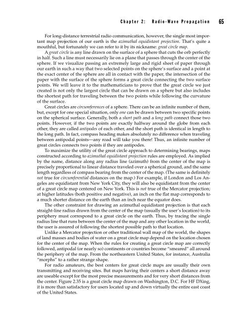
C h a p t e r 2 : r a d i o - W a v e P r o p a g a t i o n 65
For long-distance terrestrial radio communication, however, the single most important
map projection of our earth is the azimuthal equidistant projection. That’s quite a
mouthful, but fortunately we can refer to it by its nickname: great circle map.
A great circle is any line drawn on the surface of a sphere that cuts the orb perfectly
in half. Such a line must necessarily lie on a plane that passes through the center of the
sphere. If we visualize passing an extremely large and rigid sheet of paper through
our earth in such a way that two selected points on the sphere’s surface and a point at
the exact center of the sphere are all in contact with the paper, the intersection of the
paper with the surface of the sphere forms a great circle connecting the two surface
points. We will leave it to the mathematicians to prove that the great circle we just
created is not only the largest circle that can be drawn on a sphere but also includes
the shortest path for traveling between the two points while following the curvature
of the surface.
Great circles are circumferences of a sphere. There can be an infinite number of them,
but, except for one special situation, only one can be drawn between two specific points
on the spherical surface. Generally, both a short path and a long path connect those two
points. However, if the two points are exactly halfway around the globe from each
other, they are called antipodes of each other, and the short path is identical in length to
the long path. In fact, compass heading makes absolutely no difference when traveling
between antipodal points—any road will take you there! Thus, an infinite number of
great circles connects two points if they are antipodes.
To maximize the utility of the great circle approach to determining bearings, maps
constructed according to azimuthal equidistant projection rules are employed. As implied
by the name, distance along any radius line (azimuth) from the center of the map is
precisely proportional to linear distance traveled over a spherical ground, and the same
length regardless of compass bearing from the center of the map. (The same is definitely
not true for circumferential distances on the map.) For example, if London and Los Angeles
are equidistant from New York City, they will also be equidistant from the center
of a great circle map centered on New York. This is not true of the Mercator projection;
at higher latitudes (both positive and negative), an inch on the flat map corresponds to
a much shorter distance on the earth than an inch near the equator does.
The other constraint for drawing an azimuthal equidistant projection is that each
straight-line radius drawn from the center of the map (usually the user’s location) to its
periphery must correspond to a great circle on the earth. Thus, by tracing the single
radius line that runs between the center of the map and any other location in the world,
the user is assured of following the shortest possible path to that location.
Unlike a Mercator projection or other traditional wall map of the world, the shapes
of land masses and bodies of water on a great circle map depend on the location chosen
for the center of the map. When the rules for creating a great circle map are correctly
followed, antipodal (or nearly so) continents or countries become “smeared” all around
the periphery of the map. From the northeastern United States, for instance, Australia
“morphs” to a rather strange shape.
For radio amateurs, the best centers for great circle maps are usually their own
transmitting and receiving sites. But maps having their centers a short distance away
are useable except for the most precise measurements and for very short distances from
the center. Figure 2.35 is a great circle map drawn on Washington, D.C. For HF DXing,
it is more than satisfactory for users located up and down virtually the entire east coast
of the United States.