Practical_Antenna_Handbook_0071639586

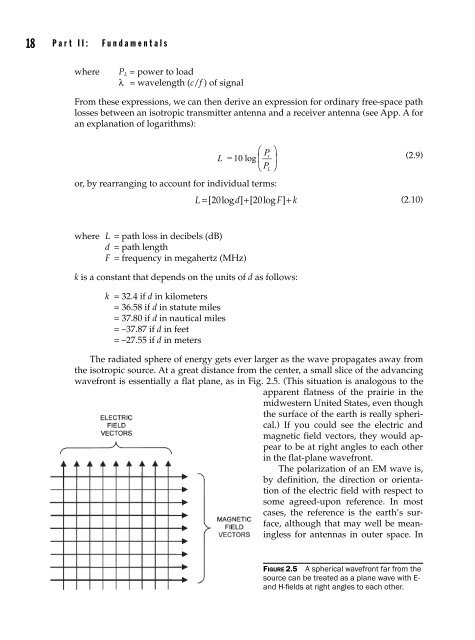
18 p a r t I I : F u n d a m e n t a l s
where
P L = power to load
l = wavelength (c/f ) of signal
From these expressions, we can then derive an expression for ordinary free-space path
losses between an isotropic transmitter antenna and a receiver antenna (see App. A for
an explanation of logarithms):
⎛ P ⎞
t
L = 10 log ⎜ ⎟
⎝ P ⎠
or, by rearranging to account for individual terms:
L = [20log d] + [20log F] + k
(2.10)
L
(2.9)
where L = path loss in decibels (dB)
d = path length
F = frequency in megahertz (MHz)
k is a constant that depends on the units of d as follows:
k = 32.4 if d in kilometers
= 36.58 if d in statute miles
= 37.80 if d in nautical miles
= –37.87 if d in feet
= –27.55 if d in meters
The radiated sphere of energy gets ever larger as the wave propagates away from
the isotropic source. At a great distance from the center, a small slice of the advancing
wavefront is essentially a flat plane, as in Fig. 2.5. (This situation is analogous to the
apparent flatness of the prairie in the
midwestern United States, even though
the surface of the earth is really spherical.)
If you could see the electric and
magnetic field vectors, they would appear
to be at right angles to each other
in the flat-plane wavefront.
The polarization of an EM wave is,
by definition, the direction or orientation
of the electric field with respect to
some agreed-upon reference. In most
cases, the reference is the earth’s surface,
although that may well be meaningless
for antennas in outer space. In
Figure 2.5 A spherical wavefront far from the
source can be treated as a plane wave with E-
and H-fields at right angles to each other.