Practical_Antenna_Handbook_0071639586

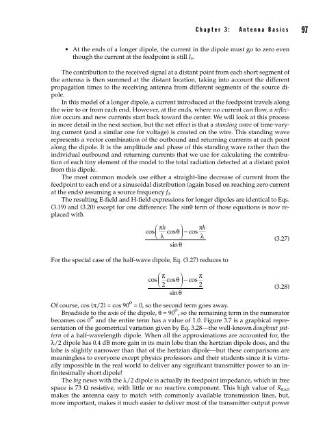
C h a p t e r 3 : A n t e n n a B a s i c s 97
• At the ends of a longer dipole, the current in the dipole must go to zero even
though the current at the feedpoint is still I 0 .
The contribution to the received signal at a distant point from each short segment of
the antenna is then summed at the distant location, taking into account the different
propagation times to the receiving antenna from different segments of the source dipole.
In this model of a longer dipole, a current introduced at the feedpoint travels along
the wire to or from each end. However, at the ends, where no current can flow, a reflection
occurs and new currents start back toward the center. We will look at this process
in more detail in the next section, but the net effect is that a standing wave of time-varying
current (and a similar one for voltage) is created on the wire. This standing wave
represents a vector combination of the outbound and returning currents at each point
along the dipole. It is the amplitude and phase of this standing wave rather than the
individual outbound and returning currents that we use for calculating the contribution
of each tiny element of the model to the total radiation detected at a distant point
from this dipole.
The most common models use either a straight-line decrease of current from the
feedpoint to each end or a sinusoidal distribution (again based on reaching zero current
at the ends) assuming a source frequency f 0 .
The resulting E-field and H-field expressions for longer dipoles are identical to Eqs.
(3.19) and (3.20) except for one difference: The sinq term of those equations is now replaced
with
⎛ πh
⎞ πh
cos cosθ
cos
⎝
⎜
λ ⎠
⎟ −
λ
sin θ
(3.27)
For the special case of the half-wave dipole, Eq. (3.27) reduces to
⎛ π ⎞ π
cos cosθ
cos
⎝
⎜ 2 ⎠
⎟ − 2
sin θ
(3.28)
Of course, cos (π/2) = cos 90 o = 0, so the second term goes away.
Broadside to the axis of the dipole, q = 90o , so the remaining term in the numerator
becomes cos 0 o and the entire term has a value of 1.0. Figure 3.7 is a graphical representation
of the geometrical variation given by Eq. 3.28—the well-known doughnut pattern
of a half-wavelength dipole. When all the approximations are accounted for, the
l/2 dipole has 0.4 dB more gain in its main lobe than the hertzian dipole does, and the
lobe is slightly narrower than that of the hertzian dipole—but these comparisons are
meaningless to everyone except physics professors and their students since it is virtually
impossible in the real world to deliver any significant transmitter power to an infinitesimally
short dipole!
The big news with the l/2 dipole is actually its feedpoint impedance, which in free
space is 73 W resistive, with little or no reactive component. This high value of R RAD
makes the antenna easy to match with commonly available transmission lines, but,
more important, makes it much easier to deliver most of the transmitter output power