Practical_Antenna_Handbook_0071639586
C h a p t e r 3 : A n t e n n a B a s i c s 91 tions, the possibility of electromagnetic waves—presumably traveling through his mystical æther—as well as the speed at which these waves must travel through space. Maxwell then went a step further: Based on the most accurate measurements of the speed of light at the time, he concluded that visible light was itself comprised of electromagnetic waves! Nearly a quarter century passed before the German scientist Heinrich Hertz demonstrated in 1887 that he could create, transmit, and receive what we now call radio waves. Hertz thus took the first baby steps in determining the physical geometry of conductors (antennas, in other words) that would allow the generation and detection of the EM radiation predicted by Maxwell. Of course, Hertz did not have any of the conveniences or inventions of the modern world; in particular, he did not have a tunable receiver or transmitter. Instead, he generated a spark (which contains a nearly infinite number of frequencies) across a gap between two curved conductors of a certain length with some laboratory equipment and attempted to detect the fields from that spark with a similar set of conductors a few feet away. The signal from his detector was then used to make a laboratory meter wiggle. And so it was that Heinrich Hertz was quite likely the first to experience the magic of radio! V BAT I(t) V(t) V = V(t) = V (1- e R s C ) CAP BAT I CHG R s = I(t) = V BAT R s e - t - t R s C Area A V(t) V BAT Conducting plates I(t) V BAT /R s R = the sum of all resistances in the circuit, including s the resistance of the interconnecting wire and the internal resistance of the battery itself. C = A d d t t Linked Electric and Magnetic Fields Now let’s return to the example of charging a capacitor from a battery. The flow of these charges constitutes a conduction current in the connecting wires that lasts for a very short time—only until the voltage across the plates of the capacitor is equal to that of the battery itself. That interval depends, of course, on the amplitude of the current, which initially is limited only by the combined resistance of the wires plus the internal resistance of the battery itself. (That’s why the wire in automobile jumper cables is so fat!) The final value of the current is zero, just as the final voltage across the capacitor is the full battery voltage, V BAT . As shown in Fig. 3.4, both voltage and current follow exponential curves during the transition period. If R s is very small, the voltage and current at the capacitor are in quadrature relationship to each other; we say they are 90 degrees out of phase, and that Figure 3.4 Exponential voltage and current when charging a capacitor.
92 P a r t I I : F u n d a m e n t a l s A B C E E E Figure 3.5 Electric field between conducting plates at various angles. the current “leads” the voltage by that amount. Specifically, I=CDV/Dt. In calculus, we would say the current flowing to the upper capacitor plate is the first derivative of the voltage across the capacitor. (Similarly, in an inductor the current “lags” the voltage by 90 degrees.) Of course, once the capacitor plates are charged, a steady E-field exists between them. Since it is a static field, it does not create a magnetic field. However, during the very short instant when current is flowing in the wires connected to the capacitor, its amplitude is constantly changing as well, which means electrons are being accelerated or decelerated and a changing magnetic field encircles each of the wires. On each wire we have both a changing current and a changing voltage within the same region of space and thus the potential for radiation, depending on the length of the wires, the space between them, and other factors. (Have you ever turned on a lamp or appliance in your home and heard a “click” in an AM broadcast receiver? That’s an example of radiation caused by the sudden change in current and voltage on the wire that runs between the switch and the appliance.) Other geometries and orientations are possible for the two capacitor plates, and they will result in different E-field patterns in the space between the plates, as shown in Fig. 3.5. If the two plates of the capacitor are spread farther apart at one end than at the other, the electric field between them must curve to always meet the plates at right angles (Fig. 3.5B and C). The straight lines in A become arcs in B, and approximately semicircles in C, where the plates are in a straight line, 180 degrees apart. But in addition to altering the orientation of the two plates with respect to each other, we can also change their shape. For instance, instead of the flat rectangular metal sheets we started with, we can make the two elements from cylindrical metal rods or wires. The Hertzian Dipole Now suppose the circle marked E in Fig. 3.6 is a transmitter or other source supplying sinusoidal RF energy at a single frequency whose wavelength is much larger than the length of the rods or wires in B. Electrons are simultaneously pushed onto one rod or wire and pulled from the other in direct response to the sinusoidal source voltage applied to the two rods. Of course, the amplitudes of the static and quasi-static E- and H-fields in the vicinity of the two rods are changing at the same sinusoidal rate as the applied voltage, but it turns out these fields exist only near the wires or rods and die out rapidly with increasing distance from the antenna. Since the velocities of the electrons are constantly changing as they shuttle back and forth between the rods and the sinusoidal source, they are in a state of continuous acceleration and deceleration, thus setting up linked time-varying electric and magnetic fields in the space enclosing the rods. Above and beyond the conventional static and quasi-static fields, Maxwell’s equations predict the existence of new fields resulting solely from the acceleration of electric charge in the region between the two rods. Spe-
- Page 58 and 59: C h a p t e r 2 : r a d i o - W a v
- Page 60 and 61: C h a p t e r 2 : r a d i o - W a v
- Page 62 and 63: C h a p t e r 2 : r a d i o - W a v
- Page 64 and 65: C h a p t e r 2 : r a d i o - W a v
- Page 66 and 67: C h a p t e r 2 : r a d i o - W a v
- Page 68 and 69: Figure 2.29C Monthly averaged sunsp
- Page 70 and 71: C h a p t e r 2 : r a d i o - W a v
- Page 72 and 73: C h a p t e r 2 : r a d i o - W a v
- Page 74 and 75: C h a p t e r 2 : r a d i o - W a v
- Page 76 and 77: C h a p t e r 2 : r a d i o - W a v
- Page 78 and 79: C h a p t e r 2 : r a d i o - W a v
- Page 80 and 81: C h a p t e r 2 : r a d i o - W a v
- Page 82 and 83: C h a p t e r 2 : r a d i o - W a v
- Page 84 and 85: C h a p t e r 2 : r a d i o - W a v
- Page 86 and 87: C h a p t e r 2 : r a d i o - W a v
- Page 88 and 89: C h a p t e r 2 : r a d i o - W a v
- Page 90 and 91: C h a p t e r 2 : r a d i o - W a v
- Page 92 and 93: C h a p t e r 2 : r a d i o - W a v
- Page 94 and 95: C h a p t e r 2 : r a d i o - W a v
- Page 96 and 97: C h a p t e r 2 : r a d i o - W a v
- Page 98 and 99: CHAPTER 3 Antenna Basics An antenna
- Page 100 and 101: C h a p t e r 3 : A n t e n n a B a
- Page 102 and 103: C h a p t e r 3 : A n t e n n a B a
- Page 104 and 105: C h a p t e r 3 : A n t e n n a B a
- Page 106 and 107: C h a p t e r 3 : A n t e n n a B a
- Page 110 and 111: C h a p t e r 3 : A n t e n n a B a
- Page 112 and 113: C h a p t e r 3 : A n t e n n a B a
- Page 114 and 115: C h a p t e r 3 : A n t e n n a B a
- Page 116 and 117: C h a p t e r 3 : A n t e n n a B a
- Page 118 and 119: C h a p t e r 3 : A n t e n n a B a
- Page 120 and 121: C h a p t e r 3 : A n t e n n a B a
- Page 122 and 123: C h a p t e r 3 : A n t e n n a B a
- Page 124 and 125: C h a p t e r 3 : A n t e n n a B a
- Page 126 and 127: CHAPTER 4 Transmission Lines and Im
- Page 128 and 129: C h a p t e r 4 : T r a n s m i s s
- Page 130 and 131: C h a p t e r 4 : T r a n s m i s s
- Page 132 and 133: C h a p t e r 4 : T r a n s m i s s
- Page 134 and 135: C h a p t e r 4 : T r a n s m i s s
- Page 136 and 137: C h a p t e r 4 : T r a n s m i s s
- Page 138 and 139: C h a p t e r 4 : T r a n s m i s s
- Page 140 and 141: C h a p t e r 4 : T r a n s m i s s
- Page 142 and 143: C h a p t e r 4 : T r a n s m i s s
- Page 144 and 145: C h a p t e r 4 : T r a n s m i s s
- Page 146 and 147: C h a p t e r 4 : T r a n s m i s s
- Page 148 and 149: C h a p t e r 4 : T r a n s m i s s
- Page 150 and 151: C h a p t e r 4 : T r a n s m i s s
- Page 152 and 153: C h a p t e r 4 : T r a n s m i s s
- Page 154 and 155: C h a p t e r 4 : T r a n s m i s s
- Page 156 and 157: C h a p t e r 4 : T r a n s m i s s
C h a p t e r 3 : A n t e n n a B a s i c s 91<br />
tions, the possibility of electromagnetic waves—presumably traveling through his mystical<br />
æther—as well as the speed at which these waves must travel through space.<br />
Maxwell then went a step further: Based on the most accurate measurements of the<br />
speed of light at the time, he concluded that visible light was itself comprised of electromagnetic<br />
waves!<br />
Nearly a quarter century passed before the German scientist Heinrich Hertz demonstrated<br />
in 1887 that he could create, transmit, and receive what we now call radio<br />
waves. Hertz thus took the first baby steps in determining the physical geometry of<br />
conductors (antennas, in other words) that would allow the generation and detection of<br />
the EM radiation predicted by Maxwell. Of course, Hertz did not have any of the conveniences<br />
or inventions of the modern world; in particular, he did not have a tunable<br />
receiver or transmitter. Instead, he generated a spark (which contains a nearly infinite<br />
number of frequencies) across a gap between two curved conductors of a certain length<br />
with some laboratory equipment and attempted to detect the fields from that spark<br />
with a similar set of conductors a few feet away. The signal from his detector was then<br />
used to make a laboratory meter wiggle. And so it was that Heinrich Hertz was quite<br />
likely the first to experience the magic of radio!<br />
V BAT<br />
I(t)<br />
V(t)<br />
V = V(t) = V (1- e R s<br />
C )<br />
CAP BAT<br />
I<br />
CHG<br />
R s<br />
= I(t) = V<br />
BAT<br />
R s<br />
e<br />
- t<br />
- t<br />
R s<br />
C<br />
Area A<br />
V(t)<br />
V BAT<br />
Conducting plates<br />
I(t)<br />
V BAT /R s<br />
R = the sum of all resistances in the circuit, including<br />
s<br />
the resistance of the interconnecting wire and<br />
the internal resistance of the battery itself.<br />
C = A<br />
d<br />
d<br />
t<br />
t<br />
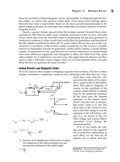
Linked Electric and Magnetic Fields<br />
Now let’s return to the example of charging a capacitor from a battery. The flow of these<br />
charges constitutes a conduction current in the connecting wires that lasts for a very<br />
short time—only until the voltage<br />
across the plates of the capacitor<br />
is equal to that of the battery<br />
itself. That interval depends, of<br />
course, on the amplitude of the<br />
current, which initially is limited<br />
only by the combined resistance<br />
of the wires plus the internal<br />
resistance of the battery itself.<br />
(That’s why the wire in automobile<br />
jumper cables is so fat!) The<br />
final value of the current is zero,<br />
just as the final voltage across the<br />
capacitor is the full battery voltage,<br />
V BAT . As shown in Fig. 3.4,<br />
both voltage and current follow<br />
exponential curves during the<br />
transition period.<br />
If R s is very small, the voltage<br />
and current at the capacitor<br />
are in quadrature relationship to<br />
each other; we say they are 90<br />
degrees out of phase, and that<br />
Figure 3.4 Exponential voltage and<br />
current when charging a capacitor.


