Ecuatii Diferentiale
Ecuatii Diferentiale
Ecuatii Diferentiale

Create successful ePaper yourself
Turn your PDF publications into a flip-book with our unique Google optimized e-Paper software.
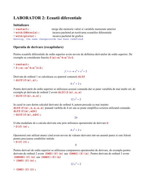
LABORATOR 2: <strong>Ecuatii</strong> diferentiale<br />
Initializare<br />
> restart: sterge din memorie valori si variabile memorate anterior<br />
> with(DEtools): incarca pachetul pt rezolvarea ecuatiilor diferentiale<br />
> with(plots): incarca pachetul de grafica<br />
Warning, the name changecoords has been redefined<br />
Operatia de derivare (recapitulare)<br />
Pentru ecuatiile diferentiale de ordin superior avem nevoie de definirea derivatelor de ordin superior. De<br />
exemplu sa consideram functia f(x)=x^4+x^2+2.<br />
> restart:<br />
> f:=x->x^4+x^2+2;<br />
f := x → + +<br />
Derivata de ordinul 1 se calculeaza cu ajutorul comenzii diff<br />
> diff(f(x),x);<br />
4 x +<br />
3<br />
2 x<br />
Pentru derivatele de ordin superior se utilizeaza aceeasi comanda dar se pune variabila de mai multe ori, de<br />
exemplu pt derivata de ordinul 2 avem diff(f(x),x,x)<br />
> diff(f(x),x,x);<br />
12 x +<br />
2<br />
2<br />
In cazul in care dorim calculul derivatei de ordinul 4, putem proceda ca mai inainte:<br />
diff(f(x),x,x,x,x) punand varibila de 4 ori sau se poate simplifica scrierea utilizand comanda:<br />
diff(f(x),x$4)<br />
> diff(f(x),x$4);<br />
24<br />
O alta modaliate de a calcula derivata este prin utilizarea operatorului de derivare D<br />
> D(f)(x);<br />
4 x +<br />
3<br />
2 x<br />
Operatorul este utilizat atunci cind avem nevoie de valoare derivatei intr-un anumit punct si este folosit<br />
pentru precizarea conditiilor initiale<br />
> D(f)(0);<br />
0<br />
Pentru derivari de ordin superior se utilizeaza compunerea operatorului de derivare, de exemplu pentru<br />
derivata de ordinul 2 avem (D@D)(f)(x) sau (D@@2)(f)(x). Pentru derivata de ordinul 3 avem<br />
(D@D@D)(f)(x) sau (D@@3)(f)(x)<br />
> (D@D)(f)(x);<br />
12 x +<br />
2<br />
2<br />
> (D@D)(f)(2);<br />
x 4<br />
x 2<br />
2
(D@@2)(f)(x);<br />
> (D@@4)(f)(x);<br />
50<br />
12 x +<br />
2<br />
2<br />
Definirea si rezolvarea unei ecuatii diferentiale<br />
Fie ecuatia diferentiala de ordinul 1: y'(x)=sin(x)*(y(x))^2. Aceasta ecuatie este o ecuatie cu<br />
variabile separabile adica este forma y'(x)=f(x)*g(y). Ecuatia se defineste in MAPLE utilizand<br />
comanda diff dupa cum urmeaza:<br />
> ecdif1:=diff(y(x),x) =sin(x)*(y(x))^2;<br />
d<br />
2<br />
ecdif1 := y( x ) = sin( x ) y( x )<br />
dx<br />
24<br />
Pentru a obtine solutia generala se utilizeaza comanda dsolve(ecuatie, functie necunoscuta)<br />
> dsolve(ecdif1,y(x));<br />
1<br />
y( x ) =<br />
cos( x ) + _C1<br />
Metodele incercate si utilizate de MAPLE pentru a obtine solutiile ecuatiilor diferentiale pot fi observate<br />
crescand infolevel pentru dsolve la 3:<br />
> infolevel[dsolve]:=3;<br />
:= 3<br />
apoi reexecutam comanda dsolve:<br />
> dsolve(ecdif1,y(x));<br />
Methods for first order ODEs:<br />
--- Trying classification methods ---<br />
trying a quadrature<br />
trying 1st order linear<br />
trying Bernoulli<br />
Pentru a vedea care sunt metodele de rezolvare a ecuatiilor de ordinul 1 implementate in dsolve se poate da<br />
comanda:<br />
> `dsolve/methods`[1];<br />
[ quadrature, linear, Bernoulli, separable, inverse_linear, homogeneous, Chini, lin_sym,<br />
exact, Abel, pot_sym]<br />
Pentru alte amanunte legate de comanda dsolve executati:<br />
> ?dsolve;<br />
Pentru suprimarea informatiilor suplimentare resetam infolevel pentru dsolve la 0<br />
> infolevel[dsolve]:=0;<br />
:= 0<br />
infolevel dsolve<br />
In unele cazuri este mai convenabil obtinerea solutiilor in forma implicita, acest lucru se poate realiza<br />
specificand in cadrul procedurii dsolve optiunea implicit. De exemplu, sa consideram ecuatia<br />
diferentiala (3y^2 + e^x) y'+e^x (y + 1) + cos x = 0:<br />
> ecdif2:=(3*y(x)^2+exp(x))*diff(y(x),x)+exp(x)*(y(x)+1)+cos(x) = 0;<br />
ecdif2 := ( 3 y( x ) + ) + + =<br />
2 x<br />
e<br />
⎛ d ⎞<br />
⎝<br />
⎜ ( )<br />
dx<br />
⎠<br />
⎟ y x e x ( y( x ) + 1 ) cos( x ) 0<br />
> dsolve(ecdif2,y(x),implicit);<br />
e + + + + =<br />
x<br />
y( x ) e x<br />
sin( x ) y( x )<br />
3<br />
_C1 0<br />
Pentru a vedea avantajul, incercati sa rezolvati ecuatia fara a preciza optiunea implicit.<br />
Pentru ecuatiile diferentiale de ordinul 2 se foloseste aceeasi metoda, se defineste ecuatia si apoi se utilizeaza<br />
comanda dsolve. De exemplu sa consideram ecuatia y''(x)+3y'(x)+2y(x)=1+x^2<br />
> ecdif3:=diff(y(x),x$2)+3*diff(y(x),x)+2*y(x)=1+x^2;<br />
⎛ d<br />
ecdif3 := ⎜<br />
⎞<br />
⎟ + + =<br />
⎝<br />
⎜d<br />
⎠<br />
⎟<br />
2<br />
x 2 y( x ) 3 ⎛ d ⎞<br />
⎝<br />
⎜ y( x )<br />
dx<br />
⎠<br />
⎟ 2 y( x ) 1 + x2<br />
> dsolve(ecdif3,y(x));<br />
x<br />
y( x ) = − + − +<br />
2<br />
3 x 9 ( −2 x )<br />
e _C1 e<br />
2 2 4<br />
Reprezentarea grafica a solutiilor<br />
> with(plots):<br />
Warning, the name changecoords has been redefined<br />
Sa consideram, din nou, prima ecuatie: y'(x)=sin(x)*(y(x))^2.<br />
> ecdif1:=diff(y(x),x) =sin(x)*(y(x))^2;<br />
d<br />
2<br />
ecdif1 := y( x ) = sin( x ) y( x )<br />
dx<br />
> sol1:=dsolve(ecdif1,y(x));<br />
1<br />
sol1 := y( x ) =<br />
cos( x ) + _C1<br />
( ) −x<br />
_C2
Rezultatul comenzii dsolve nu este o functie, ci este o ecuatie. Pentru manipularea solutiei exista doua<br />
alternative, fie definim functia ce reprezinta solutia (in situatia in care expresia ei nu e prea complicata), in<br />
cazul dat solutia depinde de variabila independenta x si constanta de integrare:<br />
> y1:=(x,c)->1/(cos(x)+c);<br />
1<br />
y1 := ( xc , ) →<br />
cos( x) + c<br />
sau avem acces la membrul drept utilizand comanda rhs (right hand side) si apoi comanda unapply<br />
pentru a construi solutia ca functie<br />
> right_hand_expr:=rhs(sol1);<br />
right_hand_expr :=<br />
1<br />
cos( x ) + _C1<br />
Prin comanda unapply se transforma expresia right_hand_expr in functie precizand variabilele<br />
acesteia:<br />
> y2:=unapply(right_hand_expr,x,_C1);<br />
1<br />
y2 := ( x, _C1 ) →<br />
cos( x ) + _C1<br />
Pentru reprezentarea grafica a catorva solutii dam valori constantei c, de exemplu c:=2, c:=3 si c:=4<br />
> plot([y1(x,2),y1(x,3),y1(x,4)],x=-2*Pi..2*Pi);<br />
Daca se doreste obtinerea graficelor cu anumite culori precizate vom utiliza urmatoarea comanda:<br />
> plot([y1(x,2),y1(x,3),y1(x,4)],x=-2*Pi..2*Pi,color=[black,red,blue]);
In cazul celei de a doua ecuatii, (3y^2 + e^x) y'+e^x (y + 1) + cos x = 0, unde solutia este<br />
obtinuta in forma implicita, trebuie utilizata procedura implicitplot.<br />
> ecdif2:=(3*y(x)^2+exp(x))*diff(y(x),x)+exp(x)*(y(x)+1)+cos(x) = 0;<br />
ecdif2 := ( 3 y( x ) + ) + + =<br />
2 x<br />
e<br />
⎛ d ⎞<br />
⎝<br />
⎜ ( )<br />
dx<br />
⎠<br />
⎟ y x e x ( y( x ) + 1 ) cos( x ) 0<br />
> sol2:=dsolve(ecdif2,y(x),implicit);<br />
sol2 := e + + + + =<br />
x<br />
y( x ) e x<br />
sin( x ) y( x )<br />
3<br />
_C1 0<br />
Construim functia care ne da ecuatia implicita a solutiilor, in acest caz, expresia se afla in partea stanga a<br />
ecuatiei si vom folosi comanda lhs (letf hand side) pentru a avea acces la aceasta expresie<br />
> left_hand_side:=lhs(sol2);<br />
left_hand_side := e + + + +<br />
x<br />
y( x ) e x<br />
sin( x ) y( x )<br />
3<br />
_C1<br />
> lhs1:=subs( y(x)=y, left_hand_side );<br />
lhs1 := e + + + +<br />
x y e x<br />
sin( x) y 3<br />
_C1<br />
> f:=unapply(lhs1,x,y,_C1);<br />
f := ( x, y, _C1 ) → e + + + +<br />
x y e x<br />
sin( x) y 3<br />
_C1<br />
> implicitplot({f(x,y,0)=0,f(x,y,0.5)=0,f(x,y,1)=0},x=-5..5,y=-<br />
5..5,numpoints=10000);<br />
Daca dorim reprezentarea grafica a mai multor solutii, putem genera un sir de functii f(x,y,c) pentru<br />
c =-4, -19/5, ...,-1/5, 0, 1/5, 2/5, ..., 4 folosim comanda seq dupa cum urmeaza<br />
> sir_sol:=seq(f(x,y,i/5)=0,i=-20..20);<br />
sir_sol e + + + − =<br />
x y e x<br />
sin( x) y 3<br />
4 0 e + + + − =<br />
x y e x<br />
sin( x) y 3 19<br />
:=<br />
, 0,<br />
5<br />
e + + + − =<br />
x y e x<br />
sin( x) y 3 18<br />
0 e + + + − =<br />
5<br />
x y e x<br />
sin( x) y 3 17<br />
, 0,<br />
5<br />
e + + + − =<br />
x y e x<br />
sin( x) y 3 16<br />
0 e + + + − =<br />
5<br />
x y e x<br />
sin( x) y 3<br />
, 3 0,<br />
e + + + − =<br />
x y e x<br />
sin( x) y 3 14<br />
0 e + + + − =<br />
5<br />
x y e x<br />
sin( x) y 3 13<br />
, 0,<br />
5
e + + + − =<br />
x y e x<br />
sin( x) y 3 12<br />
0 e + + + − =<br />
5<br />
x y e x<br />
sin( x) y 3 11<br />
, 0,<br />
5<br />
e + + + − =<br />
x y e x<br />
sin( x) y 3<br />
2 0 e + + + − =<br />
x y e x<br />
sin( x) y 3 9<br />
, 0,<br />
5<br />
e + + + − =<br />
x y e x<br />
sin( x) y 3 8<br />
0 e + + + − =<br />
5<br />
x y e x<br />
sin( x) y 3 7<br />
, 0,<br />
5<br />
e + + + − =<br />
x y e x<br />
sin( x) y 3 6<br />
0 e + + + − =<br />
5<br />
x y e x<br />
sin( x) y 3<br />
, 1 0,<br />
e + + + − =<br />
x y e x<br />
sin( x) y 3 4<br />
0 e + + + − =<br />
5<br />
x y e x<br />
sin( x) y 3 3<br />
, 0,<br />
5<br />
e + + + − =<br />
x y e x<br />
sin( x) y 3 2<br />
0 e + + + − =<br />
5<br />
x y e x<br />
sin( x) y 3 1<br />
, 0,<br />
5<br />
e + + + =<br />
x y e x<br />
sin( x) y 3<br />
0 e + + + + =<br />
x y e x<br />
sin( x) y 3 1<br />
, 0,<br />
5<br />
e + + + + =<br />
x y e x<br />
sin( x) y 3 2<br />
0 e + + + + =<br />
5<br />
x y e x<br />
sin( x) y 3 3<br />
, 0,<br />
5<br />
e + + + + =<br />
x y e x<br />
sin( x) y 3 4<br />
0 e + + + + =<br />
5<br />
x y e x<br />
sin( x) y 3<br />
, 1 0,<br />
e + + + + =<br />
x y e x<br />
sin( x) y 3 6<br />
0 e + + + + =<br />
5<br />
x y e x<br />
sin( x) y 3 7<br />
, 0,<br />
5<br />
e + + + + =<br />
x y e x<br />
sin( x) y 3 8<br />
0 e + + + + =<br />
5<br />
x y e x<br />
sin( x) y 3 9<br />
, 0,<br />
5<br />
e + + + + =<br />
x y e x<br />
sin( x) y 3<br />
2 0 e + + + + =<br />
x y e x<br />
sin( x) y 3 11<br />
, 0,<br />
5<br />
e + + + + =<br />
x y e x<br />
sin( x) y 3 12<br />
0 e + + + + =<br />
5<br />
x y e x<br />
sin( x) y 3 13<br />
, 0,<br />
5<br />
e + + + + =<br />
x y e x<br />
sin( x) y 3 14<br />
0 e + + + + =<br />
5<br />
x y e x<br />
sin( x) y 3<br />
, 3 0,<br />
e + + + + =<br />
x y e x<br />
sin( x) y 3 16<br />
0 e + + + + =<br />
5<br />
x y e x<br />
sin( x) y 3 17<br />
, 0,<br />
5<br />
e + + + + =<br />
x y e x<br />
sin( x) y 3 18<br />
0 e + + + + =<br />
5<br />
x y e x<br />
sin( x) y 3 19<br />
, 0,<br />
5<br />
e + + + + =<br />
x y e x<br />
sin( x) y 3<br />
4 0<br />
> implicitplot({sir_sol},x=-5..5,y=-5..5,numpoints=10000);
In cazul ecuatiei de ordinul 2, y''(x)+3y'(x)+2y(x)=1+x^2, reprezentarea grafica a solutiilor revine<br />
la particularizarea celor doua constante de integrare<br />
> ecdif3:=diff(y(x),x$2)+3*diff(y(x),x)+2*y(x)=1+x^2;<br />
⎛ d<br />
ecdif3 := ⎜<br />
⎞<br />
⎟ + + =<br />
⎝<br />
⎜d<br />
⎠<br />
⎟<br />
2<br />
x 2 y( x ) 3 ⎛ d ⎞<br />
⎝<br />
⎜ y( x )<br />
dx<br />
⎠<br />
⎟ 2 y( x ) 1 + x2<br />
> sol3:=dsolve(ecdif3,y(x));<br />
x<br />
sol3 := y( x ) = − + − +<br />
2<br />
3 x 9 ( −2 x )<br />
e _C1 e<br />
2 2 4<br />
( ) −x<br />
> right_hand_expr:=rhs(sol3);<br />
x<br />
right_hand_expr := − + − +<br />
2<br />
3 x 9 ( −2 x )<br />
e _C1 e<br />
2 2 4<br />
_C2<br />
( ) −x<br />
_C2<br />
> y1:=unapply(right_hand_expr,x,_C1,_C2);<br />
1<br />
y1 := ( x, _C1, _C2 ) → − + − +<br />
2 x2 3<br />
2 x<br />
9 ( −2 x )<br />
( )<br />
e _C1 e<br />
4<br />
−x<br />
_C2<br />
> plot([y1(x,0,0),y1(x,-1,1),y1(x,1,-1)],x=-1..2,color=[black,blue,red]);<br />
sau putem repezenta un sir de solutii:<br />
> sir_sol3:=seq(seq(y1(x,i/5,j/2),i=-2..2),j=-2..2);<br />
x<br />
sir_sol3 − + + −<br />
2<br />
3 x 9 2 ( −2 x ) ( )<br />
e e<br />
2 2 4 5 −x x<br />
− + + −<br />
2<br />
3 x 9 1 ( −2 x ) ( )<br />
e e<br />
2 2 4 5 −x<br />
:=<br />
, ,<br />
x<br />
− + −<br />
2<br />
3 x 9 ( )<br />
e<br />
2 2 4<br />
−x x<br />
− + − −<br />
2<br />
3 x 9 1 ( −2 x ) ( )<br />
e e<br />
2 2 4 5 −x x<br />
− + − −<br />
2<br />
3 x 9 2 ( −2 x ) ( )<br />
e e<br />
2 2 4 5 −x<br />
, , ,<br />
x<br />
− + + −<br />
2<br />
3 x 9 2 ( −2 x ) 1 ( )<br />
e e<br />
2 2 4 5 2 −x x<br />
− + + −<br />
2<br />
3 x 9 1 ( −2 x ) 1 ( )<br />
e e<br />
2 2 4 5 2 −x<br />
, ,<br />
x<br />
− + −<br />
2<br />
3 x 9 1 ( )<br />
e<br />
2 2 4 2 −x x<br />
− + − −<br />
2<br />
3 x 9 1 ( −2 x ) 1 ( )<br />
e e<br />
2 2 4 5 2 −x<br />
, ,<br />
x<br />
− + − −<br />
2<br />
3 x 9 2 ( −2 x ) 1 ( )<br />
e e<br />
2 2 4 5 2 −x x<br />
− + +<br />
2<br />
3 x 9 2 ( −2 x ) x<br />
e − + +<br />
2 2 4 5 2<br />
3 x 9 1 ( −2 x )<br />
, , e ,<br />
2 2 4 5<br />
1<br />
− +<br />
2 x2 3<br />
2 x<br />
9 x<br />
− + −<br />
4<br />
2<br />
3 x 9 1 ( −2 x ) x<br />
e − + −<br />
2 2 4 5 2<br />
3 x 9 2 ( −2 x )<br />
, , e ,<br />
2 2 4 5
x<br />
− + + +<br />
2<br />
3 x 9 2 ( −2 x ) 1 ( )<br />
e e<br />
2 2 4 5 2 −x x<br />
− + + +<br />
2<br />
3 x 9 1 ( −2 x ) 1 ( )<br />
e e<br />
2 2 4 5 2 −x<br />
, ,<br />
x<br />
− + +<br />
2<br />
3 x 9 1 ( )<br />
e<br />
2 2 4 2 −x x<br />
− + − +<br />
2<br />
3 x 9 1 ( −2 x ) 1 ( )<br />
e e<br />
2 2 4 5 2 −x<br />
, ,<br />
x<br />
− + − +<br />
2<br />
3 x 9 2 ( −2 x ) 1 ( )<br />
e e<br />
2 2 4 5 2 −x x<br />
− + + +<br />
2<br />
3 x 9 2 ( −2 x ) ( )<br />
e e<br />
2 2 4 5 −x<br />
, ,<br />
x<br />
− + + +<br />
2<br />
3 x 9 1 ( −2 x ) ( )<br />
e e<br />
2 2 4 5 −x x<br />
− + +<br />
2<br />
3 x 9 ( )<br />
e<br />
2 2 4<br />
−x x<br />
− + − +<br />
2<br />
3 x 9 1 ( −2 x )<br />
, ,<br />
e e<br />
2 2 4 5<br />
x<br />
− + − +<br />
2<br />
3 x 9 2 ( −2 x ) ( )<br />
e e<br />
2 2 4 5 −x<br />
> plot([sir_sol3],x=-1..1);<br />
Rezolvarea problemelor cu valori initiale (Probleme Cauchy)<br />
In general, rezolvarea anumitor probleme revin la determinarea unei solutii pentru o ecuatie diferentiala ce<br />
satisface anumite conditii initiale. Aceste probleme se numesc probleme cu valori initiale sau probleme<br />
Cauchy. De exemplu, sa presupunem ca trebuie determinata solutia ecuatiei y'(x)=sin(x)*(y(x))^2<br />
ce satisface conditia y(0)=1/3, adica solutia reprezentata in paragraful anterior pentru constanta c=2<br />
> restart:with(DEtools):<br />
> ecdif1:=diff(y(x),x) =sin(x)*(y(x))^2;<br />
d<br />
2<br />
ecdif1 := y( x ) = sin( x ) y( x )<br />
dx<br />
Definim conditia initiala:<br />
> cond_in:=y(0)=1/3;<br />
1<br />
cond_in := y0 ( ) =<br />
3<br />
Comanda de rezolvare a problemei Cauchy este similara cu cea de rezolvare a ecuatiei la care se adauga si<br />
conditia initiala:<br />
> sol1:=dsolve({ecdif1,cond_in},y(x));<br />
1<br />
sol1 := y( x ) =<br />
cos( x ) + 2<br />
Pentru reprezentarea grafica a solutiei se utilizeaza comanda rhs:<br />
> y1:=unapply(rhs(sol1),x);<br />
( ) −x<br />
,
plot(y1(x),x=-2*Pi..2*Pi);<br />
y1 := x →<br />
1<br />
cos( x ) + 2<br />
Se poate obtine graficul solutiei problemei Cauchy utilizand comanda DEplot:<br />
> DEplot(ecdif1,y(x),x=-2*Pi..2*Pi,[[cond_in]],stepsize=0.1);<br />
Se observa ca in aceasta reprezentare apare si campul de directii impreuna cu solutia. Daca se doreste<br />
reprezentarea grafica a solutiilor pentru diverse conditii initiale, de exemplu y(0)=1/3, y(0)=1/4,<br />
y(0)=1/5, se utilizeaza aceeasi comanda specificand lista de conditii initiale:<br />
> DEplot(ecdif1,y(x),x=-<br />
2*Pi..2*Pi,[[y(0)=1/3],[y(0)=1/4],[y(0)=1/5]],stepsize=0.1,linecolor=[bla<br />
ck,red,blue]);
Daca dorim reprezentarea grafica doar a campului de directii se utilizeaza comanda:<br />
> DEplot(ecdif1,y(x),x=-2*Pi..2*Pi,y=-1..1);<br />
Acelasi rezultat se obtine utilizand si comanda dfieldplot:<br />
> dfieldplot(ecdif1,y(x),x=-2*Pi..2*Pi,y=-1..1);<br />
In cazul ecuatiilor diferentiale de ordinul 2 problema Cauchy va avea doua conditii initiale y(x0)=a si<br />
y'(x0)=b. Definirea celei de a doua conditii se face cu ajutorul operatorului de derivare D. De exemplu, sa<br />
determinam solutia ecuatiei y''(x)+3y'(x)+2y(x)=1+x^2 ce satisface conditiile initiale y(0)=0 si<br />
y'(0)=1<br />
> ecdif3:=diff(y(x),x$2)+3*diff(y(x),x)+2*y(x)=1+x^2;<br />
⎛ d<br />
ecdif3 := ⎜<br />
⎞<br />
⎟ + + =<br />
⎝<br />
⎜d<br />
⎠<br />
⎟<br />
2<br />
x 2 y( x ) 3 ⎛ d ⎞<br />
⎝<br />
⎜ y( x )<br />
dx<br />
⎠<br />
⎟ 2 y( x ) 1 + x2<br />
> cond_in:=y(0)=0,D(y)(0)=1;<br />
cond_in := y0 ( ) = 0 , D( y ) ( 0) = 1<br />
> sol3:=dsolve({ecdif3,cond_in},y(x));<br />
x<br />
sol3 := y( x ) = − + − −<br />
2<br />
3 x 9 1 ( −2 x )<br />
e<br />
2 2 4 4<br />
( )<br />
2 e −x<br />
Pentru reprezentarea grafica a solutiei fie utilizam metoda de constructie a solutiei cu rhs si unapply sau,<br />
direct, prin DEplot<br />
> rhs3:=rhs(sol3);
y3:=unapply(rhs3,x);<br />
> plot(y3(x),x=-2..5);<br />
3 x 9 1 ( −2 x )<br />
rhs3 := − + − e −<br />
2 2 4 4<br />
x 2<br />
1<br />
y3 := x → − + − −<br />
2 x2 3<br />
2 x<br />
9 1 ( −2 x )<br />
e<br />
4 4<br />
( )<br />
2 e −x<br />
( )<br />
2 e −x<br />
> DEplot(ecdif3,y(x),x=-2..5,[[cond_in]],stepsize=0.1);