Curso de Equações Diferenciais Ordinárias - Unesp
Curso de Equações Diferenciais Ordinárias - Unesp
Curso de Equações Diferenciais Ordinárias - Unesp

You also want an ePaper? Increase the reach of your titles
YUMPU automatically turns print PDFs into web optimized ePapers that Google loves.
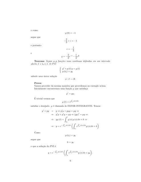
e como<br />
segue que<br />
y (0) = −1<br />
− 2 3 + c = −1<br />
e portanto<br />
e<br />
c = − 1 3<br />
y = − 2 3 e−t − 1 3 e t 2<br />
Teorema: Sejam p, g funções reais contínuas <strong>de</strong>finidas em um intervalo<br />
aberto I e t 0 ∈ I. O PVI<br />
{ y ′ + p (t) y = g (t)<br />
admite uma única solução<br />
y (t 0 ) = y 0<br />
φ : I → R.<br />
Prova:<br />
Vamos proce<strong>de</strong>r da mesma maneira que proce<strong>de</strong>mos no exemplo acima.<br />
Inicialmente encontremos uma função µ que satisfaça<br />
É trivial vermos que<br />
µ ′ = pµ.<br />
R t<br />
p(s)ds<br />
t<br />
µ (t) = e 0<br />
satisfaz o <strong>de</strong>sejado. µ é chamada <strong>de</strong> FATOR INTEGRANTE. Temos:<br />
Como<br />
segue que<br />
y ′ + py = g ⇒ y ′ µ + pµy = µg ⇒<br />
⇒<br />
y ′ µ + µ ′ y = µg ⇒ (yµ) ′ = µg ⇒<br />
∫ t<br />
⇒ yµ (t) = g (s) µ (s) ds + k ⇒<br />
t 0<br />
⇒ y = e − R (∫<br />
t<br />
t R<br />
)<br />
p(s)ds<br />
s<br />
t 0 t p(u)du 0 g (s) ds + k<br />
y (t 0 ) = y 0<br />
k = y 0<br />
t 0<br />
e<br />
e que a solução do PVI é<br />
y = e − R (∫<br />
t<br />
t R<br />
)<br />
p(s)ds<br />
s<br />
t 0 t<br />
e<br />
p(u)du 0 g (s) ds + y 0 .<br />
t 0<br />
6