Curso de Equações Diferenciais Ordinárias - Unesp

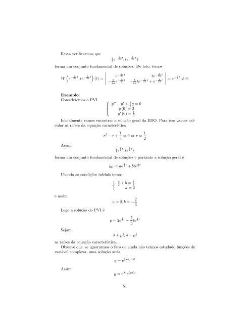
Resta verificarmos que
{e − b
2a t , te − b
2a t }
forma um conjunto fundamental de soluções. De fato, temos
∣
(
W e − b
2a t , te − b t) e
2a (t) =
− b
2a t
te − b
2a t ∣∣∣∣ ∣ − b
2a e− b
2a t − b
2a te− b
2a t + e − b
2a t = e − b a t ≠ 0.
Exemplo:
Consideremos o PVI ⎧
⎨ y ′′ − y ′ + 1 4 y = 0
y (0) = 2
⎩
y ′ (0) = 1 3
Inicialmente vamos encontrar a solução geral da EDO. Para isso vamos calcular
as raízes da equação característica
Assim
r 2 − r + 1 4 = 0 ⇔ r = 1 2
{e 1 2 t , te 1 2 t }
forma um conjunto fundamental de soluções e portanto a solução geral é
y G = ae 1 2 t + bte 1 2 t
Usando as condições iniciais temos
{ a
2 + b = 1 3
a = 2
e assim
Logo a solução do PVI é
Sejam
a = 2, b = − 2 3
y = 2e 1 2 t − 2 3 te 1 2 t
λ + µi, λ − µi
as raízes da equação característica.
Observe que, se ignorarmos o fato de ainda não termos estudado funções de
variável complexa, uma solução seria
y = e (λ+µi)t
Assim
y = e λt e (µt)i
51