Curso de Equações Diferenciais Ordinárias - Unesp

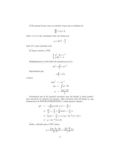
2) Da mesma forma como no anterior temos que as soluções de
dy
dt
= ry + k,
onde r ≠ 0 e k são constantes reais, são dadas por
onde M é uma constante real.
3) Vamos resolver o PVI
y = Me rt − k r
{ y ′ − y 2 = e−t
y (0) = −1
Multipliquemos os dois lados da equação por µ (t) :
µy ′ − µ y 2 = µe−t
Suponhamos que
−µ y 2 = µ′ y
e temos
(µy) ′ = µe −t
∫
µy = µe −t dt
y =
∫
µe −t dt
µ
Concluímos que se for possível encontrar uma tal função µ então poderemos
encontrar as soluções da equação. Mas encontrar uma tal função µ, que
chamaremos de FATOR INTEGRANTE, é relativamente simples:
yµ ′ = −µ y 2 (y ≠ 0) ⇒ µ′ = − µ 2 ⇒
⇒ µ′
µ = −1 2 ⇒ d dt ln |µ| = −1 2 ⇒
⇒
ln |µ| = − t 2 + c ⇒ |µ| = ke− t 2 , k > 0 ⇒
⇒ µ = ke − t 2 , k ∈ R.
Assim, voltando para o PVI, temos
y =
∫
ke
− t 2 e −t dt
ke − t 2
5
= − 2 3t
3e− 2 + c
e − t 2