My title - Departamento de Matemática da Universidade do Minho
My title - Departamento de Matemática da Universidade do Minho
My title - Departamento de Matemática da Universidade do Minho

You also want an ePaper? Increase the reach of your titles
YUMPU automatically turns print PDFs into web optimized ePapers that Google loves.
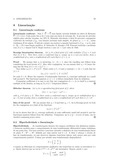
8<br />
LINEARIZAÇÃO 59<br />
8 Linearização<br />
8.1 Linearização conforme<br />
Linearização conforme. Seja f : C → C uma função racional <strong>de</strong>fini<strong>da</strong> na esfera <strong>de</strong> Riemann<br />
C = C ∪ {∞}. Ca<strong>da</strong> ponto fixo p <strong>de</strong> f tem uma sua bacia <strong>de</strong> actração B p . A procura <strong>de</strong> meto<strong>do</strong>s<br />
rápi<strong>do</strong>s para calcular itera<strong>da</strong>s, em 1871 E. Schrœ<strong>de</strong>r introduziu a i<strong>de</strong>ia <strong>de</strong> procurar conjugações<br />
conformes <strong>da</strong> restrição f ∣ Bp com funções racionais mais simples, <strong>do</strong> género g : z ↦→ λz , numa<br />
vizinhança B <strong>da</strong> origem. O méto<strong>do</strong> consiste em resolver a equação funcional h◦f ∣ Bp = g ◦h, on<strong>de</strong><br />
h : B p → B é uma função analítica. E. Schrœ<strong>de</strong>r, G. Kœnig e J.H. Poincaré trataram o problema<br />
com |λ| ≠ 1, e <strong>de</strong>pois Carl S. Siegel resolveu o caso |λ| = 1 por volta <strong>de</strong> 1940.<br />
Koenigs linearization theorem. Let z 0 be a fixed point of f with multiplier f ′ (z 0 ) = λ such<br />
that |λ| ≠ 0, 1. Then there exists a conformal map φ, unique up to a non-zero factor, from a<br />
neighborhood of z 0 onto a neighborhood of 0 such that φ ◦ f = λ · φ.<br />
Proof. We assume that z 0 is attracting, i.e. |λ| < 1, since the repelling case follows from<br />
consi<strong>de</strong>ring the local inverse of f. Also, after conjugation, we can assume that z 0 = 0, hence the<br />
map has the form f(z) = λz + a 2 z 2 + ....<br />
Now <strong>de</strong>fine φ n (z) = f n (z)/λ n . There exists a δ > 0 and a constant c < |λ| < 1 such that for<br />
|z| < δ<br />
|φ n+1 (z) − φ n (z)| ≤ k · (c/|λ|) n<br />
for some k > 0. Hence the sequence of holomorphic functions φ n converges uniformly in a small<br />
ball around 0. The functional equation φ ◦ f = λ · φ follows immediatly from its <strong>de</strong>finition.<br />
Comparing coefficients it is easy to see that any conjugation of z ↦→ λz to itself is a constant<br />
multiple of the i<strong>de</strong>ntity, as long as |λ| ≠ 0, 1. Uniqueness follows.<br />
Böttcher theorem<br />
Let z 0 be a superattracting fixed point of f, where<br />
f(z) = z 0 + a p (z − z 0 ) p + ...<br />
with a p ≠ 0 and p ≥ 2. Then there exists a conformal map φ, unique up to multiplication by a<br />
(p − 1)-root of unity, from a neighborhood of z 0 onto a neighborhood of 0 such that φ ◦ f = φ p .<br />
I<strong>de</strong>a of the proof. We can assume that z 0 = 0 and that a p = 1. As in Koenigs proof, we look<br />
for the conjugation as a limit af the functions<br />
φ n (z) = f n (z) p−n .<br />
It can be shown that the φ n converge uniformly in some sufficiently small ball around 0, and the<br />
functional equation follows from the <strong>de</strong>finition. Uniqueness, up to a (p − 1)-root of unity, can be<br />
checked comparing power series.<br />
8.2 Hiperbolici<strong>da</strong><strong>de</strong> e linearização<br />
Hiperbolici<strong>da</strong><strong>de</strong>. As transformações lineares <strong>do</strong>s espaços euclidianos têm dinâmicas simples,<br />
e fornecem mo<strong>de</strong>los para o comportamento <strong>de</strong> uma transformação diferenciável numa vizinhança<br />
<strong>de</strong> um ponto fixo. Um bom exercício é procurar enten<strong>de</strong>r a dinâmica <strong>de</strong> uma transformação linear<br />
<strong>do</strong> plano T : R 2 → R 2 , <strong>de</strong>fini<strong>da</strong> por uma matriz real 2 × 2. A i<strong>de</strong>ia é esboçar o retrato <strong>de</strong><br />
fase <strong>da</strong> transformação, ou seja <strong>de</strong>screver algumas trajetórias típicas, pelo menos uma por ca<strong>da</strong><br />
comportamento possível. Começe por estu<strong>da</strong>r uma transformação diagonalizável<br />
( )<br />
λ 0<br />
T =<br />
0 µ<br />
e reparar as diferenças no comportamento qualitativo <strong>da</strong>s trajetórias ao variar os autovalores λ e<br />
µ. Aju<strong>da</strong> observar que as curvas x log µ = k · y log λ são invariantes. Depois, estu<strong>de</strong> o caso<br />
( )<br />
cos θ sin θ<br />
T = λ ·<br />
− sin θ cos θ