My title - Departamento de Matemática da Universidade do Minho
My title - Departamento de Matemática da Universidade do Minho
My title - Departamento de Matemática da Universidade do Minho

You also want an ePaper? Increase the reach of your titles
YUMPU automatically turns print PDFs into web optimized ePapers that Google loves.
MIEBIOL 2012/13<br />
Complementos <strong>de</strong> Análise <strong>Matemática</strong> EE<br />
Folhas práticas<br />
Salvatore Cosentino<br />
<strong>Departamento</strong> <strong>de</strong> <strong>Matemática</strong> e Aplicações - Universi<strong>da</strong><strong>de</strong> <strong>do</strong> <strong>Minho</strong><br />
Campus <strong>de</strong> Gualtar, 4710 Braga - PORTUGAL<br />
gab B.4023, tel 253 604086<br />
e-mail scosentino@math.uminho.pt<br />
url http://w3.math.uminho.pt/~scosentino<br />
12 <strong>de</strong> Setembro <strong>de</strong> 2012<br />
This work is licensed un<strong>de</strong>r a<br />
Creative Commons Attribution-Noncommercial-ShareAlike 2.5 Portugal License.<br />
1
CONTEÚDO 2<br />
Conteú<strong>do</strong><br />
1 Equações diferenciais ordinárias 5<br />
2 Integração numérica e simulações* 9<br />
3 Teoremas <strong>de</strong> existência e unici<strong>da</strong><strong>de</strong>* 11<br />
4 EDOs simples e autónomas na reta 14<br />
5 Sistemas conservativos* 18<br />
6 EDOs lineares <strong>de</strong> primeira or<strong>de</strong>m 22<br />
7 EDOs separáveis e homogéneas 24<br />
8 EDOs exatas e campos conservativos 27<br />
9 EDOs lineares homogéneas com coeficientes constantes 30<br />
10 Números complexos e oscilações 33<br />
11 Variação <strong>do</strong>s parâmetros e coeficientes in<strong>de</strong>termina<strong>do</strong>s 36<br />
12 Oscila<strong>do</strong>r harmónico 38<br />
13 Simetrias e leis <strong>de</strong> conservação* 42<br />
14 Transforma<strong>da</strong> <strong>de</strong> Laplace 44<br />
15 Aplicações <strong>da</strong> transforma<strong>da</strong> <strong>de</strong> Laplace 48<br />
16 Sistemas lineares* 50<br />
17 Sistemas não lineares* 52<br />
18 Equações diferenciais parciais 59<br />
19 EDPs <strong>de</strong> primeira or<strong>de</strong>m* 61<br />
20 EDPs lineares <strong>de</strong> segun<strong>da</strong> or<strong>de</strong>m: Laplace, on<strong>da</strong>s e calor 63<br />
21 Separação <strong>de</strong> variáveis, harmónicas e mo<strong>do</strong>s 67<br />
22 Séries <strong>de</strong> Fourier 72<br />
23 Convergência <strong>da</strong>s séries <strong>de</strong> Fourier* 75<br />
24 Aplicações <strong>da</strong>s séries <strong>de</strong> Fourier às EDPs 78
CONTEÚDO 3<br />
Notações<br />
Números. N := {1, 2, 3, . . . } <strong>de</strong>nota o conjunto <strong>do</strong>s números naturais, N 0 := {0, 1, 2, 3, . . . }<br />
<strong>de</strong>nota o conjunto <strong>do</strong>s números inteiros não negativos. Z := {0, ±1, ±2, ±3, . . . } <strong>de</strong>nota o anel <strong>do</strong>s<br />
números inteiros. Q := {p/q com p, q, ∈ Z , q ≠ 0} <strong>de</strong>nota o corpo <strong>do</strong>s números racionais. R e C<br />
são os corpos <strong>do</strong>s númeors reais e complexos, respetivamente.<br />
Notação <strong>de</strong> Lan<strong>da</strong>u e . . . Sejam f(t) e g(t) duas funções <strong>de</strong>fini<strong>da</strong>s numa vizinhança <strong>do</strong> ponto<br />
a ∈ R ∪ { ± ∞}.<br />
f(t) = O(g(t)) (“f is big-O of g”) quan<strong>do</strong> t → a quer dizer que existe uma constante C > 0<br />
tal que f(t) ≤ C · g(t) para to<strong>do</strong>s os t numa vizinhança <strong>de</strong> a.<br />
f(t) = o(g(t)) (“f is small-o of g”) quan<strong>do</strong> t → a quer dizer que o quociente f(t)/g(t) → 0<br />
quan<strong>do</strong> t → a.<br />
f(t) ≍ g(t) (“f and g are within a boun<strong>de</strong>d ratio”) quan<strong>do</strong> t → a quer dizer que f(t) = O(g(t))<br />
e g(t) = O(f(t)), ou seja, que existe uma constante C > 0 tal que 1 C · g(t) ≤ f(t) ≤ C · g(t).<br />
f(x) ∼ g(x) (“f and g are asymptotically equal”) quan<strong>do</strong> t → a quer dizer que lim x→a f(x)/g(x) =<br />
1.<br />
Espaço euclidiano. R n <strong>de</strong>nota o espaço euclidiano <strong>de</strong> dimensão n. Fixa<strong>da</strong> a base canónica<br />
e 1 = (1, 0, . . . , 0), e 2 = (0, 1, 0, . . . ), . . . , e n = (0, . . . , 0, 1), os pontos <strong>de</strong> R n são os vetores<br />
x = (x 1 , x 2 , . . . , x n ) := x 1 e 1 + x 2 e 2 + · · · + x n e n<br />
<strong>de</strong> coor<strong>de</strong>na<strong>da</strong>s x i ∈ R, com i = 1, 2, . . . , n. Os pontos e as relativas coor<strong>de</strong>na<strong>da</strong>s no plano o<br />
ou no espaço 3-dimensional são também <strong>de</strong>nota<strong>do</strong>s, conforme a tradição, por r = (x, y) ∈ R 2 ou<br />
r = (x, y, z) ∈ R 3 .<br />
O produto interno euclidiano 〈·, ·〉 : R n × R n → R é <strong>de</strong>fini<strong>do</strong> por<br />
〈x, y〉 := x 1 y 1 + x 2 y 2 + · · · + x n y n .<br />
O produto interno realiza um isomorfismo entre o espaço dual (algébrico) (R n ) ′ := Hom R (R n , R)<br />
e o próprio R n : o valor <strong>da</strong> forma linear ξ ∈ (R n ) ′ ≃ R n no vetor x ∈ R n é ξ · x = 〈ξ, x〉.<br />
A norma euclidiana <strong>do</strong> vetor x ∈ R n é ‖x‖ := √ 〈x, x〉. A distância Euclidiana entre os pontos<br />
x, y ∈ R n é <strong>de</strong>fini<strong>da</strong> pelo teorema <strong>de</strong> Pitágoras<br />
d(x, y) := ‖x − y‖ = √ (x 1 − y 1 ) 2 + · · · + (x n − y n ) 2 .<br />
A bola aberta <strong>de</strong> centro a ∈ R n e raio r > 0 é o conjunto B r (a) := {x ∈ R n s.t. ‖x − a‖ < r}. Um<br />
subconjunto A ⊂ R n é aberto em R n se ca<strong>da</strong> seu ponto a ∈ A é o centro <strong>de</strong> uma bola B ε (a) ⊂ A,<br />
com ε > 0 suficientemente pequeno.<br />
Caminhos. Se t ↦→ x(t) = (x 1 (t), x 2 (t), . . . , x n (t)) ∈ R n é uma função diferenciável <strong>do</strong> “tempo”<br />
t ∈ I ⊂ R, ou seja, um caminho diferenciável <strong>de</strong>fini<strong>do</strong> num intervalo <strong>de</strong> tempos I ⊂ R com valores<br />
no espaço euclidiano R n , então as suas <strong>de</strong>riva<strong>da</strong>s são <strong>de</strong>nota<strong>da</strong>s por<br />
ẋ := dx<br />
dt ,<br />
ẍ := d2 x<br />
dt 2 , ...<br />
x := d3 x<br />
dt 3 , . . .<br />
Em particular, a primeira <strong>de</strong>riva<strong>da</strong> v(t) := ẋ(t) é dita “veloci<strong>da</strong><strong>de</strong>” <strong>da</strong> trajetória t ↦→ x(t no instante<br />
t), a sua norma v(t) := ‖v(t)‖ é dita “veloci<strong>da</strong><strong>de</strong> escalar”, e a segun<strong>da</strong> <strong>de</strong>riva<strong>da</strong> a(t) := ẍ(t) é dita<br />
“aceleração”.<br />
Campos. Um campo escalar é uma função real u : X ⊂ R n → R <strong>de</strong>fini<strong>da</strong> num <strong>do</strong>mínio X ⊂ R n .<br />
Um campo vetorial é uma função F : X ⊂ R n → R k , F(x) = (F 1 (x), F 2 (x), . . . , F k (x)), cujas<br />
coor<strong>de</strong>na<strong>da</strong>s F i (x) são k campos escalares.<br />
A <strong>de</strong>riva<strong>da</strong> <strong>do</strong> campo diferenciável F : X ⊂ R n → R k no ponto x ∈ X é a aplicação linear<br />
dF(x) : R n → R k tal que<br />
F(x + v) = F(x) + dF(x) · v + o(‖v‖)
CONTEÚDO 4<br />
para to<strong>do</strong>s os vetores v ∈ R n <strong>de</strong> norma ‖v‖ suficientemente pequena, <strong>de</strong>fini<strong>da</strong> em coor<strong>de</strong>na<strong>da</strong>s<br />
pela matriz Jacobiana JacF(x) := (∂F i /∂x j (x)) ∈ Mat k×n (R). Em particular, o diferencial <strong>do</strong><br />
campo escalar u : X ⊂ R n → R no ponto x ∈ X é a forma linear du(x) : R n → R,<br />
du(x) := ∂u<br />
∂x 1<br />
(x) dx 1 + ∂u<br />
∂x 2<br />
(x) dx 2 + · · · + ∂u<br />
∂x n<br />
(x) dx n<br />
(on<strong>de</strong> dx k , o diferencial <strong>da</strong> função coor<strong>de</strong>na<strong>da</strong> x ↦→ x k , é a forma linear que envia o vector v =<br />
(v 1 , v 2 , . . . , v n ) ∈ R n em dx k ·v := v k ). A <strong>de</strong>riva<strong>da</strong> <strong>do</strong> campo escalar diferenciável u : X ⊂ R n → R<br />
na direção <strong>do</strong> vetor v ∈ R n (aplica<strong>do</strong>) no ponto x ∈ X ⊂ R n , é igual, pela regra <strong>da</strong> ca<strong>de</strong>ia, a<br />
(£ v u)(x) := d dt u(x + tv) ∣<br />
∣∣∣t=0<br />
= du(x) · v .<br />
O gradiente <strong>do</strong> campo escalar diferenciável u : X ⊂ R n → é o campo vetorial ∇u : X ⊂ R n → R n<br />
tal que<br />
du(x) · v = 〈∇u(x), v〉<br />
para to<strong>do</strong> os vetores (tangentes) v ∈ R n (aplica<strong>do</strong>s no ponto x ∈ X).
1<br />
EQUAÇÕES DIFERENCIAIS ORDINÁRIAS 5<br />
1 Equações diferenciais ordinárias<br />
1. (partícula livre) A trajetória t ↦→ r(t) = (x(t), y(t), z(t)) ∈ R 3 <strong>de</strong> uma partícula livre <strong>de</strong><br />
massa m > 0 num referencial inercial é mo<strong>de</strong>la<strong>da</strong> pela equação <strong>de</strong> Newton<br />
d<br />
(mv) = 0 , ou seja, se m é constante, ma = 0 ,<br />
dt<br />
on<strong>de</strong> v(t) := ṙ(t) <strong>de</strong>nota a veloci<strong>da</strong><strong>de</strong> e a(t) := ¨r(t) <strong>de</strong>nota a aceleração <strong>da</strong> partícula. Em<br />
d<br />
particular, o momento linear p := mv é uma constante <strong>do</strong> movimento (ou seja,<br />
dtp = 0), <strong>de</strong><br />
acor<strong>do</strong> com o princípio <strong>de</strong> inércia <strong>de</strong> Galileo 1 ou a primeira lei <strong>de</strong> Newton 2 . As soluções <strong>da</strong><br />
equação <strong>de</strong> Newton <strong>da</strong> partícula livre são as retas afins<br />
r(t) = s + vt ,<br />
on<strong>de</strong> s = r(0) ∈ R 3 é a posição inicial s = r(0) e v = ṙ(0) ∈ R 3 é a veloci<strong>da</strong><strong>de</strong> (inicial).<br />
• Determine a trajetória <strong>de</strong> uma partícula livre que passa, no instante t 0 = 0, pela posição<br />
r(0) = (3, 2, 1) com veloci<strong>da</strong><strong>de</strong> ṙ(0) = (1, 2, 3).<br />
• Determine a trajetória <strong>de</strong> uma partícula livre que passa pela posição r(0) = (0, 1, 2)<br />
no instante t 0 = 0 e pela posição r(2) = (3, 4, 5) no instante t 1 = 2. Calcule a sua<br />
“veloci<strong>da</strong><strong>de</strong> escalar”, ou seja, a norma v := ‖v‖.<br />
2. (que<strong>da</strong> livre) A que<strong>da</strong> livre <strong>de</strong> uma partícula próxima <strong>da</strong> superfície terrestre é mo<strong>de</strong>la<strong>da</strong> pela<br />
equação <strong>de</strong> Newton<br />
m¨q = −mg<br />
on<strong>de</strong> q(t) ∈ R <strong>de</strong>nota a altura <strong>da</strong> partícula no instante t, m > 0 é a massa <strong>da</strong> partícula, e<br />
g ≃ 980 cm/s 2 é a aceleração <strong>da</strong> gravi<strong>da</strong><strong>de</strong> próximo <strong>da</strong> superfície terrestre. As soluções <strong>da</strong><br />
equação <strong>de</strong> Newton <strong>da</strong> que<strong>da</strong> livre são as parábolas<br />
q(t) = s + vt − 1 2 gt2 ,<br />
on<strong>de</strong> s = q(0) ∈ R é a altura inicial e v = ˙q(0) ∈ R é a veloci<strong>da</strong><strong>de</strong> inicial.<br />
• Uma pedra é <strong>de</strong>ixa<strong>da</strong> cair <strong>do</strong> topo <strong>da</strong> torre <strong>de</strong> Pisa, que tem cerca <strong>de</strong> 56 metros <strong>de</strong> altura,<br />
com veloci<strong>da</strong><strong>de</strong> inicial nula. Calcule a altura <strong>da</strong> pedra após 1 segun<strong>do</strong> e <strong>de</strong>termine o<br />
tempo necessário para a pedra atingir o chão.<br />
• Com que veloci<strong>da</strong><strong>de</strong> inicial <strong>de</strong>ve uma pedra ser atira<strong>da</strong> para cima <strong>de</strong> forma a atingir a<br />
altura <strong>de</strong> 20 metros, relativamente ao ponto inicial<br />
• Com que veloci<strong>da</strong><strong>de</strong> inicial <strong>de</strong>ve uma pedra ser atira<strong>da</strong> para cima <strong>de</strong> forma a voltar <strong>de</strong><br />
novo ao ponto <strong>de</strong> parti<strong>da</strong> ao fim <strong>de</strong> 10 segun<strong>do</strong>s<br />
3. (o exponencial) O exponencial (real) é a função exp : R → R, t ↦→ exp(t) = e t , <strong>de</strong>fini<strong>da</strong> pela<br />
série <strong>de</strong> potências<br />
e t := ∑ ∞<br />
n=0 tn<br />
n! = 1 + t + t2 2 + t3 6 + t4<br />
24 + . . . ,<br />
que converge uniformemente em ca<strong>da</strong> intervalo limita<strong>do</strong> <strong>da</strong> recta real. É imediato verificar<br />
que e 0 = 1, e que e t+s = e t e s para to<strong>do</strong>s os t, s ∈ R. Em particular, e t ≠ 0 para to<strong>do</strong>s os<br />
t ∈ R, e e −t = (e t ) −1 .<br />
• Verifique que x(t) = e t satisfaz a equação diferencial<br />
ẋ = x .<br />
Verifique que x(t) = x 0 e t é uma solução <strong>de</strong> ẋ = x com condição inicial x(0) = x 0 .<br />
1 “. . . il mobile durasse a muoversi tanto quanto durasse la lunghezza di quella superficie, né erta né china; se tale<br />
spazio fusse interminato, il moto in esso sarebbe parimenti senza termine, cioè perpetuo” [Galileo Galilei, Dialogo<br />
sopra i due massimi sistemi <strong>de</strong>l mon<strong>do</strong>, 1623.]<br />
2 “Lex prima: Corpus omne perseverare in statu suo quiescendi vel movendi uniformiter in directum, nisi quatenus<br />
a viribus impressis cogitur statum illum mutare” [Isaac Newton, Philosophiae Naturalis Principia Mathematica,<br />
1687.]
1<br />
EQUAÇÕES DIFERENCIAIS ORDINÁRIAS 6<br />
• Mostre que, se y(t) é uma solução <strong>de</strong> ẏ = y com condição inicial y(0) = x 0 , então o<br />
quociente y(t)/e t é constante e igual a x 0 (calcule a <strong>de</strong>riva<strong>da</strong> <strong>do</strong> quociente). Deduza<br />
que x 0 e t é a única solução <strong>de</strong> ẋ = x com condição inicial x(0) = x 0 .<br />
• Verifique que a função x(t) = e λt , com λ ∈ R, satisfaz a equação diferencial ẋ = λx.<br />
• Mostre que x(t) = x 0 e λt é a única solução <strong>da</strong> equação diferencial<br />
com condição inicial x(0) = x 0 .<br />
ẋ = λx<br />
4. (equações diferenciais ordinárias) Uma equação diferencial ordinária (EDO) <strong>de</strong> primeira or<strong>de</strong>m<br />
(resolúvel para a <strong>de</strong>riva<strong>da</strong>) é uma lei<br />
ẋ = v(t, x)<br />
para a trajetória t ↦→ x(t) <strong>de</strong> um sistema com espaço <strong>de</strong> fases X ⊂ R n , on<strong>de</strong> x(t) ∈ X <strong>de</strong>nota<br />
o esta<strong>do</strong> <strong>do</strong> sistema no instante t ∈ T ⊂ R, ẋ := dx<br />
dt<br />
<strong>de</strong>nota a <strong>de</strong>riva<strong>da</strong> <strong>do</strong> observável/is x em<br />
or<strong>de</strong>m ao tempo t, e v : T × X → R n é um campo <strong>de</strong> direções <strong>da</strong><strong>do</strong>.<br />
Uma solução <strong>de</strong> ẋ = v(t, x) é um caminho diferenciável t ↦→ x(t) cuja veloci<strong>da</strong><strong>de</strong> satisfaz<br />
ẋ(t) = v(t, x(t)) para ca<strong>da</strong> tempo t num intervalo I ⊂ T , ou seja, uma função x : I → X<br />
cujo gráfico Γ := {(t, x(t)) ∈ I × X com t ∈ I}, dito curva integral, é tangente ao campo<br />
<strong>de</strong> direções v(t, x) em ca<strong>da</strong> ponto (t, x(t)) ∈ Γ. Uma solução <strong>de</strong> ẋ = v(t, x) com condição<br />
inicial x(t 0 ) = x 0 ∈ X (ou solução <strong>do</strong> “problema <strong>de</strong> Cauchy”) é uma solução <strong>de</strong>fini<strong>da</strong> numa<br />
vizinhança <strong>de</strong> t 0 ∈ T , cujo gráfico contém o ponto (t 0 , x 0 ) ∈ T × X.<br />
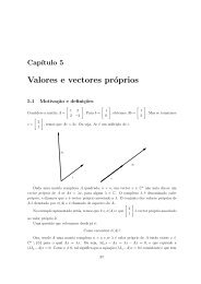
Campo <strong>de</strong> direções e uma solução <strong>de</strong> ẋ = sin(x)(1 − t 2 ).<br />
O teorema <strong>de</strong> Peano 3 4 afirma que, se o campo v(t, x) é contínuo, então existem sempre<br />
soluções locais (i.e. <strong>de</strong>fini<strong>da</strong>s em vizinhanças suficientemente pequenas <strong>do</strong> tempo inicial)<br />
<strong>do</strong> problema <strong>de</strong> Cauchy. O teorema <strong>de</strong> Picard-Lin<strong>de</strong>löf 5 afirma que, se o campo v(t, x) é<br />
contínuo e localmente Lipschitziano 6 (por exemplo, diferenciável <strong>de</strong> classe C 1 ) na variável<br />
x, então para ca<strong>da</strong> ponto (t 0 , x 0 ) ∈ T × X passa uma única solução com condição inicial<br />
x(t 0 ) = x 0 .<br />
• Esboce o campo <strong>de</strong> direções <strong>da</strong>s EDOs<br />
ẋ = t ẋ = −x + t ẋ = sin(t)<br />
e conjeture sobre o comportamento qualitativo <strong>da</strong>s soluções.<br />
3 G. Peano, Sull’integrabilità <strong>de</strong>lle equazioni differenziali <strong>de</strong>l primo ordine, Atti Accad. Sci. Torino 21 (1886),<br />
677-685.<br />
4 G. Peano, Demonstration <strong>de</strong> l’intégrabilité <strong>de</strong>s équations différentielles ordinaires, Mathematische Annalen 37<br />
(1890) 182-228.<br />
5 M. E. Lin<strong>de</strong>löf, Sur l’application <strong>de</strong> la métho<strong>de</strong> <strong>de</strong>s approximations successives aux équations différentielles<br />
ordinaires du premier ordre, Comptes rendus heb<strong>do</strong>ma<strong>da</strong>ires <strong>de</strong>s séances <strong>de</strong> l’Académie <strong>de</strong>s sciences 114 (1894),<br />
454-457.<br />
6 A função f : U → R m é Lipschitziana no <strong>do</strong>mínio U ⊂ R n se<br />
∃ L > 0 t.q. ‖f(x) − f(y)‖ ≤ L · ‖x − y‖ ∀ x, y ∈ U .
1<br />
EQUAÇÕES DIFERENCIAIS ORDINÁRIAS 7<br />
• A função x(t) = t 3 é solução <strong>da</strong> equação diferencial ẋ = 3x 2/3 com condição inicial<br />
x(0) = 0 E a função x(t) = 0 <br />
• Determine uma equação diferencial <strong>de</strong> primeira or<strong>de</strong>m e uma equação diferencial <strong>de</strong><br />
segun<strong>da</strong> or<strong>de</strong>m que admitam como solução a Gaussiana ϕ(t) = e −t2 /2 .<br />
5. (soluções <strong>de</strong> Chandrasekhar <strong>da</strong> equação <strong>de</strong> Lane-Em<strong>de</strong>n) Um mo<strong>de</strong>lo <strong>do</strong> perfil <strong>de</strong> equilíbrio<br />
hidrostático <strong>de</strong> uma estrela é a equação <strong>de</strong> Lane-Em<strong>de</strong>n<br />
(<br />
1 d<br />
ξ 2 ξ 2 dθ )<br />
= −θ p ,<br />
dξ dξ<br />
on<strong>de</strong> ξ ≥ 0 é uma “distância adimensional” <strong>do</strong> centro <strong>da</strong> estrela, θ(ξ) é proporcional à<br />
<strong>de</strong>nsi<strong>da</strong><strong>de</strong>, e p é um parâmetro que <strong>de</strong>pen<strong>de</strong> <strong>da</strong> equação <strong>de</strong> esta<strong>do</strong> P = Kρ 1+1/p <strong>do</strong> gás que<br />
forma a estrela. O problema físico é <strong>de</strong>terminare a solução com condições iniciais θ(0) = 1 e<br />
dθ/dξ(0) = 0, e o menor zero <strong>de</strong> θ(ξ) com ξ > 0 é interpreta<strong>do</strong> como sen<strong>do</strong> o raio <strong>da</strong> estrela.<br />
• Verifique que 7<br />
θ(ξ) = 1 − 1 6 ξ2 ,<br />
θ(ξ) = sin ξ<br />
ξ<br />
1<br />
e θ(ξ) = √<br />
1 + 1 3 ξ2<br />
são soluções <strong>da</strong> equação <strong>de</strong> Lane-Em<strong>de</strong>n quan<strong>do</strong> p = 0, 1 e 5, respetivamente.<br />
6. (campos <strong>de</strong> vetores e EDOs autónomas) Um campo <strong>de</strong> vetores v : X → R n no espaço <strong>de</strong> fases<br />
X ⊂ R n <strong>de</strong>fine uma equação diferencial ordinária autónoma (que não <strong>de</strong>pen<strong>de</strong> explicitamente<br />
<strong>do</strong> tempo, como to<strong>da</strong>s as leis fun<strong>da</strong>mentais <strong>da</strong> física)<br />
ẋ = v(x) .<br />
As imagens x(I) = {x(t) com t ∈ I} ⊂ X <strong>da</strong>s soluções/trajetórias x : I → X no espaço<br />
<strong>de</strong> fases são ditas órbitas, ou curvas <strong>de</strong> fases, <strong>do</strong> sistema autónomo. Se x ∈ X é um ponto<br />
singular <strong>do</strong> campo, i.e. um ponto on<strong>de</strong> v(x) = 0, então o caminho constante x(t) = x ∀t ∈ R<br />
é uma solução, dita solução <strong>de</strong> equilíbrio, ou estacionária.<br />
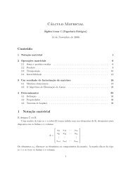
Campo <strong>de</strong> vetores e uma curva <strong>de</strong> fases <strong>do</strong> pêndulo com atrito,<br />
˙q = p, ṗ = − sin(q) − p/2.<br />
• Esboce o campo <strong>de</strong> direções e o campo <strong>de</strong> vetores <strong>da</strong>s EDOs autónomas<br />
ẋ = −x ẋ = x − 1 ẋ = x(1 − x)<br />
ẋ = (x − 1)(x − 2)(x − 3) ẋ = (x − 1) 2 (x − 2) 2<br />
{ { { ˙q = p<br />
˙q = 2q<br />
˙q = q − p<br />
ṗ = −q ṗ = −p/2 ṗ = p − q<br />
<strong>de</strong>termine as soluções <strong>de</strong> equilíbrio, e conjeture sobre o comportamento qualitativo <strong>da</strong>s<br />
(outras) soluções.<br />
7 Subrahmanyan Chandrasekhar, An Introduction to the Study of Stellar Structure, Dover, 1958.
1<br />
EQUAÇÕES DIFERENCIAIS ORDINÁRIAS 8<br />
7. (campos completos e fluxos <strong>de</strong> fases) Seja v : X ⊂ R n → R n um campo <strong>de</strong> vetores <strong>de</strong>fini<strong>do</strong><br />
num <strong>do</strong>mínio X ⊂ R n (ou numa varie<strong>da</strong><strong>de</strong> diferenciável). Se por ca<strong>da</strong> ponto x 0 ∈ X<br />
<strong>do</strong> espaço <strong>de</strong> fases passa uma e uma única solução global (ou seja, <strong>de</strong>fini<strong>da</strong> para to<strong>do</strong>s os<br />
tempos) ϕ : R → X, t ↦→ ϕ(t), com condição inicial ϕ(0) = x 0 , então o campo <strong>de</strong> vetores é dito<br />
completo. Um campo completo <strong>de</strong>fine/gera um fluxo <strong>de</strong> fases, um grupo <strong>de</strong> transformações<br />
Φ t = e tv : X → X, com t ∈ R, tais que<br />
Φ t ◦ Φ s = Φ t+s e Φ 0 = id X ∀ t, s, ∈ R .<br />
O ponto Φ t (x 0 ) é o esta<strong>do</strong> no tempo t <strong>da</strong> solução que passa por x 0 no instante 0. Vice-versa,<br />
um fluxo <strong>de</strong> fases diferenciável <strong>de</strong>fine um campo <strong>de</strong> vetores<br />
Φ t (x) − x<br />
v(x) := lim ,<br />
t→0 t<br />
dito “gera<strong>do</strong>r infinitesimal” <strong>do</strong> grupo <strong>de</strong> transformações. As curvas t ↦→ Φ t (x 0 ) são as soluções<br />
<strong>de</strong> ẋ = v(x) com condição inicial x(0) = x 0 .<br />
• Determine os campos <strong>de</strong> vetores que geram os seguintes fluxos no plano R 2<br />
Φ t (x, y) = (e λt x , e µt y)<br />
Φ t (x, y) = (cos(t) x − sin(t) y , sin(t) x + cos(t) y)<br />
Φ t (x, y) = (x + ty , y)<br />
8. (quase to<strong>da</strong>s as EDOs têm or<strong>de</strong>m um!) A EDO <strong>de</strong> or<strong>de</strong>m n ≥ 2 (resolúvel para a n-ésima<br />
<strong>de</strong>riva<strong>da</strong>)<br />
y (n) = F<br />
(t, y, ẏ, ÿ, ..., y (n−1))<br />
para o observável y(t) ∈ R é equivalente à EDO (ou sistema <strong>de</strong> EDOs) <strong>de</strong> primeira or<strong>de</strong>m<br />
ẋ = v (t, x)<br />
para o observável x = (x 1 , x 2 , ..., x n ) ∈ R n <strong>de</strong>fini<strong>do</strong> por<br />
x 1 := y x 2 := ẏ x 3 := ÿ ... x n := y (n−1) ,<br />
on<strong>de</strong> o campo <strong>de</strong> direções é v(t, x) := (x 2 , ..., x n−1 , F (t, x 1 , x 2 , ..., x n )).<br />
• Determine os sistemas <strong>de</strong> ODEs <strong>de</strong> or<strong>de</strong>m 1 que traduzem as seguintes ODEs <strong>de</strong> or<strong>de</strong>m<br />
> 1<br />
ẍ = −x ẍ + ẋ = 0 ẍ + ẋ + x = 0<br />
...<br />
ẍ = t − x ẍ + ẋ + x = 0 x = x
2<br />
INTEGRAÇÃO NUMÉRICA E SIMULAÇÕES* 9<br />
2 Integração numérica e simulações*<br />
1. (méto<strong>do</strong> <strong>de</strong> Euler) Consi<strong>de</strong>re o problema <strong>de</strong> simular as soluções <strong>da</strong> EDO ẋ = v(t, x). O<br />
méto<strong>do</strong> <strong>de</strong> Euler consiste em utilizar recursivamente a aproximação linear<br />
x(t + dt) ≃ x(t) + v(t, x) · dt ,<br />
<strong>da</strong><strong>do</strong> um “passo” dt suficientemente pequeno. Portanto, a solução x(t n ), nos tempos t n =<br />
t 0 + n · dt, com condição inicial x(t 0 ) = x 0 é estima<strong>da</strong> pela sucessão (x n ) n∈N0 <strong>de</strong>fini<strong>da</strong><br />
recursivamente por<br />
x n+1 = x n + v(t n , x n ) · dt .<br />
Numa linguagem como c++ ou Java, o ciclo para obter uma aproximação <strong>de</strong> x(t), <strong>da</strong><strong>do</strong><br />
x(t 0 ) = x, é<br />
while (time < t)<br />
{<br />
x += v(time, x) * dt ;<br />
time += dt ;<br />
}<br />
• Consi<strong>de</strong>re a equação diferencial<br />
ẋ = x<br />
com condição inicial x(0) = 1. Mostre que, se o passo é dt = ε e o tempo final é t = nε<br />
com n ∈ N, então o méto<strong>do</strong> <strong>de</strong> Euler fornece a aproximação<br />
x(t) ≃ x n = (1 + ε) n<br />
on<strong>de</strong> n = t/ε é o número <strong>de</strong> passos. Deduza que, no limite quan<strong>do</strong> o passo ε → 0, as<br />
aproximações convergem para a solução e t , pois<br />
(<br />
lim (1 +<br />
ε→0 ε)t/ε = lim 1 + t ) n<br />
n→∞ n<br />
• Simule a solução <strong>da</strong> EDO ẋ = (1 − 2t) x com condição inicial x(0) = 1. Compare o<br />
resulta<strong>do</strong> com o valor exacto x(t) = e t−t2 , usan<strong>do</strong> passos diferentes, por exemplo 0.01,<br />
0.001, 0.0001 ...<br />
• Aproxime, usan<strong>do</strong> o méto<strong>do</strong> <strong>de</strong> Euler, a solução <strong>do</strong> oscila<strong>do</strong>r harmónico<br />
{ ˙q = p<br />
ṗ = −q<br />
com condição inicial q(0) = 1 e p(0) = 0. Compare o valor <strong>de</strong> q(1) com o valor exacto<br />
q(1) = cos(1), usan<strong>do</strong> passos diferentes, por exemplo 0.1, 0.01, 0.001, 0.0001 ...<br />
2. (méto<strong>do</strong> RK-4) O méto<strong>do</strong> <strong>de</strong> Runge-Kutta (<strong>de</strong> or<strong>de</strong>m) 4 para simular a solução <strong>de</strong><br />
ẋ = v(t, x) com condição inicial x(t 0 ) = x 0<br />
consiste em escolher um “passo” dt, e aproximar x(t 0 + n · dt) com a sucessão (x n ) <strong>de</strong>fini<strong>da</strong><br />
recursivamente por<br />
x n+1 = x n + dt<br />
6 (k 1 + 2k 2 + 2k 3 + k 4 )<br />
on<strong>de</strong> t n = t 0 + n · dt, e os coeficientes k 1 , k 2 , k 3 e k 4 são <strong>de</strong>fini<strong>do</strong>s recursivamente por<br />
k 1 = v(t n , x n )<br />
k 2 = v ( t n + dt<br />
2 , x n + dt<br />
2 · k )<br />
1<br />
k 3 = v ( t n + dt<br />
2 , x n + dt<br />
2 · k )<br />
2<br />
• Implemente um código para simular sistemas <strong>de</strong> EDOs usan<strong>do</strong> o méto<strong>do</strong> RK-4.<br />
k 4 = v(t n + dt, x n + dt · k 3 )
2<br />
INTEGRAÇÃO NUMÉRICA E SIMULAÇÕES* 10<br />
3. (simulações com software proprietário) Existem software proprietários que permitem resolver<br />
analiticamente, quan<strong>do</strong> possível, ou fazer simulações numéricas <strong>de</strong> equações diferenciais<br />
ordinarias e parciais. Por exemplo, a função o<strong>de</strong>45 <strong>do</strong> MATLAB R○ , ou a função NDSolve <strong>do</strong><br />
Mathematica R○ , calculam soluções aproxima<strong>da</strong>s <strong>de</strong> EDOs ẋ = v(t, x) utilizan<strong>do</strong> variações <strong>do</strong><br />
méto<strong>do</strong> <strong>de</strong> Runge-Kutta.<br />
• Verifique se os PC <strong>do</strong> seu <strong>Departamento</strong>/<strong>da</strong> sua Universi<strong>da</strong><strong>de</strong> têm accesso a um <strong>do</strong>s<br />
software proprietários MATLAB R○ ou Mathematica R○ .<br />
• Em caso afirmativo, apren<strong>da</strong> a usar as funções o<strong>de</strong>45 ou NDSolve.<br />
Por exemplo, o pêndulo com atrito po<strong>de</strong> ser simula<strong>do</strong>, no Mathematica R○ , usan<strong>do</strong> as<br />
instruções<br />
s = NDSolve[{x’[t] == y[t], y’[t] == -Sin[x[t]] - 0.7 y[t],<br />
x[0] == y[0] == 1}, {x, y}, {t, 20}]<br />
ParametricPlot[Evaluate[{x[t], y[t]} /. s], {t, 0, 20}]<br />
O resulta<strong>do</strong> é<br />
0.2<br />
0.1<br />
0.3 0.2 0.1 0.1 0.2 0.3<br />
0.1<br />
0.2
3 TEOREMAS DE EXISTÊNCIA E UNICIDADE* 11<br />
3 Teoremas <strong>de</strong> existência e unici<strong>da</strong><strong>de</strong>*<br />
1. (iterações <strong>de</strong> Picard) Uma função diferenciável t ↦→ ϕ(t), <strong>de</strong>fini<strong>da</strong> num intervalo I ⊂ R e com<br />
valores num <strong>do</strong>mínio X ⊂ R n , é solução <strong>da</strong> equação diferencial ẋ = v(t, x) com condição<br />
inicial ϕ(t 0 ) = x 0 se e só se<br />
∫ t<br />
ϕ(t) = x 0 + v (s, ϕ(s)) ds ,<br />
t 0<br />
ou seja, se ϕ(t) é um ponto fixo <strong>do</strong> mapa <strong>de</strong> Picard P : C(I, X) → C(I, X), que envia uma<br />
função φ(t) na função<br />
(Pφ) (t) := x 0 + ∫ t<br />
t 0<br />
v (s, φ(s)) ds .<br />
Se a sucessão <strong>de</strong> funções φ, Pφ, P 2 φ := P (Pφ) , . . . , P n φ := P ( P n−1 φ ) , . . . , obti<strong>da</strong>s<br />
iteran<strong>do</strong> o mapa <strong>de</strong> Picard a partir <strong>de</strong> uma função inicial φ, é convergente (numa topologia<br />
apropria<strong>da</strong> <strong>de</strong>fini<strong>da</strong> num subespaço C ⊂ C(I, X) := {φ : I → X contínua} tal que P : C → C<br />
seja contínua), então o limite x(t) = lim n→∞ (P n φ) (t) é um ponto fixo <strong>do</strong> mapa <strong>de</strong> Picard,<br />
e portanto uma solução <strong>da</strong> equação diferencial ẋ = v(t, x) com a condição inicial <strong>da</strong><strong>da</strong><br />
x(t 0 ) = x 0 .<br />
• Se o campo <strong>de</strong> veloci<strong>da</strong><strong>de</strong>s apenas <strong>de</strong>pen<strong>de</strong> <strong>do</strong> tempo, então o mapa <strong>de</strong> Picard envia<br />
to<strong>da</strong> função inicial φ(t) na solução<br />
<strong>da</strong> EDO simples ẋ = v(t) com x(t 0 ) = x 0 .<br />
∫ t<br />
(Pφ) (t) = x 0 + v (s) ds<br />
t 0<br />
• Suppose you want to solve ẋ = x with initial condition x(0) = 1. You start with the<br />
guess φ(t) = 1, and then compute<br />
(Pφ) (t) = 1+t<br />
(<br />
P 2 φ ) (t) = 1+t+ 1 2 t2 . . . (P n φ) (t) = 1+t+ 1 2 t2 +· · ·+ 1 n! tn<br />
Hence the sequence converges (uniformly on boun<strong>de</strong>d intervals) to the Taylor series of<br />
the exponential function<br />
which is the solution we already knew.<br />
(P n φ) (t) → 1 + t + 1 2 t2 + · · · + 1 n! tn + ... = e t ,<br />
2. (contrações e teorema <strong>de</strong> ponto fixo <strong>de</strong> Banach) Seja (X, d) um espaço métrico. Uma transformação<br />
f : X → X é uma contração (ou λ-contração se é importante lembrar o valor <strong>de</strong><br />
λ) se é Lipschitz e tem constante <strong>de</strong> Lipschitz λ < 1, ou seja, se existe 0 ≤ λ < 1 tal que<br />
para to<strong>do</strong>s x, x ′ ∈ X<br />
d(f(x), f(x ′ )) ≤ λ · d(x, x ′ ) .<br />
As trajetórias <strong>da</strong> transformação f : X → X são as sucessões (x n ) <strong>de</strong>fini<strong>da</strong>s recursivamente<br />
por x n+1 = f(x n ), se n ≥ 0, a partir <strong>de</strong> uma condição inicial x 0 ∈ X. Os pontos fixos <strong>de</strong> f<br />
são os pontos p ∈ X tas que f(p) = p.<br />
O princípio <strong>da</strong>s contrações (a.k.a. teorema <strong>de</strong> ponto fixo <strong>de</strong> Banach) afirma que “to<strong>da</strong>s as trajetórias<br />
<strong>de</strong> uma contração f : X → X são sucesssões <strong>de</strong> Cauchy, e a distância entre ca<strong>da</strong> duas<br />
trajetórias diminue exponencialmente no tempo. Em particular, se X é completo, então f<br />
admite um único ponto fixo p, e a trajetória <strong>de</strong> to<strong>do</strong> ponto x ∈ X converge exponencialmente<br />
para o ponto fixo, i.e. f n (x) → p quan<strong>do</strong> n → ∞”.<br />
Demonstração. Seja f : X → X uma λ-contração. Seja x 0 ∈ X um ponto arbitrário, e seja<br />
(x n) a sua trajetória, ou seja, a sucessão <strong>de</strong>fini<strong>da</strong> recursivamente por x n+1 = f(x n). Usan<strong>do</strong>
3 TEOREMAS DE EXISTÊNCIA E UNICIDADE* 12<br />
k-vezes a contrativi<strong>da</strong><strong>de</strong> ve-se que d (x k+1 , x k ) ≤ d(x 1 , x 0 ) · λ k , e portanto que<br />
d(x n+k , x n)<br />
≤<br />
k−1 X<br />
k−1 X<br />
d(x n+j+1 , x n+j ) ≤ d(x 1 , x 0 ) · λ n+j<br />
j=0<br />
≤ d(x 1 , x 0 ) · λ n ·<br />
j=0<br />
∞X<br />
λ j ≤<br />
λn<br />
1 − λ · d(x 1, x 0 ) .<br />
j=0<br />
Em particular, (x n) é uma sucessão <strong>de</strong> Cauchy. O limite p = lim n→∞ x n, que existe se X<br />
é completo, é um ponto fixo <strong>de</strong> f, porque f é contínua. Se p e p ′ são pontos fixos, então<br />
d(p, p ′ ) = d(f(p), f(p ′ )) ≤ λd(p, p ′ ) com λ < 1 implica que d(p, p ′ ) = 0, o que mostra que o ponto<br />
fixo é único. Usan<strong>do</strong> a contrativi<strong>da</strong><strong>de</strong> também ve-se que d(x n, p) ≤ λ n · d(x 0 , p), ou seja que a<br />
convergência x n → p é exponencial.<br />
• Utilize o teorema <strong>do</strong> valor médio para mostrar que uma função f : R n → R n <strong>de</strong> classe<br />
C 1 é uma contração sse existe λ < 1 tal que |f ′ (x)| ≤ λ para to<strong>do</strong> x ∈ R n .<br />
• Mostre que uma transformação f : X → X tal que<br />
d(f(x), f(x ′ )) < d(x, x ′ )<br />
para to<strong>do</strong>s x, x ′ ∈ X distintos po<strong>de</strong> não ter pontos fixos, mesmo se o espaço métrico X<br />
for completo.<br />
3. (teorema <strong>de</strong> Picard-Lin<strong>de</strong>löf 8 .) Seja v(t, x) um campo <strong>de</strong> veloci<strong>da</strong><strong>de</strong>s contínuo <strong>de</strong>fini<strong>do</strong> num<br />
<strong>do</strong>mínio D <strong>do</strong> espaço <strong>de</strong> fases extendi<strong>do</strong> R×X. Se v é localmente Lipschitziana (por exemplo,<br />
diferenciável com continui<strong>da</strong><strong>de</strong>) com respeito a segun<strong>da</strong> variável x ∈ X ⊂ R n , então existe<br />
uma e uma única solução local <strong>da</strong> equação diferencial ẋ = v(t, x) que passa por ca<strong>da</strong> ponto<br />
(t 0 , x 0 ) ∈ D.<br />
Proof. In<strong>de</strong>ed, choose a sufficiently small rectangular neighborhood I × B = [t 0 − ε, t 0 + ε] ×<br />
B δ (x 0 ) around (t 0 , x 0 ), where B = B δ (x 0 ) <strong>de</strong>notes the closed ball with center x 0 and radius<br />
δ in X. There follows from continuity of v that there exists K such that |v(t, x)| ≤ K for any<br />
(t, x) ∈ I × B. There follows from the local Lipschitz condition for v that there exists M such<br />
that |v(t, x) − v(t, y)| ≤ M|x − y| for any t ∈ I and any x, y ∈ B. Now restrict, if nee<strong>de</strong>d, the<br />
(radius of the) interval I in such a way to get both the inequalities Kε ≤ δ and Mε < 1. Let<br />
C = C 0 (I, B) be the space of continuous functions t ↦→ φ(t) sending I into B. Equipped with<br />
the sup norm ‖φ − ϕ‖ ∞ := sup t∈I |φ(t) − ϕ(t)| this is a complete space. One verifies that the<br />
Picard’s map sends C into C, since<br />
Z t<br />
| (Pφ) (t) − x 0 | ≤ |v (s, φ(s)) | ds ≤ Kε ≤ δ .<br />
t 0<br />
Finally, given two functions φ, ϕ ∈ C, one sees that<br />
Z t<br />
| (Pφ) (t) − (Pϕ) (t)| ≤ |v (s, φ(s)) − v (s, ϕ(s)) | ds ≤ Mε · sup |φ(t) − ϕ(t)| ,<br />
t 0 t∈I<br />
hence ‖Pφ − Pϕ‖ ∞ < Mε · ‖φ − ϕ‖ ∞. Since λ := Mε < 1, this proves that the Picard’s map is<br />
a contraction and the Banach fixed point theorem allows to conclu<strong>de</strong>.<br />
4. (lema <strong>de</strong> Gromwall 9 ) Let φ(t) and ψ(t) be two non-negative real valued functions <strong>de</strong>fined in<br />
the interval [a, b], and assume that<br />
φ(t) ≤ K +<br />
∫ t<br />
for any a ≤ t ≤ b and some constant K ≥ 0. Then<br />
a<br />
ψ(s)φ(s) ds<br />
φ(t) ≤ Ke R t<br />
a ψ(s) ds .<br />
8 M. E. Lin<strong>de</strong>löf, Sur l’application <strong>de</strong> la métho<strong>de</strong> <strong>de</strong>s approximations successives aux équations différentielles<br />
ordinaires du premier ordre, Comptes rendus heb<strong>do</strong>ma<strong>da</strong>ires <strong>de</strong>s séances <strong>de</strong> l’Académie <strong>de</strong>s sciences 114 (1894),<br />
454-457.<br />
9 T.H. Gronwall, Note on the <strong>de</strong>rivative with respect to a parameter of the solutions of a system of differential<br />
equations, Ann. of Math 20 (1919), 292-296.
3 TEOREMAS DE EXISTÊNCIA E UNICIDADE* 13<br />
Proof. In<strong>de</strong>ed, assume that K > 0. Define Φ(t) := K + R t<br />
a ψ(s)φ(s) ds and observe that<br />
Φ(a) = K > 0, hence Φ(t) > 0 for all a ≤ t ≤ b. The logarithmic <strong>de</strong>rivative is<br />
d<br />
ψ(t)φ(t)<br />
log Φ(t) = ≤ ψ(t)<br />
dt Φ(t)<br />
where we used the hypothesis φ(t) ≤ Φ(t). Integrating the inequality we get, for a ≤ t ≤ b,<br />
Z t<br />
log Φ(t) ≤ Φ(a) + ψ(s) ds .<br />
a<br />
Exponentiation gives the result, since<br />
φ(t) ≤ Φ(t) ≤ K · eR ta<br />
ψ(s) ds .<br />
The case K = 0 follows taking the limit of the above inequalities along a sequence of K n > 0<br />
<strong>de</strong>creasing to zero.<br />
5. (<strong>de</strong>pen<strong>de</strong>nce on initial <strong>da</strong>ta and parameters)
4 EDOS SIMPLES E AUTÓNOMAS NA RETA 14<br />
4 EDOs simples e autónomas na reta<br />
1. (integração <strong>de</strong> EDOs simples) O teorema (fun<strong>da</strong>mental <strong>do</strong> cálculo) <strong>de</strong> Newton e Leibniz 10<br />
afirma que a <strong>de</strong>riva<strong>da</strong> <strong>do</strong> integral in<strong>de</strong>fini<strong>do</strong> F (t) := ∫ t<br />
f(s) ds <strong>de</strong> uma função contínua f(t)<br />
a<br />
existe e é igual a F ′ (t) = f(t). Portanto, se v(t) é um campo <strong>de</strong> direções contínuo, a solução<br />
<strong>da</strong> EDO<br />
ẋ = v(t)<br />
com condição inicial x(t 0 ) = x 0 é <strong>de</strong>termina<strong>da</strong> por meio <strong>de</strong> uma integração, ou seja,<br />
ẋ = v(t) , x(t 0 ) = x 0 ⇒ x(t) = x 0 + ∫ t<br />
t 0<br />
v(s)ds<br />
(<strong>do</strong>n<strong>de</strong> a tradição <strong>de</strong> dizer “integrar” uma equação diferencial em vez <strong>de</strong> “resolver”). Se x(t)<br />
é solução <strong>de</strong> ẋ = v(t), então também x(t) + c é solução, ∀c ∈ R.<br />
• Integre as seguintes EDOs, <strong>de</strong>fini<strong>da</strong>s em oportunos intervalos <strong>de</strong> tempo<br />
ẋ = 2 − t + 3t 2 + 5t 6 ẋ = e −t ẋ = cos(3t) ẋ = 1/t<br />
2. (foguetão) Se um foguetão <strong>de</strong> massa m(t) no espaço vazio (ou seja, sem forças gravitacionais!)<br />
expulsa combustível a uma veloci<strong>da</strong><strong>de</strong> relativa constante −V e a uma taxa constante ṁ = −α,<br />
então a sua trajetória num referencial inercial é mo<strong>de</strong>la<strong>da</strong> pela equação <strong>de</strong> Newton<br />
d<br />
(mv) = α(V − v) , ou seja , ṁv + m ˙v = α(V − v) .<br />
dt<br />
• Resolva a EDO ṁ = −α para a massa <strong>do</strong> foguetão, com massa inicial m(0) = m 0 > 0,<br />
e substitua o resulta<strong>do</strong> na equação <strong>de</strong> Newton, obten<strong>do</strong><br />
(<strong>de</strong>s<strong>de</strong> que 0 ≤ t < m 0 /α).<br />
˙v =<br />
αV<br />
m 0 − αt<br />
• Calcule a trajetória <strong>do</strong> foguetão com veloci<strong>da</strong><strong>de</strong> inicial v(0) = v 0 e posição inicial q(0) =<br />
0, váli<strong>da</strong> para tempos t inferiores ao tempo necessário para acabar o combustível.<br />
3. (campos <strong>de</strong> vetores e EDOs autónomas na reta) Um campo <strong>de</strong> vetores v : X → R, <strong>de</strong>fini<strong>do</strong><br />
num intervalo X ⊂ R, <strong>de</strong>fine uma EDO autónoma<br />
ẋ = v(x) .<br />
Se x 0 é um ponto singular <strong>de</strong> v(x), i.e. um ponto on<strong>de</strong> v(x 0 ) = 0, então x(t) = x 0 ∀t ∈ R<br />
é uma solução estacionária (ou <strong>de</strong> equilíbrio) <strong>da</strong> equação. Se x 0 é um ponto não singular<br />
<strong>do</strong> campo contínuo v(x), i.e. se v(x 0 ) ≠ 0, então uma solução local com condição inicial<br />
x(t 0 ) = x 0 po<strong>de</strong> ser <strong>de</strong>terminan<strong>da</strong> “separan<strong>do</strong> as variáveis”, ou seja, fazen<strong>do</strong><br />
integran<strong>do</strong> os <strong>do</strong>is membros, ∫ dx<br />
v(x) = ∫ dt. Ou seja,<br />
ẋ = v(x) , x(t 0 ) = x 0<br />
Se o campo v(x) é diferenciável, estas soluções são únicas.<br />
10 A solução <strong>do</strong> anagrama<br />
6acc<strong>da</strong>e13eff7i3l9n4o4qrr4s8t12vx<br />
⇒<br />
{<br />
∫ x<br />
x 0<br />
x(t) = x 0 se v(x 0 ) = 0<br />
dy<br />
v(y) = t − t 0 se v(x 0 ) ≠ 0<br />
dx<br />
v(x)<br />
= dt e<br />
conti<strong>do</strong> numa carta <strong>de</strong> Isaac Newton dirigi<strong>da</strong> a Gottfried Leibniz em 1677, é “Data aequatione quotcunque fluentes<br />
quantitates involvente fluxiones invenire et vice versa”.
4 EDOS SIMPLES E AUTÓNOMAS NA RETA 15<br />
Proof. In<strong>de</strong>ed, assume that the velocity field v is continuous and let J = (x − , x + ) be the<br />
maximal interval containing x 0 where v is different from zero. Define a function H : R × J → R<br />
as<br />
Z x dy<br />
H(t, x) = t − t 0 −<br />
x 0<br />
v(y) .<br />
If t ↦→ ϕ(t) is a solution of the Cauchy problem, then computation shows that d H (t, ϕ(t)) = 0<br />
dt<br />
for any time t. There follows that H is constant along the solutions of the Cauchy problem.<br />
Since H(t 0 , x 0 ) = 0, we conclu<strong>de</strong> that the graph of any solution belongs to the level set Σ =<br />
{(t, x) ∈ R × J s.t. H(t, x) = 0}. Now observe that H is continuously differentiable and that its<br />
differential dH = dt + dx/v(x) is never zero. Actually, both partial <strong>de</strong>rivatives ∂H/∂t and ∂H/∂x<br />
are always different from zero. Hence we can apply the implicit function theorem and conclu<strong>de</strong><br />
that the level set Σ is, in some neighborhood I × J of (t 0 , x 0 ), the graph of a unique differentiable<br />
function x ↦→ t(x), as well as the graph of a unique differentiable function t ↦→ x(t), the inverse<br />
of t, which solves the<br />
“<br />
Cauchy<br />
”<br />
problem: just compute the <strong>de</strong>rivative (using the inverse function<br />
theorem), ẋ(t) = 1/ dt<br />
dx (x(t)) = v(x), and check the initial condition. Observe that the function<br />
t(x) − t 0 has then the interpretation of the “time nee<strong>de</strong>d to go from x 0 to x”.<br />
Se x(t) é solução <strong>de</strong> ẋ = v(x), então também x(t − c) é solução, ∀c ∈ R (a física mo<strong>de</strong>la<strong>da</strong><br />
por uma EDO autónoma é invariante para translações no tempo).<br />
• Consi<strong>de</strong>re as seguintes EDOs autónomas<br />
ẋ = −3x ẋ = x − 1 ẋ = x 2 ẋ = √ x<br />
ẋ = (x − 1)(x − 2) ẋ = e x ẋ = (x − 1)(x − 2)(x − 3)<br />
<strong>de</strong>fini<strong>da</strong>s em intervalos convenientes. Encontre, caso existam, as soluções estacionárias.<br />
Desenhe os respectivos campos <strong>de</strong> vetores e conjeture sobre o comportamento <strong>da</strong>s<br />
soluções. Integre, quan<strong>do</strong> possível, as equações e calcule soluções. Determine, quan<strong>do</strong><br />
possível, umas fórmulas para a solução <strong>do</strong> problema <strong>de</strong> Cauchy comcondição inicial<br />
x(0) = x 0 e esboce a representação gráfica <strong>de</strong> algumas <strong>da</strong>s soluções encontra<strong>da</strong>s.<br />
4. (<strong>de</strong>caimento radioativo) A taxa <strong>de</strong> <strong>de</strong>caimento <strong>de</strong> matéria radioativa é proporcional à quanti<strong>da</strong><strong>de</strong><br />
<strong>de</strong> matéria existente, <strong>de</strong>s<strong>de</strong> que a amostra seja suficientemente gran<strong>de</strong>. Quer isto dizer<br />
que a quanti<strong>da</strong><strong>de</strong> N(t) <strong>de</strong> matéria radioativa existente no instante t satisfaz a lei<br />
Ṅ = −βN ,<br />
on<strong>de</strong> o parâmetro 1/β > 0 é a “vi<strong>da</strong> média” <strong>do</strong>s núcleos 11 .<br />
• Determine a solução com condição inicial N(0) = N 0 > 0.<br />
t → ∞<br />
O que acontece quan<strong>do</strong><br />
• O tempo <strong>de</strong> meia-vi<strong>da</strong> <strong>de</strong> uma matéria radioativa é o tempo τ necessário até a quanti<strong>da</strong><strong>de</strong><br />
<strong>de</strong> matéria se reduzir a meta<strong>de</strong> <strong>da</strong> quanti<strong>da</strong><strong>de</strong> inicial (ou seja, N(τ) = 1 2 N(0)).<br />
Mostre que o tempo <strong>de</strong> meia-vi<strong>da</strong> não <strong>de</strong>pen<strong>de</strong> <strong>da</strong> quanti<strong>da</strong><strong>de</strong> inicial N(0), e <strong>de</strong>termine<br />
a relação entre o tempo <strong>de</strong> meia-vi<strong>da</strong> τ e o parâmetro β.<br />
• O radiocarbono 14 C tem vi<strong>da</strong> média 1/β ≃ 8033 anos. Mostre como <strong>da</strong>tar um fóssil,<br />
assumin<strong>do</strong> que a proporção <strong>de</strong> radiocarbono num ser vivente é conheci<strong>da</strong> 12 .<br />
• Se a radiação solar produz radiocarbono na atmosfera terrestre a uma taxa constante<br />
α > 0, então a quanti<strong>da</strong><strong>de</strong> <strong>de</strong> radiocarbono na atmosfera segue a lei<br />
Ṅ = −βN + α .<br />
Verifique que a solução <strong>de</strong> equilíbrio é N = α/β. Mostre que N(t) → N quan<strong>do</strong><br />
t → ∞, in<strong>de</strong>pen<strong>de</strong>ntemente <strong>da</strong> condição inicial N(0) (consi<strong>de</strong>re a mu<strong>da</strong>nça <strong>de</strong> variável<br />
x(t) = N(t) − N).<br />
11 O tempo <strong>de</strong> vi<strong>da</strong> <strong>de</strong> ca<strong>da</strong> núcleo é mo<strong>de</strong>la<strong>do</strong> por uma variável aleatória exponencial X, com lei Prob(X ≤<br />
t) = 1 − e −βt se t ≥ 0, e 0 se t < 0, e média EX := R ∞<br />
0 t dProb(X ≤ t) = 1/β. A equação diferencial, quan<strong>do</strong> a<br />
quanti<strong>da</strong><strong>de</strong> N <strong>de</strong> núcleos é gran<strong>de</strong>, é uma consequência <strong>da</strong> lei <strong>do</strong>s gran<strong>de</strong>s números.<br />
12 J.R. Arnold and W.F. Libby, Age Determinations by Radiocarbon Content: Checks with Samples of Known<br />
Ages, Sciences 110 (1949), 1127-1151.
4 EDOS SIMPLES E AUTÓNOMAS NA RETA 16<br />
5. (atrito e tempo <strong>de</strong> relaxamento) O atrito po<strong>de</strong> ser mo<strong>de</strong>la<strong>do</strong> como sen<strong>do</strong> uma força proporcional<br />
e contrária à veloci<strong>da</strong><strong>de</strong>. Portanto, a equação <strong>de</strong> Newton (em dimensão 1) <strong>de</strong> uma<br />
partícula livre <strong>de</strong> massa m em presença <strong>de</strong> atrito é<br />
on<strong>de</strong> γ > 0 é o “coeficiente <strong>de</strong> atrito”.<br />
• Mostre que a veloci<strong>da</strong><strong>de</strong> v := ˙q satisfaz<br />
m¨q = −γ ˙q<br />
˙v = − 1 τ v<br />
on<strong>de</strong> τ = m/γ > 0 é um “tempo <strong>de</strong> relaxamento”. Resolva a equação <strong>da</strong><strong>da</strong> uma<br />
veloci<strong>da</strong><strong>de</strong> inicial v(0) = v 0 > 0. Deduza a trajectória q(t) com posição inicial q(0) = 0.<br />
• Mostre que a energia cinética T := 1 2 mv2 <strong>da</strong> partícula satisfaz<br />
˙ T = − 2 τ T ,<br />
e portanto <strong>de</strong>cresce exponencialmente com tempo <strong>de</strong> relaxamento τ/2.<br />
6. (paraquedista) Um mo<strong>de</strong>lo <strong>da</strong> que<strong>da</strong> <strong>de</strong> um paraquedista é<br />
m ˙v = −αv 2 − mg ,<br />
on<strong>de</strong> v(t) := ˙q(t), q(t) ∈ R é a altura no instante t, m > 0 é a massa, g ≃ 980 cm s −2<br />
é a aceleração <strong>da</strong> gravi<strong>da</strong><strong>de</strong> próximo <strong>da</strong> superfície terrestre, e α > 0 é uma constante que<br />
<strong>de</strong>pen<strong>de</strong> <strong>da</strong> atmosfera e <strong>do</strong> paraque<strong>da</strong> (um valor realístico é α ≃ 30 kg/m).<br />
• Mostre que a veloci<strong>da</strong><strong>de</strong> v(t) converge para o valor estacionário v = √ mg/α quan<strong>do</strong><br />
t → ∞.<br />
7. (crescimento exponencial) Um mo<strong>de</strong>lo <strong>do</strong> crescimento <strong>de</strong> uma população num meio ambiente<br />
ilimita<strong>do</strong> é<br />
Ṅ = λN ,<br />
on<strong>de</strong> N(t) é a quanti<strong>da</strong><strong>de</strong> <strong>de</strong> exemplares existentes no instante t, e λ > 0 (se α é a taxa <strong>de</strong><br />
natali<strong>da</strong><strong>de</strong> e β é a taxa <strong>de</strong> mortali<strong>da</strong><strong>de</strong>, então λ = α − β).<br />
• Determine a solução com condição inicial N(0) = N 0 > 0.<br />
t → ∞<br />
O que acontece quan<strong>do</strong><br />
• Se a população <strong>de</strong> uma bactéria duplica numa hora, quanto aumentará em duas horas<br />
• Se <strong>de</strong> uma população que cresce exponencialmente é retira<strong>da</strong> uma parte a uma taxa<br />
constante γ, então a população segue a lei<br />
Ṅ = λN − γ .<br />
Determine o esta<strong>do</strong> estacionário, e discuta o comportamento assimptótico <strong>da</strong>s outras<br />
soluções.<br />
8. (logística) Um mo<strong>de</strong>lo mais realista <strong>da</strong> dinâmica <strong>de</strong> uma população é <strong>da</strong><strong>do</strong> pela equação<br />
logística 13<br />
Ṅ = λ N (1 − N/M)<br />
on<strong>de</strong> a constante positiva M > 0 é a população máxima permiti<strong>da</strong> num <strong>da</strong><strong>do</strong> meio ambiente<br />
limita<strong>do</strong>. Note que Ṅ ≃ λN (e portanto o crescimento é exponencial) se N ≪ M, e que<br />
Ṅ → 0 (e portanto a população é constante) quan<strong>do</strong> N → M. A “população relativa”<br />
x(t) := N(t)/M satisfaz a equação logística “adimensional”<br />
ẋ = λ x (1 − x) .<br />
13 Pierre François Verhulst, Notice sur la loi que la population pursuit <strong>da</strong>ns son accroissement, Correspon<strong>da</strong>nce<br />
mathématique et physique 10 (1838), 113-121.
4 EDOS SIMPLES E AUTÓNOMAS NA RETA 17<br />
• Determine as soluções <strong>de</strong> equilíbrio <strong>da</strong> equação logística.<br />
• Verifique que a solução com condição inicial x(0) = x 0 ∈ (0, 1) é<br />
1<br />
x(t) = ( ) .<br />
1<br />
1 +<br />
x 0<br />
− 1 e −λt<br />
• Discuta o comportamento assimptótico <strong>da</strong>s soluções <strong>da</strong> equação logística.<br />
9. (crescimento super-exponencial) Um outro mo<strong>de</strong>lo <strong>de</strong> dinâmica <strong>de</strong> uma população em meio<br />
ilimita<strong>do</strong> é<br />
Ṅ = λN 2 ,<br />
ou seja, a taxa <strong>de</strong> crescimento é proporcional aos pares <strong>de</strong> indivíduos conti<strong>do</strong>s na população.<br />
• Determine a solução estacionária e a solução com condição inicial N(0) = N 0 > 0<br />
arbitrária.<br />
• Note que as soluções que <strong>de</strong>terminou não estão <strong>de</strong>fini<strong>da</strong>s para to<strong>da</strong> a recta real: este<br />
mo<strong>de</strong>lo prevê uma catástrofe (população infinita) após um intervalo <strong>de</strong> tempo finito!<br />
10. (fazer mo<strong>de</strong>los) Escreva equações diferenciais que mo<strong>de</strong>lem ca<strong>da</strong> uma <strong>da</strong>s seguintes situações.<br />
O que po<strong>de</strong> dizer sobre as soluções<br />
• A taxa <strong>de</strong> variação <strong>da</strong> temperatura <strong>de</strong> uma chávena <strong>de</strong> chá é proporcional à diferença<br />
entre a temperatura <strong>do</strong> quarto, suposta constante, e a temperatura <strong>do</strong> chá.<br />
• A veloci<strong>da</strong><strong>de</strong> vertical <strong>de</strong> um foguetão é inversamente proporcional à altura atingi<strong>da</strong>.<br />
• A taxa <strong>de</strong> crescimento <strong>da</strong> massa <strong>de</strong> um cristal cúbico é proporcional à sua superfície.<br />
• Uma esfera <strong>de</strong> gelo <strong>de</strong>rrete a uma taxa proporcional à sua superfície.<br />
• A taxa <strong>de</strong> crescimento <strong>de</strong> uma população <strong>de</strong> marcianos é proporcional ao número <strong>de</strong><br />
trios que é possível formar com a <strong>da</strong><strong>da</strong> população.<br />
• A taxa <strong>de</strong> crescimento <strong>do</strong> número <strong>de</strong> individuos infecta<strong>do</strong>s <strong>de</strong>ntro <strong>de</strong> uma população<br />
constante é proporcional ao número <strong>de</strong> individuos infecta<strong>do</strong>s e ao número <strong>de</strong> individuos<br />
ain<strong>da</strong> não infecta<strong>do</strong>s.
5 SISTEMAS CONSERVATIVOS* 18<br />
5 Sistemas conservativos*<br />
1. (constantes <strong>do</strong> movimento) Seja v : X ⊂ R n → R n , com coor<strong>de</strong>na<strong>da</strong>s v(x) = (v 1 (x), . . . , v n (x)),<br />
um campo <strong>de</strong> vetores que <strong>de</strong>fine a EDO autónoma<br />
ẋ = v(x)<br />
num espaço <strong>de</strong> fases X ⊂ R n . Os observáveis são as funções ϕ : X → R. Os observáveis que<br />
assumem valores ϕ(x(t)) constantes ao longo <strong>da</strong>s soluções x(t) <strong>de</strong> ẋ = v(x) são ditos constantes<br />
<strong>do</strong> movimento, ou integrais primeiros. Pela regra <strong>da</strong> ca<strong>de</strong>ia, o observável diferenciável<br />
ϕ : X → R é uma constante <strong>do</strong> movimento se e só se a <strong>de</strong>riva<strong>da</strong> <strong>de</strong> Lie <strong>de</strong> ϕ ao longo <strong>do</strong><br />
campo v é igual a zero, ou seja,<br />
para to<strong>do</strong>s os pontos x ∈ X.<br />
(£ v ϕ) (x) :=<br />
n∑<br />
k=1<br />
∂ϕ<br />
∂x k<br />
(x) · v k (x) = 0 .<br />
As órbitas/curvas <strong>de</strong> fases estão conti<strong>da</strong>s nas hiperfícies <strong>de</strong> nível Σ c := {x ∈ X t.q. ϕ(x) =<br />
c} <strong>da</strong>s constantes <strong>do</strong> movimento. Se o sistema admite k constantes <strong>do</strong> movimento in<strong>de</strong>pen<strong>de</strong>ntes<br />
ϕ 1 , ϕ 2 , . . . , ϕ k (ou seja, tais que os diferenciais dϕ i (x) são linearmente in<strong>de</strong>pen<strong>de</strong>ntes<br />
em ca<strong>da</strong> ponto x), então as órbitas <strong>do</strong> sistema estão conti<strong>da</strong>s nas interseções <strong>da</strong>s k hiperfícies<br />
<strong>de</strong> nível, umas sub-varie<strong>da</strong><strong>de</strong>s <strong>de</strong> co-dimensão k. Em particular, a existência <strong>de</strong> n − 1 constantes<br />
<strong>do</strong> movimento in<strong>de</strong>pen<strong>de</strong>ntes permite <strong>de</strong>terminar as órbitas.<br />
• Verifique que o sistema ẋ = Ax, on<strong>de</strong> A é uma matriz diagonal com <strong>de</strong>t A ≠ 0 (ou seja,<br />
to<strong>do</strong>s os valores próprios são ≠ 0) não admite constantes <strong>do</strong> movimento não triviais (i.e.<br />
constantes).<br />
2. (sistemas conservativos) [LL78] A trajetória t ↦→ r(t) ∈ R 3 <strong>de</strong> uma partícula <strong>de</strong> massa m > 0<br />
(suposta constante!) num campo <strong>de</strong> forças conservativo é mo<strong>de</strong>la<strong>da</strong> pela equação <strong>de</strong> Newton<br />
m¨r = F<br />
on<strong>de</strong> a força é F(r) = −∇U(r), e U(r) é um(a energia) potencial. Um sistema isola<strong>do</strong> <strong>de</strong><br />
N pontos materiais, com posições r α (t) ∈ R 3 e massas m α > 0, com α = 1, 2, . . . , N, é<br />
mo<strong>de</strong>la<strong>do</strong> pelas equações <strong>de</strong> Newton<br />
m α¨r α = F α<br />
α = 1, 2, . . . , N<br />
on<strong>de</strong> a força que atua sobre o α-ésimo ponto material é<br />
( ∂U<br />
F α = −∇ rα U := − , ∂U , ∂U )<br />
,<br />
∂x α ∂y α ∂z α<br />
menos o gradiente, com respeito às coor<strong>de</strong>na<strong>da</strong>s r α = (x α , y α , z α ), <strong>de</strong> uma energia potencial<br />
U(r 1 , r 2 , . . . , r N ). A energia cinética é<br />
K :=<br />
N∑<br />
α=1<br />
1<br />
2 m α‖v α ‖ 2<br />
on<strong>de</strong> v α = ṙ α é a veloci<strong>da</strong><strong>de</strong> <strong>do</strong> α-ésimo ponto material.<br />
• Verifique que a energia (energia cinética + energia potencial)<br />
E := K + U =<br />
N∑<br />
α=1<br />
1<br />
2 m α‖v α ‖ 2 + U (r 1 , r 2 , . . . , r N )<br />
é uma constante <strong>do</strong> movimento, ou seja, que d dtE = 0 ao longo <strong>da</strong>s trajetórias.
5 SISTEMAS CONSERVATIVOS* 19<br />
3. (mecânica lagrangiana e hamiltoniana) Um sistema mecânico é <strong>de</strong>scrito por um espaço <strong>da</strong>s<br />
configurações M ≃ R n (ou, em geral, uma varie<strong>da</strong><strong>de</strong> diferenciável), com coor<strong>de</strong>na<strong>da</strong>s locais<br />
q = (q 1 , q 2 , . . . , q n ) ∈ R n , e uma lagrangiana L : T M ≃ R n × R n → R, ou seja, uma função<br />
L(q, ˙q). Por exemplo, o espaço <strong>da</strong>s configurações <strong>de</strong> um sistema <strong>de</strong> N pontos materiais é o<br />
espaço <strong>do</strong>s vetores q = (r 1 , r 2 , . . . , r n ) ∈ R 3N , on<strong>de</strong> r α ∈ R 3 , com α = 1, 2, . . . , N, representa<br />
a posição <strong>do</strong> α-ésimo ponto. A lagrangiana é<br />
L(q, ˙q) = ∑ α<br />
m α<br />
2 ‖ṙ α‖ 2 − U(r 1 , r 2 , . . . , r α ) .<br />
A ação <strong>de</strong> uma trajetória [t 0 , t 1 ] ↦→ q(t) ∈ M entre a posição q(t 0 ) e a posição q(t 1 ) é o<br />
integral<br />
∫ t1<br />
S[t ↦→ q(t)] := L(q(t), ˙q(t)) dt .<br />
t 0<br />
O princípio <strong>de</strong> mínima ação (<strong>de</strong> Hamilton) afirma que as trajetórias físicas são os pontos<br />
críticos <strong>da</strong> ação. A variação δS, <strong>da</strong><strong>da</strong> uma variações infinitésimas q(t) + δq(t) <strong>da</strong> trajetória<br />
com δq(t 0 ) = δq(t 1 ) = 0, é <strong>da</strong><strong>da</strong> por<br />
∫ t1 ∑<br />
( ∂L<br />
δS =<br />
δq i (t) + ∂L )<br />
δ ˙q i (t) dt<br />
t 0<br />
∂q<br />
i i ∂ ˙q i<br />
∫ t1 ∑<br />
( ∂L<br />
=<br />
− d )<br />
∂L<br />
δq i (t) dt<br />
∂q i dt ∂ ˙q i<br />
t 0<br />
i<br />
(integran<strong>do</strong> por partes a segun<strong>da</strong> soma e usan<strong>do</strong> as condições <strong>de</strong> fronteira). Portanto, os<br />
pontos críticos <strong>da</strong> ação são as soluções <strong>da</strong>s equações <strong>de</strong> Euler-Lagrange<br />
( )<br />
d ∂L<br />
dt ∂ ˙q i<br />
= ∂L<br />
∂q i<br />
i = 1, 2, . . . , n .<br />
A forma linear p = (p 1 , p 2 . . . , p N ) = p 1 dq 1 + p 2 dq 2 + · · · + p n dq n ∈ TqM, ∗ <strong>de</strong> coor<strong>de</strong>na<strong>da</strong>s<br />
p i := ∂L/∂ ˙q i (q), é dito momento. O espaço X = T ∗ M ≃ R n × (R n ) ∗ , com coor<strong>de</strong>na<strong>da</strong>s<br />
(q, p), é dito espaço <strong>de</strong> fases <strong>do</strong> sistema mecânico. As equações <strong>de</strong> Euler-Lagrange são<br />
equivalentes às equações <strong>de</strong> Hamilton<br />
˙q i = ∂H<br />
∂p i<br />
ṗ i = − ∂H<br />
∂q i<br />
i = 1, 2, . . . , n ,<br />
on<strong>de</strong> a hamiltoniana <strong>do</strong> sistema, H : X → R, é a “transforma<strong>da</strong> <strong>de</strong> Legendre” <strong>da</strong> lagrangiana,<br />
<strong>de</strong>fini<strong>da</strong> por<br />
H (q, p) := sup (p · ˙q − L(q, ˙q))<br />
v<br />
= ∑ 1<br />
2m ‖p α‖ 2 + U (q) .<br />
α<br />
• O espaço <strong>da</strong>s configurações <strong>de</strong> um sistema <strong>de</strong> N pontos materiais é o espaço <strong>do</strong>s vetores<br />
q = (r 1 , r 2 , . . . , r n ) ∈ R 3N , on<strong>de</strong> r α ∈ R 3 , com α = 1, 2, . . . , N, representa a posição <strong>do</strong><br />
α-ésimo ponto. A lagrangiana é<br />
L(q, ˙q) = ∑ α<br />
m α<br />
2 ‖ṙ α‖ 2 − U(r 1 , r 2 , . . . , r α ) ,<br />
on<strong>de</strong> U é a energia potencial <strong>da</strong> interação. Verifique que as equações <strong>de</strong> Euler-Lagrange<br />
são equivalentes às equações <strong>de</strong> Newton m α r¨<br />
α = F α .<br />
• Mostre que a hamiltoniana é uma constante <strong>do</strong> movimento, ou seja, que<br />
d<br />
H(q(t), p(t)) = 0<br />
dt<br />
ao longo <strong>da</strong>s soluções <strong>da</strong>s equações <strong>de</strong> Hamilton. Deduza que as órbitas <strong>do</strong> sistema<br />
no espaço <strong>de</strong> fases X estão conti<strong>da</strong>s nas curvas/superfícies <strong>de</strong> nível {H(q, p) = c} <strong>da</strong><br />
hamiltoniana.
5 SISTEMAS CONSERVATIVOS* 20<br />
4. (Legendre transform) The Legendre transform of a real-valued function f : R n → R is the<br />
real-valued function F : (R n ) ′ → R <strong>de</strong>fined by<br />
F (p) := sup (〈p, x〉 − f(x))<br />
x<br />
If f(x) is differentiable, the extremum is attained at p = f ′ (x), and this is a maximum if<br />
f(x) is convex, i.e. if f ′′ (x) > 0.<br />
• Find the Legendre transform of<br />
f(x) = λx 2<br />
f(x) = e x<br />
f(x) = 1 2 〈x, Ax〉 x ∈ Rn , A ∈ GL n (R) symmetric<br />
5. (one-dimensional Newtonian motion in a time in<strong>de</strong>pen<strong>de</strong>nt force field) The one-dimensional<br />
motion of a particle of mass m subject to a force F (x) that <strong>do</strong>es not <strong>de</strong>pend on time is<br />
<strong>de</strong>scribed by the Newton equation<br />
mẍ = − dU<br />
dx (x) ,<br />
where the potential U(x) = − ∫ F (x)dx is some primitive of the force. The total energy<br />
E (x, ẋ) = 1 2 mẋ2 + U(x)<br />
(which of course is <strong>de</strong>fined up to an arbitrary additive constant) of the system is a constant<br />
of the motion, i.e. is constant along solutions of the Newton equation. In particular, once a<br />
value E of the energy is given (<strong>de</strong>pending on the initial conditions), the motion takes place<br />
in the region where U(x) ≤ E, since the kinetic energy 1 2 mẋ2 is non-negative. Conservation<br />
of energy allows to reduce the problem to the first or<strong>de</strong>r ODE<br />
ẋ 2 = 2 (E − U(x)) ,<br />
m<br />
which has the unpleasant feature to be quadratic in the velocity ẋ. Meanwhile, if we are<br />
interested in a one-way trajectory going from some x 0 to x, say with x > x 0 , we may solve<br />
for ẋ and find the first or<strong>de</strong>r autonomous ODE<br />
√<br />
2<br />
ẋ = (E − U(x)) .<br />
m<br />
There follows that the time nee<strong>de</strong>d to go from x 0 to x is<br />
t(x) =<br />
∫ x<br />
x 0<br />
dy<br />
√<br />
.<br />
2<br />
m (E − U(y))<br />
The inverse function of the above t(x) will<br />
√<br />
give the trajectory x(t) with initial position<br />
2<br />
x(0) = x 0 and initial positive velocity ẋ(0) =<br />
m (E − U(x 0)), at least for sufficiently small<br />
times t.<br />
6. (pêndulo matemático) A equação <strong>de</strong> Newton que mo<strong>de</strong>la as oscilações <strong>de</strong> um pêndulo é<br />
¨θ = −ω 2 sin(θ) ,<br />
on<strong>de</strong> ω = √ g/l , g ≃ 980 cm s −2 é a aceleração gravitacional, l o comprimento <strong>do</strong> pêndulo<br />
e θ é o angulo que o pêndulo forma com a vertical. No espaço <strong>de</strong> fases, <strong>de</strong> coor<strong>de</strong>na<strong>da</strong>s θ e<br />
p := ˙θ, a equação assume a forma <strong>do</strong> sistema<br />
{ ˙θ = p<br />
ṗ = −ω 2 .<br />
sin(θ)
5 SISTEMAS CONSERVATIVOS* 21<br />
• Verifique que a energia<br />
é uma constante <strong>do</strong> movimento.<br />
H(θ, p) := 1 2 p2 + ω 2 (1 − cos(θ))<br />
• Esboçe as curvas <strong>de</strong> energia constante e o campo <strong>de</strong> veloci<strong>da</strong><strong>de</strong>s, e conjeture sobre as<br />
trajetórias.<br />
• Show that the motion with energy E is given by<br />
∫<br />
dθ<br />
t = √<br />
2(E − cos(θ))<br />
√<br />
√<br />
2<br />
• Define the new variable x :=<br />
E+1 sin(θ/2) and the square energy K := E+1<br />
2 , and<br />
show that the motion reads<br />
ẋ = √ (1 − x 2 )(1 − K 2 x 2 )<br />
Deduce that time is given by the so called Jacobi’s elliptic integral of the first kind<br />
∫<br />
dx<br />
t = √<br />
(1 − x2 )(1 − K 2 x 2 )<br />
whose solution (i.e. x as a function of time t) is “<strong>de</strong>fined” as the elliptic function<br />
x(t) = sn(t, K) (see [AS64] ).<br />
7. (oscila<strong>do</strong>r harmónico/lei <strong>de</strong> Hooke) As pequenas oscilações <strong>de</strong> um péndulo à volta <strong>da</strong> posição<br />
<strong>de</strong> equilíbrio θ = 0, ou as oscilações <strong>de</strong> uma partícula sujeita à lei <strong>de</strong> Hooke, são mo<strong>de</strong>la<strong>da</strong>s<br />
pela equação <strong>do</strong> oscila<strong>do</strong>r harmónico<br />
¨q = −ω 2 q .<br />
No espaço <strong>de</strong> fases, <strong>de</strong> coor<strong>de</strong>na<strong>da</strong>s q e p := ˙q, a equação assume a forma <strong>do</strong> sistema<br />
{<br />
˙q = p<br />
• Verifique que a energia<br />
é uma constante <strong>do</strong> movimento.<br />
ṗ = −ω 2 q<br />
H(q, p) := 1 2 p2 + 1 2 ω2 q 2<br />
• Esboce as curvas <strong>de</strong> energia constante e o campo <strong>de</strong> veloci<strong>da</strong><strong>de</strong>s, e conjeture sobre as<br />
trajetórias.<br />
• Fixed a positive energy E, the motion takes place in the interval (x − , x + ) with x ± =<br />
± √ 2E/ω, and the velocity ẋ satisfies the quadratic equation<br />
ẋ 2 = ω √ (|x ± | 2 − x 2 ) .<br />
Find the trajectory from x − to any x ≤ x + .<br />
• Compute the time nee<strong>de</strong>d to go from x − to x + , and show that it <strong>do</strong>es not <strong>de</strong>pend on<br />
the energy E.<br />
Retratos <strong>de</strong> fases <strong>do</strong> pêndulo matemático e <strong>do</strong> oscila<strong>do</strong>r harmónico.
6 EDOS LINEARES DE PRIMEIRA ORDEM 22<br />
6 EDOs lineares <strong>de</strong> primeira or<strong>de</strong>m<br />
1. (EDOs lineares <strong>de</strong> primeira or<strong>de</strong>m) A solução <strong>de</strong> uma EDO linear <strong>de</strong> primeira or<strong>de</strong>m<br />
ẋ + p(t) x = q(t) ,<br />
com condição inicial x(t 0 ) = x 0 , po<strong>de</strong> ser <strong>de</strong>termina<strong>da</strong> pelos seguintes <strong>do</strong>is passos: <strong>de</strong>terminar<br />
uma solução não-trivial y(t) <strong>da</strong> equação homogénea associa<strong>da</strong> ẏ + p(t) y = 0, substituir a<br />
conjetura x(t) = λ(t)y(t) na equação não-homogénea e resolver para λ(t). O resulta<strong>do</strong> é<br />
ẋ + p(t)x = q(t) , x(t 0 ) = x 0 ⇒ x(t) = e − R ( t<br />
p(u) du t 0 x 0 + ∫ R<br />
t s<br />
)<br />
p(u) t<br />
t 0<br />
e<br />
du 0 q(s)ds .<br />
• Mostre que se x 1 (t) e x 2 (t) são duas soluções <strong>da</strong> EDO linear <strong>de</strong> primeira or<strong>de</strong>m ẋ +<br />
p(t)x = q(t), então a diferença y(t) = x 1 (t)−x 2 (t) é uma solução <strong>da</strong> equação homogénea<br />
associa<strong>da</strong>, ẏ + p(t)y = 0.<br />
• Deduza que a solução geral <strong>de</strong> ẋ + p(t)x = q(t) po<strong>de</strong> ser representa<strong>da</strong> como uma soma<br />
x(t) = y(t) + z(t) ,<br />
on<strong>de</strong> y(t) = y(0)e − R t<br />
p(u)du t 0 é a solução geral <strong>da</strong> equação homogénea associa<strong>da</strong> e z(t) é<br />
uma solução particular, por exemplo a solução z(t) = e − R ( t<br />
p(u)du<br />
∫ R<br />
t t s<br />
)<br />
0 t<br />
t 0<br />
e<br />
p(u)du 0 q(s) ds<br />
com condição inicial nula.<br />
• Determine a solução geral <strong>da</strong>s EDOs lineares <strong>de</strong> primeira or<strong>de</strong>m<br />
2ẋ − 6x = e 2t ẋ + 2x = t ẋ + x/t 2 = 1/t 2 ẋ + tx = t 2<br />
<strong>de</strong>fini<strong>da</strong>s em oportunos intervalos <strong>da</strong> recta real.<br />
• Resolva os seguintes problemas <strong>de</strong> Cauchy nos intervalos indica<strong>do</strong>s:<br />
2ẋ − 3x = e 2t t ∈ (−∞, ∞) com x(0) = 1<br />
ẋ + x = e 3t t ∈ (−∞, ∞) com x(1) = 2<br />
tẋ − x = t 3 t ∈ (0, ∞) com x(1) = 3<br />
ẋ + tx = t 3 t ∈ (−∞, ∞) com x(0) = 0<br />
dr/dθ + r tan θ = cos θ t ∈ (−π/2, π/2) com r(0) = 1<br />
2. (que<strong>da</strong> livre com atrito) Um mo<strong>de</strong>lo mais realista <strong>da</strong> que<strong>da</strong> livre <strong>de</strong> uma partícula próxima<br />
<strong>da</strong> superfície terrestre <strong>de</strong>ve ter em conta a resistência <strong>do</strong> ar. A resistência po<strong>de</strong> ser mo<strong>de</strong>la<strong>da</strong><br />
como sen<strong>do</strong> uma força proporcional e contrária à veloci<strong>da</strong><strong>de</strong>, assim que a equação <strong>de</strong> Newton<br />
escreve-se<br />
m¨q = −γ ˙q − mg<br />
on<strong>de</strong> γ > 0 é um coeficiente <strong>de</strong> atrito. Portanto, a veloci<strong>da</strong><strong>de</strong> v := ˙q satisfaz a EDO linear<br />
<strong>de</strong> primeira or<strong>de</strong>m<br />
m ˙v = −γv − mg .<br />
• Resolva o problema com condição inicial v(0) = 0.<br />
• Mostre que a veloci<strong>da</strong><strong>de</strong> v(t) converge para um valor assimptótico v quan<strong>do</strong> t → ∞,<br />
in<strong>de</strong>pen<strong>de</strong>ntemente <strong>do</strong> seu valor inicial, e <strong>de</strong>termine este valor.<br />
• Utilize a solução encontra<strong>da</strong> para <strong>de</strong>terminar a trajectória q(t) com condição inicial<br />
q(0) = s.
6 EDOS LINEARES DE PRIMEIRA ORDEM 23<br />
3. (circuito RL) A corrente I(t) num circuito RL, <strong>de</strong> resistência R e indutância L, é <strong>de</strong>termina<strong>da</strong><br />
pela EDO<br />
LI ˙ + RI = V (t)<br />
on<strong>de</strong> V (t) é a tensão que alimenta o circuito.<br />
• Escreva a solução geral como função <strong>da</strong> corrente inicial I(0) = I 0 .<br />
• Resolva a equação para um circuito alimenta<strong>do</strong> com tensão constante V (t) = E. Esboce<br />
a representação gráfica <strong>de</strong> algumas <strong>da</strong>s soluções e diga o que acontece para gran<strong>de</strong>s<br />
intervalos <strong>de</strong> tempo.<br />
• Resolva a equação para um circuito alimenta<strong>do</strong> com uma tensão alterna<strong>da</strong> V (t) =<br />
E sin(ωt). Verifique que a solução com I(0) = 0 é<br />
I(t) =<br />
on<strong>de</strong> φ é uma fase que <strong>de</strong>pen<strong>de</strong> <strong>de</strong> ω, L e R.<br />
E<br />
EωL<br />
√ sin (ωt − φ) +<br />
R2 + ω 2 L2 R 2 + ω 2 L 2 e− R L t<br />
4. (lei <strong>do</strong> arrefecimento <strong>de</strong> Newton) A temperatura T (t) no instante t <strong>de</strong> um corpo num meio<br />
ambiente cuja temperatura no instante t é M(t) segue a lei <strong>do</strong> arrefecimento <strong>de</strong> Newton<br />
˙ T = −k (T − M(t)) ,<br />
on<strong>de</strong> k > 0 é uma constante positiva (que <strong>de</strong>pen<strong>de</strong> <strong>do</strong> material <strong>do</strong> corpo).<br />
• Escreva a solução geral como função <strong>da</strong> temperatura inicial T (0) = T 0 e <strong>do</strong>s valores <strong>da</strong><br />
função M(τ) com 0 ≤ τ ≤ t.<br />
• Determine a solução assimptótica (ou seja, quan<strong>do</strong> t é gran<strong>de</strong>) T (t) quan<strong>do</strong> M(t) =<br />
M sin(ωt).<br />
• Resolva a equação quan<strong>do</strong> a temperatura <strong>do</strong> meio ambiente é manti<strong>da</strong> constante M(t) =<br />
M. Esboce a representação gráfica <strong>de</strong> algumas <strong>da</strong>s soluções e diga o que acontece para<br />
gran<strong>de</strong>s intervalos <strong>de</strong> tempo.<br />
• Uma chávena <strong>de</strong> café, com temperatura inicial <strong>de</strong> 100 o C, é coloca<strong>da</strong> numa sala cuja<br />
temperatura é <strong>de</strong> 20 o C. Saben<strong>do</strong> que o café atinge uma temperatura <strong>de</strong> 60 o C em 10<br />
minutos, <strong>de</strong>termine a constante k <strong>do</strong> café e o tempo necessário para o café atingir a<br />
temperatura <strong>de</strong> 40 o C.<br />
5. (equações <strong>de</strong> Bernoulli) Uma EDO <strong>da</strong> forma<br />
ẋ + p(t) x = q(t) x n ,<br />
on<strong>de</strong> p e q são funções contínuas num intervalo I ⊂ R e n ≠ 0, 1 (caso contrário trata-se <strong>de</strong><br />
uma normal equação linear <strong>da</strong> primeira or<strong>de</strong>m), é dita equação <strong>de</strong> Bernoulli.<br />
• Verifique que x(t) = 0 é uma solução <strong>de</strong> equilíbrio <strong>da</strong> equação <strong>de</strong> Bernoulli.<br />
• Seja k = 1 − n. Mostre que x(t) é uma solução positiva <strong>da</strong> equação <strong>de</strong> Bernoulli com<br />
condição inicial x(t 0 ) = x 0 > 0 se e só se a função y(t) = x(t) k é uma solução <strong>da</strong> EDO<br />
linear<br />
ẏ + k p(t) y = k q(t)<br />
com condição inicial y(t 0 ) = (x 0 ) 1/k .<br />
• Resolva os seguintes problemas <strong>de</strong> Cauchy para equações <strong>de</strong> Bernoulli:<br />
ẋ + x = x 2 (cos t − sin t) t ∈ (−∞, ∞) com x(1) = 2<br />
tẋ + e t2 x = x 2 log t t ∈ (0, ∞) com x(3) = 0<br />
ẋ − x/t = t √ x t ∈ (0, ∞) com x(1) = 1
7 EDOS SEPARÁVEIS E HOMOGÉNEAS 24<br />
7 EDOs separáveis e homogéneas<br />
1. (produto direto <strong>de</strong> EDOs) As soluções <strong>do</strong> sistema autónomo<br />
{ ẋ = f(x)<br />
ẏ = g(y)<br />
(produto direto <strong>da</strong>s EDOs ẋ = f(x) e ẏ = g(y)) são os caminhos t ↦→ (x(t), y(t)), on<strong>de</strong> x(t) e<br />
y(t) são as soluções <strong>da</strong>s EDOs autónomas ẋ = f(x) e ẏ = g(y), respetivamente. A curva <strong>de</strong><br />
fases que passa pelo ponto (x 0 , y 0 ) ∈ R 2 , on<strong>de</strong> f(x 0 ) ≠ 0 (ou on<strong>de</strong> g(y 0 ) ≠ 0), é (localmente)<br />
o gráfico <strong>de</strong> uma função x ↦→ y(x) (ou y ↦→ x(y)) que satisfaz a EDO<br />
dy<br />
dx = g(y)<br />
f(x)<br />
(<br />
ou<br />
dx<br />
dy = f(y)<br />
g(x)<br />
• Determine as soluções e as curvas <strong>de</strong> fases <strong>do</strong> sistema<br />
{ ẋ = x<br />
ẏ = λy<br />
quan<strong>do</strong> λ = 0, ±1, 2, . . . e quan<strong>do</strong> λ = 1/2, 1/3, . . . .<br />
2. (EDOs separáveis) A solução <strong>da</strong> uma EDO separável<br />
dy<br />
dx = g(y)<br />
f(x) .<br />
com condição inicial y(x 0 ) = y 0 tal que f(x 0 ) ≠ 0 e g(y 0 ) ≠ 0, é <strong>da</strong><strong>da</strong> em forma implícita<br />
por<br />
dy<br />
dx = g(y)<br />
f(x) , y(x 0) = y 0<br />
⇒<br />
∫ x<br />
x 0<br />
)<br />
.<br />
dξ<br />
f(ξ) = ∫ y<br />
y 0<br />
dη<br />
g(η)<br />
• Resolva as seguintes EDOs separáveis <strong>de</strong>fini<strong>da</strong>s em oportunos <strong>do</strong>mínios.<br />
dy<br />
dx = −x y<br />
dy<br />
dx = kxα y β<br />
dy<br />
dx = sin x<br />
sin y<br />
ẋ = tx 3 tẋ + t = t 2 ẋ = t 3 /x 2 xẋ = e x+3t2 t<br />
ẋ = t − 1 x − 1<br />
x 2 ẋ + x − x2<br />
dy<br />
t t 2 = 0<br />
dx = −x y<br />
(<br />
t 2 + 1 ) ẋ = 2tx ẋ = t ( x 2 − x ) ẋ = e t−x ,<br />
3. (homotetias e funções homogéneas) As homotetias (positivas) <strong>do</strong> espaço Euclidiano R n são<br />
as transformações x ↦→ λx, com λ ∈ R + := (0, ∞). Uma função f : D → R (ou um campo<br />
vetorial F : D → R m ), <strong>de</strong>fini<strong>da</strong> num <strong>do</strong>mínio “homogéneo” (i.e. invariante para homotetias)<br />
D ⊂ R n \{0}, é dita homogénea <strong>de</strong> grau k se<br />
f(λx) = λ k f(x) ∀ λ ∈ R + e ∀ x ∈ D ,<br />
e é dita homogénea (<strong>de</strong> grau 0) se é invariante para homotetias, ou seja, se<br />
f(λx) = f(x) ∀ λ ∈ R + e ∀ x ∈ D .<br />
O teorema <strong>de</strong> Euler afirma que uma função diferenciável f : D ⊂ R n \{0} → R é homogénea<br />
<strong>de</strong> grau k se e só se 〈x, ∇f(x)〉 = k f(x) para to<strong>do</strong>s os pontos x ∈ D.<br />
• Determine os polinómios homogéneos <strong>de</strong> grau 1, <strong>de</strong> grau 2 e <strong>de</strong> grau 3 no plano R 2 .<br />
• Mostre que as únicas funções homogéneas e contínuas <strong>de</strong>fini<strong>da</strong> em to<strong>do</strong> o espaço R n são<br />
as constantes (observe que as funções homogéneas são constantes ao longo <strong>da</strong>s semi-retas<br />
que saem <strong>da</strong> origem, logo, se a origem está no <strong>do</strong>mínio <strong>da</strong> função . . . ).
7 EDOS SEPARÁVEIS E HOMOGÉNEAS 25<br />
• Determine o grau <strong>de</strong> homogenei<strong>da</strong><strong>de</strong> <strong>do</strong>s campos <strong>de</strong> forças elástico e gravitacional/elétrico,<br />
<strong>de</strong>fini<strong>do</strong>s por<br />
F(r) = −r e F(r) = − r<br />
‖r‖ 3 ,<br />
respetivamente (o segun<strong>do</strong> <strong>de</strong>fini<strong>do</strong> para r ∈ R 3 \{0}).<br />
• Diga se as seguintes funções f(x, y), <strong>de</strong>fini<strong>da</strong>s em oportunos <strong>do</strong>mínios <strong>do</strong> plano, são<br />
homogéneas:<br />
x/y e x−y x 2 − xy<br />
xy + 3y 2 sin(y) cos(x)<br />
4. (EDOs homogéneas) Uma EDO homogénea é uma equação diferencial<br />
ẋ = v(t, x)<br />
<strong>de</strong>fini<strong>da</strong>, num <strong>do</strong>mínio D ⊂ R 2 <strong>do</strong> plano <strong>de</strong> coor<strong>de</strong>na<strong>da</strong>s (t, x), por um campo <strong>de</strong> direções<br />
homogéneo, ou seja, tal que v(λt, λx) = v(t, x) para to<strong>do</strong>s os λ > 0. As homotetias (t, x) ↦→<br />
(λt, λx), com λ ∈ R + , enviam curvas integrais <strong>de</strong> uma EDO homogénea em curvas integrais.<br />
A mu<strong>da</strong>nça <strong>de</strong> variável y(t) := x(t)/t, num <strong>do</strong>mínio on<strong>de</strong> t > 0 ou t < 0, transforma uma<br />
EDO homogénea ẋ = v(t, x) numa EDO separável y + tẏ = v(1, y). Ou seja,<br />
ẋ = v(1, x/t) ⇒ y + tẏ = v(1, y) se y = x/t<br />
• Seja ẋ = v(t, x). uma EDO homogénea. Mostre que, se ϕ(t) é uma solução e λ ∈ R,<br />
então também φ(t) := λ · ϕ (t/λ) é uma solução.<br />
• Seja ϕ(t) uma solução <strong>da</strong> EDO homogénea ẋ = v(t, x) tal que ϕ(1) = 5 e ϕ(2) = 7. Se<br />
φ(t) é uma outra solução tal que φ(3) = 15, quanto vale φ(6)<br />
• Resolva as seguintes EDOs homogéneas<br />
ẋ = −t/x<br />
ẋ = x − t<br />
x + t<br />
ẋ = 1 + x/t<br />
ẋ = x/t ẋ = 2 t x ex/t + x dy<br />
= y/x + sin(y/x) ,<br />
t dx<br />
<strong>de</strong>fini<strong>da</strong>s em oportunos <strong>do</strong>mínios, e esboce a representação gráfica <strong>de</strong> algumas <strong>da</strong>s<br />
soluções.<br />
5. (equação <strong>de</strong> Newton com forças homogéneas) [Ar89, LL78] Consi<strong>de</strong>re a equação <strong>de</strong> Newton<br />
m¨r = F(r)<br />
para a trajetória t ↦→ r(t) ∈ R 3 <strong>de</strong> uma partícula sujeita a una força F(r) homogénea <strong>de</strong><br />
grau k, ou seja tal que F(λr) = λ k F(r) para to<strong>do</strong>s os λ > 0 e to<strong>do</strong> os pontos r ∈ R 3 \{0}.<br />
As “quase-homotetia” (t, r) ↦→ (λ α t, λ β r), com λ > 0, enviam curvas integrais em curvas<br />
integrais se os “pesos” α e β satisfazem a relação β(1 − k) = 2α. Em particular, uma órbita<br />
fecha<strong>da</strong> <strong>de</strong> dimensão linear L e perío<strong>do</strong> <strong>de</strong> revolução T é envia<strong>da</strong> numa órbita fecha<strong>da</strong> <strong>de</strong><br />
dimensão linear L ′ = λ β L e perío<strong>do</strong> <strong>de</strong> revolução T ′ = λ α T , e portanto o quociente T β /L α<br />
é constante.<br />
• Consi<strong>de</strong>re uma força constante (e.g. a gravi<strong>da</strong><strong>de</strong> próximo <strong>da</strong> superfície <strong>da</strong> terra)<br />
F (x) ∝ 1 ,<br />
e <strong>de</strong>termine a relação entre espaço percorri<strong>do</strong> e tempo necessário.<br />
• Consi<strong>de</strong>re a forçã elástica (e.g. lei <strong>de</strong> Hooke, oscila<strong>do</strong>r harmónico)<br />
F (x) ∝ −x ,<br />
e <strong>de</strong>duza que os perío<strong>do</strong>s <strong>da</strong>s órbitas fecha<strong>da</strong>s não <strong>de</strong>pen<strong>de</strong>m <strong>da</strong>s amplitu<strong>de</strong>s <strong>da</strong>s oscilações.
7 EDOS SEPARÁVEIS E HOMOGÉNEAS 26<br />
• Consi<strong>de</strong>re uma força elástica “fraca”<br />
F (x) ∝ −x 3 ,<br />
Determine o perío<strong>do</strong> <strong>da</strong>s pequenas oscilações em quanto função <strong>da</strong> amplitu<strong>de</strong>.<br />
• Consi<strong>de</strong>re a força gravitacional<br />
F(r) ∝ −<br />
r<br />
‖r‖ 3 ,<br />
e <strong>de</strong>duza a terceira lei <strong>de</strong> Kepler 14 : “os quadra<strong>do</strong>s <strong>do</strong>s perío<strong>do</strong>s <strong>de</strong> revolução T são<br />
proporcionais aos cubos <strong>da</strong>s distâncias médias L <strong>do</strong> Sol aos planetas, ou seja, T 2 = kL 3 ,<br />
on<strong>de</strong> k é uma constante”.<br />
14 Johannes Kepler, Harmonices mundi, 1619.
8 EDOS EXATAS E CAMPOS CONSERVATIVOS 27<br />
8 EDOs exatas e campos conservativos<br />
1. (EDOs exatas, diferenciais exatos e campos conservativos) O differencial p(x, y)dx+q(x, y)dy<br />
é dito exato no <strong>do</strong>mínio D ⊂ R 2 se existe uma função U : D → R <strong>de</strong> classe C 1 , dita primitiva,<br />
tal que dU = pdx + qdy, ou seja,<br />
∂U<br />
∂x = p e ∂U<br />
∂y = q .<br />
A primitiva é também dita potencial <strong>do</strong> campo <strong>de</strong> vetores F := −∇U = −(p, q). As curvas<br />
<strong>de</strong> nível regulares<br />
Σ c := {(x, y) ∈ D ⊂ R 2 t.q. U(x, y) = c} ,<br />
com c ∈ R valor regular <strong>de</strong> U (i.e. tal que ∇U ≠ 0 nos pontos <strong>de</strong> Σ c ), ortogonais ao campo<br />
<strong>de</strong> vetores F em to<strong>do</strong>s os pontos <strong>de</strong> D, são as soluções <strong>da</strong> equação diferencial exata<br />
p(x, y) dx + q(x, y) dy = 0 .<br />
O teorema <strong>de</strong> Euler-Poincaré afirma que o diferencial p(x, y)dx + q(x, y)dy, <strong>de</strong>fini<strong>do</strong> num<br />
<strong>do</strong>mínio convexo 15 (é suficiente que seja “simplesmente conexo”) D ⊂ R 2 , é exato se e só se<br />
é “fecha<strong>do</strong>”, i.e. se<br />
( ∂q<br />
∂x − ∂p )<br />
dx ∧ dy = 0<br />
∂y<br />
ou seja,<br />
e, se isto acontecer, um potencial é <strong>da</strong><strong>do</strong> pelo integral <strong>de</strong> linha<br />
U(x, y) = ∫ p(x, y) dx + q(x, y) dy<br />
γ<br />
∂p<br />
∂y = ∂q<br />
∂x<br />
on<strong>de</strong> γ : [0, 1] → D ⊂ R 2 é um caminho diferenciável entre γ(0) = (x 0 , y 0 ) e γ(1) = (x, y).<br />
• Diga quais <strong>do</strong>s seguintes diferenciais,<br />
dx + dy<br />
e xy dx + e xy dy<br />
(2y + 3x) dx + (y + 2x) dy<br />
x<br />
dy + (1 + log y) dx ,<br />
y<br />
<strong>de</strong>fini<strong>do</strong>s em oportunos rectângulos, são exatos, e esboce algumas curvas integrais <strong>da</strong><br />
correspon<strong>de</strong>nte equação diferencial.<br />
• Diga quais <strong>da</strong>s seguintes EDOs<br />
5 + 3 dx<br />
dt = 0<br />
dx<br />
(x − t)<br />
dt + ex = 0<br />
1<br />
x + t − t dx<br />
x 2 dt = 0<br />
(<br />
4x + 3y<br />
2 ) +2xy dy<br />
dx = 0 2x2 +4t 3 +(4tx + 1) dx<br />
dt = 0<br />
(<br />
r 2 + 1 ) cos θ+2r sin θ dr<br />
dθ = 0 ,<br />
<strong>de</strong>fini<strong>da</strong>s em oportunos retângulos, são exatas, e resolva-as.<br />
• Verifique que, se a forma pdx + qdy está <strong>de</strong>fini<strong>da</strong> numa bola B R (0) <strong>de</strong> raio 0 < R ≤ ∞,<br />
e satisfaz a condição ∂p<br />
∂y<br />
= ∂q<br />
∂x<br />
<strong>do</strong> teorema <strong>de</strong> Euler-Poincaré, então uma primitiva é<br />
também <strong>da</strong><strong>da</strong> pelo integral<br />
U(x, y) =<br />
∫ 1<br />
0<br />
(x p(tx, ty) + y q(tx, ty)) dt .<br />
15 Uma região D ⊂ R n é convexa se a, b ∈ D implica ta + (1 − t)b ∈ D para to<strong>do</strong>s os t ∈ [0, 1].
8 EDOS EXATAS E CAMPOS CONSERVATIVOS 28<br />
2. (fatores integrantes) Um diferencial arbitrário pdx + qdy po<strong>de</strong> ser transforma<strong>do</strong> num diferencial<br />
exato (pµ)dx + (qµ)dy por meio <strong>de</strong> um fator integrante, uma função µ(x, y) tal que<br />
∂(µp)<br />
∂y<br />
= ∂(µq)<br />
∂x .<br />
Não existem méto<strong>do</strong>s gerais para <strong>de</strong>terminar fatores integrantes. No entanto, fatores integrantes<br />
que <strong>de</strong>pen<strong>de</strong>m <strong>de</strong> apenas uma variável po<strong>de</strong>m ser <strong>de</strong>termina<strong>do</strong>s, quan<strong>do</strong> existem!,<br />
por meio <strong>de</strong> uma integração. Por exemplo, um fator integrante µ(x) é solução <strong>da</strong> EDO linear<br />
<strong>de</strong> primeira or<strong>de</strong>m<br />
( )<br />
µ ∂p<br />
∂y = µ′ q + µ ∂q<br />
∂x<br />
ou seja, µ ′ /µ = 1 ∂p<br />
q ∂y − ∂q<br />
∂x<br />
<strong>de</strong>s<strong>de</strong> que 1 q<br />
( )<br />
∂p<br />
∂y − ∂q<br />
∂x<br />
não <strong>de</strong>pen<strong>de</strong> <strong>de</strong> y.<br />
• Consi<strong>de</strong>re as equações diferenciais<br />
(<br />
4x + 3y<br />
2 ) + 2xy dy<br />
dx = 0<br />
<strong>do</strong>n<strong>de</strong><br />
(<br />
2x 2 + y ) + ( x 2 y − x ) dy<br />
dx = 0 .<br />
R 1<br />
µ = e<br />
q ( ∂p<br />
∂y − ∂x)dx<br />
∂q<br />
Mostre que não são exactas.<br />
Determine um fator integrante <strong>da</strong> forma x n com n inteiro. Multiplique as equações<br />
pelos respetivos fatores integrantes e resolva as equações resultantes.<br />
3. (curvas ortogonais) Se a famíia C <strong>de</strong> curvas no plano é <strong>de</strong>fini<strong>da</strong> como sen<strong>do</strong> as curvas integrais<br />
<strong>da</strong> equação diferencial<br />
p(x, y) dx + q(x, y) dy = 0 ,<br />
então a família C ⊥ <strong>de</strong> curvas ortogonais é composta pelas curvas integrais <strong>da</strong> equação diferencial<br />
p(x, y) dy − q(x, y) dx = 0 .<br />
(o opera<strong>do</strong>r que envia o diferencial ω = pdx + qdx no diferencial ∗ω = pdy − qdx é chama<strong>do</strong><br />
“Hodge star operator” no plano euclidiano).<br />
• Determine e esboce as curvas ortogonais . . .<br />
. . . à família <strong>de</strong> círculos x 2 + y 2 = c,<br />
. . . à família <strong>de</strong> hipérboles xy = c,<br />
. . . e à família <strong>de</strong> parábolas y 2 = cx.<br />
4. (campos conservativos) O trabalho efectua<strong>do</strong> pelo campo <strong>de</strong> vectores/forças F(x, y) ∈ R 2 ou<br />
F(x, y, z) ∈ R 3 , <strong>de</strong>fini<strong>do</strong> num <strong>do</strong>mínio D ⊂ R 2 ou R 3 , ao longo <strong>do</strong> caminho diferenciável<br />
γ : [0, 1] → D é o integral <strong>de</strong> linha<br />
∫<br />
Work[F, γ] := 〈F(γ(t)), ˙γ(t)〉 dt .<br />
γ<br />
O campo <strong>de</strong> vectores F é conservativo se o trabalho apenas <strong>de</strong>pen<strong>de</strong> <strong>do</strong>s pontos inicial e<br />
final <strong>do</strong> caminho, ou seja, se o campo admite um potencial, i.e. uma função diferenciável<br />
U : D → R tal que F = −∇U, e portanto<br />
∫<br />
〈F(γ(t)), ˙γ(t)〉 dt = U(γ(1)) − U(γ(0)) .<br />
• Diga quais <strong>do</strong>s seguintes campos <strong>de</strong> forças<br />
γ<br />
F(x, y) = (3, 2) F(x, y) = (x, y) F(x, y) = (x, −y)<br />
( )<br />
x<br />
F(x, y) = (−y, x) F(x, y) =<br />
x 2 + y 2 , y<br />
x 2 + y 2 ,<br />
<strong>de</strong>fini<strong>do</strong>s em oportunos <strong>do</strong>mínios <strong>do</strong> plano, são conservativos, e <strong>de</strong>termine as curvas<br />
equipotenciais.
8 EDOS EXATAS E CAMPOS CONSERVATIVOS 29<br />
• Diga se o campo <strong>de</strong> forças<br />
F(x, y) =<br />
( )<br />
−y<br />
x 2 + y 2 , x<br />
x 2 + y 2 ,<br />
<strong>de</strong>fini<strong>do</strong> em R\{(0, 0)}, é conservativo.
9 EDOS LINEARES HOMOGÉNEAS COM COEFICIENTES CONSTANTES 30<br />
9 EDOs lineares homogéneas com coeficientes constantes<br />
1. (equação <strong>de</strong> Newton num potencial quadrático) Consi<strong>de</strong>re a equação <strong>de</strong> Newton<br />
¨q = −βq<br />
que <strong>de</strong>termina a trajetória t ↦→ q(t) ∈ R <strong>de</strong> uma partícula (<strong>de</strong> massa m = 1) num potencial<br />
quadrático U(q) = 1 2 βq2 .<br />
• Verifique que q(t) = 0 é uma solução <strong>de</strong> equilíbrio.<br />
• Verifique que, se β = 0, as soluções <strong>da</strong> equação <strong>de</strong> Newton (<strong>da</strong> partícula livre)<br />
¨q = 0<br />
são q(t) = a + bt, com a, b ∈ R constantes arbitrárias.<br />
• Verifique que, se β = −k 2 < 0, as soluções <strong>da</strong> equação <strong>de</strong> Newton<br />
¨q = k 2 q<br />
são q(t) = ae kt + be −kt , com a, b ∈ R constantes arbitrárias.<br />
• Verifique que, se β = ω 2 > 0, as soluções <strong>da</strong> equação (<strong>do</strong> oscila<strong>do</strong>r harmónico)<br />
¨q = −ω 2 q<br />
são q(t) = a cos(ωt) + b sin(ωt), com a, b ∈ R constantes arbitrárias.<br />
2. (partícula num potencial quadrático com atrito) A função q(t) := e −αt y(t) é uma solução<br />
<strong>da</strong> equação <strong>de</strong> Newton (<strong>de</strong> uma partícula num potencial quadrático U(q) = 1 2 βq2 com uma<br />
força <strong>de</strong> atrito −2αq, se α > 0),<br />
¨q = −2α ˙q − βq ,<br />
sse y(t) é uma solução <strong>da</strong> equação <strong>de</strong> Newton<br />
ÿ = −δy<br />
(<strong>de</strong> uma partícula num potencial quadrático U(y) = 1 2 δy2 ), on<strong>de</strong> δ := β − α 2 .<br />
• Verifique a afirmação acima.<br />
• Determine a solução geral <strong>da</strong> equação.<br />
• Existem soluções <strong>de</strong> equilíbrio<br />
3. (EDOs lineares homogéneas com coeficientes constantes, polinómio característico) A conjectura<br />
x(t) = e zt é uma solução (complexa) <strong>da</strong> EDO linear homogénea <strong>de</strong> segun<strong>da</strong> or<strong>de</strong>m com<br />
coeficientes constantes<br />
ẍ + 2αẋ + βx = 0<br />
se z é igual a uma <strong>da</strong>s raizes z ± = −α ± √ α 2 − β <strong>do</strong> polinómio caractéristico<br />
P (z) := z 2 + 2αz + β .<br />
Duas soluções (reais) in<strong>de</strong>pen<strong>de</strong>ntes po<strong>de</strong>m ser obti<strong>da</strong>s calculan<strong>do</strong> a parte real e a parte<br />
imaginária <strong>da</strong>s soluções complexas, e são<br />
e (−α+k)t e e (−α−k)t se z ± = −α ± k , com k > 0 (raizes reais e distintas)<br />
e −αt cos(ωt) e e −αt sin(ωt) se z ± = −α ± iω , com ω > 0 (raizes complexas conjuga<strong>da</strong>s)<br />
e −αt e te −αt se z ± = −α (raiz dupla)<br />
O espaço <strong>da</strong>s soluções (reais) <strong>da</strong> EDO homogénea ẍ + 2αẋ + βx = 0 é um espaço linear<br />
H ≃ R 2 , <strong>de</strong> dimensão 2. Se φ + (t) e φ − (t) formam uma base <strong>de</strong> H, então a “solução geral” é<br />
x(t) = c + φ + (t) + c − φ − (t), on<strong>de</strong> c ± ∈ R são constantes arbitrárias.
9 EDOS LINEARES HOMOGÉNEAS COM COEFICIENTES CONSTANTES 31<br />
• Verifique que o espaço <strong>da</strong>s soluções <strong>da</strong> EDO homogénea ẍ + 2αẋ + βx = 0 é um espaço<br />
linear, ou seja, que uma combinação linear c + x + (t) + c − x − (t), com c ± ∈ R, <strong>de</strong> soluções<br />
x ± (t) é uma solução.<br />
• Determine a solução geral <strong>da</strong>s seguintes EDOs homogéneas:<br />
ẍ − 2x = 0 ẍ + π 2 x = 0 3ẍ + ẋ = 0 ẍ − ẋ = 0<br />
ẍ + 2ẋ − x = 0 ẍ + 2ẋ + x = 0 ẍ + 4ẋ + 5x = 0 ẍ − 4ẋ + x = 0 .<br />
• Resolva os seguintes problemas <strong>de</strong> Cauchy:<br />
ẍ + 2x = 0 com x(0) = 0 e ẋ(0) = 2<br />
ẍ + ẋ = 0 com x(0) = 1 e ẋ(0) = 0<br />
ẍ + 4ẋ + 5x = 0<br />
com x(0) = 2 e ẋ(0) = −1<br />
ẍ − 17ẋ + 13x = 0 com x(3) = 0 e ẋ(3) = 0<br />
ẍ − 2ẋ − 2x = 0 com x(0) = 0 e ẋ(0) = 9<br />
ẍ − 4ẋ − x = 0 com x(1) = 2 e ẋ(1) = 1 .<br />
• Determine umas equações diferenciais <strong>de</strong> segun<strong>da</strong> or<strong>de</strong>m que admitem como soluções os<br />
seguintes pares <strong>de</strong> funções:<br />
e 2t e e −2t , e −t sin(2πt) e e −t cos(2πt) , sinh(t) e cosh(t) ,<br />
e −3t e te −3t , sin(2t + 1) e cos(2t + 2) , 3 e 5t .<br />
4. (in<strong>de</strong>pendência linear e Wronskiano) O (<strong>de</strong>terminante) Wronskiano entre as funções f(t) and<br />
g(t), <strong>de</strong>fini<strong>da</strong>s num intervalo I ⊂ R, é a função<br />
(<br />
f(t) f(t) ˙<br />
W f,g (t) := <strong>de</strong>t<br />
g(t) ġ(t)<br />
)<br />
= f(t)ġ(t) − ˙ f(t)g(t)<br />
Se W f,g (t) = 0 para to<strong>do</strong>s os tempos t ∈ I então o quociente g/f (ou f/g) é constante<br />
no intervalo I. Consequentemente, se f(t) e g(t) são linearmente in<strong>de</strong>pen<strong>de</strong>ntes, então o<br />
Wronskiano W f,g (t) ≠ 0 em algum ponto t ∈ I.<br />
Se φ + e φ − são duas soluções <strong>da</strong> mesma EDO linear ẍ + p(t)ẋ + q(t)x = 0, <strong>de</strong>fini<strong>da</strong>s num<br />
intervalo I ⊂ R, e t 0 ∈ I, então o Wronskiano satisfaz a i<strong>de</strong>nti<strong>da</strong><strong>de</strong> <strong>de</strong> Abel<br />
W φ+,φ −<br />
(t) = W φ+,φ −<br />
(t 0 ) · e − R t<br />
t 0 p(s)ds .<br />
Portanto, φ + e φ − são linearmente in<strong>de</strong>pen<strong>de</strong>nte se e só se W φ+,φ −<br />
(t) ≠ 0 num ponto (e<br />
portanto em to<strong>do</strong>s os pontos) t ∈ I.<br />
• Sejam φ + e φ − duas soluções <strong>da</strong> EDO linear ẍ + p(t)ẋ + q(t)x = 0. Calcule a <strong>de</strong>riva<strong>da</strong><br />
<strong>de</strong> W φ+,φ −<br />
(t), e <strong>de</strong>duza a i<strong>de</strong>nti<strong>da</strong><strong>de</strong> <strong>de</strong> Abel.<br />
• Calcule<br />
W e −αt ,te −αt , W e −αt e kt ,e −αt e −kt and W e −αt sin(ωt),e −αt cos(ωt) .<br />
5. (equação <strong>de</strong> Schrödinger estacionária) Consi<strong>de</strong>re a equação <strong>de</strong> Schrödinger estacionária<br />
− 2 d 2 ψ<br />
2m dx 2 = Eψ<br />
para a função <strong>de</strong> on<strong>da</strong> ψ(x) <strong>de</strong> uma partícula livre, on<strong>de</strong> m é a massa <strong>da</strong> partícula, = h/2π<br />
é a constante <strong>de</strong> Planck reduzi<strong>da</strong>, h ≃ 6.262... × 10 −34 J·s.
9 EDOS LINEARES HOMOGÉNEAS COM COEFICIENTES CONSTANTES 32<br />
• Determine para quais valores E <strong>da</strong> energia existem soluções não triviais <strong>da</strong> equação no<br />
intervalo x ∈ [0, l] com condições <strong>de</strong> fronteira ψ(0) = 0 e ψ(l) = 0 (partícula numa<br />
caixa).<br />
6. (EDOs equidimensionais) Uma equação diferencial <strong>da</strong> forma<br />
ax 2 d2 y dy<br />
+ bx<br />
dx2 dx + cy = 0<br />
é dita equidimensional (é invariante pela transformação x ↦→ λx com λ > 0).<br />
• Mostre que a substituição x = e t transforma a equação equidimensional para y(x) numa<br />
equação com coeficientes constantes para z(t) := y(x(t)).<br />
• Resolva a equação<br />
na semirecta x > 0.<br />
x 2 d2 y<br />
dx 2 + x dy<br />
dx − 4y = 0 ,<br />
7. (EDOs <strong>de</strong> Riccati) Uma equação diferencial <strong>da</strong> forma<br />
é dita equação <strong>de</strong> Riccati.<br />
• Mostre que a variável x(t), tal que<br />
ÿ + p(t)y 2 + q(t)y + r(t) = 0<br />
ẋ = −p(t)y(t) ,<br />
satisfaz a EDO linear<br />
(<br />
ẍ + q(t) + ṗ(t) )<br />
ẋ + p(t)r(t)x = 0 .<br />
p(t)
10<br />
NÚMEROS COMPLEXOS E OSCILAÇÕES 33<br />
10 Números complexos e oscilações<br />
1. (o plano <strong>do</strong>s números complexos) O corpo <strong>do</strong>s números complexos é o conjunto C ≃ R 2<br />
<strong>do</strong>s pontos/números z = x + iy ≃ (x, y), com x, y ∈ R, muni<strong>do</strong> <strong>da</strong>s operações “soma” e<br />
“multiplicação”, <strong>de</strong>fini<strong>da</strong>s por<br />
(x 1 + iy 1 ) + (x 2 + iy 2 ) = (x 1 + x 2 ) + i(y 1 + y 2 )<br />
(que correspon<strong>de</strong> à soma <strong>do</strong>s vetores (x 1 , y 1 ) e (x 2 , y 2 ) <strong>do</strong> plano R 2 ) e<br />
(x 1 + iy 1 ) · (x 2 + iy 2 ) = (x 1 x 2 − y 1 y 2 ) + i(x 1 y 2 + x 2 y 1 ) .<br />
Em particular, se i := 0 + i · 1 ∈ C, então i · i = −1, ou seja, i = √ −1. O conjuga<strong>do</strong> <strong>de</strong><br />
z = x + iy é z := x − iy. O módulo <strong>de</strong> z = x + iy é<br />
|z| := √ zz = √ x 2 + y 2 .<br />
Os números reais<br />
x = R(z) := z + z e y = I(z) := z − z<br />
2<br />
2i<br />
são ditos parte real e parte imaginária <strong>do</strong> número complexo z = x + iy. A representação<br />
polar <strong>do</strong> número complexo z = x + iy ≃ (x, y) ∈ R 2 é<br />
z = ρ e iθ<br />
on<strong>de</strong> ρ = |z| ≥ 0 é o módulo, θ ∈ R é “um” argumento <strong>de</strong> z, ou seja, um “ângulo” arg(z) =<br />
θ + 2πn, com n ∈ Z, tal que x = ρ cos(θ) e y = ρ sin(θ), e o número complexo e iθ é <strong>de</strong>fini<strong>do</strong><br />
pela fórmula <strong>de</strong> Euler<br />
e iθ := cos(θ) + i sin(θ)<br />
• Verifique que o inverso multiplicativo <strong>de</strong> um número complexo z ≠ 0 é<br />
1/z = z/|z| 2<br />
• Represente na forma x + iy os seguintes números complexos<br />
1/i<br />
2 − i<br />
1 + i<br />
1 − i<br />
1 + i · i<br />
2 + i<br />
(1 − i3) 2<br />
• Resolva as seguintes equações<br />
z 2 − 2z + 2 = 0 z 2 + z + 1 = 0<br />
• Verifique que, se z 1 = ρ 1 e iθ1<br />
e z 2 = ρ 2 e iθ2 , então<br />
z 1 z 2 = ρ 1 ρ 2 e i(θ1+θ2)<br />
e<br />
z 1<br />
z 2<br />
= ρ 1<br />
ρ 2<br />
e i(θ1−θ2) (se ρ 2 ≠ 0) .<br />
Deduza que a multiplicação por z = ρe iθ , no plano C ≃ R 2 , correspon<strong>de</strong> a uma dilatação/contração<br />
por ρ e uma rotação <strong>de</strong> um ângulo θ. Em particular, a multiplicação<br />
por i = e iπ/2 é a “raiz quadra<strong>da</strong>” <strong>da</strong> inversão (x, y) ↦→ (−x, −y), ou seja, uma rotação<br />
<strong>de</strong> um ângulo π/2.<br />
• Use a fórmula <strong>de</strong> Euler para provar as fórmulas<br />
cos(θ ± φ) = cos(θ) cos(φ) ∓ sin(θ) sin(φ)<br />
e<br />
sin(θ ± φ) = cos(θ) sin(φ) ± sin(θ) cos(φ) .
10<br />
NÚMEROS COMPLEXOS E OSCILAÇÕES 34<br />
• Use a representação polar e a fórmula <strong>de</strong> Euler para provar a fórmula <strong>de</strong> <strong>de</strong> Moivre<br />
(cos(θ) + i sin(θ)) n = cos(nθ) + i sin(nθ) .<br />
Deduza as fórmulas<br />
cos(nθ) = . . . e sin(nθ) = . . .<br />
• Verifique que o conjuga<strong>do</strong> <strong>de</strong> z = ρe iθ é z = ρe −iθ .<br />
• Calcule √<br />
i<br />
√<br />
−i<br />
√<br />
1 + i<br />
• Resolva as equações z 3 = 1, z 5 = 1 e z 3 = 81.<br />
• Mostre que se ω é uma raiz n-ésima não trivial <strong>da</strong> uni<strong>da</strong><strong>de</strong> (ou seja, ω n = 1 e ω ≠ 1)<br />
então<br />
1 + ω + ω 2 + ω 3 + ... + ω n−1 = 0 .<br />
(multiplique por 1 − ω . . . ).<br />
2. (exponencial complexo e funções trigonométricas) A função exponencial exp(z) := e z , é a<br />
função inteira exp : C → C <strong>de</strong>fini<strong>da</strong> pela série <strong>de</strong> potências<br />
e z := ∑ ∞<br />
n=0 zn<br />
n!<br />
= 1 + z + z2<br />
2 + z3<br />
6 + . . .<br />
• Verifique a fórmula <strong>de</strong> adição e z+w = e z e w , e <strong>de</strong>duza que e z ≠ 0 para to<strong>do</strong> o z ∈ C.<br />
• Verifique que e z é igual à sua <strong>de</strong>riva<strong>da</strong>, ou seja, exp ′ (z) = exp(z).<br />
• Mostre que, se θ ∈ R, então o conjuga<strong>do</strong> <strong>de</strong> e iθ é e −iθ , e portanto |e iθ | = 1. Defina as<br />
funções reais <strong>de</strong> variável real “cos” e “sin” usan<strong>do</strong> a fórmula <strong>de</strong> Euler e iθ = cos θ+i sin θ,<br />
ou seja,<br />
cos(θ) := eiθ + e −iθ<br />
e sin(θ) := eiθ − e −iθ<br />
2<br />
2i<br />
e <strong>de</strong>duza as suas expansões em série <strong>de</strong> potências em torno <strong>de</strong> 0.<br />
• Deduza que, se α, θ ∈ R,<br />
e α+iθ = e α (cos θ + i sin θ)<br />
3. (oscilações complexas e sobreposição) A função t ↦→ z(t) = e iωt <strong>de</strong>screve um ponto que<br />
percorre o círculo unitário S 1 := {z ∈ C t.q. |z| = 1} <strong>do</strong> plano complexo no senti<strong>do</strong> antihorário<br />
com “frequência angular” ω > 0 (e portanto com perío<strong>do</strong> T = 2π/ω e frequência<br />
ν = ω/(2π)).<br />
• Verifique qua a função z(t) = e iωt satisfaz as equações diferenciais lineares<br />
ż = iωz e ¨z = −ω 2 z .<br />
• Deduza que a parte real (e a parte imaginária) <strong>de</strong> z(t) = z(0)e iωt , com z(0) = ρe iϕ ,<br />
q(t) := R [z(t)] = ρ cos(ωt + ϕ)<br />
é uma solução (real) <strong>do</strong> oscila<strong>do</strong>r harmónico ¨q = −ω 2 q. I<strong>de</strong>ntifique as condições iniciais<br />
q(0) e ˙q(0) em quanto funções <strong>de</strong> z(0) = ρe iϕ .<br />
Oscilação q(t) = ρ cos(ωt + ϕ).
10<br />
NÚMEROS COMPLEXOS E OSCILAÇÕES 35<br />
• Observe que a sobreposição <strong>da</strong>s oscilações z 1 (t) = e iω1t e z 2 (t) = e iω2t ,<br />
z(t) = e iω1t + e iω2t ,<br />
é máxima quan<strong>do</strong> ω 1 t = ω 2 t (módulo 2π), e mínima quan<strong>do</strong> ω 1 t − ω 2 t = π (módulo 2π).<br />
• Observe que, se ω 1 = ω +ε e ω 2 = ω −ε, a sobreposição <strong>da</strong>s duas oscilações z 1 (t) = e iω1t<br />
e z 2 (t) = e iω2t po<strong>de</strong> ser representa<strong>da</strong> como<br />
z(t) = e iωt ( e iεt + e −iεt) = 2e iωt cos(εt)<br />
Em particular, se |ε| ≪ |ω|, então a sobreposição consiste numa modulação lenta (com<br />
perío<strong>do</strong> 2π/ε ≫ 2π/ω) <strong>da</strong> frequência fun<strong>da</strong>mental ω ≃ ω 1 ≃ ω 2 .<br />
Sobreposição z(t) = sin(0.95 · t) + sin(1.05 · t).
11<br />
VARIAÇÃO DOS PARÂMETROS E COEFICIENTES INDETERMINADOS 36<br />
11 Variação <strong>do</strong>s parâmetros e coeficientes in<strong>de</strong>termina<strong>do</strong>s<br />
1. (EDOs <strong>de</strong> segun<strong>da</strong> or<strong>de</strong>m lineares com coeficientes constantes) Uma EDO <strong>de</strong> segun<strong>da</strong> or<strong>de</strong>m<br />
linear com coeficientes constantes é uma equação<br />
ẍ + 2αẋ + βx = f(t)<br />
on<strong>de</strong> α, β ∈ R são parâmetros, e f(t) é uma função <strong>da</strong><strong>da</strong> (uma força <strong>de</strong>pen<strong>de</strong>nte <strong>do</strong> tempo),<br />
<strong>de</strong>fini<strong>da</strong> num intervalo I ⊂ R. O espaço <strong>da</strong>s soluções <strong>da</strong> EDO linear ẍ+2αẋ+βx = f(t) é um<br />
espaço afim z + H, mo<strong>de</strong>la<strong>do</strong> sobre o espaço linear H ≃ R 2 <strong>da</strong>s soluções <strong>da</strong> EDO homogénea<br />
associa<strong>da</strong><br />
ÿ + 2αẏ + βy = 0 .<br />
Portanto, a solução geral <strong>da</strong> EDO linear ẍ + 2αẋ + βx = f(t) po<strong>de</strong> ser escrita como soma<br />
x(t) = z(t) + y(t) ,<br />
on<strong>de</strong> z(t) é uma (i.e. apenas uma!) “solução particular” <strong>da</strong> EDO linear ¨z + 2αż + βz = f(t)<br />
e y(t) := c + φ + (t) + c − φ − (t) é a “solução geral” (i.e. to<strong>da</strong>s as soluções!) <strong>da</strong> EDO homogénea<br />
associa<strong>da</strong> ÿ + 2αẏ + βy = 0, combinação linear <strong>de</strong> duas soluções in<strong>de</strong>pen<strong>de</strong>ntes φ ± (t) com<br />
coeficientes arbitrários c ± ∈ R.<br />
• Verifique que a diferença y(t) = x 2 (t) − x 1 (t) entre duas soluções, x 1 (t) e x 2 (t), <strong>da</strong> EDO<br />
linear ẍ+2αẋ+βx = f(t) é uma solução <strong>da</strong> EDO homogénea associa<strong>da</strong> ÿ+2αẏ+βy = 0.<br />
• Verifique o princípio <strong>de</strong> sobreposição: se x n (t) são soluções <strong>da</strong>s EDOs lineares ẍ+2αẋ+<br />
βx = f n (t), com n = 1, 2, . . . , N, então a “sobreposição” x(t) = ∑ N<br />
n=1 x n(t) é solução<br />
<strong>da</strong> EDO linear ẍ + 2αẋ + βx = ∑ N<br />
n=1 f n(t).<br />
2. (variação <strong>do</strong>s parâmetros) O méto<strong>do</strong> <strong>da</strong> variação <strong>do</strong>s parâmetros (também conheci<strong>do</strong> com<br />
o oximoro “variação <strong>da</strong>s constantes”) consiste em procurar uma solução particular <strong>de</strong> uma<br />
EDO linear<br />
ẍ + 2αẋ + βx = f(t)<br />
como combinação linear<br />
z(t) = λ + (t) φ + (t) + λ − (t) φ − (t)<br />
<strong>de</strong> duas soluções in<strong>de</strong>pen<strong>de</strong>ntes φ ± (t) <strong>da</strong> equação homogénea ÿ + 2αẏ + βy = 0, com coeficientes<br />
variáveis λ ± (t). Um cálculo mostra sue z(t) é uma solução se (mas não só se!) λ + e<br />
λ − são soluções <strong>do</strong> sistema<br />
{ ˙λ+ φ + + ˙λ − φ − = 0<br />
˙λ + ˙φ+ + ˙λ − ˙φ− = f .<br />
O <strong>de</strong>terminante <strong>da</strong> matriz associa<strong>da</strong> ao sistema é W φ+,φ −<br />
= φ + ˙φ− − ˙φ + φ − ≠ 0, sen<strong>do</strong><br />
o Wronskiano entre φ + e φ − . O resulta<strong>do</strong> é que uma solução particular <strong>da</strong> EDO linear<br />
ẍ + 2αẋ + βx = f(t) é <strong>da</strong><strong>da</strong> por z(t) = λ + (t) φ + (t) + λ − (t) φ − (t) , on<strong>de</strong> os “parâmetros”<br />
λ ± (t) são <strong>de</strong>termina<strong>do</strong>s pelos integrais<br />
f(t)<br />
λ + (t) = − ∫ φ − (t)<br />
W φ+ ,φ − (t) dt ,<br />
λ −(t) = ∫ φ + (t)<br />
f(t)<br />
W φ+ ,φ − (t) dt<br />
• Determine uma solução particular <strong>da</strong>s seguintes EDOs lineares, <strong>de</strong>fini<strong>da</strong>s em oportunos<br />
<strong>do</strong>mínios, utilizan<strong>do</strong> o méto<strong>do</strong> <strong>de</strong> variação <strong>do</strong>s parâmetros:<br />
ẍ + x = 1/ sin(t) ẍ + 2ẋ + x = e −t ẍ + 4ẋ + 4x = e −2t log t .<br />
ẍ + x = sin(t)<br />
cos 2 (t)<br />
ẍ + x = tan(t) ẍ − 4ẋ + 8x = e2t<br />
cos(2t)<br />
.
11<br />
VARIAÇÃO DOS PARÂMETROS E COEFICIENTES INDETERMINADOS 37<br />
3. (coeficientes in<strong>de</strong>termina<strong>do</strong>s) O méto<strong>do</strong> <strong>do</strong>s coeficientes in<strong>de</strong>termina<strong>do</strong>s permite <strong>de</strong>terminar<br />
soluções particulares <strong>de</strong> uma EDO linear<br />
ẍ + 2αẋ + βx = f(t)<br />
quan<strong>do</strong> o segun<strong>do</strong> membro (a força externa) f(t) é um “quase-polinómio”. Se<br />
f(t) = p(t)e λt := p(t)e ρt (cos(ωt) + i sin(ωt)) ,<br />
on<strong>de</strong> p(t) = p 0 + p 1 t + · · · + p k t k é um polinómio <strong>de</strong> grau k, e λ = ρ + iω ∈ C, então a EDO<br />
admite uma solução particular<br />
z(t) = t n q(t)e λt ,<br />
on<strong>de</strong> q(t) = q 0 + q 1 t + · · · + q k t k é um polinómio <strong>de</strong> grau ≤ k, se λ é uma raiz <strong>do</strong> polinómio<br />
característico z 2 + 2αz + β com multiplici<strong>da</strong><strong>de</strong> n ≤ 2. Usan<strong>do</strong> o princípio <strong>de</strong> sobreposição, é<br />
possível <strong>de</strong>terminar soluções particulares quan<strong>do</strong> o segun<strong>do</strong> membro f(t) é uma combinação<br />
linear <strong>de</strong> quase-polinómios.<br />
• Determine a solução geral <strong>da</strong>s seguintes EDOs lineares utilizan<strong>do</strong> o méto<strong>do</strong> <strong>do</strong>s coeficientes<br />
in<strong>de</strong>termina<strong>do</strong>s.<br />
ẍ + x = t ẍ − ẋ = t 2 ẍ + 4ẋ + 3x = t 2 − 1 ẍ − 4x = e −2t<br />
ẍ + 2ẋ + x = t 3 e −t + e t ẍ + x = sin(t) ẍ + 4x = 2t cos(t)<br />
ẍ + 9x = sin(πt) ẍ + 4x = cos(2t) ẍ − 4x = te −2t ẍ + 4x = te −t cos(2t) .<br />
4. (representação integral <strong>da</strong> resposta <strong>de</strong> um oscila<strong>do</strong>r) Mostre que uma solução particular (com<br />
condições iniciais triviais) <strong>da</strong> equação <strong>do</strong> oscila<strong>do</strong>r harmónico força<strong>do</strong> ẍ + ω 2 x = f(t) é<br />
x(t) = 1 ω<br />
∫ t<br />
0<br />
f(τ) sin (ω(t − τ)) dτ .<br />
Calcule o limite quan<strong>do</strong> ω → 0, e <strong>de</strong>duza que uma solução particular <strong>da</strong> equação <strong>de</strong> Newton<br />
ẍ = f(t) é<br />
x(t) =<br />
∫ t<br />
0<br />
f(τ) (t − τ) dτ .<br />
Verifique e que uma solução particular <strong>da</strong> equação ẍ − k 2 x = f(t) é<br />
x(t) = 1 k<br />
∫ t<br />
0<br />
f(τ) sinh (k(t − τ)) dτ .<br />
5. (partícula num campo <strong>de</strong> forças <strong>de</strong>pen<strong>de</strong>nte <strong>do</strong> tempo) Consi<strong>de</strong>re a equação <strong>de</strong> Newton<br />
m¨q = −2α ˙q + F (t)<br />
<strong>de</strong> uma partícula <strong>de</strong> massa m sujeita a uma força F (t), on<strong>de</strong> 2α := 1/τ ≥ 0 é um coeficiente<br />
<strong>de</strong> atrito. Saben<strong>do</strong> que q(0) = q 0 e ˙q(0) = v 0 , <strong>de</strong>termine a trajectória quan<strong>do</strong> a força é<br />
• F (t) = g, ou seja, constante,<br />
• F (t) = −t 2 ,<br />
• F (t) = F 0 cos(γt),<br />
• F (t) = ∑ n<br />
i=1 F i cos(γ i t).
12 OSCILADOR HARMÓNICO 38<br />
12 Oscila<strong>do</strong>r harmónico<br />
1. (oscila<strong>do</strong>r harmónico) As pequenas oscilações <strong>de</strong> um pêndulo ¨θ = −ω 2 sin(θ) em torno<br />
<strong>da</strong> posição <strong>de</strong> equilíbrio estável θ = 0 são <strong>de</strong>scritas pela equação <strong>de</strong> Newton <strong>do</strong> oscila<strong>do</strong>r<br />
harmónico<br />
¨q = −ω 2 q ,<br />
on<strong>de</strong> ω > 0 é a “frequência (angular) característica”. No espaço <strong>de</strong> fases X = R 2 , <strong>de</strong><br />
coor<strong>de</strong>na<strong>da</strong>s q e p := ˙q, a equação assume a forma <strong>do</strong> sistema<br />
{ ˙q = p<br />
ṗ = −ω 2 .<br />
q<br />
• Mostre que a solução com condições iniciais q(0) = q 0 e ˙q(0) = v 0 é<br />
q(t) = q 0 cos(ωt) + v 0<br />
ω sin(ωt) .<br />
• Mostre que as trajectórias po<strong>de</strong>m ser escritas como<br />
q(t) = A sin (ωt + ϕ) ou A cos (ωt + φ) ,<br />
on<strong>de</strong> a amplitu<strong>de</strong> A e as fases ϕ e φ <strong>de</strong>pen<strong>de</strong>m <strong>do</strong>s <strong>da</strong><strong>do</strong>s iniciais q(0) = q 0 e ˙q(0) = v 0<br />
(use as fórmulas cos(a ± b) = cos(a) cos(b) ∓ sin(a) sin(b) e sin(a ± b) = sin(a) cos(b) ±<br />
cos(a) sin(b)).<br />
• Mostre que a energia<br />
E(q, p) := 1 2 p2 + 1 2 ω2 q 2<br />
é uma constante <strong>do</strong> movimento, ou seja que se (q(t), p(t)) é uma solução <strong>do</strong> oscila<strong>do</strong>r<br />
harmónico então d dtE (q(t), p(t)) = 0 para to<strong>do</strong> o tempo t.<br />
• Mostre que a variável complexa z := p + iωq satisfaz<br />
ż = iωz ,<br />
cuja solução é z(t) = z(0)e iωt . Verifique que a energia <strong>do</strong> oscila<strong>do</strong>r é <strong>da</strong><strong>da</strong> por E = 1 2 |z|2 .<br />
• Determine a energia em quanto função <strong>da</strong> amplitu<strong>de</strong> e <strong>da</strong> frequência <strong>da</strong>s oscilações.<br />
• “Elimine” dt no sistema, e mostre que as curvas <strong>de</strong> fases são soluções <strong>da</strong> EDO exacta<br />
equivalente a dE = 0.<br />
p dp + ω 2 q dq = 0 ,<br />
Uma trajectória e retrato <strong>de</strong> fases <strong>do</strong> oscila<strong>do</strong>r harmónico.<br />
2. (oscilações amorteci<strong>da</strong>s) Consi<strong>de</strong>re a equação <strong>da</strong>s oscilações amorteci<strong>da</strong>s<br />
¨q = −2α ˙q − ω 2 q ,<br />
on<strong>de</strong> 2α := 1/τ > 0 é um coeficiente <strong>de</strong> atrito (τ é o tempo <strong>de</strong> relaxamento). No espaço <strong>de</strong><br />
fases, <strong>de</strong> coor<strong>de</strong>na<strong>da</strong>s q e p := ˙q, a equação assume a forma <strong>do</strong> sistema<br />
{<br />
˙q = p<br />
ṗ = −ω 2 q − 2αp .
12 OSCILADOR HARMÓNICO 39<br />
• Mostre que a energia<br />
E(q, ˙q) := 1 2 ˙q2 + 1 2 ω2 q 2<br />
não é uma constante <strong>do</strong> movimento.<br />
• Mostre que as soluções <strong>do</strong> sistema “sub-crítico”, ou seja, com α 2 < ω 2 , são<br />
(√ )<br />
q(t) = Ae −αt sin ω2 − α 2 t + ϕ<br />
Observe que a frequência é √ ω 2 − α 2 ≃ ω − α2<br />
2ω<br />
+ . . . se α ≪ ω, mas ten<strong>de</strong> para zero (e<br />
consequentemente, o perío<strong>do</strong> <strong>da</strong>s oscilações ten<strong>de</strong> para o ∞) quan<strong>do</strong> α → ω.<br />
Trajectórias e retrato <strong>de</strong> fases <strong>do</strong> oscila<strong>do</strong>r amorteci<strong>do</strong> sub-crítico.<br />
• Mostre que as soluções <strong>do</strong> sistema “super-crítico”, ou seja, com α 2 > ω 2 , são<br />
(√ )<br />
q(t) = Ae −αt sinh α2 − ω 2 t + ϕ<br />
Trajectórias e retrato <strong>de</strong> fases <strong>do</strong> oscila<strong>do</strong>r amorteci<strong>do</strong> super-crítico.<br />
• Mostre que as soluções <strong>do</strong> sistema “crítico”, ou seja, com α 2 = ω 2 (uma condição muito<br />
difícil <strong>de</strong> observar!), são<br />
q(t) = (a + bt)e −αt .<br />
3. (oscilações força<strong>da</strong>s, batimentos e ressonância) Consi<strong>de</strong>re a equação <strong>da</strong>s oscilações força<strong>da</strong>s<br />
¨q = −ω 2 q + F 0 cos(γt) .<br />
• Mostre que, quan<strong>do</strong> γ 2 ≠ ω 2 , a solução geral é<br />
on<strong>de</strong> A e φ são constantes arbitrárias.<br />
q(t) = A cos(ωt + φ) + F 0<br />
ω 2 − γ 2 cos(γt)<br />
• Verifique que a solução com condições iniciais triviais po<strong>de</strong> ser escrita<br />
q(t) = F 0<br />
ω 2 − γ 2 (cos(γt) − cos(ωt)) = F ( ) ( )<br />
0 ω − γ ω + γ<br />
ω 2 − γ 2 2 sin t · sin t<br />
2<br />
2<br />
Quan<strong>do</strong> a diferença 2ε := ω − γ é pequena, ou seja |ε| ≪ |ω|, e portanto ω+γ<br />
2<br />
≃ ω,<br />
po<strong>de</strong>mos estimar<br />
q(t) ≃ F 0<br />
sin(εt) · sin(ωt) .<br />
2ωε<br />
Portanto, a resposta <strong>do</strong> oscila<strong>do</strong>r à força externa é uma “modulação” lenta (<strong>de</strong> perío<strong>do</strong><br />
2π/ε ≫ 2π/ω) <strong>de</strong> uma oscilação com frequência fun<strong>da</strong>mental ω. Este fenómeno é<br />
chama<strong>do</strong> “batimentos”. Calcule o limite <strong>da</strong> resposta q(t) quan<strong>do</strong> ε → 0.
12 OSCILADOR HARMÓNICO 40<br />
• Mostre que, quan<strong>do</strong> γ 2 = ω 2 , a solução com condições iniciais triviais é<br />
q(t) = F 0<br />
t sin (ωt) .<br />
2ω<br />
Este fenómeno, uma resposta cuja amplitu<strong>de</strong> cresce linearmente no tempo, é chama<strong>do</strong><br />
“ressonância”.<br />
Batimentos e ressonância.<br />
4. (oscilações força<strong>da</strong>s em notação complexa) Consi<strong>de</strong>re a equação <strong>da</strong>s oscilações força<strong>da</strong>s<br />
¨q = −ω 2 q + F (t) .<br />
A variável complexa z := ˙q + iωq satisfaz a EDO linear <strong>de</strong> primeira or<strong>de</strong>m<br />
ż − iωz = F (t) .<br />
• Uma solução não trivial <strong>da</strong> EDO homogénea associa<strong>da</strong> ẏ − iωy = 0 é y(t) = e iωt . Use o<br />
méto<strong>do</strong> <strong>da</strong> variação <strong>da</strong>s constantes para <strong>de</strong>terminar a solução na forma <strong>de</strong> um produto<br />
z(t) = λ(t)e iωt , on<strong>de</strong> λ é solução <strong>de</strong> ˙λ = F (t)e −iωt . Deduza que<br />
∫ t<br />
)<br />
z(t) = e<br />
(z(t iωt 0 ) + F (s)e −iωs ds .<br />
t 0<br />
• Verifique que a energia cedi<strong>da</strong> ao oscila<strong>do</strong>r por uma força F (t) que actua num intervalo<br />
<strong>de</strong> tempos (−∞, ∞) é <strong>da</strong><strong>da</strong> por [LL78]<br />
E = 1 2 |z(∞)|2 = 1 2<br />
∣<br />
∫ ∞<br />
−∞<br />
F (t)e −iωt dt<br />
∣<br />
5. (oscilações força<strong>da</strong>s amorteci<strong>da</strong>s) Consi<strong>de</strong>re a equação <strong>da</strong>s oscilações força<strong>da</strong>s amorteci<strong>da</strong>s<br />
¨q = −2α ˙q − ω 2 q + F (t) ,<br />
on<strong>de</strong> 2α := 1/τ > 0 é um coeficiente <strong>de</strong> atrito, e a força é F (t) = F 0 sin(γt).<br />
• Mostre que, se α 2 < ω 2 (ou seja, se o sistema não força<strong>do</strong> é sub-crítico), a solução geral<br />
é<br />
(√ )<br />
q(t) = Ae −αt sin ω2 − α 2 t + ϕ + R(γ)F 0 sin (γt + φ) ,<br />
on<strong>de</strong> a amplitu<strong>de</strong> A e a fases ϕ <strong>de</strong>pen<strong>de</strong>m <strong>do</strong>s <strong>da</strong><strong>do</strong>s iniciais,<br />
1<br />
R(γ) = √<br />
e tan φ = − 2αγ<br />
(ω 2 − γ 2 ) 2 + 4α 2 γ 2 ω 2 − γ 2 .<br />
A primeira parcela <strong>da</strong> solução representa um “regime transitório” (transiente), <strong>de</strong>sprezável<br />
para gran<strong>de</strong>s valores <strong>do</strong> tempo (i.e. para t ≫ 2τ). A segun<strong>da</strong> é dita “solução<br />
estacionária”, e representa a resposta sincroniza<strong>da</strong>, mas <strong>de</strong>sfasa<strong>da</strong>, <strong>do</strong> sistema à força<br />
periódica. A função R(γ) é dita curva <strong>de</strong> ressonância <strong>do</strong> sistema, pois representa o<br />
factor <strong>de</strong> proporcionali<strong>da</strong><strong>de</strong> entre a amplitu<strong>de</strong> <strong>da</strong> força e a amplitu<strong>de</strong> <strong>da</strong> resposta.<br />
2<br />
.
12 OSCILADOR HARMÓNICO 41<br />
Um exemplo <strong>de</strong> curva <strong>de</strong> ressonância.<br />
• Mostre que a curva <strong>de</strong> ressonância R(γ) atinge um máximo para o valor<br />
γ r = √ ω 2 − 2α 2<br />
<strong>da</strong> frequência, chama<strong>da</strong> frequência <strong>de</strong> ressonância.<br />
γ r ≃ ω(1 − 1/(4τ 2 ω 2 ) + . . . ).<br />
• Discuta também os casos α 2 = ω 2 e α 2 > ω 2 .<br />
Observe que, se ωτ ≫ 1, então<br />
6. (circuito RLC) A corrente I(t) num circuito RLC, <strong>de</strong> resistência R, indutância L e capaci<strong>da</strong><strong>de</strong><br />
C, é <strong>de</strong>termina<strong>da</strong> pela EDO<br />
LÏ + R I ˙ + 1 C I = ˙V ,<br />
on<strong>de</strong> V (t) é a tensão que alimenta o circuito.<br />
• Determine a corrente I(t) num circuito alimenta<strong>do</strong> com uma tensão constante V (t) = V 0 ,<br />
e esboce as soluções (compare com a equação <strong>da</strong>s oscilações amorteci<strong>da</strong>s).<br />
• Determine a corrente I(t) num circuito alimenta<strong>do</strong> com uma tensão alterna<strong>da</strong> V (t) =<br />
V 0 sin(γt) (compare com a equação <strong>da</strong>s oscilações força<strong>da</strong>s amorteci<strong>da</strong>s).<br />
• Determine a frequência <strong>de</strong> ressonância <strong>do</strong> circuito.<br />
7. (impedância) A resposta estacionária <strong>de</strong> um elemento <strong>de</strong> circuito a uma tensão alterna<strong>da</strong><br />
V (t) = e iωt é <strong>de</strong>scrita pela impedância 16 Z = R + iX = |Z|e iθ (a parte real R é a resistência<br />
e a parte imaginária X a reatância), <strong>de</strong>fini<strong>da</strong> pela lei <strong>de</strong> Ohm generaliza<strong>da</strong><br />
V = ZI<br />
• Mostre que a impedância <strong>de</strong> um elemento <strong>de</strong> circuito RLC é<br />
e <strong>de</strong>termine o módulo e a fase <strong>de</strong> Z.<br />
Z = R + iωL + 1<br />
iωC<br />
• Mostre que a impedância <strong>de</strong> <strong>do</strong>is elementos em série, <strong>de</strong> impedância Z 1 e Z 2 , é<br />
Z = Z 1 + Z 2<br />
e que a impedância <strong>de</strong> <strong>do</strong>is elementos em paralelo, <strong>de</strong> impedância Z 1 e Z 2 , é (a meta<strong>de</strong><br />
<strong>da</strong> média harmónica)<br />
1<br />
Z = 1 Z 1<br />
+ 1 Z 2<br />
16 http://en.wikipedia.org/wiki/Electrical_impe<strong>da</strong>nce
13 SIMETRIAS E LEIS DE CONSERVAÇÃO* 42<br />
13 Simetrias e leis <strong>de</strong> conservação*<br />
1. (simetrias e leis <strong>de</strong> conservação) [LL78] O teorema <strong>de</strong> Noether 17 afirma que “a ca<strong>da</strong> grupo a<br />
um parâmetro <strong>de</strong> simetrias <strong>de</strong> um sistema lagrangiano correspon<strong>de</strong> uma quanti<strong>da</strong><strong>de</strong> conserva<strong>da</strong>”.<br />
Por exemplo, se a lagrangiana L(q 1 , . . . , q n , ˙q 1 , . . . , ˙q n ) não <strong>de</strong>pen<strong>de</strong> <strong>da</strong> coor<strong>de</strong>na<strong>da</strong><br />
q k (então dita “coor<strong>de</strong>na<strong>da</strong> cíclica”), então o impulso generaliza<strong>do</strong> p k := ∂L<br />
(<br />
∂L<br />
) ∂ ˙q k<br />
∂ ˙q k<br />
= ∂L<br />
∂q k<br />
é uma cons-<br />
d<br />
tante <strong>do</strong> movimento, pois, pelas equações <strong>de</strong> Euler-Lagrange,<br />
dt<br />
geral, seja Φ ε : M → M um fluxo, gera<strong>do</strong> pelo campo <strong>de</strong> vetores v(q) = dq<br />
= 0. Mais em<br />
dε<br />
, cuja <strong>de</strong>riva<strong>da</strong><br />
(Φ ε ) ∗<br />
: T M → T M <strong>de</strong>ixa invariante a lagrangiana L : T M → R. Então, po<strong>de</strong>mos escolher ε<br />
como coor<strong>de</strong>na<strong>da</strong> generaliza<strong>da</strong> e <strong>de</strong>duzir a invariância no tempo <strong>do</strong> seu impulso P := p · v.<br />
Em coor<strong>de</strong>na<strong>da</strong>s, se q ↦→ q + δq := q + dqi<br />
dε<br />
δε, temos que<br />
então o observável<br />
δL = dL<br />
dε δε = ∑ i<br />
( ∂L dq i<br />
∂q i dε + ∂L d ˙q i<br />
∂ ˙q i dε<br />
P := p · v = ∑ i<br />
p i dq i<br />
dε<br />
)<br />
δε = 0 ,<br />
é uma constante <strong>do</strong> movimento. De fato, usan<strong>do</strong> as equações <strong>de</strong> Euler-Lagrange,<br />
d<br />
dt P = ∑ (<br />
dq i<br />
ṗ i<br />
dε + ∂L )<br />
d ˙q i<br />
∂ ˙q<br />
i<br />
i dε<br />
= ∑ ( ∂L dq i<br />
∂q<br />
i i dε + ∂L )<br />
d ˙q i<br />
∂ ˙q i dε<br />
= dL<br />
dε = 0<br />
• A invariância por translações no tempo implica a lei <strong>de</strong> conservação <strong>da</strong> energia E :=<br />
˙q i − L. De fato, se a lagrangiana não <strong>de</strong>pen<strong>de</strong> (explicitamente) <strong>do</strong> tempo, então<br />
∑i ∂L<br />
∂ ˙q i<br />
dL<br />
dt = ∑ i<br />
e, usan<strong>do</strong> as equações <strong>de</strong> Euler-Lagrange d dt<br />
ou seja,<br />
dL<br />
dt = d dt<br />
(<br />
d ∑<br />
dt<br />
i<br />
∂L<br />
∂ ˙q i<br />
¨q i + ∑ i<br />
∑<br />
i<br />
∂L<br />
∂q i<br />
˙q i<br />
( )<br />
∂L<br />
∂ ˙q i<br />
= ∂L<br />
∂q i<br />
, isto implica<br />
( ∂L<br />
∂ ˙q i<br />
˙q i<br />
)<br />
,<br />
)<br />
∂L<br />
˙q i − L = 0 .<br />
∂ ˙q i<br />
• A invariância por translações no espaço implica a lei <strong>de</strong> conservação <strong>do</strong> momento linear.<br />
De fato, se L(q + v, ˙q) = L(q, ˙q) para to<strong>do</strong>s os vetores v ∈ R n , então<br />
• rotações . . . momento angular<br />
∑<br />
i<br />
∂L<br />
∂q i<br />
= 0<br />
2. (motion in a central force) Consi<strong>de</strong>r the Newton equation<br />
m¨r = F (‖r‖)<br />
17 E. Noether, Invariante Variationsprobleme, Nachr. D. König. Gesellsch. D. Wiss. Zu Göttingen, Math-phys.<br />
Klasse (1918), 235-257 [English translation by M.A. Tavel: http://arxiv.org/abs/physics/0503066].<br />
r<br />
‖r‖
13 SIMETRIAS E LEIS DE CONSERVAÇÃO* 43<br />
<strong>de</strong>scribing the motion of a particle, say planet Mars, of mass m in a central force field<br />
F(r) = F (‖r‖) r<br />
‖r‖. Conservation of angular momentum implies that the motion is planar,<br />
hence we may take r ∈ R 2 . In polar coordinates r = ρe iθ , the equations reed<br />
¨ρ − ρ ˙θ 2 = F (ρ)/m<br />
ρ¨θ + 2 ˙ρ ˙θ = 0 .<br />
The second equation says that the “areal velocity” (“veloci<strong>da</strong><strong>de</strong> areal”) l = ρ 2 ˙θ is a constant<br />
of the motion (Kepler’s second law).<br />
3. (planetary motions/Kepler problem) Taking Newton’s gravitational force F (ρ) = − GmM<br />
ρ 2 ,<br />
where M is the mass of the Sun and G is the gravitational constant, the first equation may<br />
be written as<br />
m¨ρ = − ∂ ∂ρ V l (ρ) ,<br />
where we <strong>de</strong>fined the “effective potential energy” as<br />
V l (ρ) := 1 2 m l2<br />
ρ 2 − GmM ρ .<br />
The conserved energy is<br />
Kepler’s effective potential and some energy level sets.<br />
E = 1 2 m ˙ρ2 + 1 2 m l2<br />
ρ 2 − GmM ρ .<br />
Now we set ρ = 1/x and look for a differential equation for x as a function of θ. Computation<br />
shows that dx/dθ = − ˙ρ/l, and, using conservation of l, that d 2 x/dθ 2 = −ρ 2 ¨ρ/l 2 . There<br />
follows that the first Newton equation reads<br />
d 2 x<br />
dθ 2 + x = − 1<br />
l 2 x 2 m F (1/x) .<br />
we get<br />
d 2 x<br />
dθ 2 + x = −GM l 2 .<br />
The general solution of this second or<strong>de</strong>r linear differential equation is<br />
x (θ) = GM<br />
l 2 (1 + e cos (θ − θ 0 )) ,<br />
for some constants e and θ 0 . Back to the original radial variable we get the solution<br />
ρ (θ) =<br />
l 2 /GM<br />
1 + e cos (θ − θ 0 ) ,<br />
Hence, orbits are conic sections with eccentricity (“excentrici<strong>da</strong><strong>de</strong>” ) e and focus at the<br />
origin: an ellipse for 0 ≤ e < 1 (corresponding to negative energy, hence to planets, and this<br />
is Kepler’s first law), a parabola for e = 1 (corresponding to zero energy), an hyperbola for<br />
e > 1 (corresponding to positive energy). .
14 TRANSFORMADA DE LAPLACE 44<br />
14 Transforma<strong>da</strong> <strong>de</strong> Laplace<br />
1. (transforma<strong>da</strong> <strong>de</strong> Laplace) Seja f : [0, ∞) → R uma função seccionalmente contínua <strong>de</strong><br />
or<strong>de</strong>m/crescimento exponencial m ≥ 0, ou seja, tal que |f(t)| ≤ Me mt , ∀t ≥ 0 e algum<br />
M > 0. A transforma<strong>da</strong> <strong>de</strong> Laplace <strong>de</strong> f(t) é a função holomorfa L {f(t)} (z) = F (z)<br />
<strong>de</strong>fini<strong>da</strong> pelo integral impróprio<br />
F (z) := ∫ ∞<br />
0<br />
e −zt f(t) dt .<br />
na região <strong>de</strong> convergência R.o.C.(f) := {z ∈ C s.t. R(z) > m} on<strong>de</strong> o integral é absolutamente<br />
convergente. A restrição <strong>de</strong> F (z) à semi-recta real s = R(z) > m, é <strong>de</strong>nota<strong>da</strong> por<br />
F (s).<br />
• Verifique as seguintes proprie<strong>da</strong><strong>de</strong>s elementares <strong>da</strong> transforma<strong>da</strong> <strong>de</strong> Laplace<br />
L {λf(t) + µg(t)} (s) = λL {f(t)} (s) + µL {g(t)} (s) ∀ λ, µ ∈ R , com s > m ,<br />
L {f(λt)} (s) = 1 L {f} (s/λ) ∀ λ > 0 , com s > λm .<br />
λ<br />
L { e kt f(t) } (s) = L {f} (s − k) ∀ k ∈ R , com s > m + k .<br />
• Verifique as seguintes fórmulas para as transforma<strong>da</strong>s <strong>de</strong> Laplace <strong>da</strong>s funções elementares:<br />
L {1} (s) = 1 s<br />
L {sin(ωt)} (s) =<br />
L {t} (s) = 1 s 2 ... L {t n } (s) = n!<br />
s n+1 com s > 0 .<br />
L { e kt} (s) = 1 com s > k .<br />
s − k<br />
ω<br />
s<br />
s 2 + ω 2 e L {cos(ωt)} (s) =<br />
s 2 + ω 2 com s > 0 .<br />
• A função salto unitário em τ ≥ 0 é <strong>de</strong>fini<strong>da</strong> por<br />
u τ (t) :=<br />
{<br />
0 se t < τ<br />
1 se t ≥ τ<br />
.<br />
Verifique que<br />
L {u τ (t)} (s) = e−τs<br />
s<br />
com s > 0 .<br />
• Verifique que a transforma<strong>da</strong> <strong>de</strong> Laplace <strong>da</strong> potência f(t) = t q , com q ≥ 0, é<br />
L {t q } (s) =<br />
Γ(q + 1)<br />
s q+1 com s > 0 ,<br />
on<strong>de</strong> a função Gama é <strong>de</strong>fini<strong>da</strong> pelo integral impróprio<br />
Γ(z) :=<br />
∫ ∞<br />
0<br />
e −t t z−1 dt em R(z) > 0 .<br />
Mostre que Γ(z + 1) = z · Γ(z), e que Γ(1) = 1. Deduza que Γ exten<strong>de</strong> o factorial, ou<br />
seja, Γ(n + 1) = n! se n = 0, 1, 2, 3, ....<br />
2. (transforma<strong>da</strong> <strong>de</strong> Laplace <strong>de</strong> funções periódicas) Se f : [0, ∞[ → R é uma função seccionalmente<br />
contínua e periódica <strong>de</strong> perío<strong>do</strong> T então a sua transforma<strong>da</strong> <strong>de</strong> Laplace é<br />
L {f(t)} (s) =<br />
F T (s)<br />
1−e −sT on<strong>de</strong> F T (s) = ∫ T<br />
0 e−st f(t)dt
14 TRANSFORMADA DE LAPLACE 45<br />
• Determine a transforma<strong>da</strong> <strong>de</strong> Laplace <strong>da</strong>s seguintes funções periódicas: 18<br />
f(t) = t−[t] f(t) =<br />
{ 0 se [t] é par<br />
1 se [t] é impar<br />
f(t) =<br />
{ t − [t] se [t] é par<br />
1 + [t] − t se [t] é impar<br />
3. (transforma<strong>da</strong> <strong>de</strong> Laplace e translações/retar<strong>do</strong>s) Seja f : [0, ∞[ → R uma função seccionalmente<br />
contínua <strong>de</strong> crescimento exponencial m. Mostre que, se a > 0,<br />
L {u a (t)f(t − a)} (s) = e −as L {f(t)} (s) com s > m ,<br />
e portanto<br />
L {f(t + a)} (s) = e as L {u a (t)f(t)} com s > m .<br />
4. (produto <strong>de</strong> convolução) Sejam f e g : [0, ∞[ → R duas funções seccionalmente contínuas<br />
e <strong>de</strong> or<strong>de</strong>m exponencial m. O produto <strong>de</strong> convolução (para sistemas causais) <strong>de</strong> f e g é a<br />
função f ∗ g : [0, ∞) → R <strong>de</strong>fini<strong>da</strong> por<br />
• Verifique que f ∗ g = g ∗ f.<br />
• Mostre que<br />
• Deduza que<br />
(f ∗ g)(t) := ∫ t<br />
f(τ)g(t − τ)dτ<br />
0<br />
L {f ∗ g} (s) = L {f} (s) · L {g} (s) com s > m .<br />
{∫ t<br />
}<br />
L f(x)dx (s) = 1 L {f(t)} (s) com s > m .<br />
0<br />
s<br />
5. (<strong>de</strong>riva<strong>da</strong>s e transforma<strong>da</strong> <strong>de</strong> Laplace) Seja f : [0, ∞[ → R uma função seccionalmente<br />
contínua e <strong>de</strong> or<strong>de</strong>m exponencial m, e seja F (s) = L {f} (s), com s > m, a sua transforma<strong>da</strong><br />
<strong>de</strong> Laplace.<br />
• Mostre que F (s) é <strong>de</strong> classe C ∞ e<br />
d n F<br />
ds n (s) = L {(−1)n t n f(t)} (s) .<br />
• Mostre que, se f e as suas <strong>de</strong>riva<strong>da</strong>s f ′ , f ′′ , . . . , f (n) são seccionalmente contínuas e <strong>de</strong><br />
or<strong>de</strong>m exponencial m, então<br />
L {f ′ (t)} (s) = sF (s) − f(0)<br />
L {f ′′ (t)} (s) = s 2 F (s) − sf(0) − f ′ (0)<br />
{ } . .<br />
L f (n) (t) (s) = s n F (s) − s n−1 f(0) − s n−2 f ′ (0) − · · · − sf (n−2) (0) − f (n−1) (0) .<br />
6. (transforma<strong>da</strong>s <strong>de</strong> Laplace <strong>de</strong> funçẽs elementares) Determine a transforma<strong>da</strong> <strong>de</strong> Laplace <strong>da</strong>s<br />
seguintes funções f(t):<br />
t 2 − 2t + 1 2 + e 3t − 5 sin(πt) (t − 1)e 2t sin(5t) cos(4t)<br />
t n e kt cosh(βt) sinh(βt)<br />
e −αt cos(ωt) e −αt sin(ωt) t cos(ωt) t sin(ωt)<br />
u a (t)e −αt u a (t) sin(ωt) (1 − u a (t)) t .<br />
A sin (ωt + ϕ) Ae −αt sin (ωt + ϕ) Ae −αt sinh (βt + ϕ)<br />
A sin (ωt + ϕ) + F 0<br />
ω 2 − γ 2 cos (γt) A sin (ωt + ϕ) + F 0<br />
t sin (ωt)<br />
2ω<br />
(√ )<br />
Ae −αt sin ω2 − α 2 F 0<br />
t + ϕ +<br />
sin (γt + φ)<br />
√(ω 2 − γ 2 ) 2 + 4α 2 γ 2<br />
18 [t] <strong>de</strong>nota a parte inteira <strong>de</strong> t, ou seja, o maior inteiro n ∈ Z tal que n ≤ t.
14 TRANSFORMADA DE LAPLACE 46<br />
7. (transforma<strong>da</strong> <strong>de</strong> Laplace inversa) Se F (z) é a transforma<strong>da</strong> <strong>de</strong> Laplace <strong>da</strong> função f(t), então<br />
f(t) é dita transforma<strong>da</strong> <strong>de</strong> Laplace inversa <strong>de</strong> F (z), e <strong>de</strong>nota<strong>da</strong> por f(t) = L −1 {F (s)} (t).<br />
Nos pontos <strong>de</strong> continui<strong>da</strong><strong>de</strong> <strong>de</strong> f(t), vale a fórmula <strong>de</strong> inversão <strong>de</strong> Mellin (ou <strong>de</strong> Bromwich)<br />
∫<br />
f(t) = 1 β+i∞<br />
2πi β−i∞ ezt F (z)dz<br />
on<strong>de</strong> β > m e m é a or<strong>de</strong>m exponencial <strong>de</strong> f(t).<br />
• Mostre as seguintes proprie<strong>da</strong><strong>de</strong>s <strong>da</strong> transforma<strong>da</strong> <strong>de</strong> Laplace inversa:<br />
L −1 {λF (s) + µG(s)} (t) = λL −1 {F (s)} (t) + µL −1 {G(s)} (t) ∀ λ, µ ∈ R ,<br />
L −1 {F (s − a)} (t) = e at L −1 {F (s)} (t) ∀ a ∈ R ,<br />
L −1 { e −as F (s) } (t) = u a (t)L −1 {F (s)} (t − a) ∀ a > 0 ,<br />
L −1 { 1<br />
λ F (s/λ) }<br />
(t) = L −1 {F (s)} (λt) ∀ λ > 0 ,<br />
• Determine uma transforma<strong>da</strong> <strong>de</strong> Laplace inversa <strong>da</strong>s seguintes funções F (s):<br />
2<br />
s + 1 2<br />
s 4 s 2 + 9<br />
1<br />
s (s 2 + 1)<br />
s − 1<br />
s 2 − 2s + 5<br />
e −3s<br />
s<br />
e −s e −4s − e −7s<br />
1<br />
(s − 2) 2 s 2 s 3 + 4s 2 + 3s
14 TRANSFORMADA DE LAPLACE 47<br />
Transforma<strong>da</strong>s <strong>de</strong> Laplace (para sistemas causais)<br />
(espaço <strong>do</strong>s tempos t ≥ 0) (espaço <strong>da</strong>s frequências s > m)<br />
∫<br />
f(t) = 1 m+ε+i∞<br />
2πi m+ε−i∞ ezt F (z)dz<br />
F (s) = ∫ ∞<br />
0<br />
e −st f(t)dt<br />
(lineari<strong>da</strong><strong>de</strong>) λf(t) + µg(t) λF (s) + µG(s)<br />
(homotetias no espaço <strong>do</strong>s tempos) f(λt)<br />
1<br />
λ F (s/λ)<br />
(translações no tempo, retar<strong>do</strong>) f(t − τ)u(t − τ) e −τs F (s)<br />
(translações na frequência) e −αt f(t) F (s + α)<br />
(funções periódicas)<br />
(convolução)<br />
f(t + T ) = f(t)<br />
∫ t<br />
0<br />
f(τ)g(t − τ)dτ<br />
F<br />
R T<br />
0<br />
e−st f(t)dt<br />
1−e −T s<br />
(s)G(s)<br />
(integração no tempo)<br />
∫ t<br />
0 f(u)du 1<br />
s F (s)<br />
(integração na frequência)<br />
(<strong>de</strong>rivação no tempo)<br />
f(t)<br />
t<br />
˙ f(t)<br />
∫ ∞<br />
m F (s)ds<br />
sF (s) − f(0)<br />
¨f(t) s 2 F (s) − sf(0) − f ′ (0)<br />
.<br />
.<br />
f (k) (t) s k F (s) − s k−1 f(0) − ... − f (k−1) (0)<br />
(<strong>de</strong>rivação na frequência) (−1) n t n f(t) F (n) (s)<br />
(constante) 1 = u(t − 0)<br />
1<br />
s<br />
(impulso unitário em τ ≥ 0) δ τ (t) = δ(t − τ) e −τs<br />
(salto unitário em τ ≥ 0) u τ (t) = u(t − τ)<br />
e −τs<br />
(potências inteiras) t n n!<br />
s n+1<br />
(outras potências, q ≥ 0) t q Γ(q+1)<br />
s q+1<br />
(crescimento/<strong>de</strong>caimento exponencial) e αt 1<br />
s−α<br />
(potências com <strong>de</strong>caimento) e −αt t n n!<br />
(s+α) n+1<br />
(potências com <strong>de</strong>caimento retar<strong>da</strong><strong>da</strong>s) e −α(t−τ) (t − τ) n u(t − τ)<br />
e −τs<br />
s<br />
(s+α) n+1<br />
(coseno e seno) e iωt 1<br />
= cos(ωt) + i sin(ωt)<br />
s−iω = s<br />
ω<br />
s 2 +ω<br />
+ i 2 s 2 +ω 2<br />
(coseno e seno hiperbólicos) cosh(βt) e sinh(βt)<br />
s<br />
s 2 −β 2<br />
e<br />
β<br />
s 2 −β 2<br />
(oscilações amorteci<strong>da</strong>s) e −αt e iωt = e −αt (cos(ωt) + i sin(ωt))<br />
s+α+iω<br />
(s+α) 2 +ω 2 =<br />
s+α<br />
(s+α) 2 +ω 2 + i<br />
ω<br />
(s+α) 2 +ω 2
15<br />
APLICAÇÕES DA TRANSFORMADA DE LAPLACE 48<br />
15 Aplicações <strong>da</strong> transforma<strong>da</strong> <strong>de</strong> Laplace<br />
1. (função <strong>de</strong> transferência e resposta impulsiva) Seja f(t) uma função seccionalmente contínua<br />
com crescimento exponencial, e consi<strong>de</strong>re a EDO linear <strong>de</strong> segun<strong>da</strong> or<strong>de</strong>m<br />
ẍ + αẋ + βx = f(t) .<br />
Se F (s) = ∫ ∞<br />
e −st f(t) dt é a transforma<strong>da</strong> <strong>de</strong> Laplace <strong>de</strong> f(t), então a transforma<strong>da</strong> <strong>de</strong><br />
0<br />
Laplace X(s) = ∫ ∞<br />
e −st f(t) dt <strong>da</strong> solução x(t) com condições iniciais triviais x(0) = 0 e<br />
0<br />
ẋ(0) = 0 satisfaz a equação algébrica<br />
P (s) X(s) = F (s) ,<br />
on<strong>de</strong> P (s) = s 2 + αs + β é o polinómio característico <strong>do</strong> operaeor diferencial linear L =<br />
d 2<br />
dt<br />
+α d 2 dt<br />
+β. A função <strong>de</strong> transferência é o quociente H(s) := 1/P (s), e a resposta impulsiva<br />
é a sua transforma<strong>da</strong> <strong>de</strong> Laplace inversa, ou seja, uma função h(t) tal que<br />
H(s) =<br />
∫ ∞<br />
0<br />
e −st h(t)dt .<br />
Portanto, X(s) = H(s)F (s), e a resposta <strong>do</strong> sistema po<strong>de</strong> ser representa<strong>da</strong> como o produto<br />
<strong>de</strong> convolução x = h ∗ f, ou seja,<br />
x(t) =<br />
∫ t<br />
0<br />
h(t − τ)f(τ) dτ .<br />
• Mostre que a resposta impulsiva h(t) é a solução <strong>da</strong> equação homogénea ẍ+αẋ+βx = 0<br />
com condição inicial h(0) = 0 e ḣ(0) = 1.<br />
• Mostre que h(t) é a solução <strong>da</strong> equação diferencial 19 ẍ + αẋ + βx = δ(t) com condição<br />
inicial trivial.<br />
• Resolva, usan<strong>do</strong> a transforma<strong>da</strong> <strong>de</strong> Laplace, os seguintes problemas <strong>de</strong> Cauchy:<br />
ẋ + x = 0 com x(0) = 1<br />
ẋ + x = −e t com x(0) = √ 2<br />
ẍ + 4x = 3t com x(0) = 0 e ẋ(0) = 2<br />
ẍ − 2ẋ + 5x = 0 com x(0) = −1 e ẋ(0) = 2<br />
ẍ − 4ẋ + 4x = 0 com x(0) = 0 e ẋ(0) = 1<br />
ẋ + x = 1 com x(0) = 0<br />
ẍ + 4x = 1 com x(0) = 0 e ẋ(0) = 0<br />
ẍ + 2ẋ = t − [t] com x(0) = 0 e ẋ(0) = 0<br />
ẍ + 2ẋ + 5x = δ(t − t 0 ) com x(0) = 0 e ẋ(0) = 1<br />
ẍ + π 2 x = 3 (1 − u t0 (t)) com x(0) = 1 e ẋ(0) = 0<br />
2. (oscilações) Consi<strong>de</strong>re as equações <strong>da</strong>s oscilações força<strong>da</strong>s e <strong>da</strong>s oscilações força<strong>da</strong>s amorteci<strong>da</strong>s<br />
¨q + ω 2 q = f(t) e ¨q + 2α ˙q + ω 2 q = f(t) .<br />
19 A função <strong>de</strong>lta <strong>de</strong> Dirac δ(t) é <strong>de</strong>fini<strong>da</strong> pela i<strong>de</strong>nti<strong>da</strong><strong>de</strong> formal<br />
Z ∞<br />
f(t)δ(t)dt = f(0) ,<br />
−∞<br />
on<strong>de</strong> f(t) é uma função contínua arbitrária. A sua transforma<strong>da</strong> <strong>de</strong> Laplace é R ∞<br />
0 e−st δ(t)dt = 1, e a transforma<strong>da</strong><br />
<strong>de</strong> Laplace <strong>de</strong> δ(t − τ) é R ∞<br />
0 e−st δ(t − τ)dt = e −τs . De facto, δ não é uma função, mas um funcional linear 〈δ|<br />
<strong>de</strong>fini<strong>do</strong> no espaço <strong>da</strong>s funções contínuas |f〉, que associa à função f(t) o valor 〈δ|f〉 =“ R ∞<br />
−∞ f(t)δ(t)dt”= f(0) .
15<br />
APLICAÇÕES DA TRANSFORMADA DE LAPLACE 49<br />
• Determine a função <strong>de</strong> transferência e a resposta impulsiva <strong>do</strong>s <strong>do</strong>is sistemas.<br />
• Determine a solução <strong>do</strong> problema <strong>de</strong> Cauchy com condição inicial q(0) = q 0 e ˙q(0) = v 0 ,<br />
quan<strong>do</strong> a força é<br />
f(t) = f 0 δ(t − t 0 ) f(t) = f 0 u t0 (t) f(t) = f 0 (1 − u t0 (t)) f(t) = f 0 cos(γt) .<br />
3. (circuito RL) Consi<strong>de</strong>re a equação<br />
L ˙ I + RI = V ,<br />
que <strong>de</strong>screve a corrente I(t) num circuito RL alimenta<strong>do</strong> com tensão V (t).<br />
• Determine a função <strong>de</strong> transferência <strong>do</strong> circuito.<br />
• Determine a corrente quan<strong>do</strong> o gera<strong>do</strong>r, que inicialmente fornece uma tensão constante<br />
e igual a V 0 , é <strong>de</strong>sliga<strong>do</strong> no instante t 0 > 0, <strong>da</strong><strong>da</strong> uma corrente inicial (lei <strong>de</strong> Ohm)<br />
I(0) = V 0 /R.<br />
• Determine a corrente quan<strong>do</strong> o gera<strong>do</strong>r é liga<strong>do</strong> no instante t 0 > 0 e fornece uma tensão<br />
constante V (t) = V 0 u t0 (t) ou alterna<strong>da</strong> V (t) = V 0 u t0 (t) sin(ωt), <strong>da</strong><strong>da</strong> uma corrente<br />
inicial nula.<br />
4. (circuito RCL) Consi<strong>de</strong>re a equação<br />
LÏ + R ˙ I + 1 C I = ˙V ,<br />
que <strong>de</strong>screve a corrente I(t) num circuito RLC alimenta<strong>do</strong> com tensão V (t).<br />
• Determine a função <strong>de</strong> transferência <strong>do</strong> circuito e uma fórmula integral para a corrente<br />
I(t), <strong>da</strong><strong>da</strong> uma corrente inicial I(0) = 0 e I(0) ˙ = 0.<br />
• Determine a corrente quan<strong>do</strong> o gera<strong>do</strong>r, que inicialmente fornece uma tensão constante<br />
e igual a V 0 , é <strong>de</strong>sliga<strong>do</strong> no instante t 0 > 0, <strong>da</strong><strong>da</strong> uma corrente inicial estacionária<br />
I(0) = V 0 /R e I(0) ˙ = 0. .<br />
• Determine a corrente quan<strong>do</strong> o gera<strong>do</strong>r é liga<strong>do</strong> no instante t 0 > 0 e fornece uma tensão<br />
constante V (t) = V 0 u t0 (t) ou alterna<strong>da</strong> V (t) = V 0 u t0 (t) sin(ωt), <strong>da</strong><strong>da</strong> uma corrente<br />
inicial I(0) = 0 e I(0) ˙ = 0.<br />
5. (injeções) A quanti<strong>da</strong><strong>de</strong> <strong>de</strong> medicamento que circula no sangue <strong>de</strong> um paciente <strong>de</strong>cresce<br />
segun<strong>do</strong> o mo<strong>de</strong>lo exponencial ẋ = −βx, com β > 0. Uma injeção com <strong>do</strong>se a > 0 no<br />
instante τ é i<strong>de</strong>aliza<strong>da</strong> como sen<strong>do</strong> um impulso instantâneo aδ τ (t), e portanto<br />
ẋ = −βx + aδ τ (t) .<br />
• Determine a quanti<strong>da</strong><strong>de</strong> <strong>de</strong> medicamento x(t) que circula no sangue <strong>de</strong> um paciente<br />
que recebe uma série <strong>de</strong> injeções nos instantes 0 < t 1 < t 2 < · · · < t n , com <strong>do</strong>ses<br />
x 1 , x 2 , . . . , x n , respectivamente, <strong>da</strong><strong>da</strong> uma quanti<strong>da</strong><strong>de</strong> inicial x(0) = 0.
16 SISTEMAS LINEARES* 50<br />
16 Sistemas lineares*<br />
1. (complexificação) A complexificação <strong>do</strong> espaço vetorial real V é o espaço vetorial complexo<br />
V C := C ⊗ R V ≈ V ⊕ iV<br />
ou seja o conjunto <strong>do</strong>s vetores 1 ⊗ v + i ⊗ w := v + iw, com v, w ∈ V , muni<strong>do</strong> <strong>da</strong> soma,<br />
<strong>de</strong>fini<strong>da</strong> por<br />
(v + iw) + (v ′ + iw ′ ) := (v + v ′ ) + i(w + w ′ ) ,<br />
e <strong>da</strong> multiplicação por um escalar z = x + iy ∈ C, <strong>de</strong>fini<strong>da</strong> por<br />
(x + iy)(v + iw) := (xv − yw) + i(yv + xw) .<br />
Se v 1 , . . . , v n é uma base real <strong>de</strong> V ≃ R n , então v 1 , . . . , v n , iv 1 , . . . , iv n é uma base real <strong>de</strong> V C<br />
(pensa<strong>do</strong> como espaço vetorial real) e v 1 , . . . , v n é uma base complexa <strong>de</strong> V C ≃ C n .<br />
A complexificação <strong>do</strong> opera<strong>do</strong>r linear A : V → V é o opera<strong>do</strong>r A C : V C → V C tal que<br />
A C (v + iw) = Av + iAw .<br />
2. (exponencial <strong>de</strong> um opera<strong>do</strong>r) Sejam B um espaço <strong>de</strong> Banach, i.e. um espaço linear norma<strong>do</strong><br />
(a norma <strong>de</strong> x ∈ B <strong>de</strong>nota<strong>da</strong> por ‖x‖) completo, e seja L : B → B um opera<strong>do</strong>r linear<br />
contínuo, i.e. limita<strong>do</strong> (tal que ‖Lx‖ ≤ ‖L‖ · ‖x‖). A exponencial <strong>do</strong> opera<strong>do</strong>r A é <strong>de</strong>fini<strong>do</strong><br />
pela série <strong>de</strong> potências<br />
e A := ∑ ∞<br />
k=0 Ak<br />
k!<br />
.<br />
3. (polinómios e translações) Consi<strong>de</strong>re o espaço Pol
16 SISTEMAS LINEARES* 51<br />
• Verifique que<br />
A =<br />
( )<br />
ρ1 0<br />
0 ρ 2<br />
⇒ e tA =<br />
( )<br />
e<br />
ρ 1t<br />
0<br />
0 e ρ2t<br />
A origem é dita no<strong>do</strong> estável se ρ 1 , ρ 2 < 0, no<strong>do</strong> instável se ρ 1 , ρ 2 > 0, ponto <strong>de</strong> sela se<br />
ρ 1 < 0 < ρ 2 .<br />
• Verifique que<br />
• Verifique que<br />
e<br />
A =<br />
A =<br />
(<br />
0 ω<br />
−ω 0<br />
( ρ 1<br />
0 ρ<br />
( ) ρ ω<br />
A =<br />
−ω ρ<br />
)<br />
)<br />
⇒ e tA = e ρt ( 1 t<br />
0 1<br />
( )<br />
⇒ e tA cos(ωt) sin(ωt)<br />
=<br />
− sin(ωt) cos(ωt)<br />
(<br />
⇒ e tA = e ρt cos(ωt) sin(ωt)<br />
− sin(ωt) cos(ωt)<br />
A origem é dita foco estável se ρ < 0, foco instável se ρ > 0.<br />
5. (EDOs lineares homogéneas <strong>de</strong> or<strong>de</strong>m n) Soluções <strong>da</strong> EDO linear homogénea <strong>de</strong> or<strong>de</strong>m n<br />
x (n) + a n−1 x (n−1) + · · · + a 2 ẍ + a 1 ẋ + a 0 x = 0<br />
são combinações lineares (finitas) <strong>de</strong> “quase-polinómios”. A conjectura x(t) = e zt é uma<br />
solução se z é uma raiz <strong>do</strong> polinómio caractéristico<br />
P (z) := z n + a n−1 z n−1 + · · · + a 2 z 2 + a 1 z + a 0 .<br />
A ca<strong>da</strong> raiz λ k com multiplici<strong>da</strong><strong>de</strong> algébrica n k ≥ 1 (i.e. tal que P (z) = (z − λ k ) n k<br />
Q(z),<br />
on<strong>de</strong> Q(z) é um polinómio tal que Q(λ k ) ≠ 0) estão associa<strong>da</strong>s as n k soluções in<strong>de</strong>pen<strong>de</strong>ntes<br />
e λ kt , te λ kt , . . . , t n k−1 e λ kt .<br />
Portanto, o espaço <strong>da</strong>s soluções (complexas) <strong>da</strong> EDO linear homogénea <strong>de</strong> or<strong>de</strong>m n é um<br />
espaço linear H ≃ C n , <strong>de</strong> dimensão (complexa) n. A solução geral é ∑ k p k(t)e λ kt , on<strong>de</strong> λ k ∈<br />
C são as raizes <strong>do</strong> polinómio característico, com multiplici<strong>da</strong><strong>de</strong>s n k (e portanto ∑ k n k = n),<br />
e p k ∈ C[t] são polinómios arbitrários <strong>de</strong> grau < n k .<br />
• Verifique que as soluções <strong>de</strong> x (n) = 0 são os polinómios <strong>de</strong> grau < n.<br />
• Verifique que o núcleo <strong>do</strong> opera<strong>do</strong>r linear L λ := d dt − λ, <strong>de</strong>fini<strong>do</strong> por (L λf)(t) = f(t) ˙ −<br />
λf(t), é o espaço linear <strong>de</strong> dimensão 1 gera<strong>do</strong> pela função e λt . Mostre, por indução, que<br />
o núcleo <strong>da</strong> potência L n λ = ( d<br />
dt − λ) n<br />
, com n ≥ 1, é o espaço linear (<strong>de</strong> dimensão n) <strong>do</strong>s<br />
quase-polinómios p(t)e λt <strong>de</strong> grau < n.<br />
• Determine a solução geral <strong>da</strong>s seguintes ODEs lineares<br />
...<br />
x − ẍ − 4ẋ + 4x = 0<br />
....<br />
x = x<br />
....<br />
x + 2ẍ + x = 0<br />
)<br />
)<br />
...<br />
x + 2ẍ + ẋ = 0
17 SISTEMAS NÃO LINEARES* 52<br />
17 Sistemas não lineares*<br />
1. (estabili<strong>da</strong><strong>de</strong> local) Seja x ∈ R n uma solução <strong>de</strong> equilíbrio <strong>do</strong> sistema autónomo<br />
ẋ = v(x)<br />
ou seja, um ponto on<strong>de</strong> o campo <strong>de</strong> vectores v(x) = 0. O equilíbrio é (localmente) estável se<br />
∀ ε > 0 ∃ δ > 0 tal que<br />
‖x(0) − x‖ < δ ⇒ ‖x(t) − x‖ < ε , ∀t ≥ 0 .<br />
O equilíbrio é (localmente) assimptoticamente estável se é estável e se ∃δ > 0 tal que<br />
‖x(0) − x‖ < δ ⇒ x(t) → x , quan<strong>do</strong> t → ∞ .<br />
• Verifique que a solução <strong>de</strong> equilíbrio x(t) = 0 <strong>do</strong> campo linear v(x) = Ax é estável se<br />
to<strong>do</strong>s os valores próprios <strong>de</strong> A têm parte real ρ k = R(λ k ) ≤ 0.<br />
• Verifique que a solução <strong>de</strong> equilíbrio x(t) = 0 <strong>do</strong> campo linear v(x) = Ax é assimptoticamente<br />
estável se to<strong>do</strong>s os valores próprios <strong>de</strong> A têm parte real ρ k = R(λ k ) < 0.<br />
2. (funções <strong>de</strong> Lyapunov) Seja x ∈ R n uma solução <strong>de</strong> equilíbrio <strong>do</strong> sistema autónomo<br />
ẋ = v(x)<br />
ou seja, um ponto on<strong>de</strong> o campo <strong>de</strong> vectores v(x) = 0. Uma função <strong>de</strong> Lyapunov é uma<br />
função diferenciável H(x) que assume um mínimo local em x (i.e. H(x) < H(x) para to<strong>do</strong><br />
x ≠ x numa vizinnhança <strong>de</strong> x) e que não cresce ao longo <strong>da</strong>s trajectórias <strong>do</strong> sistema, ou seja,<br />
d<br />
dt H(x(t)) ≤ 0<br />
Se o sistema ẋ = v(x) admite uma função <strong>de</strong> Lyapunov H(x) numa vizinhança <strong>do</strong> equilíbrio<br />
x, então<br />
d<br />
dtH(x(t)) ≤ 0 ⇒ x é localmente estável<br />
d<br />
dtH(x(t)) < 0 ∀ x(t) ≠ x ⇒ x é localmente assimptoticamente estável<br />
• Consi<strong>de</strong>re o sistema conservativo m¨⃗q = − ⃗ ∇V (⃗q), ou seja,<br />
com ⃗q, ⃗p ∈ R n . Verifique que a energia<br />
1 ˙⃗q =<br />
m ⃗p<br />
˙⃗p = −∇V ⃗ (⃗q)<br />
E(⃗q, ⃗p) = 1<br />
2m ‖⃗p‖2 + V (⃗q)<br />
é uma constante <strong>do</strong> movimento. Deduza que os pontos <strong>de</strong> equilíbrio (q, 0), on<strong>de</strong> q é um<br />
mínimo local <strong>do</strong> potencial V (q), são localmente estáveis.<br />
3. (oscilações) Consi<strong>de</strong>re a equação <strong>da</strong>s oscilações amorteci<strong>da</strong>s ¨q + 2αq + ω 2 q = 0, ou seja, o<br />
sistema<br />
˙q = p<br />
ṗ = −2αp − ω 2 q<br />
• Esboce as curvas <strong>de</strong> fase <strong>do</strong> sistema para diferentes valores <strong>do</strong>s parâmetros α ≥ 0 e ω.<br />
• Mostre que a energia<br />
H(q, p) = 1 2 p2 + 1 2 ω2 q 2<br />
é conserva<strong>da</strong> quan<strong>do</strong> α = 0. Deduza que (0, 0) é um equilíbrio estável.
17 SISTEMAS NÃO LINEARES* 53<br />
• Mostre que (0, 0) é um equilíbrio assimptóticamente estável se α > 0.<br />
4. (linearização) Seja x ∈ R n uma solução <strong>de</strong> equilíbrio <strong>do</strong> sistema autónomo<br />
ẋ = v(x)<br />
ou seja, um ponto on<strong>de</strong> o campo <strong>de</strong> vectores v(x) = 0. A linearização <strong>do</strong> sistema em torno<br />
<strong>de</strong> x é o sistema linear<br />
ẏ = Ay<br />
para a diferença y(t) = x(t) − x, on<strong>de</strong> A = Dv(x) é a matriz Jacobiana <strong>do</strong> campo v no ponto<br />
x.<br />
O teorema <strong>de</strong> Hartman 20 -Grobman 21 afirma que, se o campo lineariza<strong>do</strong> A é hiperbólico,<br />
então o campo v(x) é “localmente equivalente” à sua parte linear A.<br />
Em particular, se os valores próprios {λ i } <strong>de</strong> A têm parte real R(λ i ) < 0 então<br />
R(λ i ) < 0 , ∀i ⇒ x é localmente assimptoticamente estável<br />
• Linearize o sistema<br />
ẋ =<br />
ẏ =<br />
−x 2 + x + sin(y)<br />
cos(y) − x 3 − 5y<br />
en torno <strong>do</strong> seu ponto <strong>de</strong> equiíbrio (1, 0) e discuta a estabili<strong>da</strong><strong>de</strong>.<br />
• Consi<strong>de</strong>re o sistema<br />
ẋ =<br />
ẏ =<br />
x 2 + y<br />
−x − y<br />
Determine os pontos <strong>de</strong> equiíbrio e discuta a estabili<strong>da</strong><strong>de</strong>. Simule o sistema e esboce as<br />
curvas <strong>de</strong> fase.<br />
• Discuta a estabili<strong>da</strong><strong>de</strong> <strong>do</strong>s equilíbrios <strong>do</strong> pêndulo ¨q = −ω 2 sin(q) − α ˙q.<br />
5. (pêndulo matemático) Consi<strong>de</strong>re a equação <strong>de</strong> Newton que mo<strong>de</strong>la as oscilações <strong>de</strong> um<br />
pêndulo,<br />
¨θ = −ω 2 sin(θ) − α ˙θ .<br />
on<strong>de</strong> ω = √ g/l, g é a aceleração gravitacional, l o comprimento <strong>do</strong> pêndulo, e α ≥ 0 um<br />
coeficiente <strong>de</strong> atrito. No espaço <strong>de</strong> fase, <strong>de</strong> coor<strong>de</strong>na<strong>da</strong>s q e p = ˙q, a equação assume a forma<br />
<strong>do</strong> sistema<br />
{ ˙θ = p<br />
ṗ = −ω 2 sin(θ) − αp<br />
• Simule o sistema, e esboçe as trajectórias e as curvas <strong>de</strong> fase.<br />
Retrato <strong>de</strong> fase <strong>do</strong> pêndulo (sem e com atrito).<br />
20 P. Hartman, A lemma in the theory of structural stability of differential equations, Proc. A.M.S. 11 (1960),<br />
610-620. <strong>do</strong>i:10.2307/2034720<br />
21 D.M. Grobman, Homeomorphisms of systems of differential equations, Doklady Aka<strong>de</strong>mii Nauk SSSR 128<br />
(1959) 880-881.
17 SISTEMAS NÃO LINEARES* 54<br />
6. (oscila<strong>do</strong>r <strong>de</strong> van <strong>de</strong>r Pol) Consi<strong>de</strong>re o oscila<strong>do</strong>r <strong>de</strong> van <strong>de</strong>r Pol 22<br />
¨q − µ(1 − q 2 ) ˙q + q = 0<br />
que mo<strong>de</strong>la a corrente num circuito com um elemento não-linear.<br />
• Simule o sistema e discuta o comportamento <strong>da</strong>s soluções ao variar o parâmetro µ.<br />
• Simule o oscila<strong>do</strong>r força<strong>do</strong><br />
Retrato <strong>de</strong> fase e trajectórias <strong>do</strong> oscila<strong>do</strong>r <strong>de</strong> van <strong>de</strong>r Pol.<br />
ao variar o parâmetro µ e a frequência ω.<br />
¨q − µ(1 − q 2 ) ˙q + q = F 0 sin(ωt)<br />
7. (sistema <strong>de</strong> Lotka-Volterra) Consi<strong>de</strong>re o sistema <strong>de</strong> Lotka-Volterra<br />
{<br />
ẋ = ax − bxy<br />
ẏ = −cy + dxy<br />
Foi proposto por Vito Volterra 23 para mo<strong>de</strong>lar a competição entre x presas e y pre<strong>da</strong><strong>do</strong>res,<br />
e por Alfred J. Lotka 24 para mo<strong>de</strong>lar o comportamento cíclico <strong>de</strong> certas reacções químicas,<br />
como o esquema abstracto<br />
A + X → 2X X + Y → 2Y Y → B<br />
• Determine as soluções estacionárias.<br />
• Mostre que a função<br />
H(x, y) = dx + by − c log x − a log y<br />
d<br />
é uma constante <strong>do</strong> movimento, ou seja,<br />
dtH(x(t), y(t)) = 0. Deduza que as órbitas <strong>do</strong><br />
sistema estão conti<strong>da</strong>s nas curvas <strong>de</strong> nível <strong>de</strong> H(x, y).<br />
• Simule o sistema.<br />
22 B. van <strong>de</strong>r Pol, A theory of the amplitu<strong>de</strong> of free and forced trio<strong>de</strong> vibrations, Radio Review 1 (1920), 701-710<br />
and 754-762. B. van <strong>de</strong>r Pol and J. van <strong>de</strong>r Mark, Frequency <strong>de</strong>multiplication, Nature 120 (1927), 363-364.<br />
23 Vito Volterra, Variazioni e fluttuazioni <strong>de</strong>l numero d’individui in specie di animali conviventi, Mem. Acad.<br />
Lincei 2 (1926), 31-113. Vito Volterra, Leçons sur la Théorie Mathématique <strong>de</strong> la Lutte pour la Vie, Paris 1931.<br />
24 Alfred J. Lotka, J. Amer. Chem. Soc 27 (1920), 1595. Alfred J. Lotka, Elements of physical biology, Williams<br />
& Wilkins Co. 1925.
17 SISTEMAS NÃO LINEARES* 55<br />
Retrato <strong>de</strong> fase <strong>do</strong> sistema <strong>de</strong> Lotka-Volterra.<br />
8. (Brusselator) O Brusselator é um mo<strong>de</strong>lo autocatalítico proposto por Ilya Prigogine e colabora<strong>do</strong>res<br />
25 que consiste na reacção abstracta<br />
A → X B + X → Y + C 2X + Y → 3X X → D<br />
• Simule o sistema<br />
{ ẋ = α − (β + 1)x + x 2 y<br />
ẏ = βx − x 2 y<br />
para as concentrações <strong>da</strong>s espécies catalíticas X e Y , obti<strong>do</strong> quan<strong>do</strong> as concentrações<br />
[A] ∼ α e [B] ∼ β são manti<strong>da</strong>s constantes.<br />
• Simule o sistema<br />
⎧<br />
⎨<br />
⎩<br />
ẋ = α − (b + 1)x + x 2 y<br />
ẏ = bx − x 2 y<br />
ḃ = −bx + δ<br />
para as concentrações <strong>de</strong> X, Y e B, obti<strong>do</strong> quan<strong>do</strong> a concentração [A] ∼ α é manti<strong>da</strong><br />
constante e B é injecta<strong>do</strong> a uma veloci<strong>da</strong><strong>de</strong> constante v ∼ δ.<br />
9. (bifurcação <strong>de</strong> Hopf) Consi<strong>de</strong>re o sistema 26<br />
Rerato <strong>de</strong> fase <strong>do</strong> Brusselator.<br />
{ ẋ = −y + x(λ − (x 2 + y 2 ))<br />
ẏ = x + y(λ − (x 2 + y 2 ))<br />
• Simule o sistema ao variar o parâmetro λ.<br />
• Mostre que a origem é um equilíbrio assimptoticamente estável quan<strong>do</strong> λ < 0.<br />
• Mostre que a origem é um equilíbrio instável quan<strong>do</strong> λ > 0. Observe que a circunferência<br />
x 2 + y 2 = 1 é um “ciclo limite” <strong>do</strong> sistema quan<strong>do</strong> λ = 1.<br />
• Simule o sistema { ẋ = x + y − x(λ − (x 2 + y 2 ))<br />
ẏ = −x + y − y(λ − (x 2 + y 2 ))<br />
10. (reacção <strong>de</strong> Schnakenberg) Consi<strong>de</strong>re a reacção <strong>de</strong> Schnakenberg 27<br />
2X + Y → 3X A → Y X → B<br />
25 I. Prigogine and R. Lefever, Symmetry breaking instabilities in dissipative systems, J. Chem. Phys. 48 (1968),<br />
1655-1700. P. Glans<strong>do</strong>rff and I. Prigogine, Thermodynamic theory of structure, stability and fluctuations, Wiley,<br />
New York 1971. G. Nicolis and I. Prigogine, Self-organization in non-equilibrium chemical systems, Wiley, New<br />
York 1977.<br />
26 E. Hopf, Abzweigung einer periodischen lösung von einer stationären lösung eines differentialsystem, Ber. Verh.<br />
Sächs. Acad. Wiss. Leipzig Math. Phys. 95 (1943), 3-22.<br />
27 J. Schnakenberg, Simple chemical reaction with limit cycle behavior, J. Theor. Biol. 81 (1979), 389-400.
17 SISTEMAS NÃO LINEARES* 56<br />
mo<strong>de</strong>la<strong>da</strong> pelo sistema<br />
para as concentrações x ∼ [X] e y ∼ [Y ].<br />
{ ẋ = x 2 y − x + β<br />
ẏ = −x 2 y + α<br />
• Simule o sistema e discuta o comportamento <strong>da</strong>s soluções ao variar os parâmetros.<br />
Retrato <strong>de</strong> fase <strong>do</strong> sistema <strong>de</strong> Schnakenberg.<br />
11. (oscila<strong>do</strong>r bioquímico <strong>de</strong> Goodwin) Um mo<strong>de</strong>lo <strong>de</strong> interações proteinas-mRNA proposto por<br />
Goodwin 28 é { Ṁ =<br />
1<br />
1+P − α<br />
P ˙ = M − β<br />
on<strong>de</strong> M e P <strong>de</strong>notam as concentrações relativas <strong>de</strong> mRNA e proteina, respectivamente.<br />
• Simule o sistema e discuta o comportamento <strong>da</strong>s soluções ao variar so parâmetros.<br />
Retrato <strong>de</strong> fase <strong>do</strong> sistema <strong>de</strong> Goodwin.<br />
• Simule o sistema 29 { Ṁ =<br />
1<br />
1+P<br />
− αM<br />
˙<br />
n P = M m − βP<br />
12. (epi<strong>de</strong>mias/SIR mo<strong>de</strong>ls) The total population is the sum N(t) = S(t) + I(t) + R(t), of<br />
susceptible, infected and recovered individuals. 30<br />
⎧<br />
⎨<br />
⎩<br />
Ṡ = −βSI<br />
˙ I = βSI − γI<br />
Ṙ = γI<br />
(for variants, see http://en.wikipedia.org/wiki/Epi<strong>de</strong>mic_mo<strong>de</strong>l#The_SIR_Mo<strong>de</strong>l).<br />
28 B.C. Goodwin, Temporal organization in cells, Aca<strong>de</strong>mic Press, Lon<strong>do</strong>n/New York 1963. B.C. Goodwin,<br />
Oscillatory behaviour in enzymatic control processes, Adv. Enzyme Regul. 3 (1965), 425-438.<br />
29 T. Scheper, D. Klinkenberg, C. Pennartz and J. van Pelt, A Mathematical Mo<strong>de</strong>l for the Intracellular Cicardian<br />
Rhythm Generator, J. Neuroscience 19 (1999), 40-47.<br />
30 A.G. McKendrick and W.O. Kermack, A Contribution to the Mathematical Theory of Epi<strong>de</strong>mics, 1927.
17 SISTEMAS NÃO LINEARES* 57<br />
13. (atractor <strong>de</strong> Lorenz) Consi<strong>de</strong>re o sistema <strong>de</strong> Lorenz 31<br />
⎧<br />
⎨<br />
⎩<br />
ẋ = σ(y − x)<br />
ẏ = x(ρ − z) − y<br />
ż = xy − βz<br />
• Analize o comportamento assimptótico <strong>da</strong>s trajectórias ao variar os parâmetros σ, ρ e<br />
β.<br />
• Observe o comportamento <strong>da</strong>s trajectórias quan<strong>do</strong> σ ≃ 10, ρ ≃ 28 e β ≃ 8/3.<br />
Atractor <strong>de</strong> Lorenz.<br />
31 E.N. Lorenz, Deterministic nonperiodic flow, J. Atmspheric Science 20 (1963), 130-141.
17 SISTEMAS NÃO LINEARES* 58<br />
Formulário primitivas<br />
(função)<br />
f(x) = F ′ (x)<br />
(“uma” primitiva)<br />
∫<br />
f(x)dx = F (x)<br />
(por substituição)<br />
(por partes)<br />
f(y(x))y ′ (x)<br />
f(x)g ′ (x)<br />
∫<br />
f(y(x))y ′ (x)dx = ∫ f(y)dy<br />
∫<br />
f(x)g ′ (x)dx = f(x)g(x) − ∫ f ′ (x)g(x)dx<br />
(constantes)<br />
λ<br />
∫<br />
λdx = λx<br />
(potências, α ≠ −1) x α ∫<br />
x α dx = 1<br />
α+1 xα+1<br />
(logaritmo) 1/x<br />
∫ dx<br />
x<br />
= log |x|<br />
(exponencial) e x ∫<br />
e x dx = e x<br />
(seno)<br />
sin(x)<br />
∫<br />
sin(x)dx = − cos(x)<br />
(coseno)<br />
cos(x)<br />
(tangente)<br />
1<br />
cos 2 (x)<br />
(cotangente)<br />
1<br />
sin 2 (x)<br />
(arco cujo seno)<br />
1 √<br />
1−x 2<br />
∫<br />
∫<br />
cos(x)dx = sin(x)<br />
∫<br />
∫<br />
dx<br />
cos 2 (x) = tan(x)<br />
dx<br />
sin 2 (x) = −cotan(x)<br />
√ dx<br />
= arcsin(x)<br />
1−x 2<br />
(arco cuja tangente)<br />
1<br />
1+x 2 ∫<br />
dx<br />
1+x 2 = arctan(x)<br />
(exponencial × seno)<br />
e αx sin(βx)<br />
∫<br />
e αx sin(βx)dx = eαx (α sin(βx)−β cos(βx))<br />
α 2 +β 2<br />
(exponencial × coseno)<br />
(coseno × coseno, n 2 ≠ m 2 )<br />
(seno × seno, n 2 ≠ m 2 )<br />
(seno × coseno, n 2 ≠ m 2 )<br />
e αx cos(βx)<br />
cos(nx) cos(mx)<br />
sin(nx) sin(mx)<br />
sin(nx) cos(mx)<br />
∫<br />
e αx cos(βx)dx = eαx (α cos(βx)+β sin(βx))<br />
α 2 +β 2<br />
∫<br />
cos(nx) cos(mx)dx =<br />
sin((n+m)x)<br />
2(n+m)<br />
∫<br />
sin(nx) sin(mx)dx = −<br />
sin((n+m)x)<br />
2(n+m)<br />
∫<br />
sin(nx) cos(mx)dx = −<br />
cos((n+m)x)<br />
2(n+m)<br />
+ sin((n−m)x)<br />
2(n−m)<br />
− sin((n−m)x)<br />
2(n−m)<br />
− cos((n−m)x)<br />
2(n−m)<br />
(x × coseno, n ≠ 0) x cos(nx)<br />
(x × seno, n ≠ 0) x sin(nx)<br />
(x k × coseno, n ≠ 0) x k cos(nx)<br />
(x k × seno, n ≠ 0) x k sin(nx)<br />
∫<br />
x cos(nx)dx =<br />
cos(nx)<br />
n 2<br />
∫<br />
x sin(nx)dx =<br />
sin(nx)<br />
n 2<br />
∫<br />
x k cos(nx)dx = xk sin(nx)<br />
n<br />
∫<br />
x k sin(nx)dx = − xk cos(nx)<br />
n<br />
− k n<br />
+ k n<br />
+ x sin(nx)<br />
n<br />
− x cos(nx)<br />
n<br />
∫<br />
x k−1 sin(nx)dx<br />
∫<br />
x k−1 cos(nx)dx
18<br />
EQUAÇÕES DIFERENCIAIS PARCIAIS 59<br />
18 Equações diferenciais parciais<br />
1. (equações diferenciais parciais) Uma equação diferencial parcial (EDP) é uma lei<br />
F ( x 1 , . . . , x n , u, u x1 , . . . , u xn , . . . , u xix j<br />
, . . . , u xix jx k<br />
, . . . ) = 0<br />
para algumas (i.e. um número finito <strong>de</strong>) <strong>de</strong>riva<strong>da</strong>s parciais<br />
u xix j...x k<br />
:= ∂<br />
∂x i<br />
∂<br />
∂x j<br />
. . .<br />
∂<br />
∂x k<br />
u<br />
<strong>de</strong> um campo u(x 1 , . . . , x n ), escalar ou vetorial, <strong>de</strong>fini<strong>do</strong> num <strong>do</strong>mínio D ⊂ R n . Depen<strong>de</strong>n<strong>do</strong><br />
<strong>do</strong> significa<strong>do</strong> físico <strong>da</strong>s variáveis in<strong>de</strong>pen<strong>de</strong>ntes x = (x 1 , . . . , x n ) (posição, tempo, veloci<strong>da</strong><strong>de</strong>,<br />
energia, . . . ), é posto o problema <strong>de</strong> <strong>de</strong>terminar a/as solução/ões <strong>do</strong> problema com condições<br />
iniciais<br />
u(x, t 0 ) = ϕ(x) , u t (x, t 0 ) = ψ(x) , . . .<br />
se as variáveis in<strong>de</strong>pen<strong>de</strong>ntes são (x, t) := (x 1 , . . . , x n−1 , t) ∈ D ⊂ R n−1 ×R , t 0 é um “tempo<br />
inicial” e ϕ, ψ, . . . são funções <strong>da</strong><strong>da</strong>s, e/ou <strong>do</strong> problema com condições <strong>de</strong> fronteira<br />
u(x) → φ(y) quan<strong>do</strong> x → y ∈ ∂D ,<br />
se as variáveis in<strong>de</strong>pen<strong>de</strong>ntes são x := (x 1 , . . . , x n ) ∈ D ⊂ R n , ∂D <strong>de</strong>nota a fronteira <strong>do</strong><br />
<strong>do</strong>mínio D ⊂ R n e φ é uma função <strong>da</strong><strong>da</strong>.<br />
• Determine a solução <strong>da</strong> EDP<br />
u t = 0<br />
para o campo escalar u(x, t), com x ∈ R e t ∈ R, com condição inicial u(x, 0) = ϕ(x).<br />
• Mostre que as soluções <strong>de</strong> classe C 2 <strong>da</strong> EDP<br />
u xy = 0<br />
no plano R 2 são u(x, y) = f(x) + g(y), on<strong>de</strong> f e g são funções arbitrárias <strong>de</strong> classe C 2 .<br />
2. (<strong>de</strong>riva<strong>da</strong>s, translações e on<strong>da</strong>s planas) Da<strong>do</strong> um multi-índice α = (α 1 , α 2 , . . . , α n ) ∈ N n ,<br />
<strong>de</strong> grau |α| := α 1 + α 2 + · · · + α n , o opera<strong>do</strong>r diferencial ∂ α , que actua sobre o espaço <strong>da</strong>s<br />
funções C ∞ (ou suficientemente diferenciáveis) <strong>de</strong>fini<strong>da</strong>s em abertos <strong>de</strong> R n , é <strong>de</strong>fini<strong>do</strong> por<br />
∂ α :=<br />
∂ |α|<br />
∂x α1<br />
1 ∂xα2 2 . . . ∂xαn n<br />
As on<strong>da</strong>s planas, ou harmónicas, são as funções <strong>de</strong>fini<strong>da</strong>s por<br />
e ξ (x) := e i〈ξ,x〉 ,<br />
com ξ = (ξ 1 , ξ 2 , . . . , ξ n ) ∈ (R n ) ′ ≃ R n dito “vetor <strong>de</strong> on<strong>da</strong>” (às vezes é útil usar a normalização<br />
e ξ (x) = e 2πi〈ξ,x〉 ).<br />
• Verifique que as on<strong>da</strong>s planas e ξ (x) = e i〈ξ,x〉 são funções próprias <strong>do</strong>s opera<strong>do</strong>res diferenciais<br />
∂ α , com α ∈ N n , com valores próprios (iξ) α := (iξ 1 ) α1 (iξ 2 ) α2 . . . (iξ n ) αn , ou<br />
seja,<br />
∂ α e ξ = (iξ) α e ξ .<br />
• O opera<strong>do</strong>r <strong>de</strong> translação T a , com a ∈ R n , é <strong>de</strong>fini<strong>do</strong> por<br />
(T a f)(x) := f(x + a) .<br />
Verifique que as on<strong>da</strong>s planas e ξ (x) = e i〈ξ,x〉 são também funções próprias <strong>do</strong>s opera<strong>do</strong>res<br />
<strong>de</strong> translação com valores próprios λ a (ξ) = e i〈ξ,a〉 , ou seja,<br />
T a e ξ = e i〈ξ,a〉 e ξ .<br />
.
18<br />
EQUAÇÕES DIFERENCIAIS PARCIAIS 60<br />
• O opera<strong>do</strong>r <strong>de</strong> modulação M ξ , com ξ ∈ (R n ) ′ ≃ R n , é <strong>de</strong>fini<strong>do</strong> por<br />
Mostre que T a ◦ M ξ = e i〈ξ,a〉 M ξ ◦ T a .<br />
(M ξ f)(x) := e i〈ξ,x〉 f(x) .<br />
3. (opera<strong>do</strong>res diferenciais lineares, símbolos) Um opera<strong>do</strong>r diferencial linear <strong>de</strong> grau ≤ k, <strong>de</strong>fini<strong>do</strong><br />
num <strong>do</strong>miínio X ⊂ R n , é um polinómio<br />
P (∂, x) = ∑<br />
a α (x) ∂ α ,<br />
|α|≤k<br />
em ∂, com “coeficientes” a α (x) que são funções a α : X → R. O opera<strong>do</strong>r é invariante por<br />
translações se os coeficientes a α não <strong>de</strong>pen<strong>de</strong>m <strong>do</strong> ponto x, i.e. são constantes.<br />
As “on<strong>da</strong>s planas” e ξ (x) := e i〈ξ,x〉 , com “vector <strong>de</strong> on<strong>da</strong>” ξ = (ξ 1 , ξ 2 , . . . , ξ n ) ∈ R n , são<br />
funções próprias <strong>do</strong> opera<strong>do</strong>r linear com coeficientes constantes L = P (∂), ou seja, satisfazem<br />
Le ξ = σ(ξ) e ξ ,<br />
on<strong>de</strong> o valor próprio, o polinómio σ(ξ) := P (iξ), é dito símbolo <strong>do</strong> opera<strong>do</strong>r L. O símbolo<br />
principal é o termo (polinómio homogéneo) <strong>de</strong> grau máximo, σ p (ξ) = ∑ |α|=k a α · (iξ) α . O<br />
opera<strong>do</strong>r L = P (∂) é dito elíptico se o seu símbolo principal só se anula na origem, i.e. se<br />
σ p (ξ) ≠ 0 para to<strong>do</strong>s os ξ ≠ 0.<br />
Em geral, o símbolo <strong>do</strong> opera<strong>do</strong>r linear L = P (∂, x) é a função que a ca<strong>da</strong> x ∈ X associa o<br />
polinómio ξ ↦→ P (iξ, x).<br />
• Determine os símbolos <strong>do</strong>s seguintes opera<strong>do</strong>res, e <strong>de</strong>termine os <strong>do</strong>mínios on<strong>de</strong> são<br />
elípticos<br />
∂ xx + ∂ yy ∂ xx − ∂ yy ∂ t − ∂ xx<br />
∂ tt − ∂ xx + ∂ x<br />
∂ xx − x∂ yy<br />
4. (grupo <strong>de</strong> Heisenberg)
19 EDPS DE PRIMEIRA ORDEM* 61<br />
19 EDPs <strong>de</strong> primeira or<strong>de</strong>m*<br />
1. (EDP lineares <strong>de</strong> primeira or<strong>de</strong>m e características) Uma EDP linear <strong>de</strong> primeira or<strong>de</strong>m é<br />
uma lei<br />
a 1 (x) u x1 + · · · + a n (x) u xn = f(x)<br />
para o campo escalar u(x) = u(x 1 , x 2 , . . . , x n ), on<strong>de</strong> a 1 (x), . . . , a n (x) e f(x) são funções<br />
<strong>da</strong><strong>da</strong>s num <strong>do</strong>mínio Ω ⊂ R n . A EDP homogénea associa<strong>da</strong> é<br />
a 1 (x) u x1 + · · · + a n (x) u xn = 0 .<br />
O campo característico é o campo <strong>de</strong> vectores v(x) := (a 1 (x), . . . , a n (x)) em Ω ⊂ R n . As<br />
(curvas) características são as curvas integrais <strong>de</strong> v, as soluções <strong>da</strong> EDO ẋ = v(x). Se<br />
t ↦→ x(t) <strong>de</strong>nota a característica com condição inicial x(0) = x, então a <strong>de</strong>riva<strong>da</strong> <strong>de</strong> Lie <strong>do</strong><br />
campo escalar φ ao longo <strong>do</strong> campo vectorial v é<br />
(£ v φ)(x) := d dt φ(x(t)) ∣<br />
∣∣∣t=0<br />
= a 1 (x)φ x1 (x) + · · · + a n (x)φ xn (x) .<br />
Em particular: as soluções <strong>do</strong> problema homogéneo £ v u = 0 são as funções u constantes<br />
ao longo <strong>da</strong>s curvas características. Se Σ ⊂ Ω é uma hiper-superfície transversal ao campo<br />
característico v (ou seja, <strong>de</strong>fini<strong>da</strong> localmente por Σ = {f(x) = 0}, com £ v f ≠ 0), então o problema<br />
não- homogéneo £ v u = f com condição inicial u| Σ<br />
(y) = ϕ(y) (∀ y ∈ Σ) admite uma<br />
solução local numa vizinhança <strong>de</strong> Σ: num sistema <strong>de</strong> coor<strong>de</strong>na<strong>da</strong>s tal que v = (1, 0, . . . , 0) e<br />
Σ = {x 1 = 0}, a solução local é<br />
u(x 1 , x 2 , . . . , x n ) = ϕ(x 2 , . . . , x n ) +<br />
• Determine as características <strong>da</strong> EDP<br />
∫ x1<br />
0<br />
u x = f(x, y)<br />
f(t, x 2 , . . . , x n ) dt .<br />
para o campo u(x, y) <strong>de</strong>fini<strong>do</strong> no plano R 2 .<br />
inicial u(x, 0) = ϕ(x) <br />
• Determine as características <strong>da</strong> EDP<br />
É possível resolver o problema com condição<br />
xu x + u y = 0<br />
para o campo u(x, y) <strong>de</strong>fini<strong>do</strong> no plano R 2 , e resolva o problema com condição inicial<br />
u(x, 0) = ϕ(x).<br />
• Descreva as soluções <strong>da</strong> EDP<br />
no plano R 2 e no <strong>do</strong>mínio Ω = R 2 \{(0, 0)}.<br />
• Descreva as soluções <strong>da</strong> EDP<br />
no plano R 2 .<br />
xu x + yu y = 0<br />
xu x = yu y<br />
2. (equação <strong>de</strong> transporte) Consi<strong>de</strong>re a equação <strong>de</strong> transporte<br />
u t + vu x = 0<br />
para o campo u(x, t), com x ∈ R e t ∈ R, on<strong>de</strong> v(x, t) é um campo <strong>de</strong> veloci<strong>da</strong><strong>de</strong>s <strong>da</strong><strong>do</strong>.<br />
• Determine as características.<br />
• Mostre que, se o campo <strong>de</strong> veloci<strong>da</strong><strong>de</strong>s v(x, t) = v(t) <strong>de</strong>pen<strong>de</strong> apenas <strong>do</strong> tempo, então<br />
uma solução <strong>da</strong> equação <strong>de</strong> transporte com condição inicial u(x, 0) = ϕ(x) é<br />
( ∫ t<br />
)<br />
u(x, t) = ϕ x + v(s)ds .<br />
0
19 EDPS DE PRIMEIRA ORDEM* 62<br />
3. (EDP quase-lineares <strong>de</strong> primeira or<strong>de</strong>m e características) Uma EDP quase-linear <strong>de</strong> primeira<br />
or<strong>de</strong>m é uma lei<br />
a 1 (x, u) u x1 + · · · + a n (x, u) u xn = f(x, u)<br />
para o campo escalar u(x) = u(x 1 , x 2 , . . . , x n ), on<strong>de</strong> a 1 (x, u), . . . , a n (x, u) e f(x, u) são<br />
funções <strong>da</strong><strong>da</strong>s num <strong>do</strong>mínio Ω ⊂ R n × R. A EDP homogénea associa<strong>da</strong> é<br />
a 1 (x, u) u x1 + · · · + a n (x, u) u xn = 0 .<br />
O campo característico é o campo <strong>de</strong> vectores V(x, u) := (a 1 (x, u), . . . , a n (x, u), f(x, u)) em<br />
Ω. As (curvas) características são curvas integrais <strong>do</strong> campo característico, as soluções <strong>da</strong><br />
EDO<br />
x˙<br />
1 = a 1 (x, u)<br />
⎧⎪ ⎨<br />
⎪ ⎩<br />
ou seja, eliminan<strong>do</strong> o tempo t, <strong>de</strong><br />
.<br />
x˙<br />
n = a n (x, u)<br />
˙u = f(x, u)<br />
,<br />
dx 1<br />
a 1 (x, u) = · · · =<br />
dx n<br />
a n (x, u) =<br />
du<br />
f(x, u) .<br />
4. (equação <strong>de</strong> Euler) Consi<strong>de</strong>re um flui<strong>do</strong> <strong>de</strong> partículas não interagentes na recta. O campo <strong>de</strong><br />
veloci<strong>da</strong><strong>de</strong>s <strong>do</strong> flui<strong>do</strong> é v(x, t) := ẋ(t), on<strong>de</strong> s ↦→ x(s) <strong>de</strong>nota a trajectória <strong>da</strong> partícula que<br />
passa pelo ponto x no instante t.<br />
• Mostre que a equação <strong>de</strong> Newton ẍ = 0 implica que v(x, t) satisfaz a equação <strong>de</strong> Euler<br />
• Mostre que a equação po<strong>de</strong> ser escrita<br />
v t + vv x = 0 .<br />
v t + 1 ∂<br />
2 ∂x (v2 ) = 0 .<br />
• Mostre que, se x(t) é uma solução <strong>da</strong> EDO ẋ = v(x, t), então a função u(t) := v(x(t), t)<br />
é uma constante. Portanto, o vector (x(t), u(t)) satisfaz a (o sistema <strong>de</strong>) EDO característica<br />
{ ẋ = u<br />
˙u = 0<br />
• Resolva o sistema característico, e <strong>de</strong>duza que uma solução implícita <strong>da</strong> equação <strong>de</strong><br />
Euler v t + vv x = 0 com condição inicial v(x, 0) = ϕ(x) é <strong>da</strong><strong>da</strong> por<br />
<strong>de</strong>s<strong>de</strong> que t seja suficientemente pequeno.<br />
v(x + tϕ(x), t) = ϕ(x) ,<br />
• O que acontece para gran<strong>de</strong>s valores <strong>de</strong> t quan<strong>do</strong> o perfil <strong>de</strong> veloci<strong>da</strong><strong>de</strong>s inicial v(x, 0)<br />
não é constante
20 EDPS LINEARES DE SEGUNDA ORDEM: LAPLACE, ONDAS E CALOR 63<br />
20 EDPs lineares <strong>de</strong> segun<strong>da</strong> or<strong>de</strong>m: Laplace, on<strong>da</strong>s e calor<br />
1. (classificação <strong>do</strong>s opera<strong>do</strong>res diferenciais lineares <strong>de</strong> grau 2) O símbolo <strong>do</strong> opera<strong>do</strong>r diferencial<br />
linear <strong>de</strong> grau <strong>do</strong>is<br />
L = P (∂) =<br />
∑<br />
1≤i,j≤n<br />
a ij<br />
∂ 2<br />
∂x i ∂x j<br />
+ ∑<br />
1≤i≤n<br />
<strong>de</strong>fini<strong>do</strong> num <strong>do</strong>mínio <strong>de</strong> R n é o polinómio quadrático<br />
σ(iξ) := P (iξ) = −<br />
∑<br />
a ij ξ i ξ j + i ∑<br />
1≤i,j≤n<br />
a i<br />
1≤i≤n<br />
∂<br />
+ a 0 ,<br />
∂x i<br />
a i ξ i + a 0 ,<br />
on<strong>de</strong> A := (a ij ) ∈ Mat n×n (R) é a matriz simétrica que <strong>de</strong>fine a “forma quadrática”<br />
− σ p (iξ) = 〈ξ, Aξ〉 ,<br />
dita símbolo principal. A forma quadrática po<strong>de</strong> ser diagonaliza<strong>da</strong> (por um opera<strong>do</strong>r ortogonal<br />
e <strong>de</strong>pois umas dilatações/contrações) e transforma<strong>da</strong> na forma canónica, associa<strong>da</strong> a<br />
uma matriz diagonal com valores próprios ±1 e 0. Portanto, existe uma base <strong>de</strong> R n tal que<br />
o símbolo principal <strong>do</strong> opera<strong>do</strong>r L assume a forma canónica<br />
−σ p (iξ) = (ξ 1 + · · · + ξ p ) − (ξ p+1 + · · · + ξ p+q ) ,<br />
on<strong>de</strong> p + q ≤ n, e p − q é a “assinatura” <strong>da</strong> forma quadrática.<br />
O opera<strong>do</strong>r L é dito elíptico se o seu símbolo principal for uma forma quadrática <strong>de</strong>fini<strong>da</strong><br />
(positiva ou negativa), ou seja equivalente a ±(ξ 2 1 + · · · + ξ 2 n).<br />
O opera<strong>do</strong>r L é dito hiperbólico se o seu símbolo principal for uma forma quadrática não<strong>de</strong>genera<strong>da</strong><br />
<strong>de</strong> assinatura n − 2, ou seja equivalente a ±(ξ 2 1 + · · · + ξ 2 n−1 − ξ 2 n).<br />
O opera<strong>do</strong>r L é dito parabólico se o seu símbolo principal for uma forma quadrática <strong>de</strong>genera<strong>da</strong><br />
com núcleo uni-dimensional e <strong>de</strong>fini<strong>da</strong> (positiva ou negativa) no complemento ortogonal<br />
<strong>do</strong> núcleo, ou seja equivalente a ±(ξ 2 1 + · · · + ξ 2 n−1).<br />
2. (Laplaciano, equação <strong>de</strong> Laplace, funções harmónicas) O Laplaciano (ou opera<strong>do</strong>r <strong>de</strong> Laplace)<br />
no espaço euclidiano R n é o opera<strong>do</strong>r diferencial linear <strong>de</strong> grau <strong>do</strong>is ∆ := div ◦grad, <strong>de</strong>fini<strong>do</strong>,<br />
em coor<strong>de</strong>na<strong>da</strong>s Cartesianas x = (x 1 , x 2 , . . . , x n ) ∈ R n , por<br />
∆f := ∂2 f<br />
+ ∂2 f<br />
+ · · · + ∂2 f<br />
∂x 2 1 ∂x 2 2<br />
∂x 2 n<br />
se f(x) = f(x 1 , x 2 , . . . , x n ) é uma função real <strong>de</strong> classe C 2 . A equação <strong>de</strong> Laplace para o<br />
campo escalar u(x) <strong>de</strong>fini<strong>do</strong> num <strong>do</strong>mínio D ⊂ R n é a EDP<br />
∆u = 0<br />
As soluções <strong>da</strong> equação <strong>de</strong> Laplace são ditas funções harmónicas.<br />
• Determine a símbolo <strong>de</strong> ∆ em R n , e mostre que o Laplaciano é um opera<strong>do</strong>r elíptico.<br />
• Quais funções satisfazem a equação <strong>de</strong> Laplace u ′′ (x) = 0 na reta<br />
• Determine as soluções <strong>da</strong> equação <strong>de</strong> Laplace u ′′ (x) = 0 no intervalo [a, b] ⊂ R com<br />
condições <strong>de</strong> fronteira u(a) = c e u(b) = d.<br />
• Verifique que<br />
u(x, y) = log √ x 2 + y 2<br />
é uma solução <strong>da</strong> equação <strong>de</strong> Laplace u xx + u yy = 0 em R 2 \{(0, 0)}.
20 EDPS LINEARES DE SEGUNDA ORDEM: LAPLACE, ONDAS E CALOR 64<br />
• Verifique que (o potencial elétrico/gravitacional gera<strong>do</strong> por uma carga/massa posta na<br />
origem)<br />
1<br />
u(x, y, z) = √<br />
x2 + y 2 + z 2<br />
é uma solução <strong>da</strong> equação <strong>de</strong> Laplace u xx + u yy + u zz = 0 em R 3 \{(0, 0, 0)}.<br />
3. (equação <strong>de</strong> calor) A equação <strong>de</strong> calor/difusão para o campo u(x, t), com x ∈ D ⊂ R n e<br />
t > 0, é<br />
u t = β ∆u<br />
on<strong>de</strong> ∆ é o Laplaciano no espaço Euclidiano R n e β > 0 é um coeficiente <strong>de</strong> difusão.<br />
• Mostre que a substituição τ = βt transforma a equação <strong>do</strong> calor acima em u τ = ∆u.<br />
• Determine o símbolo <strong>do</strong> opera<strong>do</strong>r <strong>de</strong> difusão (ou transporte)<br />
e mostre que é parabólico.<br />
L := ∂ t − β∆ ,<br />
• Verifique que as funções harmónicas u(x) são soluções estacionárias (i.e. in<strong>de</strong>pen<strong>de</strong>ntes<br />
<strong>do</strong> tempo t) <strong>da</strong> equação <strong>de</strong> calor.<br />
• Verifique que<br />
u(x, t) = 1 √<br />
t<br />
e −x2 /4βt<br />
é uma solução <strong>da</strong> equação <strong>de</strong> calor u t = βu xx em t > 0.<br />
• Verifique que<br />
u(x, y, t) = 1 t e−(x2 +y 2 )/4βt<br />
é uma solução <strong>da</strong> equação <strong>de</strong> calor u t = β(u xx + u yy ) em t > 0.<br />
4. (equação <strong>de</strong> on<strong>da</strong>) A equação <strong>de</strong> on<strong>da</strong> para o campo u(x, t), com x ∈ D ⊂ R n e t ∈ R, é<br />
u tt = c 2 ∆u<br />
on<strong>de</strong> c é a veloci<strong>da</strong><strong>de</strong> <strong>de</strong> propagação <strong>da</strong>s on<strong>da</strong>s.<br />
• Mostre que a substituição τ = ct transforma a equação <strong>de</strong> on<strong>da</strong> em u ττ = ∆u.<br />
• Determine o símbolo <strong>do</strong> opera<strong>do</strong>r <strong>de</strong> d’Alembert<br />
e mostre que é hiperbólico.<br />
• Verifique que as “on<strong>da</strong>s planas”<br />
□ := 1 c 2 ∂ tt − ∆ ,<br />
u ξ (x, t) := Ae i(ξ·x−ωt)<br />
são soluções <strong>da</strong> equação <strong>da</strong>s on<strong>da</strong>s u tt = c 2 ∆u no “espaço-tempo” R n ×R, se a frequência<br />
ω e o número <strong>de</strong> on<strong>da</strong> ξ = (ξ 1 , ξ 2 , . . . , ξ n ) ∈ R n satisfazem a relação <strong>de</strong> dispersão<br />
ω 2 = c 2 ‖ξ‖ 2 .<br />
5. (solução <strong>de</strong> d’Alembert <strong>da</strong> equação <strong>de</strong> on<strong>da</strong>/traveling waves) A mu<strong>da</strong>nça <strong>de</strong> variáveis in<strong>de</strong>pen<strong>de</strong>ntes<br />
(x, t) ↦→ (ξ, η), on<strong>de</strong> ξ = x + ct e η = x − ct, transforma a equação <strong>de</strong> on<strong>da</strong><br />
∂ 2 u<br />
∂t 2 − c2 ∂2 u<br />
∂x 2 = 0<br />
na forma canónica<br />
∂ 2 (<br />
u<br />
∂<br />
∂ξ∂η = 0 , ou seja, ∂t − c ∂ ) ( ∂<br />
∂x ∂t + c ∂ )<br />
u = 0 ,<br />
∂x
20 EDPS LINEARES DE SEGUNDA ORDEM: LAPLACE, ONDAS E CALOR 65<br />
cuja solução geral é uma sobreposição<br />
u(x, t) = f(x − ct) + g(x + ct) ,<br />
<strong>de</strong> duas on<strong>da</strong>s viajantes (traveling waves) com veloci<strong>da</strong><strong>de</strong>s ±c e perfis f e g (duas funções<br />
diferenciáveis arbitrárias). A solução <strong>da</strong> equação <strong>de</strong> on<strong>da</strong> na reta real com condições iniciais<br />
u(x, 0) = φ(x)<br />
é <strong>da</strong><strong>da</strong> pela fórmula <strong>de</strong> d’Alembert<br />
e<br />
∂u<br />
(x, 0) = ψ(x) .<br />
∂t<br />
u(x, t) = 1 2 (φ(x + ct) + φ(x − ct)) + 1 2c<br />
∫ x+ct<br />
x−ct ψ(y)dy<br />
• Mostre que, se as condições iniciais φ(x) e ψ(x) são nulas fora dum intervalo [−L, L],<br />
então a solução u(x, t) é nula fora <strong>do</strong> intervalo [−L − ct, L + ct], e interprete este facto.<br />
• Determine uma solução quan<strong>do</strong> as condições iniciais são<br />
ou<br />
u(x, 0) = 0<br />
u(x, 0) = e −x2<br />
e<br />
e<br />
∂u<br />
(x, 0) = cos(2πx) ,<br />
∂t<br />
∂u<br />
(x, 0) = 0 .<br />
∂t<br />
• Mostre que, se as condições iniciais u(x, 0) = φ(x) e ∂u<br />
∂t<br />
(x, 0) = ψ(x) são funções ímpares,<br />
então a solução <strong>de</strong> d’Alembert u(x, t) é uma função ímpar <strong>de</strong> x para ca<strong>da</strong> tempo t. Use<br />
esta observação para resolver o problema <strong>da</strong>s on<strong>da</strong>s na semi-recta x ≥ 0 com condição<br />
<strong>de</strong> fronteira nula u(0, t) = 0.<br />
6. (difusão/movimento Browniano) No mo<strong>de</strong>lo <strong>do</strong> movimento Browniano proposto por Einstein<br />
em 1905 32 , a <strong>de</strong>nsi<strong>da</strong><strong>de</strong> <strong>de</strong> probabili<strong>da</strong><strong>de</strong> P (x, t) <strong>de</strong> encontrar a partícula Browniana na<br />
posição x no tempo t saben<strong>do</strong> que ela estava na posição 0 no tempo 0 é a solução nãonegativa<br />
<strong>da</strong> equação <strong>da</strong> difusão<br />
∂P<br />
∂t − β ∂2 P<br />
∂x 2 = 0<br />
tal que lim t→0 P (x, t) = 0 para to<strong>do</strong> o x ≠ 0, e ∫ ∞<br />
P (x, t)dx = 1 para to<strong>do</strong> o tempo t > 0.<br />
−∞<br />
O “coeficiente <strong>de</strong> difusão” é β = RT<br />
Nα<br />
, on<strong>de</strong> R é a constante <strong>de</strong> gás perfeito, T a temperatura<br />
absoluta, N o número <strong>de</strong> Avogadro, e α = 6πηρ um coeficiente <strong>de</strong> fricção (que <strong>de</strong>pen<strong>de</strong> <strong>da</strong><br />
viscosi<strong>da</strong><strong>de</strong> dinâmica η <strong>do</strong> líqui<strong>do</strong> e <strong>do</strong> raio ρ <strong>da</strong> partícula Browniana).<br />
• Verifique que a Gaussiana<br />
P t (x) =<br />
resolve o problema <strong>do</strong> movimento Browniano.<br />
• Verifique que<br />
e interprete este facto.<br />
P t+s (x) =<br />
1<br />
2 √ πβt e−x2 /(4βt) .<br />
∫ ∞<br />
−∞<br />
P t (y)P s (x − y)dy<br />
• Calcule o caminho quadrático médio <strong>da</strong> partícula Browniana no tempo t, <strong>de</strong>fini<strong>do</strong> por<br />
〈<br />
x(t)<br />
2 〉 ∫ ∞<br />
= x 2 P t (x)dx .<br />
32 A. Einstein, Über die von <strong>de</strong>r molekularkinetischen Theorie <strong>de</strong>r Wärme gefor<strong>de</strong>rte Bewegung von in ruhen<strong>de</strong>n<br />
Flüssigkeiten suspendierten Teilchen, Ann. Phys. 17, 549, 1905 [English translation in A. Einstein, Investigations<br />
on the Theory of Brownian Movement, Dover, New York, 1956].<br />
−∞
20 EDPS LINEARES DE SEGUNDA ORDEM: LAPLACE, ONDAS E CALOR 66<br />
7. (equação <strong>de</strong> Korteweg-<strong>de</strong> Vries) Consi<strong>de</strong>re a equação <strong>de</strong> Korteweg-<strong>de</strong> Vries 33 (KdV)<br />
que <strong>de</strong>screve . . .<br />
u t + u xxx + 6uu x = 0 ,<br />
• Mostre que u(x, t) := φ(x − vt − x 0 ) é uma solução <strong>da</strong> KdV se φ é uma solução <strong>da</strong> EDO<br />
−vφ ′ + φ ′′′ + 6φφ ′ = 0, e portanto se existe uma constante c tal que φ é uma solução <strong>da</strong><br />
equação <strong>de</strong> Newton<br />
φ ′′ = −3φ 2 + vφ + c<br />
• Verifique que a “secante hiperbólica”<br />
satisfaz a EDO<br />
sech(x) :=<br />
1<br />
cosh(x) = 2<br />
e x + e −x<br />
f ′′ = −2f 2 + f<br />
com condições <strong>de</strong> fronteira f(±∞) = 0 (ou seja, lim x→±∞ f(x) = 0).<br />
• Deduza que<br />
u(x, t) = v (√ )<br />
v<br />
2 sech 2 (x − vt − x 0)<br />
é uma solução <strong>da</strong> KdV, que <strong>de</strong>screve uma “on<strong>da</strong> solitária” (soliton), localiza<strong>da</strong> numa<br />
vizinhança <strong>de</strong> x 0 + vt, que viaja com veloci<strong>da</strong><strong>de</strong> v.<br />
8. (equação <strong>de</strong> Burgers) Consi<strong>de</strong>re a equação <strong>de</strong> Burgers<br />
com viscosi<strong>da</strong><strong>de</strong> µ > 0.<br />
u t = µu xx + uu x<br />
• (substituição <strong>de</strong> Cole 34 -Hopf 35 ) Mostre que se v(x, t) é uma solução <strong>da</strong> equação <strong>de</strong> calor<br />
v t = µv xx , então<br />
u = 2 ∂<br />
∂x log v = 2 v v x<br />
é uma solução <strong>da</strong> equação <strong>de</strong> Burgers u t = µu xx + uu x .<br />
33 D.J. Korteweg and G. <strong>de</strong> Vries, On the Change of Form of Long Waves Advancing in a Rectangular Canal, and<br />
on a New Type of Long Stationary Wave, Philosophical Magazine 39 (1894), 422-443<br />
34 J.D. Cole, On a quasi-linear parabolic equation occurring in aerodynamics, Quart. Appl. Math. 9 (1951),<br />
225-236.<br />
35 E. Hopf, The partial differential equation ut + uu x = µu xx, Comm. Pure and Appl. Math., 3 (1950), 201-230.
21<br />
SEPARAÇÃO DE VARIÁVEIS, HARMÓNICAS E MODOS 67<br />
21 Separação <strong>de</strong> variáveis, harmónicas e mo<strong>do</strong>s<br />
1. (problema <strong>de</strong> Sturm-Liouville) O opera<strong>do</strong>r <strong>de</strong> Sturm-Liouville <strong>de</strong>fini<strong>do</strong> pelas funções p(x) e<br />
q(x) no intervalo [a, b] (q contínua e p com <strong>de</strong>riva<strong>da</strong> contínua), é<br />
Lf := (pf ′ ) ′ + qf<br />
Por exemplo, se q(x) = 0 e p(x) = 1, então o opera<strong>do</strong>r <strong>de</strong> Sturm-Liouville é o Laplaciano<br />
∆f := f ′′ . Seja E <strong>de</strong>nota o espaço euclidiano <strong>da</strong>s funções reais integráveis no intervalo [a, b]<br />
com condições <strong>de</strong> fronteira f(a) = f(b) = 0 ou f ′ (a) = f ′ (b) = 0, muni<strong>do</strong> <strong>do</strong> produto interno<br />
〈f, g〉 = ∫ b<br />
f(t)g(t) dt. O opera<strong>do</strong>r <strong>de</strong> Sturm-Liouville po<strong>de</strong> ser pensa<strong>do</strong> como um opera<strong>do</strong>r<br />
a<br />
simétrico (i.e. auto-adjunto) L : V → E <strong>de</strong>fini<strong>do</strong> no subespaço V ⊂ E <strong>da</strong>s funções com<br />
duas <strong>de</strong>riva<strong>da</strong>s contínuas. O problema <strong>de</strong> Sturm-Liouville consiste em <strong>de</strong>terminar os valores<br />
próprios λ ∈ R e as correspon<strong>de</strong>ntes funções próprias f λ (x), soluções <strong>de</strong><br />
Lf λ = λf λ<br />
no espaço V. Os valores próprios são reais, e funções próprias correspon<strong>de</strong>ntes a valores<br />
próprios distintos são ortogonais.<br />
• Mostre que o opera<strong>do</strong>r <strong>de</strong> Sturm-Lioville é simétrico, i.e. 〈Lf, g〉 = 〈f, Lg〉 para to<strong>do</strong>s<br />
os f, g ∈ V (integre por partes duas vezes, usan<strong>do</strong> as condições <strong>de</strong> fronteira).<br />
• Determine os valores próprios e as funções próprias <strong>do</strong> Laplaciano ∆f := f ′′ , i.e. as<br />
soluções <strong>de</strong><br />
f ′′ = −λf ,<br />
no intervalo x ∈ [0, π] com condições <strong>de</strong> fronteira f(0) = f(π) = 0.<br />
• Determine os valores próprios e as funções próprias <strong>do</strong> Laplaciano ∆f := f ′′ , i.e. as<br />
soluções <strong>de</strong><br />
f ′′ = −λf ,<br />
no intervalo x ∈ [0, π] com condições <strong>de</strong> fronteira f ′ (0) = f ′ (π) = 0.<br />
• Determine os valores próprios e as funções próprias <strong>do</strong> Laplaciano ∆f := f ′′ , i.e. as<br />
soluções <strong>de</strong><br />
f ′′ = −λf ,<br />
no intervalo x ∈ [0, π] com condições <strong>de</strong> fronteira f(0) − f ′ (0) = f(π) − f ′ (π) = 0.<br />
• Mostre que as funções próprias f(r), com 0 < r < ∞, <strong>de</strong><br />
r 2 f ′′ + rf ′ = n 2 f<br />
quan<strong>do</strong> n ∈ Z, são f ± (r) = r ±n se n ≠ 0, e f 0 (r) = 1 ou u 0 (r) = log r se n = 0.<br />
2. (separação <strong>de</strong> variáveis) O méto<strong>do</strong> <strong>de</strong> separação <strong>de</strong> variáveis para <strong>de</strong>terminar soluções <strong>de</strong><br />
uma EDPs linear homogénea Lu = 0, por exemplo nas variáveis x e t, consiste em substituir<br />
a conjectura<br />
u(x, t) = X(x)T (t)<br />
na equação e <strong>de</strong>duzir (L x X)T = (L t T )X, on<strong>de</strong> L x e L t são opera<strong>do</strong>res diferenciais lineares<br />
nas variáveis x e t, respectivamente. A igual<strong>da</strong><strong>de</strong> então implica que existe uma constante λ<br />
tal que X e T satisfazem as equações <strong>de</strong> Sturm-Liouville<br />
L x X = λX e L t T = λT .<br />
As condições <strong>de</strong> fronteira <strong>de</strong>terminam certos valores próprios λ e as correspon<strong>de</strong>ntes funções<br />
próprias admissíveis X λ (x) e T λ (t), e portanto as soluções separáveis X λ (x)T λ (t). Pelo<br />
princípio <strong>de</strong> sobreposição são também soluções combinações lineares (finitas)<br />
u(x, t) = ∑ λ<br />
c λ X λ (x)T λ (t) ,<br />
com c λ ∈ R.
21<br />
SEPARAÇÃO DE VARIÁVEIS, HARMÓNICAS E MODOS 68<br />
• Determine, se possível, soluções separáveis <strong>da</strong>s seguintes EDPs.<br />
u x + u y = 0 tu xx + u t = 0 u t = 2u x<br />
u xx + u xy + u yy = 0 u xx + u xy + u y = 0 u tx = u x<br />
u xx + u yy + u zz = 0 yu xx + xu yy + xyu zz = 0 u tx = 0<br />
3. (cor<strong>da</strong> vibrante e harmónicas) As pequenas vibrações transversais <strong>de</strong> uma cor<strong>da</strong> <strong>de</strong> comprimento<br />
l, tensão k e <strong>de</strong>nsi<strong>da</strong><strong>de</strong> linear ρ são mo<strong>de</strong>la<strong>da</strong>s pela equação <strong>de</strong> on<strong>da</strong><br />
∂ 2 u<br />
∂t 2<br />
− c 2 ∂2 u<br />
∂x 2 = 0<br />
com condições <strong>de</strong> fronteira u(0, t) = u(l, t) = 0, on<strong>de</strong> u(x, t) <strong>de</strong>nota o <strong>de</strong>slocamento transversal<br />
<strong>da</strong> cor<strong>da</strong> na posição x ∈ [0, l] e no tempo t, e c = √ k/ρ. As soluções separáveis <strong>do</strong><br />
problema <strong>da</strong> cor<strong>da</strong> vibrante são as on<strong>da</strong>s estacionárias<br />
(<br />
)<br />
u n (x, t) := a n cos (2πν n t) + b n sin (2πν n t) sin (2πx/λ n )<br />
= A n sin (2πν n t + τ n ) sin (2πx/λ n ) , com n = 1, 2, 3, . . .<br />
on<strong>de</strong> a n e b n , ou a amplitu<strong>de</strong> A n = √ a 2 n + b 2 n e a fase τ n = arctan(a n /b n ), são constantes<br />
arbitrárias, e as frequências próprias e os comprimentos <strong>de</strong> on<strong>da</strong> são<br />
ν n = c 2l n e λ n = 2l , com n = 1, 2, 3, . . . ,<br />
n<br />
respetivamente. A primeira frequência, ν 1 = c 2l<br />
, é dita som (ou tom, ou mo<strong>do</strong>) fun<strong>da</strong>mental,<br />
e as outras, ν n = cn<br />
2l<br />
, são ditas n-ésimas harmónicas <strong>da</strong> cor<strong>da</strong>.<br />
Perfis <strong>da</strong>s primeiras 5 harmónicas.<br />
• Mostre que a energia<br />
E := 1 2<br />
∫ l<br />
0<br />
(<br />
ρ<br />
( ) 2 ( ) ) 2 ∂u ∂u<br />
+ k dx<br />
∂t ∂x<br />
é uma constante <strong>do</strong> movimento, ou seja, que d dtE = 0 (calcule a <strong>de</strong>riva<strong>da</strong> e integre por<br />
partes o segun<strong>do</strong> termo).<br />
• Verifique que as soluções separáveis u(x, t) = X(x)T (t) <strong>da</strong> equação <strong>da</strong> cor<strong>da</strong> vibrante<br />
com X(0) = X(l) = 0 são as on<strong>da</strong>s estacionárias u n (x, t), com n = 1, 2, 3, . . . .
21<br />
SEPARAÇÃO DE VARIÁVEIS, HARMÓNICAS E MODOS 69<br />
• Mostre que a energia <strong>de</strong> uma on<strong>da</strong> estacionária<br />
é <strong>da</strong><strong>da</strong> por<br />
on<strong>de</strong> M = ρl é a massa <strong>da</strong> cor<strong>da</strong>.<br />
u n (x, t) = A n sin (2πν n t + τ n ) sin (2πx/λ n )<br />
E n = π 2 MA 2 nν 2 n ,<br />
• Determine as vibrações <strong>de</strong> uma cor<strong>da</strong> <strong>de</strong> comprimento l = π <strong>da</strong><strong>da</strong>s as condições iniciais<br />
ou<br />
u(x, 0) = sin(3x)<br />
u(x, 0) = 3 sin(x) − sin(2x)<br />
e<br />
e<br />
∂u<br />
(x, 0) = 2 sin(4x) ,<br />
∂t<br />
∂u<br />
(x, 0) = sin(3x) .<br />
∂t<br />
• A primeira cor<strong>da</strong> <strong>de</strong> um violino, que tem comprimento 325 mm e costuma ser afina<strong>da</strong><br />
com uma tensão <strong>de</strong> 70 N (ou seja, ≃ 7.1 Kg), vibra com frequências 660 Hz, 1320 Hz,<br />
1980 Hz, ... Determine a <strong>de</strong>nsi<strong>da</strong><strong>de</strong> linear e o peso <strong>da</strong> cor<strong>da</strong>. O que <strong>de</strong>ve fazer um<br />
violinista para obter o Lá5 <strong>de</strong> 880 Hz com esta cor<strong>da</strong><br />
4. (vibrações amorteci<strong>da</strong>s) Consi<strong>de</strong>re a equação <strong>da</strong> cor<strong>da</strong> vibrante “amorteci<strong>da</strong>”<br />
∂ 2 u<br />
∂t 2 − c2 ∂2 u<br />
∂x 2 + 2α∂u ∂t = 0 .<br />
em 0 ≤ x ≤ l, on<strong>de</strong> α > 0 é um coeficiente <strong>de</strong> atrito, com condições <strong>de</strong> fronteira u(0, t) =<br />
u(l, t) = 0.<br />
• Mostre que a conjectura u n (x, t) = q n (t) sin ( πn<br />
l x) implica que q n (t) satisfaz a EDO<br />
com frequência ω 2 n = (πcn/l) 2 .<br />
¨q n + ω 2 nq n + 2α ˙q n = 0 ,<br />
• Deduza as soluções separáveis <strong>do</strong> problema.<br />
5. (condução <strong>de</strong> calor com temperatura constante na fronteira e mo<strong>do</strong>s) Consi<strong>de</strong>re a condução<br />
<strong>de</strong> calor num fio condutor <strong>de</strong> comprimento l e difusivi<strong>da</strong><strong>de</strong> térmica β. A temperatura u(x, t)<br />
na posição x e no tempo t verifica a equação <strong>de</strong> calor<br />
• Verifique que a função<br />
∂u<br />
∂t − β ∂2 u<br />
∂x<br />
= 0 2<br />
a + b − a x<br />
l<br />
é uma solução estacionária <strong>da</strong> equação <strong>de</strong> calor com condições <strong>de</strong> fronteira constantes<br />
u(0, t) = a e u(l, t) = b. Deduza que a solução <strong>da</strong> equação com condições <strong>de</strong> fronteira<br />
constantes u(0, t) = a e u(l, t) = b é igual a<br />
u(x, t) = a + b − a x + v(x, t) ,<br />
l<br />
on<strong>de</strong> v(x, t) é a solução <strong>da</strong> equação com condições <strong>de</strong> fronteira nulas v(0, t) = 0 e<br />
v(l, t) = 0.<br />
• Verifique que umas soluções <strong>da</strong> equação <strong>de</strong> calor com condições <strong>de</strong> fronteira nulas<br />
u(0, t) = 0 e u(l, t) = 0 são os mo<strong>do</strong>s<br />
( πn<br />
)<br />
u n (x, t) = s n e −β(πn/l)2t sin<br />
l x com n = 1, 2, 3, ... ,<br />
on<strong>de</strong> s n são constantes arbitrárias.
21<br />
SEPARAÇÃO DE VARIÁVEIS, HARMÓNICAS E MODOS 70<br />
• Mostre que uma sobreposição finita <strong>de</strong> mo<strong>do</strong>s<br />
u(x, t) =<br />
N∑<br />
n=1<br />
( πn<br />
)<br />
s n e −β(πn/l)2t sin<br />
l x<br />
também é solução <strong>da</strong> equação com condições <strong>de</strong> fronteira nulas u(0, t) = 0 e u(l, t) = 0,<br />
e <strong>de</strong>termine o limite <strong>de</strong> u(x, t) quan<strong>do</strong> t → ∞.<br />
• Um fio condutor <strong>de</strong> comprimento 1m e difusivi<strong>da</strong><strong>de</strong> térmica 10 −2 cm 2 /s é posto em<br />
contacto térmico, nos <strong>do</strong>is extremos, com <strong>do</strong>is reservatórios manti<strong>do</strong>s a temperatura<br />
constante <strong>de</strong> 0 o C. Saben<strong>do</strong> que o perfil inicial <strong>da</strong> temperatura <strong>do</strong> condutor é<br />
( π<br />
)<br />
u(x, 0) = sin<br />
1m x × 60 o C ,<br />
quanto tempo é necessário esperar para que nenhuma parte <strong>do</strong> condutor tenha temperatura<br />
superior a 4 o C O que acontece para gran<strong>de</strong>s valores <strong>do</strong> tempo<br />
E se os <strong>do</strong>is extremos <strong>do</strong> condutor forem manti<strong>do</strong>s a temperaturas constantes <strong>de</strong> 0 o C e<br />
100 o C, respectivamente, qual o perfil <strong>de</strong> temperatura <strong>do</strong> condutor passa<strong>do</strong> um tempo<br />
gran<strong>de</strong><br />
• Determine as soluções <strong>da</strong> equação <strong>de</strong> calor<br />
∂u<br />
∂t − u<br />
4∂2 ∂x 2 = 0 , com 0 ≤ x ≤ π ,<br />
com condições <strong>de</strong> fronteira nulas, u(0, t) = 0 e u(π, t) = 0, e condição inicial<br />
u(x, 0) = sin(x) + 3 sin(2x) ,<br />
ou<br />
u(x, 0) = π sin(7x) − sin(5x).<br />
6. (condução <strong>de</strong> calor com fluxo nulo na fronteira) Consi<strong>de</strong>re a equação <strong>de</strong> calor<br />
∂u<br />
∂t − β ∂2 u<br />
∂x 2 = 0 ,<br />
em 0 ≤ x ≤ l, com condições <strong>de</strong> fronteira ∂u<br />
∂u<br />
∂x<br />
(0, t) = 0 e<br />
∂x<br />
(l, t) = 0, que <strong>de</strong>screve o perfil <strong>de</strong><br />
temperatura <strong>de</strong> um fio condutor termicamente isola<strong>do</strong>.<br />
• Mostre que o “calor”<br />
Q(t) := C<br />
∫ l<br />
0<br />
u(x, t) dx ,<br />
on<strong>de</strong> C = mc é a capaci<strong>da</strong><strong>de</strong> térmica <strong>do</strong> conductor (o produto <strong>da</strong> massa m e o calor<br />
específico c) é constante, ou seja, que d dtQ(t) = 0.<br />
• Verifique que umas soluções são os mo<strong>do</strong>s<br />
( πn<br />
)<br />
u n (x, t) = c n e −β(πn/l)2t cos<br />
l x com n = 0, 1, 2, 3, ... ,<br />
on<strong>de</strong> c n são constantes arbitrárias.<br />
• Mostre que uma sobreposição finita <strong>de</strong> mo<strong>do</strong>s<br />
u(x, t) =<br />
N∑<br />
n=0<br />
( πn<br />
)<br />
c n e −β(πn/l)2t cos<br />
l x<br />
também é uma solução, e <strong>de</strong>termine o limite <strong>de</strong> u(x, t) quan<strong>do</strong> t → ∞.
21<br />
SEPARAÇÃO DE VARIÁVEIS, HARMÓNICAS E MODOS 71<br />
7. (calor com dispersão) Consi<strong>de</strong>re a equação <strong>de</strong> calor com dispersão<br />
∂u<br />
∂t − β ∂2 u<br />
∂x 2 = u<br />
no intervalo 0 ≤ x ≤ l com condições <strong>de</strong> fronteira u(0, t) = u(l, t) = 0 para to<strong>do</strong>s os t ≥ 0.<br />
• Determine as soluções separáveis <strong>do</strong> problema.<br />
• Verifique que a substituição v(x, t) := u(x, t)e −t transforma a equação acima na equação<br />
∂v<br />
∂t − β ∂2 v<br />
∂x 2 = 0 .<br />
8. (on<strong>da</strong>s e calor no intervalo infinito) Determine soluções separáveis e limita<strong>da</strong>s <strong>da</strong>s equações<br />
<strong>de</strong> on<strong>da</strong> e <strong>de</strong> calor<br />
∂ 2 u<br />
∂t 2 − c2 ∂2 u<br />
∂x 2 = 0 e ∂u<br />
∂t − β ∂2 u<br />
∂x 2 = 0<br />
com x ∈ R.<br />
9. (equação <strong>de</strong> Schrödinger livre) A “função <strong>de</strong> on<strong>da</strong>” ψ(x, t) <strong>de</strong> uma partícula livre nãorelativística<br />
satisfaz a equação <strong>de</strong> Schrödinger<br />
i ∂ψ<br />
∂t = − 2<br />
2m ∆ψ ,<br />
on<strong>de</strong> m é a massa <strong>da</strong> partícula e é a constante <strong>de</strong> Planck reduzi<strong>da</strong>.<br />
• Determine soluções separáveis quan<strong>do</strong> x ∈ [0, l] ⊂ R com condições <strong>de</strong> fronteira nulas,<br />
ψ(0, t) = ψ(l, t) = 0.<br />
• Mostre que as soluções separáveis e limita<strong>da</strong>s na recta são proporcionais a<br />
on<strong>de</strong> E ≥ 0 e p = √ 2mE.<br />
• Verifique que as on<strong>da</strong>s planas<br />
Et −i<br />
ψ E (x, t) = e e<br />
i px ,<br />
ψ(x, t) = Ae i(〈ξ,x〉−ωt)<br />
são soluções separáveis <strong>da</strong> equação <strong>de</strong> Schrödinger em R 3 se a frequência ω e o número<br />
<strong>de</strong> on<strong>da</strong> ξ = (ξ 1 , ξ 2 , ξ 3 ) satisfazem a relação <strong>de</strong> dispersão ω = 2<br />
2m ‖ξ‖2 .<br />
10. (equação <strong>de</strong> Klein-Gor<strong>do</strong>n) A “função <strong>de</strong> on<strong>da</strong>” ψ(x, t), com x ∈ R 3 e t ∈ R, <strong>de</strong> uma partícula<br />
livre relativística <strong>de</strong> massa própria m satisfaz a equação <strong>de</strong> Dirac, e portanto a equação <strong>de</strong><br />
Klein-Gor<strong>do</strong>n (em uni<strong>da</strong><strong>de</strong>s <strong>de</strong> Planck 36 )<br />
• Verifique que as on<strong>da</strong>s planas<br />
−ψ tt + ∆ψ = m 2 ψ .<br />
ψ(x, t) = Ae i(〈ξ,x〉−ωt)<br />
são soluções separáveis <strong>da</strong> equação <strong>de</strong> Klein-Gor<strong>do</strong>n em R 3 se a frequência ω e o número<br />
<strong>de</strong> on<strong>da</strong> ξ = (ξ 1 , ξ 2 , ξ 3 ) satisfazem a relação <strong>de</strong> dispersão ω 2 − ‖ξ‖ 2 = m 2 .<br />
36 c = 1, = 1, . . .
22<br />
SÉRIES DE FOURIER 72<br />
22 Séries <strong>de</strong> Fourier<br />
1. (séries <strong>de</strong> Fourier <strong>de</strong> uma função holomorfa) Se g(z) é uma função holomorfa num <strong>do</strong>mínio<br />
que contém a circunferência unitária S := {z ∈ C s.t. |z| = 1}, então a sua expansão em<br />
série <strong>de</strong> Laurent po<strong>de</strong> ser escrita, nos pontos z = e iθ ∈ S (i.e. com θ ∈ R/2πZ), como<br />
on<strong>de</strong><br />
g(e iθ ) =<br />
∞∑<br />
n=−∞<br />
c n e inθ<br />
c n = 1 ∮<br />
∫<br />
f(z) 1 π<br />
dz = g(e iθ )e −inθ dθ .<br />
2πi |z|=1 zn+1 2π −π<br />
Os “coeficientes” c n po<strong>de</strong>m ser <strong>de</strong>fini<strong>do</strong>s <strong>de</strong>s<strong>de</strong> que a função f(θ) := g(e iθ ) seja integrável no<br />
círculo R/2πZ.<br />
2. (séries <strong>de</strong> Fourier complexas) Seja f(θ) é uma função integrável em S 1 = R/2πZ, ou seja,<br />
uma função f : R → C periódica <strong>de</strong> perío<strong>do</strong> 2π (e portanto <strong>de</strong>termina<strong>da</strong> pelos seus valores<br />
no intervalo [−π, π]). A série <strong>de</strong> Fourier complexa <strong>de</strong> f(θ) é a série formal<br />
f ∼ ∑ ∞<br />
n=−∞ ̂f(n) e inθ<br />
(o símbolo “∼” é apenas uma notação!), on<strong>de</strong> os coeficientes <strong>de</strong> Fourier complexos <strong>de</strong> f(θ)<br />
são<br />
∫<br />
̂f(n) := 1 π<br />
2π −π f(θ)e−inθ dθ<br />
É posto o problema <strong>de</strong> <strong>de</strong>cidir se as “somas parciais (<strong>da</strong> série <strong>de</strong> Fourier)”, os polinómios<br />
trigonométricos<br />
N∑<br />
S N (θ) := ̂f(n) e inθ ,<br />
n=−N<br />
são convergentes num certo senti<strong>do</strong>, e, se sim, se a soma lim N→∞ S N (θ) é igual a função f(θ)<br />
pelo menos num conjunto “gran<strong>de</strong>” <strong>de</strong> pontos θ.<br />
O lema <strong>de</strong> Riemann-Lebesgue afirma que os coeficientes <strong>de</strong> Fourier <strong>de</strong> uma função integrável<br />
convergem ̂f(n) → 0 quan<strong>do</strong> n → ∞. Se f(θ) é <strong>de</strong> classe C k , então os coeficientes <strong>de</strong> Fourier<br />
<strong>da</strong> sua k-ésima <strong>de</strong>riva<strong>da</strong> f (k) := dk f<br />
são<br />
dx k<br />
̂f (k) (n) = (in) k ̂f(n)<br />
e, em particular, |n| k ̂f(n) → 0 quan<strong>do</strong> n → ∞.<br />
• Mostre que se f(θ) é par, então ̂f(n) = ̂f(−n) para to<strong>do</strong>s os n ≥ 0.<br />
• Mostre que se f(θ) é ímpar, então ̂f(n) = − ̂f(−n) para to<strong>do</strong>s os n ≥ 0.<br />
• Determine as séries <strong>de</strong> Fourier complexas <strong>da</strong>s seguintes funções periódicas <strong>de</strong> perío<strong>do</strong><br />
2π <strong>de</strong>fini<strong>da</strong>s no intervalo [−π, π] por (as soluções estão no formulário!):<br />
f(θ) = θ , f(θ) = |θ| , f(θ) = θ 2 ,<br />
Θ(θ) :=<br />
{ 1 se 0 ≤ θ < π<br />
0 se − π ≤ θ < 0 , 2Θ(θ) − 1 = { 1 se 0 ≤ θ < π<br />
−1 se − π ≤ θ < 0 .
22<br />
SÉRIES DE FOURIER 73<br />
• Mostre que a série <strong>de</strong> Fourier complexa <strong>da</strong> função S(θ) (chama<strong>da</strong> sawtooth), periódica<br />
<strong>de</strong> perío<strong>do</strong> 2π e <strong>de</strong>fini<strong>da</strong> por<br />
{<br />
π − θ se 0 ≤ θ < π<br />
S(θ) =<br />
−π − θ se − π ≤ θ < 0<br />
no intervalo −π ≤ θ < π, é<br />
S(θ) ∼ 1 ∑<br />
i<br />
n≠0<br />
e inθ<br />
n<br />
∼ 2 ∑ n≥1<br />
1<br />
n sin(nθ) .<br />
• Calcule as séries <strong>de</strong> Fourier <strong>de</strong> |θ| e <strong>de</strong> θ 2 em θ = 0 e <strong>de</strong>duza as i<strong>de</strong>nti<strong>da</strong><strong>de</strong>s<br />
1<br />
1 + 1 9 + 1<br />
25 + 1 π2<br />
+ ... =<br />
49 8<br />
e<br />
1<br />
1 + 1 4 + 1 9 + 1 16 + 1 25 + 1 π2<br />
+ ... =<br />
36 6 .<br />
3. (séries <strong>de</strong> Fourier) Seja f(x) é uma função integrável no toro R/2lZ, ou seja, uma função<br />
f : R → C periódica <strong>de</strong> perío<strong>do</strong> 2l (e portanto <strong>de</strong>termina<strong>da</strong> pelos seus valores no intervalo<br />
[−l, l]). A série <strong>de</strong> Fourier (real) <strong>de</strong> f(x) é a série formal<br />
f(x) ∼ a0<br />
2 + ∑ ∞<br />
(<br />
n=1 an cos ( πn<br />
l x) + b n sin ( πn<br />
l x))<br />
on<strong>de</strong> os coeficientes <strong>de</strong> Fourier <strong>de</strong> f são <strong>de</strong>fini<strong>do</strong>s pelos integrais<br />
a n := 1 l<br />
∫ l<br />
−l f(x) cos ( πn<br />
l x) ∫<br />
dx e b n := 1 l<br />
l −l f(x) sin ( πn<br />
l x) dx .<br />
Se f(x) é uma função <strong>de</strong> classe C 1 , então as soma parciais <strong>da</strong> sua série <strong>de</strong> Fourier convergem<br />
uniformemente para f(x).<br />
• Mostre que, se l = π, os coeficientes <strong>de</strong> Fourier reais <strong>de</strong> f(x) são<br />
a n = ̂f(n) + ̂f(−n)<br />
( )<br />
e b n = i ̂f(n) − ̂f(−n)<br />
• Mostre que se f(x) é par, então b n = 0 para to<strong>do</strong>s os n ≥ 1.<br />
• Mostre que se f(x) é ímpar, então a n = 0 para to<strong>do</strong>s os n ≥ 0.<br />
4. (séries <strong>de</strong> Fourier <strong>de</strong> senos) A série <strong>de</strong> Fourier <strong>de</strong> senos <strong>da</strong> função f(x), <strong>de</strong>fini<strong>da</strong> no intervalo<br />
0 ≤ x ≤ l, é a série <strong>de</strong> Fourier <strong>da</strong> extensão ímpar 2l-periódica <strong>de</strong> f, ou seja,<br />
f(x) ∼ ∑ ∞<br />
n=1 b n sin ( πn<br />
l x) ∫<br />
on<strong>de</strong> b n = 2 l<br />
l 0 f(x) sin ( πn<br />
l x) dx<br />
• Determine as séries <strong>de</strong> Fourier <strong>de</strong> senos (ou seja, <strong>da</strong>s extensões ímpares e 2π-periódicas)<br />
<strong>da</strong>s seguintes funções <strong>de</strong>fini<strong>da</strong>s no intervalo 0 ≤ θ < π (algumas soluções estão no<br />
formulário!):<br />
{ θ se 0 ≤ θ < π/2<br />
1 1 − cos(2θ) f(θ) =<br />
π − θ se π/2 ≤ θ < π<br />
5. (séries <strong>de</strong> Fourier <strong>de</strong> cosenos) A série <strong>de</strong> Fourier <strong>de</strong> cosenos <strong>da</strong> função f(x), <strong>de</strong>fini<strong>da</strong> no<br />
intervalo 0 ≤ x ≤ l, é a série <strong>de</strong> Fourier <strong>da</strong> extensão par 2l-periódica <strong>de</strong> f, ou seja,<br />
f(x) ∼ a0<br />
2 + ∑ ∞<br />
n=1 a n cos ( πn<br />
l x) ∫<br />
, on<strong>de</strong> a n = 2 l<br />
l 0 f(x) cos ( πn<br />
l x) dx<br />
• Determine as séries <strong>de</strong> Fourier <strong>de</strong> co-senos (ou seja, <strong>da</strong>s extensões pares e 2π-periódicas)<br />
<strong>da</strong>s seguintes funções <strong>de</strong>fini<strong>da</strong>s no intervalo 0 ≤ θ < π (algumas soluções estão no<br />
formulário!):<br />
1 sin(2θ) π − θ
22<br />
SÉRIES DE FOURIER 74<br />
6. (produto <strong>de</strong> convolução) O produto <strong>de</strong> convolução entre as funções f e g, integráveis e<br />
periódicas <strong>de</strong> perío<strong>do</strong> 2π, é a função<br />
(f ∗ g)(x) := 1<br />
2π<br />
∫ π<br />
−π<br />
f(y)g(x − y) dy .<br />
• Verifique que o produto <strong>de</strong> convolução é simétrico, i.e. f ∗ g = g ∗ f.<br />
• Verifique que o produto <strong>de</strong> convolução é linear nas duas variáveis, ou seja, que f ∗(λg) =<br />
λ(f ∗ g) para to<strong>do</strong>s os λ ∈ R, e que f ∗ (g + h) = f ∗ g + f ∗ h.<br />
• Verifique que<br />
̂ (f ∗ g)(n) = ̂f(n) ĝ(n) .<br />
7. (séries <strong>de</strong> Fourier e espaço L 2 ) O produto interno e a norma L 2 no espaço L 2 (S 1 ) <strong>da</strong>s funções<br />
f : S 1 := R/2πZ → C com quadra<strong>do</strong> integrável são<br />
〈f, g〉 2<br />
:= 1 ∫ π<br />
√<br />
f(x)g(x) dx e ‖f‖ 2 := 〈f, f〉<br />
2π<br />
2<br />
−π<br />
Em particular, os ciefficientes <strong>de</strong> Fourier <strong>de</strong> f são os produtos internos <strong>de</strong> f com as funções<br />
harmónicas e n (x) := e inx ,<br />
̂f(n) = 〈f, e n 〉 2<br />
.<br />
A série <strong>de</strong> Fourier <strong>de</strong> uma função f(θ) ∈ L 2 (S 1 ) converge para f(θ) na norma L 2 , ou seja,<br />
∥ N ∥ f(x) −<br />
∑ ∥∥∥∥<br />
̂f(n)e inx → 0 quan<strong>do</strong> N → ∞ .<br />
2<br />
n=−N<br />
A norma L 2 <strong>de</strong> uma função <strong>de</strong> quadra<strong>do</strong> integrável po<strong>de</strong> ser calcula<strong>da</strong> usan<strong>do</strong> a i<strong>de</strong>nti<strong>da</strong><strong>de</strong><br />
<strong>de</strong> Parseval<br />
‖f‖ 2 2 = ∑ ∞<br />
n=−∞ | ˆf(n)| 2<br />
• Verifique as relações <strong>de</strong> ortogonali<strong>da</strong><strong>de</strong><br />
〈e n , e m 〉 2<br />
= 1<br />
2π<br />
∫ π<br />
−π<br />
e inx e −imx dx =<br />
{ 1 se n = m<br />
0 se n ≠ m
23<br />
CONVERGÊNCIA DAS SÉRIES DE FOURIER* 75<br />
23 Convergência <strong>da</strong>s séries <strong>de</strong> Fourier*<br />
1. (polinómios trigonométricos) Un polinómio trigonométrico (complexo) <strong>de</strong> grau ≤ N <strong>de</strong>fini<strong>do</strong><br />
no círculo T := R/2πZ (ou seja, periódico <strong>de</strong> perío<strong>do</strong> 2π) é uma sobreposição finita<br />
N∑<br />
n=−N<br />
c n e inx<br />
<strong>de</strong> (on<strong>da</strong>s planas) harmónicas e n (x) := e inx , com coeficientes c n ∈ C. Se c n = c −n<br />
então o polinómio é real, e po<strong>de</strong> ser representa<strong>do</strong> como<br />
∀n,<br />
N∑<br />
(a n cos(nx) + b n sin(nx)) ,<br />
n=0<br />
com coeficientes reais a n = c n + c −n e b n = i(c n − c −n ). O teorema <strong>de</strong> aproximação <strong>de</strong><br />
Weierstrass afirma que os polinómios trigonométricos são <strong>de</strong>nsos no espaço C 0 (R/2πZ) <strong>da</strong>s<br />
funções contínuas no círculo R/2πZ, ou seja, funções contínuas f : R → C periódicas <strong>de</strong><br />
perío<strong>do</strong> 2π, muni<strong>do</strong> <strong>da</strong> “norma <strong>do</strong> sup” ‖f‖ ∞ := sup x∈R/2πZ |f(x)|.<br />
• Verifique que o núcleo <strong>de</strong> Dirichlet, <strong>de</strong>fini<strong>do</strong> por<br />
é igual a<br />
D N (x) :=<br />
D N (x) =<br />
N∑<br />
n=−N<br />
e inx ,<br />
sin ((N + 1/2)x)<br />
sin(x/2)<br />
(use as somas parciais <strong>da</strong>s séries geométricas ∑ n λn quan<strong>do</strong> λ = e ±ix ).<br />
• Verifique que o núcleo <strong>de</strong> Fejér, <strong>de</strong>fini<strong>do</strong> por<br />
.<br />
é igual a<br />
(calcule NF N (x)).<br />
F N (x) := 1 N<br />
F N (x) = 1 N<br />
N−1<br />
∑<br />
n=1<br />
D n (x) ,<br />
sin 2 (Nx/2)<br />
sin 2 (x/2)<br />
.<br />
2. (<strong>de</strong>lta <strong>de</strong> Dirac e i<strong>de</strong>nti<strong>da</strong><strong>de</strong> aproxima<strong>da</strong>) A “função” <strong>de</strong>lta <strong>de</strong> Dirac em R/2πZ é <strong>de</strong>fini<strong>da</strong><br />
pela i<strong>de</strong>nti<strong>da</strong><strong>de</strong> formal<br />
∫ π<br />
−π<br />
f(y)δ(x − y) dx = f(x) ,<br />
se f(x) é uma função contínua. De facto, δ não é uma função, mas uma “medi<strong>da</strong>”, um<br />
funcional linear <strong>de</strong>fini<strong>do</strong> no espaço C 0 (R/2πZ) <strong>da</strong>s funções contínuas (e, portanto, limita<strong>da</strong>s),<br />
que associa à função f(x) o valor 〈δ, f〉 := f(0) . Po<strong>de</strong> ser <strong>de</strong>fini<strong>da</strong>/pensa<strong>da</strong> como sen<strong>do</strong><br />
o limite (no senti<strong>do</strong> <strong>da</strong>s distribuições) quan<strong>do</strong> n → ∞ <strong>de</strong> uma família (dita ∫ i<strong>de</strong>nti<strong>da</strong><strong>de</strong><br />
1 π<br />
aproxima<strong>da</strong>, ou good kernels) <strong>de</strong> funções integráveis K n (x) <strong>de</strong> massa total<br />
2π −π K n(x) dx =<br />
1, uniformemente integráveis, i.e. tais que existe M > 0 tal que ∫ π<br />
−π |K n(x)| dx ≤ M para<br />
to<strong>do</strong>s os n ∈ N, e tais que, para ca<strong>da</strong> ε > 0, o integral ∫ |x|>ε |K n(x)| dx → 0 quan<strong>do</strong> n → ∞.<br />
Se (K n ) n∈N é uma i<strong>de</strong>nti<strong>da</strong><strong>de</strong> aproxima<strong>da</strong>, então para ca<strong>da</strong> função integrável f(x),<br />
(f ∗ K n )(x) = 1<br />
2π<br />
∫ π<br />
−π<br />
em ca<strong>da</strong> ponto x on<strong>de</strong> f é contínua.<br />
f(y)K n (y − x) dx → f(x) quan<strong>do</strong> n → ∞ ,
23<br />
CONVERGÊNCIA DAS SÉRIES DE FOURIER* 76<br />
• Verifique que os núcleos <strong>de</strong> Feyer são uma i<strong>de</strong>nti<strong>da</strong><strong>de</strong> aproxima<strong>da</strong>.<br />
• Verifique que a família <strong>de</strong> funções <strong>de</strong>fini<strong>da</strong>s por K n (x) = n/2 se |x| ≤ 1/n e K n (x) = 0<br />
se |x| > 1/n, são uma i<strong>de</strong>nti<strong>da</strong><strong>de</strong> aproxima<strong>da</strong>.<br />
3. (somas <strong>de</strong> Cesàro e teorema <strong>de</strong> aproximação <strong>de</strong> Weierstrass) A séries ∑ n a n é Cesàro summable<br />
se as médias aritméticas <strong>da</strong>s somas parciais s n = ∑ n<br />
k=1 a n convergem, ou seja, se existe<br />
o limite<br />
s 1 + s 2 + . . . s N<br />
lim<br />
N→∞ N<br />
4. (convergência pontual <strong>da</strong>s séries <strong>de</strong> Fourier A soma parcial <strong>de</strong> grau N <strong>da</strong> série <strong>de</strong> Fourier <strong>da</strong><br />
função integrável f em R/2πZ é igual ao produto <strong>de</strong> convolução f ∗ D N entre a função e o<br />
núcleo <strong>de</strong> Dirichlet, ou seja,<br />
N∑<br />
̂f(n)e inx = 1 ∫ π<br />
f(y)D N (x − y) dy .<br />
2π −π<br />
n=−N<br />
Se f(x) é uma função seccionalmente <strong>de</strong> classe C 1 , então a sua série <strong>de</strong> Fourier no ponto x<br />
converge uniformemente para o valor médio (f(x + ) + f(x − ))/2. Em particular, a série <strong>de</strong><br />
Fourier <strong>de</strong> uma função f(x) <strong>de</strong> classe C 1 converge para f(x) na norma uniforme, ou seja,<br />
∣ N sup<br />
∣ f(x) −<br />
∑ ∣∣∣∣<br />
̂f(n)e inx → 0 quan<strong>do</strong> N → ∞ .<br />
x∈R\2πZ<br />
n=−N<br />
5. (fenómeno <strong>de</strong> Gibbs) Uma série <strong>de</strong> Fourier ∑ n ̂f(n)e inx não po<strong>de</strong> ser convergente nos pontos<br />
<strong>de</strong> <strong>de</strong>scontinui<strong>da</strong><strong>de</strong> <strong>de</strong> f(x). Se f tem um salto δf(x) := f(x + ) − f(x − ) no ponto x, então os<br />
gráficos <strong>da</strong>s somas parciais <strong>da</strong> série <strong>de</strong> Fourier aproximam um segmento vertical que exce<strong>de</strong><br />
o salto <strong>de</strong> aproxima<strong>da</strong>mente 9% em ca<strong>da</strong> la<strong>do</strong>.<br />
Soma parcial <strong>de</strong> grau 17 (ver<strong>de</strong>) <strong>da</strong> série <strong>de</strong> Fourier <strong>da</strong> função 2Θ(x) − 1 (vermelho),<br />
numa vizinhança <strong>da</strong> origem.<br />
6. (teorema <strong>de</strong> equidistribuição <strong>de</strong> Weyl) A sucessão (x n ) é dita equidistribui<strong>da</strong> modulo 1, ou<br />
seja, em T = R/Z, se<br />
card{n ≤ N<br />
s.t. {x n } ∈ [a, b]}<br />
N<br />
→ n→∞ |b − a|<br />
(on<strong>de</strong> {x} := x − [x] <strong>de</strong>nota a parte fraccionária <strong>de</strong> x). Aproximan<strong>do</strong> a função característica<br />
<strong>do</strong> intervalo [a, b] com funções contínuas, isto é equivalente a<br />
1<br />
N<br />
N∑<br />
f(x n ) →<br />
n=1<br />
∫ 1<br />
0<br />
f(x) dx<br />
para to<strong>da</strong> função integrável (ou contínua) f(x). O teorema <strong>de</strong> equidistribuição <strong>de</strong> Weyl 37<br />
afirma que (x n ) é equidistribui<strong>da</strong> sse<br />
para to<strong>do</strong> vetor <strong>de</strong> on<strong>da</strong> inteiro k ≠ 0.<br />
1<br />
N<br />
N∑<br />
e 2πikxn → 0<br />
37 H. Weyl, Über die Gleichverteilung von Zahlen mod. Eins, Math. Ann. 77 (1916), 313-352.<br />
n=1
23<br />
CONVERGÊNCIA DAS SÉRIES DE FOURIER* 77<br />
Séries <strong>de</strong> Fourier em [−π, π]<br />
função ∼ série <strong>de</strong> Fourier<br />
coefficientes <strong>de</strong> Fourier<br />
(x ∈ [−π, π]) (n ∈ Z)<br />
complexa<br />
f(x) ∼ ∑ ∞ ̂f(n)e −∞ inx ̂f(n) ∫<br />
:= 1 π<br />
2π −π e−inx f(x) dx<br />
real<br />
f(x) ∼ a0<br />
2 + ∑ ∞<br />
n=1 (a n cos (nx) + b n sin (nx)) a n := 1 π<br />
b n := 1 π<br />
∫ π<br />
∫−π π<br />
−π<br />
f(x) cos (nx) dx<br />
f(x) sin (nx) dx<br />
Algumas séries <strong>de</strong> Fourier em [−π, π]<br />
função em [−π, π]<br />
∼ série <strong>de</strong> Fourier<br />
x ∼ 2 ( sin(x) − 1 2 sin(2x) + 1 3 sin(3x) − 1 4 sin(4x) + . . . )<br />
x 2<br />
∼ π2<br />
3 − 4 ( cos(x) − 1 4 cos(2x) + 1 9 cos(3x) − 1 16 cos(4x) + . . . )<br />
|x|<br />
∼ π 2 − 4 π<br />
(<br />
cos(x) +<br />
1<br />
9 cos(3x) + 1 25 cos(5x) + 1 49 cos(7x) + . . . )<br />
Θ(x) :=<br />
{<br />
1 se 0 ≤ x < π<br />
0 se − π ≤ x < 0<br />
∼ 1 2 + 2 π<br />
(<br />
sin(x) +<br />
1<br />
3 sin(3x) + 1 5 sin(5x) + 1 7 sin(7x) + . . . )<br />
2Θ(x) − 1 :=<br />
{ 1 se 0 ≤ x < π<br />
−1 se − π ≤ x < 0<br />
∼ 4 π<br />
(<br />
sin(x) +<br />
1<br />
3 sin(3x) + 1 5 sin(5x) + 1 7 sin(7x) + . . . )<br />
⎧<br />
⎨ π − x se π 2 ≤ x < π<br />
Z(x) := x se − π<br />
⎩<br />
2 ≤ x < π 2<br />
−π − x se − π ≤ x < − π 2<br />
∼ 4 π<br />
(<br />
sin(x) −<br />
1<br />
9 sin(3x) + 1 25 sin(5x) − 1 49 sin(7x) + . . . )<br />
S(x) :=<br />
{ π − x se 0 ≤ x < π<br />
−π − x se − π ≤ x < 0<br />
∼ 2 ( sin(x) + 1 2 sin(2x) + 1 3 sin(3x) + 1 4 sin(4x) + . . . )
24<br />
APLICAÇÕES DAS SÉRIES DE FOURIER ÀS EDPS 78<br />
24 Aplicações <strong>da</strong>s séries <strong>de</strong> Fourier às EDPs<br />
1. (condução <strong>de</strong> calor com temperatura constante na fronteira) A solução formal <strong>do</strong> problema<br />
<strong>da</strong> condução <strong>de</strong> calor<br />
∂u<br />
∂t − β ∂2 u<br />
= 0 , x ∈ [0, l] ,<br />
∂x2 com condições <strong>de</strong> fronteira nulas<br />
u(0, t) = u(l, t) = 0 ∀t ≥ 0 ,<br />
e com condição inicial<br />
é <strong>da</strong><strong>da</strong> pela série<br />
u(x, 0) ∼<br />
∞∑<br />
n=1<br />
( πn<br />
)<br />
b n sin<br />
l x<br />
u(x, t) ∼ ∑ ∞<br />
n=1 b ne −β(πn/l)2t sin ( πn<br />
l x) .<br />
• Determine a solução formal <strong>do</strong> problema <strong>da</strong> condução <strong>de</strong> calor num condutor <strong>de</strong> comprimento<br />
l = π, com condições <strong>de</strong> fronteira nulas u(0, t) = u(π, t) = 0 e condição inicial<br />
u(x, 0) ∼<br />
∞∑<br />
n=1<br />
1<br />
n 2 sin(nx) .<br />
• Determine a solução formal <strong>do</strong> problema <strong>da</strong> condução <strong>de</strong> calor num condutor <strong>de</strong> comprimento<br />
l = π, com condições <strong>de</strong> fronteira nulas u(0, t) = u(π, t) = 0 e condição inicial<br />
u(x, 0) = 1 se 0 < x < π .<br />
• Determine a solução formal <strong>do</strong> problema <strong>da</strong> condução <strong>de</strong> calor num condutor <strong>de</strong> comprimento<br />
l = π, com condições <strong>de</strong> fronteira nulas u(0, t) = u(π, t) = 0 e condição inicial<br />
u(x, 0) = x se 0 < x < π .<br />
• Determine a solução formal <strong>do</strong> problema <strong>da</strong> condução <strong>de</strong> calor num condutor <strong>de</strong> comprimento<br />
l = π, com condições <strong>de</strong> fronteira u(0, t) = 0 e u(π, t) = 200, e condição<br />
inicial<br />
u(x, 0) = 100 se 0 < x < π .<br />
• Determine a solução formal <strong>do</strong> problema <strong>da</strong> condução <strong>de</strong> calor num condutor <strong>de</strong> comprimento<br />
l = π, com condições <strong>de</strong> fronteira nulas u(0, t) = u(π, t) = 0, e condição inicial<br />
concentra<strong>da</strong> num ponto β ∈ (0, π), ou seja,<br />
u(x, 0) ∼ µ · δ(x − β) .<br />
• Determine a solução formal <strong>do</strong> problema <strong>da</strong> condução <strong>de</strong> calor num condutor <strong>de</strong> comprimento<br />
l = π, com condições <strong>de</strong> fronteira nulas u(0, t) = u(π, t) = 0 e condição inicial<br />
concentra<strong>da</strong> numa vizinhança dum ponto β ∈ (0, π), ou seja,<br />
u(x, 0) ≃<br />
{ λ se |x − β| ≤ ε<br />
0 se |x − β| > ε<br />
,<br />
com ε > 0 suficientemente pequeno. Calcule o limite quan<strong>do</strong> ε → 0 manten<strong>do</strong> constante<br />
o produto λ · ε = µ, e compare com o exercício anterior.<br />
2. (condução <strong>de</strong> calor num condutor isola<strong>do</strong>) A solução formal <strong>do</strong> problema <strong>da</strong> condução <strong>de</strong><br />
calor<br />
∂u<br />
∂t − β ∂2 u<br />
= 0 , x ∈ [0, l] ,<br />
∂x2
24<br />
APLICAÇÕES DAS SÉRIES DE FOURIER ÀS EDPS 79<br />
num condutor isola<strong>do</strong>, ou seja, com fluxo nulo na fronteira<br />
e com condição inicial<br />
é <strong>da</strong><strong>da</strong> pela série<br />
∂u ∂u<br />
(0, t) = (l, t) = 0 ∀t ≥ 0 ,<br />
∂x ∂x<br />
u(x, 0) ∼ a ∞ 0<br />
2 + ∑ ( πn<br />
)<br />
a n cos<br />
l x<br />
n=1<br />
u(x, t) ∼ a0<br />
2 + ∑ ∞<br />
n=1 a ne −β(πn/l)2t cos ( πn<br />
l x)<br />
• Determine a solução formal <strong>do</strong> problema <strong>da</strong> condução <strong>de</strong> calor num condutor isola<strong>do</strong> <strong>de</strong><br />
comprimento l = π, com condição inicial<br />
u(x, 0) = x 2 .<br />
• Determine a solução formal <strong>do</strong> problema <strong>da</strong> condução <strong>de</strong> calor num condutor isola<strong>do</strong> <strong>de</strong><br />
comprimento l = π, com condição inicial<br />
u(x, 0) = sin(x) .<br />
• Determine a solução formal <strong>do</strong> problema <strong>da</strong> condução <strong>de</strong> calor num condutor isola<strong>do</strong> <strong>de</strong><br />
comprimento l = π, com condição inicial<br />
{ 10 se 0 ≤ x < π/2<br />
u(x, 0) =<br />
20 se π/2 ≤ x ≤ π .<br />
• Determine a solução formal <strong>do</strong> problema <strong>da</strong> condução <strong>de</strong> calor num condutor isola<strong>do</strong> <strong>de</strong><br />
comprimento l = π, com condição inicial<br />
u(x, 0) ≃<br />
{<br />
1 se |x − β| ≤ ε<br />
0 se |x − β| > ε<br />
,<br />
on<strong>de</strong> 0 < β < π e ε > 0 é suficientemente pequeno.<br />
3. (cor<strong>da</strong> vibrante) A solução formal <strong>do</strong> problema <strong>da</strong> cor<strong>da</strong> vibrante<br />
∂ 2 u<br />
∂t 2 − c2 ∂2 u<br />
= 0 x ∈ [0, l] , com u(0, t) = u(l, t) = 0 ,<br />
∂x2 com condições iniciais (<strong>de</strong>slocamento/perfil e veloci<strong>da</strong><strong>de</strong>)<br />
é <strong>da</strong><strong>da</strong> pela série<br />
u(x, 0) ∼<br />
∞∑<br />
n=1<br />
a n sin<br />
(n π )<br />
l x<br />
u(x, t) ∼ ∑ (<br />
∞<br />
n=1<br />
a n cos ( πcn<br />
l t) l<br />
+ b n<br />
e<br />
∂u<br />
∞<br />
∂t (x, 0) ∼ ∑<br />
b n sin<br />
(n π )<br />
l x<br />
πcn sin ( πcn<br />
l<br />
n=1<br />
t)) sin ( πn<br />
l x)<br />
• Use as séries <strong>de</strong> Fourier para <strong>de</strong>terminar soluções formais <strong>do</strong> problema <strong>da</strong> cor<strong>da</strong> vibrante<br />
<strong>de</strong> comprimento l = π com condições iniciais<br />
u(x, 0) = sin(x) + 1 2 sin(2x) + 1 3 sin(3x) e ∂u<br />
(x, 0) = sin(4x) − sin(5x) .<br />
∂t<br />
• Use as séries <strong>de</strong> Fourier para <strong>de</strong>terminar soluções formais <strong>do</strong> problema <strong>da</strong> cor<strong>da</strong> vibrante<br />
<strong>de</strong> comprimento l = π com condições iniciais (<strong>de</strong>slocamento inicial “triangular”)<br />
{<br />
x se 0 ≤ x < π/2<br />
u(x, 0) =<br />
π − x se π/2 ≤ x < π<br />
e<br />
∂u<br />
(x, 0) = 0 .<br />
∂t
24<br />
APLICAÇÕES DAS SÉRIES DE FOURIER ÀS EDPS 80<br />
• Use as séries <strong>de</strong> Fourier para <strong>de</strong>terminar soluções formais <strong>do</strong> problema <strong>da</strong> cor<strong>da</strong> vibrante<br />
<strong>de</strong> comprimento l = π com condições iniciais<br />
∂u<br />
u(x, 0) = 0 e (x, 0) = 1 .<br />
∂t<br />
• Use as séries <strong>de</strong> Fourier para <strong>de</strong>terminar soluções formais <strong>do</strong> problema <strong>da</strong> cor<strong>da</strong> vibrante<br />
<strong>de</strong> comprimento l = π com condições iniciais (impulso inicial concentra<strong>do</strong> no ponto<br />
médio)<br />
∂u<br />
u(x, 0) = 0 e (x, 0) ∼ δ(x − π/2) .<br />
∂t<br />
4. (timbres) Consi<strong>de</strong>re uma cor<strong>da</strong> <strong>de</strong> um instrumento musical, <strong>de</strong> comprimento l, <strong>de</strong>nsi<strong>da</strong><strong>de</strong><br />
linear ρ e afina<strong>da</strong> com tensão k. As pequenas vibrações são mo<strong>de</strong>la<strong>da</strong>s pela equação <strong>da</strong> cor<strong>da</strong><br />
vibrante<br />
∂ 2 u<br />
∂t 2 − c2 ∂2 u<br />
= 0 x ∈ [0, l] , u(0, t) = u(l, t) = 0 ∀t ,<br />
∂x2 on<strong>de</strong> c = √ k/ρ .<br />
Ao tocar um cavaquinho, a cor<strong>da</strong> é excita<strong>da</strong> com veloci<strong>da</strong><strong>de</strong> inicial <strong>de</strong>sprezável e <strong>de</strong>slocamento<br />
inicial aproxima<strong>da</strong>mente triangular, ou seja, <strong>da</strong> forma<br />
{<br />
h x<br />
u(x, 0) ≃<br />
α<br />
se 0 ≤ x < α<br />
(l − x) se α ≤ x < l<br />
h<br />
l−α<br />
on<strong>de</strong> 0 < α < l é o ponto on<strong>de</strong> <strong>de</strong>dilhamos a cor<strong>da</strong>, e h é o máximo <strong>do</strong> <strong>de</strong>slocamento inicial.<br />
Ao tocar um piano, a cor<strong>da</strong> é excita<strong>da</strong> utilizan<strong>do</strong> um martelo. Numa primeira aproximação,<br />
po<strong>de</strong>mos imaginar que o <strong>de</strong>slocamento inicial é <strong>de</strong>sprezável e que o martelo tansmite à cor<strong>da</strong><br />
apenas um impulso instantâneo localiza<strong>do</strong> num intervalo <strong>de</strong> comprimento pequeno 2ε ≪ l à<br />
volta <strong>de</strong> um ponto) 0 < β < l <strong>da</strong> cor<strong>da</strong>, e portan<strong>do</strong> a veloci<strong>da</strong><strong>de</strong> inicial <strong>da</strong> cor<strong>da</strong> é<br />
{<br />
∂u v se |x − β| ≤ ε<br />
∂t (x, 0) ≃ 0 se |x − β| > ε<br />
• Determine as vibrações, ou seja, as amplitu<strong>de</strong>s <strong>da</strong>s harmónicas excita<strong>da</strong>s, <strong>da</strong> cor<strong>da</strong> <strong>do</strong><br />
cavaquinho e <strong>da</strong> cor<strong>da</strong> <strong>do</strong> piano.<br />
• Calcule o limite <strong>da</strong>s amplitu<strong>de</strong>s <strong>da</strong> cor<strong>da</strong> <strong>do</strong> piano quan<strong>do</strong> ε → 0 manten<strong>do</strong> constante<br />
o impulso transferi<strong>do</strong> p = vε.<br />
• Determine as energias E n <strong>da</strong>s n-ésimas harmónicas nos <strong>do</strong>is casos. Explique porque o<br />
som <strong>do</strong> piano é mais “cheio” <strong>do</strong> que o som <strong>do</strong> cavaquinho.<br />
5. (vibrações amorteci<strong>da</strong>s) Consi<strong>de</strong>re a equação <strong>da</strong> cor<strong>da</strong> vibrante “amorteci<strong>da</strong>”<br />
∂ 2 u<br />
∂t 2 − c2 ∂2 u<br />
∂x 2 + 2α∂u ∂t = 0 .<br />
em 0 ≤ x ≤ l, on<strong>de</strong> α > 0 é um coeficiente <strong>de</strong> atrito, com condições <strong>de</strong> fronteira u(0, t) =<br />
u(l, t) = 0.<br />
• Mostre que a conjetura u n (x, t) = q n (t) sin ( πn<br />
l x) implica que q n (t) satisfaz a EDO<br />
¨q n + ω 2 nq n + 2α ˙q n = 0 ,<br />
com frequência ω 2 n = (πcn/l) 2 .<br />
• Deduza as soluções separáveis <strong>do</strong> problema.<br />
6. (teorema <strong>de</strong> equidistribuição <strong>de</strong> Weyl)<br />
O teorema <strong>de</strong> equidistribuição <strong>de</strong> Weyl 38 afirma que a sequência (x n ) é equidistribui<strong>da</strong> em<br />
[0, 1] mod 1 sse para to<strong>do</strong>s os n ≠ 0 as somas exponenciais<br />
1<br />
N<br />
N∑<br />
e 2πinx k<br />
→ 0 quan<strong>do</strong> N → ∞<br />
k=1<br />
38 H. Weyl, Über die Gibbs’sche Erscheinung und verwandte Konvergenzphänomen, Rendiconti <strong>de</strong>l Circolo Matematico<br />
di Palermo 30 (1910), 377-407.
REFERÊNCIAS 81<br />
Referências<br />
[Ah78] L.V. Ahlfors, Complex analysis, McGraw-Hill 1979.<br />
[Ap69] T.M. Apostol, Calculus, John Wiley & Sons, 1969 [Cálculo, Editora Reverté, 1999].<br />
[Ap76] T.M. Apostol, Introduction to analytic number theory, Springer-Verlag, 1976.<br />
[Ar85] V.I. Arnold, Equações diferenciais ordinárias, MIR, 1985.<br />
[Ar89]<br />
V.I. Arnold, Metodi geometrici <strong>de</strong>lla teoria <strong>de</strong>lle equazioni differenziali ordinarie, Editori<br />
Riuniti - MIR, 1989.<br />
[Ar04] V.I. Arnold, Lectures on Partial Differential Equations, Springer - PHASIS, 2004.<br />
[AS64]<br />
M. Abramowitz and I. Stegun, Handbook of Mathematical Functions with Formulas,<br />
Graphs, and Mathematical Tables, Dover, 1964.<br />
[BDP92] W.E. Boyce and R.C. DiPrima, Elementary Differential Equations and Boun<strong>da</strong>ry Value<br />
Problems, John Wiley, 1992.<br />
[Be62]<br />
C. Kittel, W.D. Knight and M.A. Ru<strong>de</strong>rman, Berkeley Physics, Mechanics, McGraw-Hill<br />
1962.<br />
[Bi80] A.V. Bitsadze, Equations of Mathematical Physics, MIR, 1980.<br />
[BN05]<br />
[Ch00]<br />
P. Buttà e P. Negrini, Note <strong>de</strong>l corso di Sistemi Dinamici, Università di Roma “La<br />
Sapienza”, 2005.<br />
T.L. Chow, Mathematical Methods for Physicists: A concise introduction, Cambridge<br />
University Press, 2000.<br />
[CR48] R. Courant and H. Robbins, What is mathematics, Oxford University Press, 1948. [O<br />
que é <strong>Matemática</strong>, Editora Ciência Mo<strong>de</strong>rna, 2000].<br />
[FLS63]<br />
R.P. Feynman, R.B. Leighton and M. Sands, The Feynman lectures on physics, Addison-<br />
Wesley, Reading, 1963.<br />
[Ga01] T.W. Gamelin, Complex analysis, Springer 2001.<br />
[GdF87] D. Gue<strong>de</strong>s <strong>de</strong> Figueire<strong>do</strong>, Análise <strong>de</strong> Fourier e equações diferenciais parciais, Projeto<br />
Eucli<strong>de</strong>s, IMPA 1987.<br />
[Fo92]<br />
[HC89]<br />
[HS74]<br />
[HW59]<br />
[KF83]<br />
G.B. Folland, Fourier analysis and its applications, American Mathematica Society,<br />
1992.<br />
D. Hilbert and R. Courant, Metho<strong>de</strong>n <strong>de</strong>r Mathematischen Physik, Verlag 1924 [Methods<br />
of mathematical physics, Wiley-VCH, 1989].<br />
M.W. Hirsch and S. Smale, Differential equations, dynamical systems and linear algebra,<br />
Aca<strong>de</strong>mic Press, 1974.<br />
G.H. Hardy and E.M. Wright, An Introduction to the Theory of Numbers, fourth edition,<br />
Oxford University Press 1959.<br />
A.N. Kolmogorov e S.V. Fomin, Elementos <strong>de</strong> Teoria <strong>da</strong>s Funções e <strong>de</strong> Análise Funcional,<br />
MIR, 1983.<br />
[In44] E. L. Ince, Ordinary Differential Equations, Dover, 1944.<br />
[Io05] V. Iório, EDP, um Curso <strong>de</strong> Graduação, Coleção <strong>Matemática</strong> Universitária, IMPA, 2005.<br />
[LC72]<br />
M. Laurentiev et B. Chabat, Métho<strong>de</strong>s <strong>de</strong> la théorie <strong>de</strong>s fonctions d’une variable complexe,<br />
Éditions <strong>de</strong> Moscou MIR, 1972.
REFERÊNCIAS 82<br />
[LL78] L.D. Lan<strong>da</strong>u and E.M. Lifshitz, Mecânica, MIR, 1978.<br />
[Ma99] J.E. Mars<strong>de</strong>n, Basic complex analysis, W.H. Freeman 1999.<br />
[MF05]<br />
P.M. Morse and H. Feshbach, Methods of Theoretical Physics, McGraw-Hill, 1953 [Feshbach<br />
Publishing, 2005].<br />
[O’N99] P.V. O’Neil, Beginning Partial Differential Equations, John Wiley & Sons, 1999.<br />
[Pi91]<br />
M.A. Pinsky, Partial Differential Equations and Boun<strong>da</strong>ry-Value Problems with Applications,<br />
McGraw-Hill, 1991.<br />
[RHB06] K.F. Riley, M.P. Hobson and S.J. Bence, Mathematical Methods for Physics and Engineering<br />
(Third Edition), Cambridge University Press, 2006.<br />
[Ro04]<br />
J.C. Robinson, An introduction to ordinary differential equations, Cambridge University<br />
Press, 2004.<br />
[Ros84] S.L. Ross, Differential equations, John Wiley & Sons, 1984.<br />
[Ru87] W. Rudin, Real and complex analysis, McGraw-Hill 1987.<br />
[Si91]<br />
[SS03]<br />
[ST71]<br />
G.F. Simmons, Differential equations with applications and historical notes, McGraw-Hill,<br />
1991.<br />
E.M. Stein and R. Shakarchi, Fourier Analysis: An Introduction, Princeton University<br />
Press, 2003.<br />
A.G. Svesnikov and A.N. Tichonov, The Theory of Functions of a Complex Variables,<br />
MIR 1971.<br />
[TS81] A.N. Tichonov e A.A. Samarskij, Equazioni <strong>de</strong>lla fisica matematica, MIR, 1981.