Autovalores do Laplaciano - Departamento de Matemática - UFMG

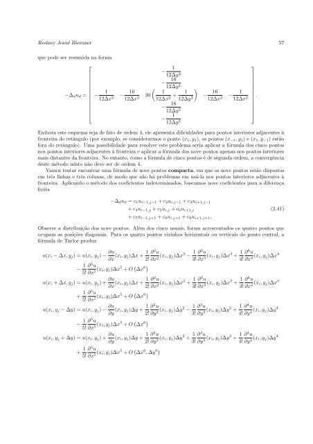
Rodney Josué Biezuner 57
que pode ser resumida na forma
⎡
⎢
−∆dud = ⎢
⎣
− 1 16
−
12∆x2 12∆x2 − 1
12∆y2 − 16
12∆y2
1 1
30 +
12∆x2 12∆y2
− 16
12∆y2 − 1
12∆y2 − 16 1
−
12∆x2 12∆x2 Embora este esquema seja de fato de ordem 4, ele apresenta dificuldades para pontos interiores adjacentes à
fronteira do retângulo (por exemplo, se considerarmos o ponto (x1, y1), os pontos (x−1, y1) e (x1, y−1) estão
fora do retângulo). Uma possibilidade para resolver este problema seria aplicar a fórmula dos cinco pontos
nos pontos interiores adjacentes à fronteira e aplicar a fórmula dos nove pontos apenas nos pontos interiores
mais distantes da fronteira. No entanto, como a fórmula de cinco pontos é de segunda ordem, a convergência
deste método misto não deve ser de ordem 4.
Vamos tentar encontrar uma fórmula de nove pontos compacta, em que os nove pontos estão dispostos
em três linhas e três colunas, de modo que não há problemas em usá-la nos pontos interiores adjacentes à
fronteira. Aplicando o método dos coeficientes indeterminados, buscamos nove coeficientes para a diferença
finita
−∆dud = c1ui−1,j−1 + c2ui,j−1 + c3ui+1,j−1
+ c4ui−1,j + c5ui,j + c6ui+1,j
+ c7ui−1,j+1 + c8ui,j+1 + c9ui+1,j+1.
⎤
⎥ .
⎥
⎦
(2.41)
Observe a distribuição dos nove pontos. Além dos cinco usuais, foram acrescentados os quatro pontos que
ocupam as posições diagonais. Para os quatro pontos vizinhos horizontais ou verticais do ponto central, a
fórmula de Taylor produz
u(xi − ∆x, yj) = u(xi, yj) − ∂u
∂x (xi, yj)∆x + 1
2!
− 1 ∂
5!
5u ∂x5 (xi, yj)∆x 5 + O ∆x 6
u(xi + ∆x, yj) = u(xi, yj) + ∂u
∂x (xi, yj)∆x + 1
2!
+ 1 ∂
5!
5u ∂x5 (xi, yj)∆x 5 + O ∆x 6
u(xi, yj − ∆y) = u(xi, yj) − ∂u
∂y (xi, yj)∆y + 1
2!
− 1 ∂
5!
5u ∂x5 (xi, yj)∆x 5 + O ∆x 6
u(xi, yj + ∆y) = u(xi, yj) + ∂u
∂y (xi, yj)∆y + 1
2!
+ 1 ∂
5!
5u ∂x5 (xi, yj)∆x 5 + O ∆x 6 , ∆y 6
∂2u ∂x2 (xi, yj)∆x 2 − 1 ∂
3!
3u ∂x3 (xi, yj)∆x 3 + 1 ∂
4!
4u ∂x4 (xi, yj)∆x 4
∂2u ∂x2 (xi, yj)∆x 2 + 1 ∂
3!
3u ∂x3 (xi, yj)∆x 3 + 1 ∂
4!
4u ∂x4 (xi, yj)∆x 4
∂2u ∂y2 (xi, yj)∆y 2 − 1 ∂
3!
3u ∂y3 (xi, yj)∆y 3 + 1 ∂
4!
4u ∂y4 (xi, yj)∆y 4
∂2u ∂y2 (xi, yj)∆y 2 + 1 ∂
3!
3u ∂y3 (xi, yj)∆y 3 + 1 ∂
4!
4u ∂y4 (xi, yj)∆y 4