Tese em PDF - departamento de engenharia florestal ...

More documents

Recommendations

Info

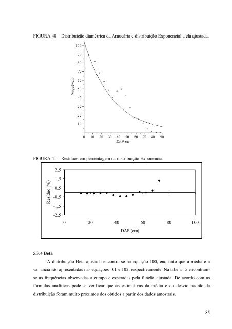
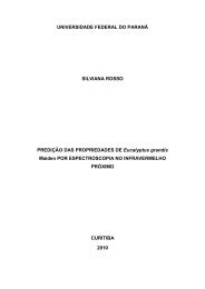
f ( x) −x ⎧ 1 , 77 ⎪ ⋅ e para x ≥ 0, = ⎨32, 77 ⎪ ⎩0 e.o.c. 32 β > 0 EQ. 97 μ = 32, 77 cm EQ. 98 = 2 2 σ X 1073, 72 cm EQ. 99 TABELA 14 – Distribuição diamétrica, frequências acumuladas esperadas pela distribuição Exponencial ajustada e diferença absoluta entre as distribuições acumuladas esperada e observada. Li|-ls Xi fobs Fobs Fesp |Fesp-Fobs| 10|-15 12,5 82 82 165,87 83,87 15|-20 17,5 69 151 216,41 65,41 20|-25 22,5 59 210 259,80 49,80 25|-30 27,5 49 259 297,04 38,04 30|-35 32,5 41 300 329,02 29,02 35|-40 37,5 48 348 356,47 8,47 40|-45 42,5 50 398 380,04 17,96 45|-50 47,5 43 441 400,27 40,73 50|-55 52,5 29 470 417,64 52,36 55|-60 57,5 17 487 432,55 54,45 60|-65 62,5 16 503 445,35 57,65 65|-70 67,5 11 514 456,34 57,66 70|-75 72,5 5 519 465,77 53,23 75|-80 77,5 2 521 473,87 47,13 80|-85 82,5 1 522 480,82 41,18 > 85 87,5 1 523 486,79 36,21 Total 523 Comparando a razão da máxima diferença entre as frequências acumulas observada e estimada pela distribuição Exponencial (KS = 0,1604) com os valores tabelados, observa-se que ela não foi aderente, como já se esperava, uma vez que essa distribuição não apresenta modas. Este modelo tem sido testado e utilizado amplamente em função de sua simplicidade de ajuste e bons resultados em muitos casos de florestas naturais, contudo, na distribuição que está sendo utilizada, não gerou um resultado satisfatório. Encontra-se na figura 40 o gráfico dos valores observados, bem como a curva ajustada. Com o auxílio dessa imagem é possível ratificar que a distribuição não é capaz de representar de forma satisfatória a distribuição diamétrica da Araucária. Outro bom indicador encontra-se na figura 41, onde estão apresentados os resíduos percentuais entre valores estimados pelo modelo e observados a campo. 84
FIGURA 40 – Distribuição diamétrica da Araucária e distribuição Exponencial a ela ajustada. FIGURA 41 – Resíduos em percentagem da distribuição Exponencial Resíduo (%) 5.3.4 Beta 2,5 1,5 0,5 -0,5 -1,5 -2,5 0 20 40 60 80 100 DAP (cm) A distribuição Beta ajustada encontra-se na equação 100, enquanto que a média e a variância são apresentadas nas equações 101 e 102, respectivamente. Na tabela 15 encontram- se as frequências observadas a campo e esperadas pela função ajustada. De acordo com as fórmulas analíticas pode-se verificar que as estimativas da média e do desvio padrão da distribuição foram muito próximos dos obtidos a partir dos dados amostrais. 85
Page 1 and 2:
SAULO HENRIQUE WEBER Desenvolviment
Page 3 and 4:
DEDICATÓRIA Dedico esse trabalho
Page 5 and 6:
e processuais dentro da instituiç
Page 7 and 8:
SUMÁRIO 1. INTRODUÇÃO...........
Page 9 and 10:
5.2.3 Exponencial .................
Page 11 and 12:
FIGURA 24 - Resíduos em percentage
Page 13 and 14:
LISTA DE TABELAS TABELA 01 - Dados
Page 15 and 16:
RESUMO A tendência da distribuiç
Page 17 and 18:
1. INTRODUÇÃO A palavra, hoje amp
Page 19 and 20:
cálculos eram realizados sem o aux
Page 21 and 22:
1.2 OBJETIVOS 1.2.1 Objetivo Geral
Page 23 and 24:
e tal que para qualquer sucesso de
Page 25 and 26:
• Se f é contínua em ( ∞, a]
Page 27 and 28:
uma floresta, é mais fácil explor
Page 29 and 30:
FIGURA 01 - Representação da áre
Page 31 and 32:
A distribuição probabilística bi
Page 33 and 34:
O melhor ajuste foi obtido com a ds
Page 35 and 36:
Mesquita et al. (2007) testaram uma
Page 37 and 38:
exponencial tem sido utilizada para
Page 39 and 40:
FIGURA 03 - REPRESENTAÇÃO GRÁFIC
Page 41 and 42:
FIGURA 05 - REPRESENTAÇÃO GRÁFIC
Page 43 and 44:
f ( x) ⎧ c c ⎪ ⎛ x − a ⎞
Page 45 and 46:
1. A curva normal tem forma de sino
Page 47 and 48:
2.5.7 Funções Spline Em uma Funç
Page 49 and 50: Outro fator que contribui para a oc
Page 51 and 52: 3. MATERIAIS E MÉTODOS Para o dese
Page 53 and 54: ( ) = ( −1)! Γ α α EQ. 27 Γ
Page 55 and 56: 3.6 DISTRIBUIÇÃO WEIBULL f ( x) A
Page 57 and 58: 1 7. Multiplicar a função por , a
Page 59 and 60: d calc ( F ( X ) − F ( X ) ) = ma
Page 61 and 62: Curva Normal tem um desempenho aqu
Page 63 and 64: Além disso, verifica-se a existên
Page 65 and 66: FIGURA 12 - Resultado do terceiro t
Page 67 and 68: 4.4.6 Teste 6 Ao se adicionar o pro
Page 69 and 70: 4.4.9 Teste 9 Um resultado satisfat
Page 71 and 72: ( ) ( ) ( ) ( ) ( ) 2 2 2 x 0. 5339
Page 73 and 74: 5.1 INTRODUÇÃO 5. RESULTADOS E DI
Page 75 and 76: etc. A única também onde foram co
Page 77 and 78: TABELA 03 - Distribuição diamétr
Page 79 and 80: f ( x) −x ⎧ 1 , 26 ⎪ ⋅ e pa
Page 81 and 82: 0, 27 ( x −10) ⋅ ( 190 − x) 0
Page 83 and 84: f ⎧ ⎪ ( x) = 4, 45 ⎨20, 51
Page 85 and 86: f ( x) ⎧ ⎪ ⎛ x −14, 95 0, 0
Page 87 and 88: verificado que retirando-se apenas
Page 89 and 90: 5.2.8 Spline Cúbica A Função Spl
Page 91 and 92: FIGURA 33 - Distribuição diamétr
Page 93 and 94: FDP = EQ. 93 1 16. 055, 87 ⋅ 1, 1
Page 95 and 96: TABELA 11 - Comparação entre os m
Page 97 and 98: FIGURA 37 - Estrutura populacional
Page 99: FIGURA 38 - Distribuição diamétr
Page 109 and 110: apresentados os resíduos percentua
Page 111 and 112: TABELA 19 - Distribuição diamétr
Page 113 and 114: Os coeficientes b e d são dependen
Page 115 and 116: de 56.863,56 cm², ou seja, desvio
Page 117 and 118: 5.4 Araucaria angustifolia Criada e
Page 119 and 120: será feita a comparação entre os
Page 121 and 122: média estimada pela distribuição
Page 123 and 124: −0, 1196 ( x −10) ⋅ ( 90 −
Page 125 and 126: f ⎧ ⎪ ( x) = 4, 33 ⎨10, 03
Page 127 and 128: A média e a variância estão apre
Page 129 and 130: a flexibilidade apresentada pelo mo
Page 131 and 132: 5.4.8 Spline Cúbica A Função Spl
Page 133 and 134: FIGURA 68 - Resíduos em percentage
Page 137 and 138: TABELA 31 - Comparação entre os m
Page 139 and 140: O modelo apresentado por Silva et a
Page 141 and 142: origem. O que muda de um caso para
Page 143 and 144: DUCKE, A.; G. A.; BLACK. G. A. Nota
Page 145 and 146: MACHADO, S. A.; SIQUEIRA, J. D. P.
Page 147 and 148: SANTOS, A. S. A. Modelos simétrico
show all

Tese em PDF - departamento de engenharia florestal ...

Create successful ePaper yourself

Delete template?

Save as template?