现代统计图形 - 科学网—博客

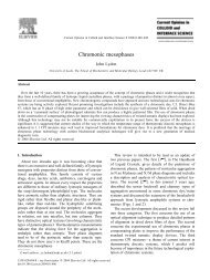
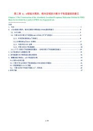
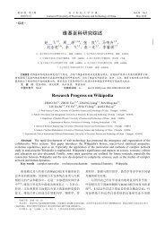
78 第五章 图库
1 > # 原始数据:是否失效以及相应温度
2 > fail = factor(c(2, 2, 2, 2, 1, 1, 1, 1, 1, 1, 2,
3 + 1, 2, 1, 1, 1, 1, 2, 1, 1, 1, 1, 1), levels = 1:2,
4 + labels = c("no", "yes"))
5 > temperature = c(53, 57, 58, 63, 66, 67, 67, 67, 68,
6 + 69, 70, 70, 70, 70, 72, 73, 75, 75, 76, 76, 78,
7 + 79, 81)
8 > par(mar = c(4, 4, 0.5, 2))
9 > cdplot(fail ~ temperature, col = c("lightblue", "red"))
10 > # 用黄色的点表示原始数据;注意y轴位置不是c(1, 2)!
11 > # 请思考为什么(看源代码 getS3method(cdplot, default))
12 > points(temperature, c(0.25, 0.75)[as.integer(fail)],
13 + col = "blue", bg = "yellow", pch = 21)
fail
no yes
55 60 65 70 75 80
temperature
图 5.10: 航天飞机O型环在不同温度下失效的条件密度图:随着温度升高,
O型环越来越不容易失效。
0.0 0.2 0.4 0.6 0.8 1.0