现代统计图形 - 科学网—博客

More documents

Recommendations

Info

82 第五章图库 1 > par(mar = rep(0, 4)) 2 > # 继续前面的例子 3 > persp(est[["x1"]], est[["x2"]], est[["fhat"]], shade = 0.75, 4 + border = NA, col = "lightblue", phi = 20, theta = 15, 5 + box = FALSE) 图 5.13: 与等高图对应的三维透视图:本图与图5.12对应,从右至左依次有三个山峰,尤其是中部的山峰最为突出,对照后面5.26小节中图5.34可知, 这三个山峰分别代表了东中西的省份。
5.8 等高图 83 都必须展示在静态介质上(如书籍、论文等),我们不可能在纸面上拖动鼠标对图形进行交互式操作,因此,我们需要等高图这样一种以二维形式展示三维数据的工具。首先我们需要理解等高图所展示数据的形式,因为它与我们想象的三维数据有所不同:并非三个数值向量,而是两个数值向量x、y和一个相应的矩阵z。我们不妨将数据的形式想象为一座山峰,两个数值向量分别是横向和纵向的位置(如经纬度),第三维数据是每一种横纵向位置点组合上的高度,而横纵交叉组合之后形成的是一个“网格”,矩阵z则是这个网格上的高度数值,用数学式子表示这种关系就是zij = f(xi, yj)。图5.11为这种网格数据的示意图,请读者自行体会。所谓等“高”线,就是将平面上对应的z值(高度)相等的点连接起来形成的线。同样,我们可以以一座山峰来想象:在同一海拔高度上围绕山峰一圈的线就是一条等高线。图5.11中的连线即等高线,如实线表示的是高度为2的点,而虚线表示高度为1的点。注意等高线之间不可能相交,因为同一点不可能同时有两种高度。等高线上通常会有数字表示高度,从这些数字我们不难想象出三维的 “山峰”的形状,从这个意义上来说,等高图本质上也是一种三维图示方法。 R中等高图的函数为contour(),同时grDevices包中也提供了等高线的计算函数contourLines(),用法分别如下: 1 > usage(contour, "default") contour(x = seq(0, 1, length.out = nrow(z)), y = seq(0, 1, length.out = ncol(z)), z, nlevels = 10, levels = pretty(zlim, nlevels), labels = NULL, xlim = range(x, finite = TRUE), ylim = range(y, finite = TRUE), zlim = range(z, finite = TRUE), labcex = 0.6, drawlabels = TRUE, method = "flattest", vfont, axes = TRUE, frame.plot = axes, col = par("fg"), lty = par("lty"), lwd = par("lwd"), add = FALSE, ...) 1 > usage(contourLines) contourLines(x = seq(0, 1, length.out = nrow(z)), y = seq(0, 1, length.out = ncol(z)), z, nlevels = 10, levels = pretty(range(z, na.rm = TRUE), nlevels))
Page 1 and 2:
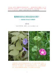
现代统计图形谢益辉 2010
Page 3 and 4:
• 自由软件用户往往有某
Page 5 and 6:
目录序言 i 代序一 . . . . .
Page 7 and 8:
5.25 向日葵散点图 . . . . . .
Page 9:
附录 B 作图技巧 163 B.1 添
Page 12 and 13:
5.4 泊松分布随机数茎叶图
Page 15 and 16:
表格 5.1 二维列联表的经典
Page 17 and 18:
序言代序一代序二作者
Page 19:
Coefficients: Estimate Std. Error t
Page 22 and 23:
2 第一章历史图 1.1: Playfai
Page 24 and 25:
4 第一章历史吸到了“瘴
Page 26 and 27:
6 第一章历史图 1.4: 南丁
Page 28 and 29:
8 第一章历史图 1.5: Minard
Page 30 and 31:
10 第一章历史总的说来,
Page 32 and 33:
12 第二章工具大小,如条
Page 34 and 35:
14 第二章工具 Type contributo
Page 36 and 37:
16 第二章工具百K的一个
Page 38 and 39:
18 第二章工具其实没有必
Page 40 and 41:
20 第二章工具
Page 42 and 43:
22 第三章细节 3.1 par()函数
Page 44 and 45:
24 第三章细节 1:10 2 4 6 8 10
Page 46 and 47:
26 第三章细节 las 坐标轴
Page 48 and 49:
28 第三章细节 oma[2] mar[2] O
Page 50 and 51:
30 第三章细节 3.2 plot()及
Page 52 and 53: 32 第三章细节 xlim, ylim 设
Page 54 and 55: 34 第四章元素 4.1 颜色默
Page 56 and 57: 36 第四章元素 4.1.2 颜色生
Page 58 and 59: 38 第四章元素 [,1] [,2] [,3]
Page 60 and 61: 40 第四章元素每一类调色
Page 62 and 63: 42 第四章元素 1 > xx = c(1912
Page 64 and 65: 44 第四章元素 0 1 2 3 4 5 6 7
Page 66 and 67: 46 第四章元素图2.1已经使
Page 68 and 69: 48 第四章元素 1 > usage(arrow
Page 70 and 71: 50 第四章元素一个多边形
Page 72 and 73: 52 第四章元素可以看到,
Page 74 and 75: 54 第四章元素 1 > par(mar = c
Page 76 and 77: 56 第四章元素 1 > data(Export
Page 78 and 79: 58 第四章元素 12 72.48 2003 U
Page 80 and 81: 60 第五章图库 1 > par(mfrow =
Page 82 and 83: 62 第五章图库 f(x) = F ′ F
Page 84 and 85: 64 第五章图库 1 > stem(island
Page 86 and 87: 66 第五章图库对原始数据
Page 88 and 89: 68 第五章图库 names, plot = T
Page 90 and 91: 70 第五章图库 1 > par(mar = c
Page 92 and 93: 72 第五章图库 1 > # 用分类
Page 94: 74 第五章图库 1 > library(MSG
Page 97 and 98: 5.7 条件密度图 77 R中关联
Page 99 and 100: 5.7 条件密度图 79 小到大在
Page 101: 5.8 等高图 81 1 > data(ChinaLife
Page 105 and 106: 5.9 条件分割图 85 1 > par(mar
Page 107 and 108: 5.10 一元函数曲线图 87 1 > c
Page 109 and 110: 5.12 颜色等高图 89 1 > dotchar
Page 111 and 112: 5.13 四瓣图 91 finite = TRUE), y
Page 113 and 114: 5.13 四瓣图 93 表 5.1: 二维
Page 115 and 116: 5.14 颜色图 95 C和E系的优比
Page 117 and 118: 5.14 颜色图 97 1 > par(mar = rep
Page 119 and 120: 5.15 矩阵图 99 1 > sines = outer
Page 121 and 122: 5.16 马赛克图 101 1 > ftable(Ti
Page 123 and 124: 5.17 散点图矩阵 103 较低。
Page 125 and 126: 5.18 三维透视图 105 倍数;fon
Page 127 and 128: 5.18 三维透视图 107 Sinc( r )
Page 129 and 130: 5.19 因素效应图 109 1 > plot.d
Page 131 and 132: 5.21 平滑散点图 111 1 > par(ma
Page 133 and 134: 5.22 棘状图 113 可将图5.28放
Page 135 and 136: 5.22 棘状图 115 离散化处理,
Page 137 and 138: 5.23 星状图 117 1 > # 预设调
Page 139 and 140: 5.24 带状图 119 1 > layout(matri
Page 141 and 142: 5.25 向日葵散点图 121 1 > sun
Page 143 and 144: 5.26 符号图 123 1 > par(mar = c(
Page 145: 5.27 饼图 125 增长率总人口
Page 148 and 149: 128 第五章图库种以比例
Page 150 and 151: 130 第五章图库 1 > # 真实
Page 152 and 153:
132 第五章图库信用风险
Page 154 and 155:
134 第五章图库 1 > library(rp
Page 156 and 157:
136 第五章图库有时候与
Page 158 and 159:
138 第五章图库数诸如填
Page 160 and 161:
140 第五章图库
Page 162 and 163:
142 第六章系统 8 > plot(0:1,
Page 164 and 165:
144 第七章模型 • 类似回
Page 166 and 167:
146 第七章模型 7.16.1 分类
Page 168 and 169:
148 第八章数据 8.2.1 一维
Page 170 and 171:
150 附录 A 程序初步通常我
Page 172 and 173:
152 附录 A 程序初步 1 > # 冒
Page 174 and 175:
154 附录 A 程序初步 [1] 1 2 3
Page 176 and 177:
156 附录 A 程序初步 [,1] [,2]
Page 178 and 179:
158 附录 A 程序初步 A.1.5 函
Page 180 and 181:
160 附录 A 程序初步 [1] "inte
Page 182 and 183:
162 附录 A 程序初步 2. 变量
Page 184 and 185:
164 附录 B 作图技巧 1 > # 本
Page 186 and 187:
166 附录 B 作图技巧 1 > layou
Page 188 and 189:
168 附录 B 作图技巧 screen(n
Page 190 and 191:
170 附录 B 作图技巧 B.3 交
Page 192 and 193:
172 附录 B 作图技巧 1 > xx =
Page 194 and 195:
174 附录 B 作图技巧正的频
Page 196 and 197:
176 附录 B 作图技巧
Page 198 and 199:
178 附录 C 统计动画
Page 200 and 201:
180 附录 D 本书R包 D.2 数据
Page 202 and 203:
182 参考文献 Minka , URL http:/
Page 204 and 205:
184 参考文献 Meyer D, Zeileis A
Page 206 and 207:
186 参考文献 Wilkinson L (2005)
Page 208 and 209:
188 索引点, 27 玫瑰图, 4 直
Page 210:
190 索引形的一些历史,包
show all

现代统计图形 - 科学网—博客

Create successful ePaper yourself

Delete template?

Save as template?