Regressione Multipla_03 - Dipartimento di Economia e Statistica

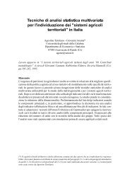
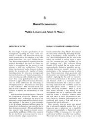
Cause della eteroschedasticità!Le unità campionarie provengono da sottopopolazioni diverseovvero da aree diverse.!Ad esempio, nelle imprese di minori dimensioni la variabilità delle venditeè più contenuta che in quelle maggiori che tendono ad essere più volatili. !Nel campione sono più presenti unità con maggiore o minorevariabilità rispetto alle altre!Ad esempio, le unità rilevate al centro-città potrebbero essere poche sequelle in periferia sono più numerose per includere nel campione tutte leperiferie!Uno o più regressori importanti sono stati omessi ovvero noncompaiono nella forma più adatta.!Talvolta inserire Log(x) oppure #x invece di x può eliminare la eteroschedasticità.!La mancanza di un regressore importante non è un problema dieteroschedasticità, ma di corretta specificazione del modello!Dove si incontra!E# comune nei data set in cui si riscontra una forte escursione neivalori: sono presenti valori molto piccoli e molto grandi !E# anche presente nei dati cross-section in cui si aggregano daticon diversa natura e quindi potenzialmente diversa variabilità !Nelle serie storiche con un forte trend monotono si riscontraspesso una diversa struttura di variabilità tra la fase iniziale equella finale del fenomeno !Non è infrequente trovarla nelle indagini campionarie in cui lafase di acquisizione si modifica in aspetti rilevanti.!Errori eteroschedastici/2!Per migliorare l#aderenza ai fenomeni reali ipotizziamo errori incorrelati,ma eteroschedastici!# 10 0&0 #( ) = " 2 & 20E uu t$')&) = " 2 *)&% 0 0)# n (In cui la variabilità non è costante, ma cambia anche se non necessariamente! le varianze sono tutte diverse.!E# possibile infatti immaginare gruppi di osservazioni con varianzaomogenea, che è però diversa nei vari gruppi!Stima dei parametri!Se V è una matrice simmetrica e definita positiva possiamo scrivere!Dove !Q è la matrice formata con gli autovettori di norma unitaria associati agliautovalori di V;!# 0.5 è la!matrice diagonale i cui elementi non nulli sono le radici degliautovalori di V.!Se la matrice V è diagonale gli autovalori coincidono con i suoi elementinon nulli e gli autovettori sono i vettori identità (cioè Q=I). !Quindi!V = ( Q" 0.5)( Q" 0.5) t˜ " = [ X t # $0.5 # $0.5 X] $1 X t # $0.5 # $0.5 y % ˜ " = [ W t W ] $1 W t zIn questo caso la matrice " è diagonale formata da elementi positivi,non necessariamente tutti distinti.!!Dove ora W=X # -0.5 e z=y # -0.5 .!

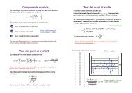
Stima dei parametri/2!Conseguenze sugli stimatori!Lo stimatore ai minimiquadrati in presenza dierrori eteroschedastici è lostimatore OLS, maapplicato a variabili pesate!# y 1&% ("% 1(% y 2 (z = % " 2(; W =% … (% yn(% ($ " n '#%%%%%%%$ %1 x 11x 12… x &1m" 1" 1" 1"(11 x 21x 22… x (2m (" 2" 2" 2" 2(… … … … ((1" nx n1" nx n 2" n… x nm" n('(Nulla cambia rispetto alla caratteristica di stimatore BLUE (se " è nota)!La bontà di adattamento in termini di R 2 non risente del cambiamento!R 2 = Dev.Spieg. = y t CHyDev.Tot. y t Cy = SSRSST!Ovvero un modello di regressione lineare multipla così formulato!!y $i1= # 0"&i %" i') + # $ x 'i11&( % ") + # $2&i ( %x i2" i') +…+ # $ xim'2&( % ") + u ii (L"i-esimo dato (y i ,x i1 , x i2 … x im ) è pesato con il reciproco della radicedell"autovalore " i : i casi con maggiore variabilità pesano meno laddovesono più rilevanti le osservazioni con minore dispersione!Conseguenze sugli stimatori/2!Che succede se si stimano i parametri come se " = I , ma in realtà" " I ? !Gli stimatori rimangono non distorti.!" iL#impatto della divisione per i pesi $ i si annulla.!!La varianza degli stimatori dipende dai pesi $ i !!Var( ˜ ") = [ X t # $1 X] $1Operatività della tecnica!La eteroschedasticità è un fenomeno che riguarda la potenzialità di erroreper le singole osservazioni che si modifica al modificarsi delle osservazioni.!Non avrebbe alcuna conseguenza se la matrice di varianze-covarianze fossenota ovvero incognita nel solo parametro ! 2 .!Ovviamente non son più gli stimatori BLUE del modello, ma anzihanno una variabilità che può essere molto superiore o moltoinferiore.!In pratica si opera con due livelli di ignoranza!Le diagnostiche basate sui t-Student, sull#F-Fisher e sull#R 2 sonopiù alte (o più basse) di quanto non dovrebbero!Non sappiamo se gli errori sono omo- oppure etero-schedastici!C#è il rischio di giudicare buono o cattivo un modello che lo èsolo in virtù di una falsa premessa sulla omoshcedasticità!Nel secondo caso non sappiamo quanti e quali siano i pesi $ i chedebbono quindi essere stimati.!I parametri da stimare sono m+n (m in ! ed n in #) quindi più parametriche dati. Come se ne esce?!

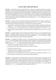
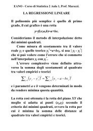
Test di Park/2!La difficoltà maggiore con questo test è la scelta dei valori della z i .!Su questo possiamo dare solo indicazioni!Dovrebbe essere un FATTORE DIMENSIONALE ovvero i quadrati degli erroridovrebbero variare con i valori di questa variabile.!La relazione tra errori e fattore dimensionale dovrebbe essere almenomonotona.!La disponibilità del fattore dimensionale potrebbe tornare utile per eliminareo ridurre il problema della eteroschedasticità.!y X1 X224.0 2 7.827.4 4 9.821.8 8 1.217.6 6 0.224.9 5 6.529.1 7 6.825.2 3 7.927.9 9 2.724.2 6 6.017.5 1 4.324.5 3 7.017.5 1 4.336.1 9 9.822.8 7 2.928.5 8 5.423.7 6 2.633.1 9 9.328.9 4 9.439.6 2 26.565.9 9 28.330.6 6 13.622.3 1 13.137.0 3 22.328.7 5 14.225.7 3 13.338.2 1 27.440.4 8 19.344.7 6 15.133.2 5 18.137.6 3 14.939.3 1 18.247.6 9 15.147.1 4 19.640.6 2!28.036.4 1 16.947.2 6 17.8Residuals1086420-2-4-6-81020p " value per # 1in Ln e i2p " value per # 1in Ln e i230Esempio!Predicted vs. Residual ScoresPredicted Values( ) = # 0+ # 1Ln( x i1 ) : 0.1041( ) = # 0+ # 1Ln( x i2 ) : 0.0035C#è una fortissima evidenza di eteroschedasticità,almeno in relazione al 2° regressore!40506070Esercizio!GDP LFG EQP NEQ GAP 0.0149 0.0242 0.0384 0.0516 0.7885 -0.0047 0.0283 0.0358 0.0842 0.85790.0089 0.0118 0.0214 0.2286 0.6079 0.0148 0.0303 0.0446 0.0954 0.8850 0.0260 0.0150 0.0701 0.2199 0.37550.0332 0.0014 0.0991 0.1349 0.5809 0.0484 0.0359 0.0767 0.1233 0.7471 0.0295 0.0258 0.0263 0.0880 0.91800.0256 0.0061 0.0684 0.1653 0.4109 0.0115 0.0170 0.0278 0.1448 0.9356 0.0295 0.0279 0.0388 0.2212 0.80150.0124 0.0209 0.0167 0.1133 0.8634 0.0345 0.0213 0.0221 0.1179 0.9243 0.0261 0.0299 0.0189 0.1011 0.84580.0676 0.0239 0.1310 0.1490 0.9474 0.0288 0.0081 0.0814 0.1879 0.6457 0.0107 0.0271 0.0267 0.0933 0.74060.0437 0.0306 0.0646 0.1588 0.8498 0.0452 0.0305 0.1112 0.1788 0.6816 0.0179 0.0253 0.0445 0.0974 0.87470.0458 0.0169 0.0415 0.0885 0.9333 0.0362 0.0038 0.0683 0.1790 0.5441 0.0318 0.0118 0.0729 0.1571 0.80330.0169 0.0261 0.0771 0.1529 0.1783 0.0278 0.0274 0.0243 0.0957 0.9207 -0.0011 0.0274 0.0193 0.0807 0.88840.0021 0.0216 0.0154 0.2846 0.5402 0.0055 0.0201 0.0609 0.1455 0.8229 0.0373 0.0069 0.0397 0.1305 0.66130.0239 0.0266 0.0229 0.1553 0.7695 0.0535 0.0117 0.1223 0.2464 0.7484 0.0137 0.0207 0.0138 0.1352 0.85550.0121 0.0354 0.0433 0.1067 0.7043 0.0146 0.0346 0.0462 0.1268 0.9415 0.0184 0.0276 0.0860 0.0940 0.97620.0187 0.0115 0.0688 0.1834 0.4079 0.0479 0.0282 0.0557 0.1842 0.8807 0.0341 0.0278 0.0395 0.1412 0.91740.0199 0.0280 0.0321 0.1379 0.8293 0.0236 0.0064 0.0711 0.1944 0.2863 0.0279 0.0256 0.0428 0.0972 0.78380.0283 0.0274 0.0303 0.2097 0.8205 -0.0102 0.0203 0.0219 0.0481 0.9217 0.0189 0.0048 0.0694 0.1132 0.43070.0046 0.0316 0.0223 0.0577 0.8414 0.0153 0.0226 0.0361 0.0935 0.9628 0.0133 0.0189 0.0762 0.1356 0.00000.0094 0.0206 0.0212 0.0288 0.9805 0.0332 0.0316 0.0446 0.1878 0.7853 0.0041 0.0052 0.0155 0.1154 0.57820.0301 0.0083 0.1206 0.2494 0.5589 0.0044 0.0184 0.0433 0.0267 0.9478 0.0120 0.0378 0.0340 0.0760 0.49740.0292 0.0089 0.0879 0.1767 0.4708 0.0198 0.0349 0.0273 0.1687 0.5921 -0.0110 0.0275 0.0702 0.2012 0.86950.0259 0.0047 0.0890 0.1885 0.4585 0.0243 0.0281 0.0260 0.0540 0.8405 0.0110 0.0309 0.0843 0.1257 0.88750.0446 0.0044 0.0655 0.2245 0.7924 0.0231 0.0146 0.0778 0.1781 0.3605Rimedi: minimi quadrati generalizzati!Se i grafici ed i test concordano nel segnalare la presenza di una variabilitànon omogenea nei dati occorre ridurre il problema.!Se si è usato il test di Park e si è accertato che c#è eteroschedasticità dovutaal regressore x k cioè si pensa Var(u i )=! 2 (X ik ) 2 , si può agire sul modello!y $i1 ' $ x ' $= " 0+ # 0 & ) + # i1x '$1 & ) + # i2x '2 & ) +…+ # k+…+ # m & im) + u ix ik % x ik ( % x ik ( % x ik (% x ik ( x ikz i= # k+ # 0w i0+ # 1w i1+ # 2w i2+…+ # mw im+ v iDe Long and Summers (1991) studied the national growth of61 countries from 1960 to 1985 using OLS. The regressionequation they used is !GDP = & 0 + & 1 LFG+ & 2 GAP + & 3 EQP + & 4 NEQ+u !where !GDP growth per worker LFG labor force growth !GAP relative GDP gap EQP equipment investment!NEP non- equipment investment . !Stimare il modello diregressione e verificare lapresenza di eteroschedasticità!!il coefficiente del primo regressore del nuovo modello è l"intercetta delmodello originario. !L"intercetta del nuovo modello è il coefficiente angolare del fattore diproporzionalità nel vecchio modello.!

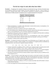
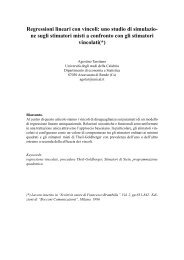
y X0 X1 X2 Z W1 W2 W024.0 1.0 2 7.8 3.07 0.13 0.72 0.3627.4 1.0 4 9.8 2.79 0.10 0.41 1.0021.8 1.0 8 1.2 18.20 0.83 6.67 1.0017.6 1.0 6 0.2 88.20 5.00 30.00 1.0024.9 1.0 5 6.5 3.83 0.15 0.77 1.0029.1 1.0 7 6.8 4.27 0.15 1.03 1.0025.2 1.0 3 7.9 3.19 0.13 0.38 1.0027.9 1.0 9 2.7 10.35 0.37 3.33 1.0024.2 1.0 6 6.0 4.03 0.17 1.00 1.0017.5 1.0 1 4.3 4.06 0.23 0.23 1.0024.5 1.0 3 7.0 3.50 0.14 0.43 1.0017.5 1.0 1 4.3 4.06 0.23 0.23 1.0036.1 1.0 9 9.8 3.68 0.10 0.92 1.0022.8 1.0 7 2.9 7.86 0.34 2.41 1.0028.5 1.0 8 5.4 5.27 0.19 1.48 1.00 !23.7 1.0 6 2.6 9.12 0.38 2.31 1.0033.1 1.0 9 9.3 3.55 0.11 0.97 1.0028.9 1.0 4 9.4 3.07 0.11 0.43 1.0039.6 1.0 2 26.5 1.49 0.04 0.08 1.0065.9 1.0 9 28.3 2.33 0.04 0.32 1.0030.6 1.0 6 13.6 2.25 0.07 0.44 1.0022.3 1.0 1 13.1 1.70 0.08 0.08 1.0037.0 1.0 3 22.3 1.66 0.04 0.13 1.0028.7 1.0 5 14.2 2.02 0.07 0.35 1.0025.7 1.0 3 13.3 1.93 0.08 0.23 1.0038.2 1.0 1 27.4 1.39 0.04 0.04 1.0040.4 1.0 8 19.3 2.09 0.05 0.41 1.0044.7 1.0 6 15.1 2.96 0.07 0.40 1.0033.2 1.0 5 18.1 1.84 0.06 0.28 1.0037.6 1.0 3 14.9 2.52 0.07 0.20 1.0039.3 1.0 1 18.2 2.16 0.05 0.05!1.0047.6 1.0 9 15.1 3.15 0.07 0.60 1.0047.1 1.0 4 19.6 2.40 0.05 0.20 1.0040.6 1.0 2 28.0 1.45 0.04 0.07 1.0036.4 1.0 1 16.9 2.15 0.06 0.06 1.0047.2 1.0 6 17.8 2.65 0.06 0.34 1.00Continua esempio!Test di White per la regressione di zsu w 1 e w 2 !F h= 0.021 # 33&% ( = 0.35 ) p " value = 0.711" 0.021$2 'L#eteroschedasticità è stata rimossa!Var v i( ) = Var"$#u ix ik%' = 1& x Var u 2 iik= 1x ik2 ( 2 x ik 2 = ( 2( )per ogni iQuesta procedura crea delle perplessità. !Che ruolo ha il regressore che opera comefattore di proporzionalità?!Agisce in proprio o subisce l"effetto di unfattore esterno comune alla dipendente?!Rimedi: uso dei valori stimati!Se nessuno dei regressori appare collegato alla eteroschedasticità !Ovvero non riusciamo a determinare il tipo di legame che unisce uno o piùregressori agli errori!possiamo ipotizzare che!E quindi agire sul modello!Var( u i ) = " 2 y ˆ i!y i# 1 & # x= "y ˆ 0 % ( + " i1& # xi $ ˆ 1 % ( + " i2& # x' $ ˆ 2 % ( +…+ " im&' $ ˆm % ( + u i' $ ˆ ' ˆy iIn questo caso il modello è da stimare senza intercetta.!y iz i= " 0w i0+ " 1w i1+ " 2w i2+…+ " mw im+ v iy iy iy i!y X0 X1 X2 Z W1 W224.0 1.0 2 7.8 11.09 0.93 3.6127.4 1.0 4 9.8 -92.65 -13.55 -33.1921.8 1.0 8 1.2 -8.69 -3.18 -0.4817.6 1.0 6 0.2 -8.61 -2.93 -0.1024.9 1.0 5 6.5 -44.54 -8.94 -11.6329.1 1.0 7 6.8 -126.99 -30.59 -29.7225.2 1.0 3 7.9 16.51 1.97 5.1827.9 1.0 9 2.7 433.04 139.49 41.8524.2 1.0 6 6.0 -10.09 -2.50 -2.5017.5 1.0 1 4.3 11.14 0.64 2.7424.5 1.0 3 7.0 12.78 1.56 3.6517.5 1.0 1 4.3 11.14 0.64 2.7436.1 1.0 9 9.8 -130.68 -32.62 -35.5222.8 1.0 7 2.9 -12.24 -3.76 -1.5628.5 1.0 8 5.4 -32.49 -9.13 -6.1623.7 1.0 6 2.6 20.24 5.12 2.2233.1 1.0 9 9.3 -12.34 -3.36 -3.4728.9 1.0 4 9.4 16.97 2.35 5.5339.6 1.0 2 26.5 -8.83 -0.45 -5.9165.9 1.0 9 28.3 8.81 1.20 3.7830.6 1.0 6 13.6 -6.08 -1.19 -2.7022.3 1.0 1 13.1 -5.50 -0.25 -3.2337.0 1.0 3 22.3 -9.59 -0.78 -5.7928.7 1.0 5 14.2 -4.88 -0.85 -2.4125.7 1.0 3 13.3 -5.79 -0.68 -3.0038.2 1.0 1 27.4 -7.29 -0.19 -5.2340.4 1.0 8 19.3 -7.26 -1.44 -3.4744.7 1.0 6 15.1 6.15 0.82 2.0833.2 1.0 5 18.1 -5.48 -0.82 -2.9937.6 1.0 3 14.9 6.73 0.54 2.6739.3 1.0 1 18.2 5.72 0.15 2.6447.6 1.0 9 15.1 9.58 1.81 3.0447.1 1.0 4 19.6 6.05 0.51 2.5240.6 1.0 2 28.0 -7.70 -0.38 -5.3136.4 1.0 1 16.9 6.65 0.18 3.0947.2 1.0 6 17.8 7.26 0.92 2.74!Residuals12840-4-8-200Prosegue esempio!Predicted vs. Residual ScoresL#eteroschedasticità è stata rimossa!-1000100Predicted ValuesQuesta procedura non sembra avere successo!F h= 0.41 " 33%$ ' =11.47 ( p ) value = 0.00020.59#2 &200300Nonostante la trasformazione laeteroschedasticità è rimasta tutta.!400500Rimedi: minimi quadrati ponderati!I pesi che misurano la variabilità delle osservazioni potrebbero essere noti oresunti tali da ricerche precedenti o analoghe.!Sia W i i=1,2,…,n la variabile che contiene tali indicazioni. !Invece di usare gli OLS possiamo usare i WLS che mirano a minimizzare…!( ) = w i' y i# " jx ijS "n$i=1%'&In cui w i è decrescente per errori crescenti.!Se ad esempio il dato y!i è la media di n i osservazioni allora w i =1/n i è unascelta ragionevole.!Un tentativo potrebbe essere !w i=1m$j= 0( ) 2 + 0.0001 , e ˆ iˆ e i(*)2= residui OLS!

Applicazione Esercizio!Rimedi: uso dei logarimti!I logaritmi attenuano le differenze di scala e quindi potrebbero risultate utiliqualora a queste sia da attribuire la eteroschedasticità !Se i fattore di proporzionalità è poco diversificato, il rimedio potrebbe essereefficace. !Ad esempio sugli errori si ha!! studentized Breusch-Pagan test!studentized Breusch-Pagan test!Var[ Ln( au i )] = Var[ Ln( a) + Ln( u i )] = Var[ Ln( u i )]data: Ols !BP = 8.4738, df = 4, p-value = 0.07569!data: GDP ~ . !BP = 0.8329, df = 1, p-value = 0.3614!L#eteroschedasticità è stata rimossa. Ma non possiamo essere sicuri che ilmodello abbia conservato la logica iniziale!!Se sono presenti valori negativi si può sottrarre il valore minimo.!Ln( y i" y min+1) = # 0+ # 1Ln( x i1" x min,1+1) +…+ # mLn( x im" x min,m+1) + v i!uso dei logarimti/1!traffic

Deviazioni standard Eicker-White!Si sospetta eteroschedasticità, ma non sipuò o non si ritiene necessarioprocedere con i minimi quadrati generalizzati o altre forme di correzione.!Si possono usare degli errori standard robusti rispetto alla violazione dellaomoschedasticità!I parametri rimangono quelli ottenuti con la procedura standard dei minimiquadrati con residui e i !!Var ˜ "( ) = ( X t X) #1 ( X t $X) ( X t X) #1%$ = diag ne 2 (i' *, i =1,2,…,n& n # m)!Altre deviazioni standard robuste!MacKinnon and White (1985) coinvolgono la leva delle osservazioni!MW :Var( ˜ ") = ( X t X) #1 , X t diagLong and Ervin (2000) coinvolgono I residui deleted!LI :Var("˜ ) = ( X t X) #1 , X t diag*+*+ ,$ 2e i' -& ) X/ X t X% 1# h ii ( .( ) #12$ e i' -& ) X/% 1# h ii ( ./ X t X( ) #1In questo modo si ottengono gli scarti quadratici medi noti comeheteroschedasticity-consistent.!I t-Student hanno ora una maggiore attendibilità!!Secondo certe simulazioni questa forma risulta la più efficiente perassicurare p-value vicini a quelli veri in caso di eteroschedasticità ignorata!x1 x2 x3 Cycles-1 -1 -1 674-1 -1 0 370-1 -1 1 292-1 0 -1 338-1 0 0 266-1 0 1 210-1 1 -1 170-1 1 0 118-1 1 1 900 -1 -1 14140 -1 0 11980 -1 1 6340 0 -1 10220 0 0 6200 0 1 4380 1 -1 4420 1 0 3320 1 1 2201 -1 -1 36361 -1 0 31841 -1 1 20001 0 -1 15681 0 0 10701 0 1 5661 1 -1 11401 1 0 8841 1 1 360Esercizio!Wool data: number of cycles to failure of samplesof worsted yarn in a 3 3 experimentStimare il modello di regressione e verificare lapresenza di eteroschedasticità!In caso affermativo procedere!1)% Al calcolo degli errori standard robustirispetto alla eteroschedasticità!2)% Ridurre la eteroschedasticità con I minimiquadrati ponderati!