Econometria S - Scienze Statistiche - Università degli Studi di ...

Università degli Studi di Milano-Bicocca
Facoltà di Scienze Statistiche
Corso di laurea specialistica in Scienze Statistiche ed Economiche
Anno Accademico 2005/2006
Econometria S
(prof. Matteo Manera)
Esame del 17 Luglio 2006
Avete due ore per rispondere a tutte le domande riportate qui di seguito. Le domande all’interno
del medesimo gruppo hanno lo stesso valore.
Gruppo 1 (60 punti)
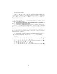
1) Sia dato il seguente modello di regressione lineare:
K variabili esplicative osservate. La variabile
se
y ≤ 0 ; y = 2 se
*
i
i
*
0 yi
< ≤ c ; y = 3 se
i
*
yi
*
i
y = x β + ε , i=1,…,N. Il vettore x i contiene
*
i i i
y non è osservabile. La variabile osservabile è y = 1
> c . 1.1) Di che tipo di modello si tratta 1.2) Scrivete
la funzione di verosimiglianza per il modello in questione. 1.3) Ipotizzate che il coefficiente β 2 sia
negativo. Quale sarà l’effetto di un aumento di x i2 su Prob(y i =1), Prob(y i =2) e Prob(y i =3)
2) Sia dato il seguente Linear Probability Model: yi = xiβ + εi
, i=1,…,N, dove il vettore x i contiene
K variabili esplicative osservate, mentre la variabile y
i
è una dummy binaria (0,1); i termini di
errore ε i sono distribuiti come una Normale con media nulla e varianza σ 2 . 2.1) Spiegate perché tale
modello non assicura che la probabilità stimata sia compresa tra 0 e 1. 2.2) Dimostrate che i termini
di errore ei sono eteroschedastici. 2.3) Ipotizzate che la variabile x i3 sia una dummy (0,1). Scrivete
l’espressione dell’effetto marginale relativo a tale variabile. 2.4) Ipotizzando N=100 e un numero di
osservazioni per cui y i =1 pari a 80, calcolate il valore della funzione di log verosimiglianza
massimizzata del modello ristretto yi
= β1
+ εi
.
3) Sia dato il seguente modello per dati panel:
K
it
= αi + ∑ β
r=
2 r rit
+
it
, i=1,…,N; t=1,…,T. 3.1)
y x u
Illustrate la procedura per ottenere le stime degli effetti individuali fissi α i . 3.2) Dimostrate come
ottenere stime degli effetti individuali casuali µ i . 3.3) Quali sono le analogie e le differenze tra lo
stimatore a effetti fissi e lo stimatore a effetti casuali
i
Gruppo 2 (40 punti)
Un ricercatore ha stimato un panel dinamico in cui il consumo industriale di carbone espresso in
logaritmi (lncoaltot) è funzione del logaritmo del valore aggiunto industriale espresso in termini
reali (lnrgdp95), di una serie di dummies temporali (y95-y02) e di una serie di dummies sulle zone
geografiche della Cina (z1-z6). I dati sono relativi a 27 province cinesi (i=1,…, N=27) aggregabili
in 6 zone e 6 anni (t=1,…, T=6).
I risultati della stima Arellano-Bond one-step sono riportati nella Tabella 1. Facendo riferimento a
tale tabella:
1

a) Interpretate il significato di: D.lncoaltot; lncoaltot LD; lngdp95 D1.
b) Per quale motivo la variabile z6 non compare tra i regressori
c) Spiegate qual è l’ipotesi nulla del test di Sargan riportato alla fine della Tabella 1. Perché la
distribuzione di tale test ha 20 gradi di libertà
d) Motivate la presenza dei due test di Arellano-Bond riportati in fondo alla Tabella 1.
e) Illustrate la differenza tra lo stimatore di Arellano-Bond one-step e lo stimatore di Arellano-Bond
two-step. Sotto quali circostanze usereste lo stimatore two-step
Tabella 1. Stima panel dinamico (Arellano-Bond one-step)
________________________________________________________________________________________________
Arellano-Bond dynamic panel-data estimation Number of obs = 162
Group variable (i): province Number of groups = 27
Wald chi2(12) = 49.54
Time variable (t): year Obs per group: min = 6
avg = 6
max = 6
One-step results
----------------------------------------------------------------------------------------------------------------------------
D.lncoaltot | Coef. Std. Err. z P>|z| [95% Conf. Interval]
--------------+-------------------------------------------------------------------------------------------------------------
lncoaltot |
LD | .3667676 .1480146 2.48 0.013 .0766642 .6568709
lngdp95 |
D1 | .0056595 .1174029 0.05 0.962 -.2244459 .2357648
y97 | -.0399372 .037185 -1.07 0.283 -.1128185 .032944
y98 | -.0265931 .0372111 -0.71 0.475 -.0995255 .0463394
y99 | -.0444324 .0377443 -1.18 0.239 -.1184099 .0295452
y00 | -.0272435 .0595839 -0.46 0.648 -.1440257 .0895388
y01 | .0194069 .0436269 0.44 0.656 -.0661003 .104914
z1 | .033142 .017536 1.89 0.059 -.001228 .0675119
z2 | .0001187 .0163511 0.01 0.994 -.0319288 .0321662
z3 | -.0051435 .016679 -0.31 0.758 -.0378337 .0275468
z4 | .0304122 .0154463 1.97 0.049 .000138 .0606863
z5 | .0093176 .0157389 0.59 0.554 -.02153 .0401653
_cons | -.0067297 .0273432 -0.25 0.806 -.0603215 .046862
------------------------------------------------------------------------------------------------------------------------------
Sargan test of over-identifying restrictions:
chi2(20) = 38.57 Prob > chi2 = 0.0075
Arellano-Bond test that average autocovariance in residuals of order 1 is 0:
H0: no autocorrelation z = -3.17 Pr > z = 0.0015
Arellano-Bond test that average autocovariance in residuals of order 2 is 0:
H0: no autocorrelation z = -0.24 Pr > z = 0.8130
________________________________________________________________________________________________
2