Appunti di Calcolo Numerico - Esercizi e Dispense - Università degli ...
Appunti di Calcolo Numerico - Esercizi e Dispense - Università degli ...
Appunti di Calcolo Numerico - Esercizi e Dispense - Università degli ...

You also want an ePaper? Increase the reach of your titles
YUMPU automatically turns print PDFs into web optimized ePapers that Google loves.
5. INTERPOLAZIONE<br />
Abbiamo quin<strong>di</strong> una formula per l’errore, detta anche formula del resto. Il resto normalmente è incognito<br />
ma se conosciamo la f e una maggiorazione della f (n+1) , allora possiamo maggiorare il resto.<br />
Allo stesso modo, possiamo limitare l’errore <strong>di</strong> interpolazione se troviamo un limite superiore per |F (x)|.<br />
Differenze<br />
<strong>di</strong>vise e<br />
formula <strong>di</strong><br />
Newton<br />
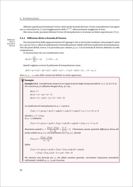
5.3.4 Differenze <strong>di</strong>vise e formula <strong>di</strong> Newton<br />
Uno dei punti forti della rappresentazione <strong>di</strong> Lagrange è che se alcuni dati cambiano (ad esempio il valore<br />
<strong>di</strong> y j per un certo j ) allora il cambiamento è imme<strong>di</strong>atamente visibile nell’intero polinomio <strong>di</strong> interpolazione.<br />
Uno dei punti deboli, invece, è la procedura per valutare p n (x). Con la formula <strong>di</strong> Newton abbiamo un utile<br />
compromesso.<br />
Le funzioni base che ora consideriamo sono<br />
j∏<br />
−1<br />
φ j (x) = (x − x i ) j = 0,1,...,n<br />
i=0<br />
Quin<strong>di</strong> vogliamo scrivere il polinomio <strong>di</strong> interpolazione come:<br />
p(x) = c 0 + c 1 (x − x 0 ) + c 2 (x − x 0 )(x − x 1 ) + ... + c n (x − x 0 )(x − x 1 ) · ...(x − x n−1 )<br />
dove c 0 , c 1 ...c n sono delle costanti da definire in modo opportuno.<br />
Esempio<br />
Esempio 5.3.4 Consideriamo sempre le tre coppie <strong>di</strong> punti <strong>degli</strong> esempi precedenti, (1,1), (2,3) e (4,3).<br />
Per costruire p 2 (x) abbiamo bisogno <strong>di</strong> φ 0 , φ 1 e φ 2 :<br />
φ 0 (x) = 1<br />
φ 1 (x) = (x − x 0 ) = (x − 1)<br />
φ 2 (x) = (x − x 0 )(x − x 1 ) = (x − 1)(x − 2)<br />
La con<strong>di</strong>zione <strong>di</strong> interpolazione in x 0 = 1 porta a:<br />
f (x 0 ) = 1 = p 2 (x 0 ) = p 2 (1) = c 0 φ 0 (1) + c 1 φ 1 (1) + c 2 φ 2 (1) = c 0 · 1 + c 1 · 0 + c 2 · 0<br />
Quin<strong>di</strong> c 1 = 1 = f (x 0 ).<br />
In x 1 = 2 abbiamo:<br />
f (x 1 ) = 3 = p 2 (x 1 ) = p 2 (3) = f (x 0 ) + c 1 φ 1 (2) + c 2 φ 2 (2) = f (x 0 ) + c 1 · 1 + c 2 · 0<br />
Ricaviamo quin<strong>di</strong> c 1 = f (x 1) − f (x 0 )<br />
= 3 − 1 = 2. Chiamiamo questa quantità <strong>di</strong>fferenza <strong>di</strong>visa del<br />
x 1 − x 0 2 − 1<br />
primo or<strong>di</strong>ne tra x 0 e x 1 e la in<strong>di</strong>chiamo con f [x 0 , x 1 ]. Quin<strong>di</strong><br />
Infine,<br />
f [x 0 , x 1 ] = f (x 1) − f (x 0 )<br />
x 1 − x 0<br />
f (x 2 ) = 3 = p 2 (x 2 ) = p 2 (4) = f (x 0 ) + f [x 0 , x 1 ]φ 1 (4) + c 2 φ 2 (4)<br />
= f (x 0 ) + f [x 0 , x 1 ](4 − 1) + c 2 (4 − 1)(4 − 2)<br />
Per ottenere una formula per c 2 che abbia carattere generale, riscriviamo l’equazione precedente<br />
utilizzando i simboli x 0 , x 1 , x 2 per le ascisse.<br />
68