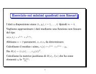
Appunti di Calcolo Numerico - Esercizi e Dispense - Università degli ...

10. INTEGRAZIONE NUMERICA
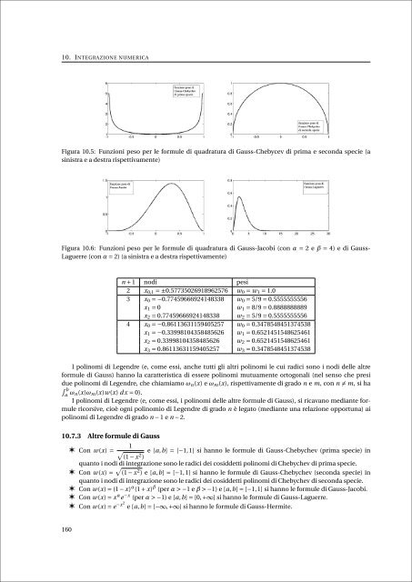
Figura 10.5: Funzioni peso per le formule di quadratura di Gauss-Chebycev di prima e seconda specie (a
sinistra e a destra rispettivamente)
Figura 10.6: Funzioni peso per le formule di quadratura di Gauss-Jacobi (con α = 2 e β = 4) e di Gauss-
Laguerre (con α = 2) (a sinistra e a destra rispettivamente)
n + 1 nodi pesi
2 x 0,1 = ±0.57735026918962576 w 0 = w 1 = 1.0
3 x 0 = −0.77459666924148338 w 0 = 5/9 = 0.5555555556
x 1 = 0 w 1 = 8/9 = 0.8888888889
x 2 = 0.77459666924148338 w 2 = 5/9 = 0.5555555556
4 x 0 = −0.86113631159405257 w 0 = 0.3478548451374538
x 1 = −0.33998104358485626 w 1 = 0.6521451548625461
x 2 = 0.33998104358485626 w 2 = 0.6521451548625461
x 3 = 0.86113631159405257 w 3 = 0.3478548451374538
I polinomi di Legendre (e, come essi, anche tutti gli altri polinomi le cui radici sono i nodi delle altre
formule di Gauss) hanno la caratteristica di essere polinomi mutuamente ortogonali (nel senso che presi
due polinomi di Legendre, che chiamiamo ω n (x) e ω m (x), rispettivamente di grado n e m, con n ≠ m, si ha
∫ b
a ω n(x)ω m (x)w(x) d x = 0).
I polinomi di Legendre (e, come essi, i polinomi delle altre formule di Gauss), si ricavano mediante formule
ricorsive, cioè ogni polinomio di Legendre di grado n è legato (mediante una relazione opportuna) ai
polinomi di Legendre di grado n − 1 e n − 2.
10.7.3 Altre formule di Gauss
1
G Con w(x) = √ e [a,b] = [−1,1] si hanno le formule di Gauss-Chebychev (prima specie) in
(1 − x 2 )
quanto i nodi di integrazione sono le radici dei cosiddetti polinomi di Chebychev di prima specie.
G Con w(x) = √ (1 − x 2 ) e [a,b] = [−1,1] si hanno le formule di Gauss-Chebychev (seconda specie) in
quanto i nodi di integrazione sono le radici dei cosiddetti polinomi di Chebychev di seconda specie.
G Con w(x) = (1 − x) α (1 + x) β (per α > −1 e β > −1) e [a,b] = [−1,1] si hanno le formule di Gauss-Jacobi.
G Con w(x) = x α e −x (per α > −1) e [a,b] = [0,+∞] si hanno le formule di Gauss-Laguerre.
G Con w(x) = e −x2 e [a,b] = [−∞,+∞] si hanno le formule di Gauss-Hermite.
160