Appunti di Calcolo Numerico - Esercizi e Dispense - Università degli ...
Appunti di Calcolo Numerico - Esercizi e Dispense - Università degli ...
Appunti di Calcolo Numerico - Esercizi e Dispense - Università degli ...

Create successful ePaper yourself
Turn your PDF publications into a flip-book with our unique Google optimized e-Paper software.
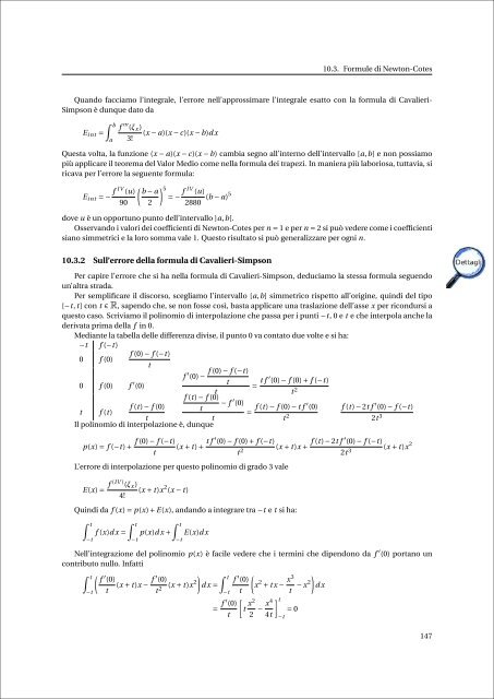
10.3. Formule <strong>di</strong> Newton-Cotes<br />
Quando facciamo l’integrale, l’errore nell’approssimare l’integrale esatto con la formula <strong>di</strong> Cavalieri-<br />
Simpson è dunque dato da<br />
∫ b<br />
E i nt =<br />
a<br />
f ′′′ (ξ x )<br />
(x − a)(x − c)(x − b)d x<br />
3!<br />
Questa volta, la funzione (x − a)(x − c)(x − b) cambia segno all’interno dell’intervallo [a,b] e non possiamo<br />
più applicare il teorema del Valor Me<strong>di</strong>o come nella formula dei trapezi. In maniera più laboriosa, tuttavia, si<br />
ricava per l’errore la seguente formula:<br />
E i nt = − f IV (u)<br />
90<br />
( ) b − a 5<br />
= − f IV (u)<br />
(b − a)5<br />
2 2880<br />
dove u è un opportuno punto dell’intervallo ]a,b[.<br />
Osservando i valori dei coefficienti <strong>di</strong> Newton-Cotes per n = 1 e per n = 2 si può vedere come i coefficienti<br />
siano simmetrici e la loro somma vale 1. Questo risultato si può generalizzare per ogni n.<br />
10.3.2 Sull’errore della formula <strong>di</strong> Cavalieri-Simpson<br />
Per capire l’errore che si ha nella formula <strong>di</strong> Cavalieri-Simpson, deduciamo la stessa formula seguendo<br />
un’altra strada.<br />
Per semplificare il <strong>di</strong>scorso, scegliamo l’intervallo [a,b] simmetrico rispetto all’origine, quin<strong>di</strong> del tipo<br />
[−t, t] con t ∈ R, sapendo che, se non fosse così, basta applicare una traslazione dell’asse x per ricondursi a<br />
questo caso. Scriviamo il polinomio <strong>di</strong> interpolazione che passa per i punti −t, 0 e t e che interpola anche la<br />
derivata prima della f in 0.<br />
Me<strong>di</strong>ante la tabella delle <strong>di</strong>fferenza <strong>di</strong>vise, il punto 0 va contato due volte e si ha:<br />
−t f (−t)<br />
f (0) − f (−t)<br />
0 f (0)<br />
t<br />
f ′ f (0) − f (−t)<br />
(0) −<br />
0 f (0) f ′ (0)<br />
t<br />
= t f ′ (0) − f (0) + f (−t)<br />
t<br />
t 2<br />
f (t) − f (0)<br />
− f<br />
f (t) − f (0)<br />
′ (0)<br />
t f (t)<br />
t<br />
= f (t) − f (0) − t f ′ (0) f (t) − 2t f ′ (0) − f (−t)<br />
t<br />
t<br />
t 2<br />
2t 3<br />
Il polinomio <strong>di</strong> interpolazione è, dunque<br />
f (0) − f (−t)<br />
p(x) = f (−t) + (x + t) + t f ′ (0) − f (0) + f (−t)<br />
t<br />
t 2 (x + t)x + f (t) − 2t f ′ (0) − f (−t)<br />
2t 3 (x + t)x 2<br />
L’errore <strong>di</strong> interpolazione per questo polinomio <strong>di</strong> grado 3 vale<br />
E(x) = f (IV ) (ξ x )<br />
(x + t)x 2 (x − t)<br />
4!<br />
Quin<strong>di</strong> da f (x) = p(x) + E(x), andando a integrare tra −t e t si ha:<br />
∫ t<br />
−t<br />
−t<br />
∫ t<br />
∫ t<br />
f (x)d x = p(x)d x + E(x)d x<br />
−t<br />
−t<br />
Nell’integrazione del polinomio p(x) è facile vedere che i termini che <strong>di</strong>pendono da f ′ (0) portano un<br />
contributo nullo. Infatti<br />
∫ t<br />
( f ′ (0)<br />
(x + t)x − f ′ ) ∫<br />
(0)<br />
t<br />
t<br />
t 2 (x + t)x 2 f ′ )<br />
(0)<br />
d x =<br />
(x 2 + t x − x3<br />
t<br />
t − x2 d x<br />
−t<br />
= f ′ (0)<br />
t<br />
[t x2<br />
2 − x4<br />
4t<br />
] t<br />
−t<br />
= 0<br />
147