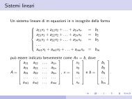
Approssimazione di funzioni e dati

Approssimazione di funzioni e dati
Dati
{x i , y i }, i = 1, . . .,N
x i ∈ [a, b], detti nodi o punti base, y i , valori ivi assunti da una f
non nota o ”difficile” da calcolare, si vuole trovare una F(x),
definita in [a, b] :
F(x i ) = y i .
La funzione F(x) potrà essere usata
• per interpolare i dati: stimare il valore assunto da f (x) in ogni
altro punto di [a, b]
• per estrapolare i dati: stimare il valore che f (x) assume in
punti esterni all’intervallo [a, b].
Il problema dell’estrapolazione è fortemente indeterminato, quello
dell’interpolazione è risolubile se si suppone f (x) sufficientemente
regolare nell’intervallo [a, b].

Dati, ad esempio,
x 0 1 2 3 4 5 6 7 8
f(x) 0.16 0.09 0.86 1.76 1.96 1.28 0.34 0.01 0.59
congiungendoli con una spezzata (spline lineare).
2
1.8
1.6
1.4
1.2
1
0.8
0.6
0.4
0.2
0
0 1 2 3 4 5 6 7 8
si ottiene una funzione interpolatrice continua ma non derivabile
nei nodi ⇒ molto sensibile agli errori nei dati.

In generale si sceglie come funzione interpolatrice
• una funzione ”semplice”, come un polinomio
• una funzione che coincida localmente con un polinomio (spline)
• In qualche caso è opportuno usare funzioni trigonometriche o
funzioni esponenziali.
• Se si suppone che f (x) sia una funzione di variabile aleatoria con
proprietà statistiche rilevabili dai dati osservati si puó ricorrere ai
metodi della Statistica.

Teorema di Lagrange
Data una funzione f (x) ∈ C n+1 ([a, b]), (continua con derivate
continue fino all’ordine n + 1 nell’intervallo [a, b] ed n + 1 coppie di
numeri reali
{x i , f (x i )}, i = 0, . . .,n con x i ∈ [a, b]
esiste uno ed un solo polinomio di grado n P L (x):
P L (x i ) = f (x i ).
P L (x) è detto polinomio interpolatore di Lagrange e soddisfa la
relazione
f (x) = P L (x) + R L (x)
R L (x) = f (n+1) (ξ x )
(n + 1)! (x − x 0)...(x − x n ), ξ ∈ [a, b].

Dimostrazione
La dimostrazione è costruttiva. Indichiamo con F(x) il polinomio
di grado n + 1 che si annulla in tutti i nodi
F(x) := ∏ n
i=0 (x − x i)
Per ogni k = 0, 1, 2, . . .,n, consideriamo
F k (x) =
F(x)
(x − x k )
F k (x k ) = ∏ n
i=0,i≠k (x k − x i ).
F k (x) é il polinomio di grado n che si annulla in tutti i nodi diversi
da x k ed F k (x k ) é il valore che esso assume per x = x k . Per ogni
k = 0, 1, . . .,n la funzione base relativa al nodo k-esimo è il
polinomio di grado n
L k (x) := F k(x)
F k (x k ) tale che L k(x i ) =
cioè vale uno nel nodo x k e zero negli altri.
{ 0 k ≠ i
1 k = i

Il polinomio
è di grado n e
P L (x) = L 0 (x)f (x 0 ) + L 1 (x)f (x 1 ) + . . . + L n (x)f (x n )
P L (x i ) = f (x i )
i = 0, 1, . . .,n.
Ogni altro polinomio di grado n che soddisfi queste relazioni ha
n + 1 radici in comune con P L (x) e quindi coincide con esso ⇒
P L (x) é il polinomio interpolatore di Lagrange.
Si dimostra che l’errore di interpolazione che si commette
prendendo P L (¯x) al posto di f (¯x) in un punto ¯x ∈ [a, b], diverso
dai nodi, é
R L (x) = f (n+1) (ξ¯x )
(n + 1)! (x − x 0)(x − x 1 )...(x − x n )
resto della formula di interpolazione di Lagrange.

R L (x) = f (n+1) (ξ¯x )
(n + 1)! (x − x 0)(x − x 1 )...(x − x n )
implica che l’ interpolazione di Lagrange è di ordine n, cioè esatta
per polinomi di grado n
Un polinomio di grado n ha la derivata n-esima sempre = 0.
Ha un valore soprattutto teorico, dato che non conosciamo ξ¯x .
Fornisce stime accettabili se f (n+1) è limitata in a, b.
N.B. Non si calcolano esplicitamente i coefficienti delle funzioni
base L k (x), ma, per ridurre l’influenza degli errori di
arrotondamento, si usano come prodotto di monomi.
Se si aggiungono punti ai dati {x i , y i := f (x i )}, i = 0, . . .n per
ottenere un polinomio interpolatore di grado più elevato, si devono
ricalcolare tutti i coefficienti.

Esempio
Le funzioni base relative ai nodi sono
x 0 1 2 4
y 0 6 8 48
(x − 1)(x − 2)(x − 4)
L 0 (x) = =
(−1)(−2)(−4)
(x − 0)(x − 2)(x − 4)
L 1 (x) =
(1 − 0)(1 − 2)(1 − 4)
x(x − 1)(x − 4)
L 2 (x) =
2(2 − 1)(2 − 4)
x(x − 1)(x − 2)
L 3 (x) =
4(4 − 2)(4 − 2)
(x − 1)(x − 2)(x − 4)
(−8)
=
x(x − 2)(x − 4)
3
=
x(x − 1)(x − 4)
(−4)
=
x(x − 1)(x − 2)
24
quindi il polinomio di Lagrange che interpola i dati osservati è
P(x) = L 0 (x) · 0 + L 1 (x) · 6 + L 2 (x) · 8 + L 3 (x) · 48
= 2x(x − 2)(x − 4) − 2x(x − 1)(x − 4) + 2x(x − 1)(x − 2).

0 0.5 1 1.5 2 2.5 3 3.5 4
50
45
40
35
30
25
20
15
10
5
0
Si ottiene, ad esempio f (1.75) ≃ P(1.75) = 7.21875.

Esercizio 2
Il polinomio di Lagrange di grado 8 che interpola i dati
x 0 1 2 3 4 5 6 7 8
f(x) 0.16 0.09 0.86 1.76 1.96 1.28 0.34 0.01 0.59
2
1.5
1
0.5
0
−0.5
0 1 2 3 4 5 6 7 8

50
45
40
35
30
25
20
15
10
5
0
0 0.5 1 1.5 2 2.5 3 3.5 4
Linea continua: polinomio interpolatore di Lagrange
Trattini: spezzata interpolatrice ( spline lineare )

2
1.8
1.6
1.4
1.2
1
0.8
0.6
0.4
0.2
0
0 1 2 3 4 5 6 7 8
Linea continua: polinomio interpolatore di Lagrange
Trattini: spezzata interpolatrice ( spline lineare )

Polinomio di Newton
Dati n + 1 valori {x i , y i } i=0,...,n , un metodo più efficiente per
determinare il polinomio interpolatore, cioé quel polinomio P(x) di
grado n che soddisfa tutte le relazioni P(x i ) = y i è il seguente.
p 0 (x) := y 0
soddisfa solo la prima relazione. Aggiungendo a p 0 un termine che
vale 0 in x 0 (in modo da salvare il risultato precedente) definiamo
p 1 (x) := p 0 (x) + t 1 (x − x 0 ), con t 1 := y 1 − y 0
x 1 − x 0
N.B. t 1 é tale che p 1 (x 1 ) = y 1 . Ora p 1 soddisfa le prime due
relazioni ma non le altre. Aggiungiamo un termine che valga 0 sia
in x 0 che in x 1
p 2 (x) = p 1 (x) + t 2 (x − x 0 )(x − x 1 ), t 2 :=
N.B. t 2 é tale che p 2 (x 2 ) = y 2 .
y 2 − p 1 (x 2 ))
8x 2 − x 1 )(x 2 − x 0 )

Al passo k
p k (x) = p k−1 (x) + t k (x k − x 0 )(x k − x 1 ) · · ·(x k − x k−1 )
t k :=
fino ad ottenere il
polinomio di Newton
y k − p k−1 (x k )
(x k − x 0 )(x k − x 1 ) · · ·(x k − x k−1 ) . . .
(∗) p N (x) = y 0 +t 1 (x −x 0 )+ . . . t n (x −x 0 )(x −x 1 ) · · ·(x −x n−1 ).
Dato che ha grado n e P N (x i ) = y i per i = 0, 1, . . .,n coincide
con il polinomio interpolatore di Lagrange.
Contrariamente a quanto succede per il polinomio di Lagrange,
l’introduzione di un nuovo punto comporta solo l’aggiunta di un
nuovo termine.

Differenze divise
I coefficienti del polinomio di Newton si possono calcolare anche
nel modo seguente.
def. Date n + 1 coppie di valori {(x i , f (x i ))} i=0,1,2,..n definiamo
• Differenze divise di ordine 1 f [x 0 , x 1 ] := f (x 1) − f (x 0 )
x 1 − x 0
,
• Diff. divise di ordine due f [x 0 , x 1 , x 2 ] := f [x 1, x 2 ] − f [x 0 , x 1 ]
x 2 − x 0
,
• Diff. divise di ordine n
f [x 0 , x 1 , . . .,x n ] := f [x 1, . . .,x n−1 ] − f [x 0 , . . .,x n−2 ]
x n−1 − x 0
.
Le differenze divise di ordine uno sono rapporti incrementali della
f (x), e quindi approssimazioni di f ′ (x), quelle di ordine due sono
rapporti incrementali del secondo ordine, etc. Si dimostra che
t i = f [x 0 , x 1 , . . .,x i ]
i = 0, 1, . . .,n.

Tabella delle differenze divise con n = 4
x 0 f (x 0 )
f [x 0 , x 1 ]
x 1 f (x 1 ) f [x 0 , x 1 , x 2 ]
f [x 1 , x 2 ] f [x 0 , x 1 , x 2 , x 3 ]
x 2 f (x 2 ) f [x 1 , x 2 , x 3 ] f [x 0 , x 1 , x 2 , x 3 , x 4 ]
f [x 2 , x 3 ] f [x 1 , x 2 , x 3 , x 4 ]
x 3 f (x 3 ) f [x 2 , x 3 , x 4 ]
f [x 3 , x 4 ]
x 4 f (x 4 )
Si ha
f [x i , x i+1 ] = f [x i+1 , x i ], i = 0, 1, . . .
e le differenze divise di ordine superiore non cambiano se gli
argomenti vengono permutati ⇒ si possono aggiungere nuovi punti
alla fine della tabella.

Il polinomio di Newton si può dunque scrivere anche nel modo
seguente.
p N (x) = f (x 0 ) + (x − x 0 )f [x 0 , x 1 ] + (x − x 0 )(x − x 1 )f [x 0 , x 1 , x 2 ]+
+... + (x − x 0 )...(x − x n−1 )f [x 0 , x 1 , x 2 , . . .,x n ]
Vale la relazione
f (x) = p N (x) + R N (x)
dove R N (x) é il resto della formula di Newton
e si ha
R N (x) := f [x 0 , x 1 , x 2 , ..,x n , x] ∏ n
i=0 (x − x i)
R N (x) = R L (x) = f (n+1) (ξ x ) ∏ n
(n + 1)!
(x − x i).
i=0

Esempio
x 0.9 1.1 1.3 1.5 1.7
f (x) 1.3784 1.4491 1.5166 1.5811 1.6432
I coefficienti del polinomio interpolatore di Newton sono gli elementi della
prima diagonale.
x f (x) f [x i ,x i+1 ] f [x i ,.,x i+2 ] f [x i ,.,x i+3 ] f [x i ,.,x i+4 ]
0.9 1.3784
0.3535
1.1 1.4491 −0.04
0.3375 4.167 · 10 − 3
1.3 1.5166 −0.0375 0.010417
0.3225 0.0125
1.5 1.5811 −0.03
0.3105
1.7 1.6432

Si ha
p 1 (x) = 1.3784 + 0.3535(x − 0.9)
p 2 (x) = p 1 (x) − 0.04(x − 0.9)(x − 1.1)
p 3 (x) = p 2 (x) + 4.167 · 10 −3 (x − 0.9)(x − 1.1)(x − 1.3)
p 4 (x) = p 3 (x) + 0.010417(x − 0.9)(x − 1.1)(x − 1.3)(x − 1.5)
p N (x) = 1.3784 + 0.3535(x − 0.9) − 0.04(x − 0.9)(x − 1.1)+
+4.167 · 10 −3 (x − 0.9)(x − 1.1)(x − 1.3)+
+0.010417(x − 0.9)(x − 1.1)(x − 1.3)(x − 1.5)
Ad es. per f (1) si ottengono le seguenti stime:
p 1 (1) = 1.41375 p 2 (1) = 1.41415
p 3 (1) = 1.4141625 p 4 (1) = 1.4141468745

In questo esempio accademico sappiamo che la funzione tabulata è
f (x) = √ 1 + x ed f (1) = √ 2 ≈ 1.41421356237309, quindi gli
errori si possono calcolare e valgono, rispettivamente
e 1 = 0.464 · 10 −3
e 2 = 0.64 · 10 −4
e 3 = 0.51 · 10 −4
e 4 = 0.67 · 10 −4
Si dimostra che l’interpolazione con polinomi di Lagrange su nodi
equidistanti è più accurata al centro dell’intervallo.

Accuratezza nell’interpolazione polinomiale
Volendo stimare il valore della funzione in un particolare punto,
anziché utilizzare un polinomio di grado elevato è meglio usarne
uno di grado piú basso, ma costruito su nodi che costituiscono un
intervallo simmetrico rispetto al punto da interpolare.
Viene spontaneo pensare che l’approssimazione sia tanto migliore
quanto più grande è il numero dei nodi e quindi quanto più è
elevato il grado del polinomio interpolatore. Ma non è così.
Il grafico dei polinomi interpolatori, al crescere del grado, presenta
oscillazioni di ampiezza crescente fra i valori nei nodi, con un
errore particolarmente alto in vicinanza degli estremi dell’intervallo.
Questo comportamento, dell’errore, detto fenomeno di Runge, è
tipico dell’interpolazione con polinomi di grado elevato quando i
nodi sono equidistanti e si può spiegare teoricamente.

Fenomeno di Runge
2
1.5
1
0.5
0
−0.5
−5 −4 −3 −2 −1 0 1 2 3 4 5
Un esempio classico é la funzione f (x) = 1
1 + x 2 nell’intervallo
[−5, 5]. Il grafico del polinomio P L (x) ottenuto interpolando i
valori di f nei nodi equidistanti {x i = −5 + i}, i = 0, . . .,10} .

Nodi di Chebyshev
Se i punti base per l’interpolazione in [−1 1] sono gli zeri del
polinomio di Chebyshev di grado n, detti nodi di Chebyshev
( 2k + 1
t k = − cos
n + 1 · π )
per k = 0, 1, . . .,n
2
l’ errore di interpolazione é uniforme su tutto l’intervallo.
Se x i ∈ [a, b], ed f (x) é nota analiticamente, il cambio di variabile
x =
(b − a) · t + (b + a)
2
fornisce i punti base per l’interpolazione,
per − 1 ≤ t ≤ 1
x k := b − a
2 t k + b + a
2
k = 1, ..n.

p C (x), il polinomio interpolatore di grado n basato sui nodi di
Chebychev, è, fra tutti i polinomi interpolatori di grado n, quello
per il quale è minimo il massimo errore di interpolazione. Inoltre
lim n→∞ p C (x) = f (x) uniformemente in a, b.
Nell’intervallo [−5, 5] i nodi di Chebishev sono
0.25
0.2
0.15
0.1
0.05
0
−0.05
−0.1
−0.15
−0.2
−0.25
−6 −4 −2 0 2 4 6
I nodi di Chebyshev sono più fitti in prossimità degli estremi
dell’intervallo.

Il grafico del polinomio che interpola i valori di f (x) = 1
1+x 2
nell’intervallo [−5, 5] sui nodi di Chebyshev
1.2
1
0.8
0.6
0.4
0.2
0
−0.2
−5 −4 −3 −2 −1 0 1 2 3 4 5

Commenti
• Per poter utilizzare l’interpolazione di Chebyshev bisogna
conoscere analiticamente la funzione da interpolare.
• Se si hanno molti nodi equidistanti è preferibile usare più
polinomi interpolatori di grado non troppo elevato, basati su nodi
che costituiscono intervalli il più possibile simmetrici rispetto ai
punti da interpolare oppure funzioni interpolatrici ”polinomiali
tratti” (splines).

Derivazione numerica
Se f è una funzione definita tramite una tabella a punti
equidistanti e si vuole stimare f ′ in pochi punti. Sia f ∈ C 3 ([a, b]).
Dallo sviluppo in serie di Taylor
f (x + h) = f (x) + hf ′ (x) + h2
2 f ′′ (x) + h3
3! f (3) (x) + . . .
si ottiene
f ′ f (x + h) − f (x)
(x) = − h h 2 f ′′ (ξ).
Introducendo ∆, l’operatore delle differenze in avanti
(∆f )(x) := f (x + h) − f (x),
si può ricavare una stima di f ′ (x) tramite un rapporto incrementale
basato sulle differenze in avanti
f ′ (∆f )(x)
(x) ≈
h
che fornisce un’approssimazione di ordine uno, dato che l’errore è
nullo per polinomi di grado uno.

Dallo sviluppo in serie di Taylor
f (x − h) = f (x) − hf ′ (x) + h2
2 f ′′ (x) − h3
3! f (3) (x) + . . .
si ottiene
f ′ f (x) − f (x − h)
(x) = + h h 2 f ′′ (ξ).
Introducendo ∇, l’operatore delle differenze all’indietro,
(∇f )(x) := f (x) − f (x − h),
si ottiene la seguente stima, anch’essa di ordine uno.
f ′ (x) ≈
(∇f )(x)
.
h

Sottraendo membro a membro i due sviluppi in serie di Taylor si
ottiene
e quindi
f (x + h) − f (x − h) = 2hf ′ (x) + h3
3 · f (3) (ξ)
f ′ (x) =
f (x + h) − f (x − h)
2h
− h2
6 f (3) (ξ).
Introducendo δ, l’operatore delle differenze centrali,
(δf )(x) := f (x + h) − f (x − h),
si può ricavare una stima di f ′ con un’accuratezza di ordine due
f ′ (x) ≈
(δf )(x)
2h

Esercizio
Stimare f ′ (4.5) dove f è la funzione definita dalla seguente tabella.
x 4 4.25 4.5 4.75 5
y 0.027 0.166375 0.512 1.157625 2.197
I dati della tabella ci consentono di stimare f ′ (4.5) tramite ∆, ∇ e
δ, con h = 0.25 ottenendo :
f (4.75) − f (4.5)
F ∆ (h) = = 2.5825
0.25
f (4.5) − f (4.25)
F ∇ (h) = = 1.3825
0.25
f (4.75) − f (4.25)
F δ (h) = = 1.9825
0.5
Sapendo che la funzione tabulata è f (x) = (x − 3.7) 3 , si ha
f ′ (4.5) = 1.92, quindi l’errore sulle varie stime è il seguente.
e ∆ = −0.6625, e ∇ = 0.5375 e e δ = −0.0625.

Estrapolazione di Richardson
Supponiamo che F(h) indichi il valore di una certa quantità
ottenuta con passo h, ad esempio la stima della derivata in un
punto con ∆, e che si conosca l’andamento dell’errore al variare di
h, potendo scrivere
a 0 = F(h) + a 1 h p + O(h r ), (h → 0, r > p)
dove a 0 è la quantità che cerchiamo di calcolare.
Applicando la formula con un passo q · h, si ottiene
a 0 = F(qh) + a 1 (qh) p + O(h r ).
Sottraendo membro a membro si ha
0 ≈ F(h) + a 1 h p − F(qh) − a 1 q p h p .
Si ricava la seguente stima per il primo termine di errore
a 1 h p F(h) − F(qh)
≈
q p − 1
e quindi una nuova stima, più accurata, è

Nel caso della stima di f ′ (x) tramite le differenze centrali si ottiene
f ′ (x) = F 1 (h) = F δ (h) + a 1 h 2 + a 2 h 4 + . . .
f ′ (x) = F 1 (2h) = F δ (2h) + a 1 · 4h 2 + a 2 · 16h 4 + . . ..
Di conseguenza
a 1 h 2 ≈ F 1(h) − F 1 (2h)
3
F 2 (h) := F 1 (h) + F 1(h) − F 1 (2h)
3
Continuando il procedimento da
f ′ (x) = F 2 (h) + a 2 h 4 + . . .
f ′ (x) = F 2 (2h) + a 2 · 16h 4 + . . .

si ottiene
a 2 h 4 ≈ F 2(h) − F 2 (2h)
15
F 3 (h) := F 2 (h) + F 2(h) − F 2 (2h)
.
15
Le stime fornite dai vari F i (h) sono via via più accurate, dato che
f ′ (x) = F 1 (h) + O(h 2 )
= F 2 (h) + O(h 4 )
= F 3 (h) + O(h 6 )....

Esempio
Riprendendo l’esempio precedente, da
F 1 (h) =
f (4.75) − f (4.25)
0.5
= 1.9825
F 1 (2h) =
si ottiene la stima dell’errore
f (5) − f (4)
1
a 1 h 2 ≈ F 1(h) − F 1 (2h)
3
ed una stima più accurata per la derivata
= 2.17
= −0.0625
f ′ (4.5) ≈ F 2 (h) = F 1 (h)+ F 1(h) − F 1 (2h)
3
= 1.9825−0.0625 = 1.92
con un errore dell’ordine di h 4 ≈ 0.25 4 = 0.39 · 10 −2 .