Lo Standard JPEG per la Compressione di Immagini Fisse - InfoCom

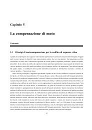
Capitolo 3
Lo Standard JPEG per la Compressione di
Immagini Fisse
Contenuto
3.1 Introduzione . . . . . . . . . . . . . . . . . . . . . . . . . . . . . . . . . . . . . . . . . . . . . . 48
3.2 Modalità Sequenziale . . . . . . . . . . . . . . . . . . . . . . . . . . . . . . . . . . . . . . . . . 50
3.2.1 Trasformata Dicreta del Coseno (DCT) . . . . . . . . . . . . . . . . . . . . . . . . . . . . 50
3.2.2 Quantizzatore . . . . . . . . . . . . . . . . . . . . . . . . . . . . . . . . . . . . . . . . . . 52
3.2.3 Codificatore Entropico . . . . . . . . . . . . . . . . . . . . . . . . . . . . . . . . . . . . . 53
3.2.4 Decodificatore . . . . . . . . . . . . . . . . . . . . . . . . . . . . . . . . . . . . . . . . . . 55
3.3 Modalità Progressiva . . . . . . . . . . . . . . . . . . . . . . . . . . . . . . . . . . . . . . . . . . 56
3.4 Modalità Gerarchica . . . . . . . . . . . . . . . . . . . . . . . . . . . . . . . . . . . . . . . . . . 58
3.1 Introduzione
Lo standard JPEG3.1 è forse il più diffuso standard di compressione per immagini fisse. Tale diffusione è dovuta
principalmente al fatto che tale standard permette di ottenere alti rapporti di compressione su immagini naturali a
frote di una perdita di qualità generalmente contenuta entro limiti accettabili.
Occorre, inoltre, tenere in considerazione il fatto che lo standard è “aperto”, nel senso che chiunque può
liberamente implementare il proprio codificatore/decodificatore JPEG.
Il numero massimo di componenti, o canali, costituenti l’immagine è fissato in 255.
3.1Joint Photographic Experts Group, ufficialmente ISO/JTC1/SC2/WG10, operante in stretta, informale, collaborazione con il gruppo
CCITT/SGVIII. L’attributo joint si riferisce proprio a questa collaborazione tra ISO (International Standard Organization) e CCITT (Commitee
Consultatif Internationale des Telephones et Telegraphs). Dal 1992, l’organismo ITU (International Telecommunication Union) raccoglie le
attività del CCCIT, del CCIR (Commitee Consultatif Internationale des Radio), del IFRB (International Frequency Registration Board), e del BDM
(Bureau des Developpement des Telecommunications).
48

3.1. INTRODUZIONE 49
Un’immagine a colori è rappresentata mediante tre canali, tipicamente uno di luminanza (Y ), e due di crominanza
(CR,CB). 3.2
Figura 3.1: Sottocampionamento della crominanza. Il simbolo X rappresenta un generico campione di luminanza, i due semiquadrati
rappresentano una coppia di campioni CRCB condivisa da quattro campioni di luminanza.
La crominanza è sottocampionanta di un fattore 2 in entrambe le direzioni, e quindi quattro pixel di luminanza
condividono la stessa crominanza, vedi Fig.3.1.
Modalità di funzionamento
Lo standard JPEG prevede quattro distinte modalità di funzionamento:
• Sequenziale (con DCT, con perdita);
• Progressiva (con DCT, con perdita);
• Senza Perdita;
• Gerarchica (con o senza DCT, con o senza perdita).
3.2 Dai coefficienti tricromatici del sistema di riferimento colorimetrico NTSC, i.e. RN ,GN ,BN , la trasformazione in luminanza/crominanza
si ottiene nel modo seguente:
Y =0.299 · RN +0.587 · GN +0.114 · BN
CR = RN − Y
CB = BN − Y
;
RN = CR + Y
BN = CB + Y
GN = Y − 0.299 · RN − 0.114 · BN
0.587
(3.1.1)

50 CAPITOLO 3. LO STANDARD JPEG PER LA COMPRESSIONE DI IMMAGINI FISSE
3.2 Modalità Sequenziale
blocco 8x8
Immagine
Originale
xn [ , n ]
DCT
1 2 X k1 k2
DCT
( ) [ , ]
Quantizzatore
( DCT)
X [ k , k ]
1 2
Codificatore
Entropico
Tavole Tavole
Figura 3.2: Schema del Codificatore JPEG
Dati Immagine
Compressa
La struttura essenziale di un codificatore JPEG è mostrata nella Fig.3.2. Ogni componente dell’immagine da codificare
è suddivisa in blocchetti da 8x8 pixel. Secondo una scansione lessicografica, ciascuno di questi blocchetti è elaborato
dalla trasformazioni indicate come DCT, Quantizzatore, Codificatore Entropico.
3.2.1 Trasformata Dicreta del Coseno (DCT)
Questa trasformazione opera il calcolo della DCT. Lo standard non specifica un particolare algoritmo di calcolo,
lasciando così a chi sviluppa il codificatore la libertà di implementare un particolare procedimento. Ciò dipende dal
fatto che diverse applicazioni possono richiedere differenti realizzazioni del calcolatore di DCT, e.g. realizzazioni
hardware VLSI rispetto a realizzazioni software o ibride come un DSP dedicato, implementazioni in artimetica a
virgola fissa o mobile, etc., ciascuna con differenti compromessi fra velocità e precisione.
Tale flessibilità può però presentare qualche svantaggio. In effetti, idealmente, la cascata di una trasformazione
DCT e di una trasformazione DCT inversa (IDCT) non comporta alcuna perdita di informazione. In realtà, la
presenza di funzioni sinusoidali nell’espressione della trasformata, rende impossibile di fatto realizzare i calcoli con
accuratezza perfetta. Dunque potremmo trovarci di fronte al problema che codificatori e decodificatori diversi, in
linea di principio, potrebbero produrre risultati anche abbastanza diversi fra loro. Per evitare tale problema, nello
standard JPEG sono specificati dei test di conformità rispetto all’accuratezza cui si devono adeguare il codificatore
e il decodificatore.
In ogni caso, ricordiamo le definizioni della DCT di un’immagine x[n1,n2] di dimensioni N ×N.
• Trasformata DCT (analisi):
X DCT N−1 X
[k1,k2] =α(k1)α(k2)
con α(0) def
q
1 = N e α(k) =
• Trasformata IDCT (sintesi):
x[n1,n2] =
N−1 X
N−1 X
k1=0 k2=0
N−1 X
n1=0 n2=0
q
2
N
µ µ
π(2n1 +1)k1 π(2n2 +1)k2
x[n1,n2]cos
cos
2N
2N
per 1 ≤ k ≥ N − 1;
α(k1)α(k2)X (DCT) µ µ
π(2n1 +1)k1 π(2n2 +1)k2
[k1,k2]cos
cos
2N
2N
0 ≤ k1,k2 ≤ N − 1
0 ≤ n1,n2 ≤ N − 1
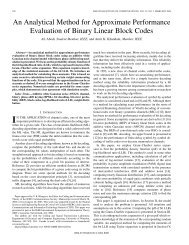
Dalle Figg. 3.3, 3.4, e 3.5 è possibile apprezzare come la DCT compatti l’energia media nelle componenti a bassa
frequenza. In tali figure, l’ampiezza dei coefficienti DCT é rappresentato come livelli di grigio, dal nero verso il
bianco.
Tale compattazione è ancora più evidente per blocchetti di dimensione contenuta (vedi Figg. 3.4 e 3.5), dove
la correlazione tra i pixel cresce, e l’approssimazione DCT → KLT è sufficientemente accurata. Si osservi come,
bastano pochissimi coefficienti DCT per “spiegare” blocchetti con scarse variazioni del livello di grigio.

3.2. MODALITÀ SEQUENZIALE 51
Figura 3.3: Immagine e relativa DCT
Figura 3.4: Immagine blocchettizzata (32x32) e relativa DCT
Figura 3.5: Immagine blocchettizzata (8x8) e relativa DCT

52 CAPITOLO 3. LO STANDARD JPEG PER LA COMPRESSIONE DI IMMAGINI FISSE
3.2.2 Quantizzatore
All’ingresso del quantizzatore si presentano dunque i 64 coefficienti estratti mediante DCT. Occorre ricordare che
fino all’ingresso del quantizzatore non vi è stata ancora alcuna perdita di informazione.
L’operazione di quantizzazione è definita nel modo seguente, per k1,k2 =0, ··· , 7:
˙X (DCT) µ
(DCT) X [k1,k2]
[k1,k2] =round
(3.2.1)
Q[k1,k2]
dove Q[k1,k2] sono i valori dei passi di quantizzazione associati a ciascun coefficiente DCT. La strategia adottata è
infatti quella di quantizzare ciascun coefficiente con uno specifico passo di quantizzazione, dipendente dall’importanza
psicovisiva che tale coefficiente possiede.
Le immagini naturali hanno un contenuto frequenziale rilevante che si situa nella massima parte alle basse
frequenze; conseguentemente, tra i 64 coefficienti DCT assumono valore significativamente diverso da zero solo
quelli concentrati intorno alle basse frequenze spaziali.
Poichè il sistema visivo umano è molto meno sensibile alle alte frequenze (che contengono l’informazione relativa
ai dettagli fini, alla tessitura, etc.) che alle basse; fra queste ultime, il coefficiente della componente continua (DC)
X (DCT) [0, 0], che rappresenta in sostanza il livello medio di grigio presente nel blocchetto 8x8, è quello che riveste
la maggiore importanza visuale. Per tali motivi, la quantizzazione è studiata per cercare di preservare (quantizzando
meno) il coefficiente DC, e in generale tutti quelli pertinenti alle basse frequenze, e invece quantizzare più duramente i
coefficienti corrispondenti alle alte frequenze. In pratica, i coefficienti corrispondenti alle alte frequenze spaziali, che
assumono valori relativamente piccoli, sono divisi per un valore di quantizzazione relativamente grande, tipicamente
compreso fra 80 e 100, e poi arrotondati all’intero più vicino, risultando così in un valore nullo. L’operazione di
quantizzazione, operazione irreversibile, provoca la perdita di informazione.
Le tabelle che contengono gli 8x8 valori dei passi di quantizzazione sono specificate dallo standard e sono state
ottenute in base ai risultati di numerosissime prove soggettive effettuate negli anni, ma viene in ogni caso lasciata la
possibilità al progettista del codificatore di specificarne di proprie, in quanto lo standard stesso prevede che le tabelle
debbano in ogni caso essere inserite nei dati codificati per essere comunicate al decodificatore.
Luminanza (Y )
16 11 10 16 24 40 51 61
12 12 14 19 26 58 60 55
14 13 16 24 40 57 69 56
14 17 22 29 51 87 80 62
18 22 37 56 68 109 103 77
24 35 55 64 81 104 113 92
49 64 78 87 103 121 120 101
72 92 95 98 112 100 103 99
Crominanza (CRCB)
17 18 24 47 66 99 99 99
18 21 26 66 99 99 99 99
24 26 56 99 99 99 99 99
47 66 99 99 99 99 99 99
66 99 99 99 99 99 99 99
99 99 99 99 99 99 99 99
99 99 99 99 99 99 99 99
99 99 99 99 99 99 99 99
Tabella 3.1: Tabelle dei passi di quantizzazione Q[k1,k2] suggerite nello standard JPEG.
Una ultima considerazione riguarda i parametri resi disponibili all’utente per adattare il livello di compressione, e
quindi di qualità, alla particolare applicazione. In sostanza tale adattamento viene effettuato mediante la scalatura
tramite un coefficiente moltiplicativo dell’intera tabella di quantizzazione.
Prima di pervenire al codificatore entropico, i dati vengono riordinati nel seguente modo: i coefficienti DC di
ciascun blocchetto, essendo i livelli medi di grigio di ciascun blocchetto abbastanza correlati fra loro per immagini
naturali, saranno codificati come differenza fra il coefficiente DC del blocchetto corrente e quello del blocchetto
def
precedente, i.e. sarà codificata la differenza ∆DCi = DCi − DCi−1, inizializzata con DC0 =0.

3.2. MODALITÀ SEQUENZIALE 53
I restanti coefficienti, detti coefficienti AC per contrasto al coefficiente DC, sono poi scanditi a “zig-zag”, come
mostrato in Fig.3.6.
Figura 3.6: Coefficienti DC ed AC, preparazione alla codifica
Questa scansione trasforma i dati da matrici 8x8 in stringhe caratterizzate dall’avere i valori più significativi nelle
prime posizioni, per poi proseguire con lunghe corse di zeri.
3.2.3 Codificatore Entropico
Le stringhe di dati provenienti dal quantizzatore sono sottoposte ad un processo di codifica entropica, senza perdite.
Il processo di codifica è strutturato in 2 passi. Nel primo passo si converte la sequenza di coefficienti quantizzati
in una sequenza intermedia di simboli. Nel secondo passo si codificano i simboli intermedi in stringhe di cifre binarie
che costituiscono il vero e proprio “data stream”.
Primo passo: rappresentazione intermedia dei simboli
La sequenza di simboli intermedi è costruita nel seguente modo: ogni coefficiente AC non nullo è codificato
congiuntamente con la lunghezza della corsa di coefficienti nulli che lo precedono nella sequenza.
Ogni combinazione corsa/coefficiente non nullo è rappresentata mediante una coppia di simboli secondo lo schema
di Fig.3.7.
Simbolo-1 (8 cifre binarie) Simbolo-2 (SIZE cifre binarie)
RUNLEGTH SIZE
AMPLITUDE
4
4
Figura 3.7: Struttura della codifica entropica delle corse dei coefficienti AC: Simbolo-1 e Simbolo-2.
Il primo simbolo codifica due distinte informazioni, RUNLENGTH e SIZE; il secondo ne codifica una sola, AM-
PLITUDE, che rappresenta proprio il valore del coefficiente AC, non nullo, che termina la corsa. Poichè i valori dei
pixel dell’immagine x[n1,n2] sono rappresentati in virgola fissa con 8 cifre binarie, dalla relazione di trasformata
SIZE

54 CAPITOLO 3. LO STANDARD JPEG PER LA COMPRESSIONE DI IMMAGINI FISSE
DCT si vede che sono necessari 11 cifre binarie per rappresentare il valore del generico coefficente AC, sia prima
che dopo la quantizzazione.
Il campo SIZE rappresenta il numero di cifre binarie utilizzato per codificare il campo AMPLITUDE, cioè per
codificare il Simbolo-2, secondo lo schema di Tab.3.2.
SIZE AMPLITUDE
1 1, -1
2 -3, -2, 2, 3
3 -7, -6, -5, -4, 4, 5, 6, 7
4 -15, ···, -8, 8, ···,15
5 -31, ···, -16, 16, ···,31
6 -63, ···, -32, 32, ···,63
7 -127, ···, -64, 64, ···, 127
8 -255, ···, -128, 128, ···,255
9 -511, ···, -256, 256, ···,511
10 -1023, ···, -512, 512, ···,1023
11 -2047, ···, -1024, 1024, ···, 2047
Tabella 3.2: Codifica del Simbolo-2
Lo schema comprende anche il valore SIZE=11, necessario per rappresentare la differenza ∆DCi = DCi − DCi−1.
Il campo RUNLENGTH rappresenta corse di zeri di lunghezze comprese fra 0 e 15, per cui occorrono 4 cifre
binarie per la sua translitterazione. Poichè la lunghezza delle corse può, e sperabilmente deve, superare il valore 15,
il valore speciale (15, 0) di Simbolo-1 è utilizzato come simbolo estensione della lunghezza di corsa (corsa lunga
almeno 16). Poiché abbiamo 63 coefficienti AC, si possono incontrare fno ad un massimo di tre simboli estensione,
oltre ad un Simbolo-1 detto terminatore, il cui campo RUNLENGTH completa la lunghezza totale della corsa. Per
esempio, i tre Simboli-1 consecutivi, con relativo Simbolo-2, (15, 0)(15, 0)(3, 4)(11) rappresentano una corsa lunga
16+16+3=35 coefficienti AC nulli, terminata da un Simbolo2 di SIZE=4 cifre binarie, con AMPLITUDE=6.
Il Simbolo-1 terminatore è sempre seguito da un singolo Simbolo-2, eccetto il caso nel quale oltre un certo
coefficiente vi siano solo zeri: in tale caso, il valore speciale (0, 0) di Simbolo-1 viene specificato per rappresentare
la fine dei dati pertinenti al blocchetto considerato.
Per quanto riguarda il valore differenziale del coefficiente DC, la rappresentazione intermedia è simile al caso
AC, con la differenza che Simbolo-1 comprende solo il campo SIZE con valori fra 1 e 11, come mostrato in Fig.3.8.
Simbolo-1 (4 cifre binarie) Simbolo-2 (SIZE cifre binarie)
SIZE
4
AMPLITUDE
Figura 3.8: Struttura della codifica entropica dei coefficienti ∆DCi: Simbolo-1 e Simbolo-2.
Un possibile esempio di stringa codificata intermedia è dunque il seguente:
SIZE
(2)(3),(0, 8)(116),(0, 6)(37),···,(12, 4)(12),(15, 0)(15, 0)(2, 2)(3),(0, 0)
La struttura di Simbolo-1 è riassunta nella Tab.3.3

3.2. MODALITÀ SEQUENZIALE 55
RUNLENGTH/SIZE 0 1 2 ... 10 11
0 EOB ...
1 X ...
. X valori legali di SIZE
. X ...
15 ZRL ...
Tabella 3.3: Struttura del Simbolo-1 con i simboli speciali di fine blocchetto (EOB) ed estensione di corsa (ZRL).
Secondo passo: codifica a lunghezza di parola variabile
Una volta creata la sequenza intermedia, a essa vengono associate le effettive parole di codice.
Ogni Simbolo-1 è codificato mediante una parola di codice a lunghezza variabile (Variable Length Code, VLC)
ottenuta mediante codifica di Huffman. Il relativo Simbolo-2 è codificato mediante un cosiddetto intero di lunghezza
variabile (Variable Length Integer, VLI) la cui lunghezza è specificata dal campo SIZE del Simbolo-1. La parola VLI
si ottiene come segue: per ogni “piano” individuato dal valore di SIZE, si effettua una translitterazione con parole di
codice di lughezza pari proprio a SIZE. Un esempio relativo a SIZE=3 é riportato in Tab.3.4.
AMPLITUDE -7 -6 -5 -4 4 5 6 7
Parola di Codice 000 001 010 011 100 101 110 111
Tabella 3.4: Translitterazione del campo AMPLITUDE (SIZE=3).
Sia i VLC che i VLI sono codici a lunghezza di parola variabile, ma solo i VLC sono codici di Huffman. Un fatto
notevole è che la lunghezza di un VLC non è nota finchè la parola non è stata decodificata, mentre la lunghezza di
un VLI è contenuta nel VLC precedente: la coppia VLC e VLI costituisce una parola di un codice concatenato.
3.2.4 Decodificatore
Il decodificatore, come mostrato nello schema qui di seguito riportato, è cosituito da blocchi analoghi a quelli del
codificatore.
Dati Immagine
Compressa
Decodificatore
Entropico
Tavole
( DCT)
X [ k , k ]
1 2
De-Quantizzatore
Tavole
( DCT)
X [ k , k ]
1 2
IDCT
Figura 3.9: Schema del Decodificatore JPEG
xn [ 1, n2]
Immagine
Ricostruita
Il decodificatore entropico rimappa, mediante le tavole comunicate con i dati, lo stream di cifre binarie in simboli
intermedi e da questi in valori quantizzati.
Dopo aver calcolato i coefficienti DC, i.e.
DCi = DCi−1 + ∆DCi

56 CAPITOLO 3. LO STANDARD JPEG PER LA COMPRESSIONE DI IMMAGINI FISSE
il de-quantizzatore ripristina la dinamica moltiplicando ciascun coefficiente DCT per il relativo coefficiente di
quantizzazione, comunicato con i dati, i.e.
ˆX (DCT) [k1,k2] = ˙X (DCT) [k1,k2] · Q[k1,k2]
La trasformazione IDCT opera il calcolo della Trasformata Coseno Discreta Inversa, ottenendo i campioni del
blocchetto ˆx[n1,n2], affetti dalla distorsione introdotta nella codifica.
Infine, l’immagine completa si ottiene posizionando correttamente, secondo un ordine lessicografico, tutti i
blocchetti 8x8.
3.3 Modalità Progressiva
Tale modalità è impiegata quando si voglia trasferire una immagine codificata su un canale a basso bit-rate, in
quanto consente di trasferire rapidamente una versione a bassa qualità dell’immagine, e.g. per renderla subito visibile
all’utente, e di raffinarla per passi successivi.
Sostanzialmente, in fase di codifica, i coefficienti DCT vengono codificati in gruppi successivi, e tali gruppi
sono poi inviati in successione attraverso il canale; tipicamente i gruppi di coefficienti sono selezionati in base alla
loro importanza psicovisiva, e dunque il primo gruppo comprende il coefficiente DC (livello medio di grigio del
blocchetto) e alcuni coefficienti AC.
L’immagine decodificata dalla ricezione di (solo) tale gruppo si presenterà come un insieme di blocchi uniformi;
aggiungendo un secondo gruppo di coefficienti AC, il dettaglio dell’immagine aumenterà, e così via fino a raggiungere
il livello corrispondente a quello ottenibile mediante la modalità sequenziale.
La modalità progressiva si articola in due metodi complementari:
• selezione spettrale;
• approssimazioni successive.
DCT
0
1
2
62
63
MSB
BLOCCHI
LSB
Figura 3.10: Rappresentazione numerica dei coefficienti DCT per i vari blocchetti di un’immagine.
Con riferimento alla Fig.3.10, dove la rappresentazione numerica dei coefficienti DCT dei vari blocchetti è illustrata
in modo tridimensionale, i metodi di selezione spettrale e approssimazioni successive sono illustrati in Fig.3.11.

3.3. MODALITÀ PROGRESSIVA 57
0
1
2
3
4
5
61
62
63
BLOCCHI
prima scansione
seconda scansione
ultima scansione
SELEZIONE SPETTRALE
11 10
BLOCCHI
prima scansione
9 8
seconda scansione
1
ultima scansione
APPROSSIMAZIONI SUCCESSIVE
Figura 3.11: Rappresentazione numerica dei coefficienti DCT per i vari blocchetti di un’immagine nelle modalità progressive
selezione spettrale e approssimazioni successive.

58 CAPITOLO 3. LO STANDARD JPEG PER LA COMPRESSIONE DI IMMAGINI FISSE
3.4 Modalità Gerarchica
Tale modalità rappresenta una alternativa alla realizzazione della modalità progressiva, e si basa sulla codifica di una
immagine come successione di immagini a risoluzione via via crescente.
M:1 =
2 / M
2
2 / M
b g F H G I K J F H G I K J
j j
1 2 1mod 2
2mod
2
He , e rect
rect
2M
2M
Figura 3.12: Sottocampionamento bidimensionale.
Il termine risoluzione si riferisce al contenuto di frequenze spaziali dell’immagine. L’operazione di sottocampionamento,
ottenuta per filtraggio e decimazione3.3 come illustrato in Fig.3.12 definisce il contenuto di frequenze spaziali
dell’immagine da codificare. Il filtraggio è necessario per evitare l’introduzione di distorsione da aliasing nella
successiva operazione di decimazione.
1:P =
PB
1
2 / P
MB
b g F H G I K J F H G I K J
j j
1 2 2 1mod 2
2mod
2
He , e P rect
rect
2P
2P
Figura 3.13: Interpolazione bidimensionale.
L’operazione di interpolazione, ottenuta per espansione3.4 e filtraggio come illustrato in Fig.3.13, ripristina soltanto
le corrette dimensioni dell’immagine, che risulta comunque a banda limitata (non pienamente risoluta). Il guadagno
del filtro recupera lo scalamento introdotto da precedenti operazioni di sottocampionamento.
3.3 L’operazione di decimazione di un fattore M in entrambe le dimensioni è definita come segue:
xd[n1,n2] def
= x[n1 · M, n2 · M]
3.4L’operazione di espansione di un fattore P in entrambe le dimensioni è definita come segue:
xe[n1,n2] def
⎧
⎨x[n1/P,
n2/P ] per n1,n2 =0 modP (n1 e n2 multipli di P )
=
⎩0
per n1,n2 = 0 modP (n1 e n2 non multipli di P )
2
2 / P
1

3.4. MODALITÀ GERARCHICA 59
La Fig.3.14 mostra un esempio di funzionamento dove codificatori con diverso bit-rate (qualità) sono impiegati
per le diverse “trasmissioni”.
xn [ , n ] 1.2 bit/pixel
prima trasmissione
1 2
1.2/16 = 0.075 bit/pixel
4:1 Cod-1
Decod-1
1:4
2:1
Decod-1
_
1:2
+
r42 , n1n2 [ , ]
[ n1, n2]
_
+
r , n n [ , ]
21 1 2
[ n1, n2]
_
+
Cod-1
Cod-2
seconda trasmissione
1.2/4 = 0.3 bit/pixel
Decod-1
+
+
1:2
Decod-2
+
+
Decod-1
terza trasmissione
0.5 bit/pixel
Decod-2
1:2
[ n1, n2]
rn [ , n ] xn [ , n ] xn
[ , n ]
1 2 1 2 1 2
+
+
+
+
[ n1, n2]
Figura 3.14: Funzionamento della modalità gerarchica.
1:2
0.075 bit/pixel
x 4[ n1, n2]
2
2
2
1
0.075+0.3=0.375 bit/pixel
x 2[ n1, n2]
1
0.5+0.375=0.875 bit/pixel
xn [ 1, n2]
La prima trasmissione ottiene un’immagine con risoluzione 1/4. Il risultato delle trasmissione successive alla prima
è quello di incrementare la risuluzione, portandola prima a 1/2, e ottenendo infine la piena risoluzione.
Occorre notare che nel lato trasmissione sono riprodotte le immagini α[n1,n2] e β[n)1,n2] ricostruite al ricevitore.
Questo permette di costruire al ricevitore gli incrementi, o residui r4,2[n1,n2] e r2,2[n1,n2], necessari al ricevitore
per aumentare la risoluzione a partire da un’immagine a risoluzione minore.
Al ricevitore, la prima immagine decodificata ˆx4[n1,n2] contiene solo un quarto delle frequenze spaziali dell’immagine
originale x[n1,n2], e precisamente nel quadrato di banda |ω1| ≤ π/4, |ω2| ≤ π/4. Essa appare come una
versione fortemente sfocata dell’immagine originale, ed è affetta dalle perdite introdotte nel codificatore-1.
La seconda immagine decodificata ˆx2[n1,n2] contiene metà delle frequenze spaziali dell’immagine originale
x[n1,n2], nel quadrato di banda |ω1|≤π/2, |ω2|≤π/2. Essa è stata ottenuta sommando all’immagine meno risoluta
ˆx4[n1,n2] il residuo ˆr4,2[n1,n2], tenendo conto delle necessarie interpolazioni per riportare le immagini ad avere le
stesse dimensioni, e appare come una versione mediamente sfocata dell’immagine originale. Le perdite sono dovute
solo al codificatore-1 impiegato per trasmettere r4,2[n1,n2].
La terza immagine decodificata ˆx[n1,n2] ha banda piena (nessun effetto di sfocamento), ed è stata ottenuta
sommando all’immagine meno risoluta ˆxe[n1,n2] il residuo ˆr2,1[n1,n2], tenendo conto delle necessarie interpolazioni
per riportare le immagini ad avere le stesse dimensioni. Le perdite sono dovute solo al codificatore-2 impiegato per
trasmettere r2,1[n1,n2].
Si noti che trasmettendo il residuo finale r[n1,n2] mediante codifica senza perdite, anche lo schema complessivo
risulta senza perdite.
Per quanto riguarda il calcolo del bit-rate, occorre dire che il parametro 1.2 bit/pixel che caratterizza il codificatore-
1 si riferisce al risultato che tale codificatore ottiene sull’immagine a piena risoluzione; operando sull’immagine
sottocampionata, il bit-rate si abbatte di 1/16 nella prima trasmissione, e di 1/4 nella seconda trasmissione.
1

Capitolo 4
Elementi di Codifica Video
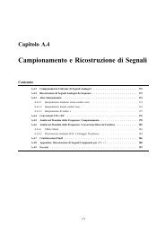
Contenuto
4.1 Riduzione della Ridondanza Temporale: Motocompensazione . . . . . . . . . . . . . . . . . . . 60
4.1.1 Motocompensazione in Avanti . . . . . . . . . . . . . . . . . . . . . . . . . . . . . . . . . 61
4.1.2 Motocompensazione Bidirezionale . . . . . . . . . . . . . . . . . . . . . . . . . . . . . . . 62
4.2 Successione di quadri con motocompensazione . . . . . . . . . . . . . . . . . . . . . . . . . . . 63
4.3 Gli Standard H.261 ed H.263 per la Compressione di Sequenze Video . . . . . . . . . . . . . . 64
4.3.1 Modi di codifica . . . . . . . . . . . . . . . . . . . . . . . . . . . . . . . . . . . . . . . . 66
4.3.2 Stima del moto e motocompensazione . . . . . . . . . . . . . . . . . . . . . . . . . . . . . 67
4.3.3 Codifica dei Vettori di Spostamento . . . . . . . . . . . . . . . . . . . . . . . . . . . . . . 67
4.3.4 Trasformazione DCT . . . . . . . . . . . . . . . . . . . . . . . . . . . . . . . . . . . . . . 67
4.3.5 Quantizzazione . . . . . . . . . . . . . . . . . . . . . . . . . . . . . . . . . . . . . . . . . 68
4.3.6 Codifica Entropica . . . . . . . . . . . . . . . . . . . . . . . . . . . . . . . . . . . . . . . 68
4.3.7 Controllo di Codifica . . . . . . . . . . . . . . . . . . . . . . . . . . . . . . . . . . . . . . 68
4.4 Standard H.262 (MPEG-2) . . . . . . . . . . . . . . . . . . . . . . . . . . . . . . . . . . . . . . 70
4.1 Riduzione della Ridondanza Temporale: Motocompensazione
Consideriamo una tipica sequenza video: essa è costituita dalla rapida successione di quadri (frames) ciascuno dei
quali è una immagine fissa.
Tali quadri si susseguono ad uno specifico frame-rate, tipicamente compreso fra 25 e 30 frames/s. Ciò implica
che la durata di presentazione di ogni singolo quadro sia compresa fra 33 e 40 ms/frame. Possiamo ragionevolmente
supporre che, in generale, due frame successivi presentino una alta correlazione fra loro: pensando infatti di riprendere
un soggetto in movimento, e.g. un presentatore del telegiornale, ci si rende immediatamente conto che tale soggetto
non potrà compiere movimenti troppo bruschi nel breve tempo occorrente fra due frame successivi. L’idea base da
cui partire è quindi che, in media, frame successivi siano molto simili fra loro.
La motocompensazione è, in essenza, un procedimento mediante il quale è possibile, in base a quanto detto sopra,
ottenere una riduzione della ridondanza temporale presente in una sequenza video. Considerando una coppia di quadri
adiacenti, infatti, se il quadro corrente è molto simile al quadro precedente, in fase di codifica dell’informazione
apportata dal quadro corrente potremo codificare solo la differenza, auspicabilmente piccola, fra i dati presenti nel
quadro corrente e quelli del quadro precedente, quest’ultimo detto di riferimento. Sarà inoltre necessario inviare
anche alcune informazioni relative al movimento intercorso fra i due quadri.
60

4.1. RIDUZIONE DELLA RIDONDANZA TEMPORALE: MOTOCOMPENSAZIONE 61
L’assunto di quadri molto correlati fra loro non è sempre corretto, basti pensare alla ripresa di un soggetto molto
veloce (una vettura di Formula 1, un pallone, etc.), o a caratteristiche tipiche delle pellicole cinematografiche, quali
i bruschi cambi di scena tipici del montaggio, o ancora ai cambi di scena dovuti ad un repentino cambiamento
dell’inquadratura. In tutti questi casi la motocompensazione non è in grado di operare in modo efficiente, e dunque
tali casi richiedono l’utlizzo di stratagemmi particolari, sempre che non sia possibile accettare il decadimento del
grado di compressione da essi causato. Peraltro, occorre sottolineare che, in generale, tali eventi sono ben tollerati e
solo in applicazioni critiche possono creare realmente problemi.
Entriamo ora più in dettaglio nel processo di motocompensazione. Come accadeva per la codifica per trasformate,
ciascun quadro viene suddiviso in blocchi da 8x8 pixel; inoltre, tali blocchi sono raggruppati a quattro a quattro nei
cosiddetti macroblocchi (MB) da 16x16 pixel.
4.1.1 Motocompensazione in Avanti
Tale caso prevede che ogni MB del quadro corrente sia confrontato (matched) con un sequenza bidimensionale di
64x64 pixel presenti nel quadro precedente, posizionati in genere nell’immediato intorno, cosiddetto Search Window,
del MB in esame; la sequenza che meglio rappresenta il MB in codifica è utilizzato come predittore di quest’ultimo
(best match), con ciò intendendo che il MB ottenuto dalla differenza fra i due è considerato come errore di predizione.
Sono inoltre calcolati i valori (in pixel) dello spostamento orizzontale e verticale del best-match MB rispetto a quello
corrente; tali informazioni costituiscono il cosiddetto Vettore di Spostamento (Motion Vector, MV).
Figura 4.1: Motocompensazione in Avanti

62 CAPITOLO 4. ELEMENTI DI CODIFICA VIDEO
Il calcolo del vettore spostamento si effettua come descritto nel seguito. Sia MBc i,j [0, 0] il pixel di riferimento
(in basso a sinistra), del macroblocco (i, j) del quadro corrente. I 64x64 pixel dell’intero macroblocco si ottengono
dalla sequenza bidimensionale MB (c)
i,j [n1,n2], 0 ≤ n1,n2 ≤ 15. Indicando con MB (p)
i,j [0, 0] il pixel di riferimento del
macroblocco (i, j) del quadro precedente, le componenti (dMV 1 ,dMV 2 ) del vettore spostamento sono determinate come
segue
(d MV
1 ,d MV
15X
15X
2 )=arg min
(d1,d2)∈SW
n1=0 n2=0
³
Φ MB (c)
i,j [n1,n2] − MB (p)
i,j [n1
´
− d1,n2 − d2]
(4.1.1)
avendo indicato con SW l’insieme dei pixel costituenti la Search Window, e con Φ(·) una opportuna funzione che
misura il costo associato alla differenza tra i macroblocchi del quadro corrente e del quadro di riferimento. Tipicamente
ΦSSD(·) =(·) 2 , costo che corrisponde alla minimizzazione della somma dei quadrati delle differenze (Sum of Squared
Differences, SSD), o ΦSAD(·) =|·|, costo che corrisponde alla minimizzazione della somma dei valori assoluti delle
differenze (Sum of Absolute Differences, SAD, oppure Mean Square Error, MSE).
La determinazione del vettore spostamento effettuata mediante la (4.1.1) è ottenuta mediante una ricerca esaustiva
sull’intera Search Window. Una Search Window utilizzata tipicamente nelle applicazioni, 15 ≤ d1,d2 ≤ 15, é
costituita da 31x31 pixel. Naturalmente, il vettore spostamento è vincolato in modo tale che tutti i pixel da esso
puntati siano entro l’area del quadro di riferimento.
Algoritmi di ricerca meno onerosi dal punto di vista computazionale, e.g. ricerca logaritmica, si applicano quando
è ragionevole assumere che la funzione da minimizzare nella (4.1.1) risulti convessa nell’intorno del suo minimo. In
generale, l’unica tecnica che assicura la determinazione del minimo della funzione di costo è la ricerca esaustiva;
tuttavia, il guadagno ottenuto in termini di tempi di calcolo da tecniche veloci spesso giustifica la loro adozione
poichè il prezzo da pagare in termini di predizione meno accurata è quasi sempre trascurabile.
4.1.2 Motocompensazione Bidirezionale
Figura 4.2: Motocompensazione Bidirezionale

4.2. SUCCESSIONE DI QUADRI CON MOTOCOMPENSAZIONE 63
Tale modalità costituisce una evoluzione della motocompensazione in avanti, in quanto consente di utilizzare sia un
quadro precedente che uno successivo a quello in codifica come predittori di quest’ultimo. Più in dettaglio, per ogni
MB in codifica è possibile utilizzare come riferimento o un best-matching MB appartenente al quadro precedente, o
un best-matching MB appartenente al quadro successivo, o la media fra tali due MB. In questo ultimo caso al MB
corrente competono due MV (MV1, MV2), ciascuno relativo ad uno dei due MB di riferimento.
Indicando con MB (f)
i,j [0, 0] il pixel di riferimento del macroblocco (i, j) del quadro successivo, le componenti
d MV1 =(d MV1
1
i.e.
,d MV1
2
) e d MV2 =(d MV2
1
d MV1 =argmin
d MV2 =argmin
,d MV2
2 ) dei due vettori spostamento sono determinante in modo indipendente,
15X
15X
d∈SW
n1=0 n2=0
15X
15X
d∈SW
n1=0 n2=0
³
Φ
³
Φ
MB (c)
i,j
MB (c)
i,j
[n] − MB(p)
i,j
[n] − MB(f)
i,j
´
[n − d]
´
[n − d]
(4.1.2)
La motocompensazione bidirezionale raggiunge più alti rapporti di compressione, ma ha una serie di svantaggi che ne
rendono non sempre conveniente l’impiego: richiede il doppio della memoria per immagazzinare i quadri, aumenta il
ritardo di codifica, porta un generale aumento della complessità del codificatore in quanto la fase di block-matching,
la più onerosa dal punto di vista computazionale di tutto il processo di codifica, deve essere eseguita due volte per
ogni MB.
4.2 Successione di quadri con motocompensazione
Con riferimento a un cosiddetto “Group of Pictures” (GOP), il primo quadro è sempre codificato senza motocompensazione
(INTRA), gli altri sono codificati con motocompensazione (INTER), con predizione in avanti (P), o
bidirezionale (B). I quadri di riferimento nella predizione bidirezionale possono essere I o P, ma non B. La dimensione
e la composizione di un GOP non sono fissati dai vari standard, dipendono piuttosto dalle esigenze maturate
nel corso della codifica. Un esempio è mostrato in Fig.4.3.
0 1 2 3 4 5 6 7 8
I
B B B P B B B
Figura 4.3: Un tipico GOP.
Con riferimento alla Fig.4.3, l’ordine con il quale il decoder riceverà i quadri sarà:
0 I , 4 P , 1 B , 2 B , 3 B , 8 I , 5 B , 6 B , 7 B
con conseguente aumento del ritardo complessivo di codifica.
I

64 CAPITOLO 4. ELEMENTI DI CODIFICA VIDEO
4.3 Gli Standard H.261 ed H.263 per la Compressione di Sequenze Video
Le raccomandazioni internazionali ITU riguardanti gli standard H.261 (Video Codec for Audiovisual Services at px64
kbit/s) e H.263 (Video Codec for Narrow Telecomunication Channels at < px64 kbit/s) specificano completamente
la struttura e il comportamento del codificatore, la sintassi e l’organizzazione del bitstream.
La sequenza video in ingresso è costituita da una sequenza di quadri YCBCR di luminanza/crominanza, 4.1 di
dimensioni CIF (288x360) o QCIF (144x180). 4.2 L’uso del CIF è opzionale, il QCIF è mandatorio.
Formato Dimensioni (Y )
CODEC
H.261 H.263
SQCIF 128x96 opzionale richiesto
QCIF 176x144 richiesto richiesto
CIF 352x288 opzionale opzionale
4CIF 704x576 non definito opzionale
16CIF 1408x1152 non definito opzionale
Tabella 4.1: Formati negli standard H.261 e H.263.
Il massimo frame-rate è 30000/1001 ' 29.97 fps, con la possibilità di saltare 1, 2 o 3 quadri.
Si noti che occorrono 36.45 Mbit/s per trasmettere, senza compressione, un video CIF alla massima velocità di
quadro, mentre per un video QCIF occorrono 9.115 Mbit/s .
Le componenti di crominanza sono sottocampionate in modalità 4:2:0, i.e. sottocampionate di un fattore 2 in
entrambe le direzioni, quattro pixel condividono la stessa crominanza (vedi Fig.4.4).
Figura 4.4: Sottocampionamento della crominanza 4:2:2 (sinistra) e 4:2:0 (destra). Il simbolo X rappresenta un generico
campione di luminanza, i due semi-quadrati rappresentano una coppia di campioni CRCB
luminanza (4:2:2), o da quattro campioni di luminanza (4:2:0).
condivisa da due campioni di
4.1 Dai coefficienti tricromatici del sistema di riferimento colorimentrico NTSC RN ,GN ,BN , la trasformazione in luminanza/crominanza si
ottiene nel modo seguente:
Y =0.299 · RN +0.587 · GN +0.114 · BN
CR = RN − Y
CB = BN − Y
4.2 Common Intermediate Format (CIF) e Quarter-CIF (QCIF), formati standard ITU.
;
RN = CR + Y
BN = CB + Y
GN = Y − 0.299 · RN − 0.114 · BN
0.587

4.3. GLI STANDARD H.261 ED H.263 PER LA COMPRESSIONE DI SEQUENZE VIDEO 65
Ogni quadro è diviso in gruppi di macroblocchi (GOB). A un macroblocco di 16x16 pixel di luminanza restano
associati due corrispondenti insiemi di 8x8 pixel di crominanza. In termini di blocchetti 8x8, un macroblocco consta
ad essere costituito da 6 blocchetti: 4 di luminanza, e i corrispondenti 2 di crominanza.
Tale struttura gerarchica è mostrata nella Fig.4.5.
Figura 4.5: Struttura gerarchica di Quadro
Il codificatore utilizza congiuntamente tecniche di predizione Inter-frame (per ridurre la ridondanza temporale mediante
motocompensazione) e tecniche di codifica a trasformata Intra-frame (per ridurre la ridondanza spaziale). La
struttura generale del codificatore è mostrata nella Fig.4.6.

66 CAPITOLO 4. ELEMENTI DI CODIFICA VIDEO
4.3.1 Modi di codifica
Figura 4.6: Schema semplificato del Codificatore H.263
I possibili modi di codifica sono essenzialmente due: INTER ed INTRA.
Il modo di codifica INTRA non prevede predizione interquadro. I frame codificati INTRA sono detti “frame-I”.
Il modo di codifica INTER, invece, prevede predizione interquadro con eventuale motocompensazione: in tale
modalità, per ciascun quadro, è codificato il cosiddetto “quadro errore di predizione”, ossia la differenza fra il quadro
corrente e quello predetto e motocompensato. I quadri codificati INTER con predizione in avanti sono detti “frame-P”.
Il modo di codifica può essere segnalato su base quadro (quadri I/P), o su base macroblocco nei quadri P.
Nello standard H.263 è possibile avere dei quadri codificati INTER con predizione bidirezionale (“frame-B”).
Un frame-B è sempre associato al successivo frame-P di riferimento in un cosiddetto frame-PB. Un esempio di GOP
con frame-FB é mostrato in Fig.4.7.
0 1 2 3 4
I
B
P B
PB PB
Figura 4.7: Un esempio di GOP nello standard H.263.
P

4.3. GLI STANDARD H.261 ED H.263 PER LA COMPRESSIONE DI SEQUENZE VIDEO 67
4.3.2 Stima del moto e motocompensazione
La valutazione del vettore spostamento si effettua solo su macroblocchi di luminanza. La motocompensazione sulla
crominanza si effettua utilizzando il vettore spostamento misurato dalla luminanza.
Nello standard H.261 la Search Window è limitata ai valori interi −15 ≤ d1,d2 ≤ 15.
Nello standard H.263, si considerano anche valori semi-interi, e.g. d1 =3.5,d2 =7.5, e la Search Window è
−16 ≤ d1,d2 ≤ 15.5. Per i valori semi-interi è necessario interpolare sul quadro precedente. Inoltre, è possibile
valutare il vettore spostamento su blocchetti 8x8.
4.3.3 Codifica dei Vettori di Spostamento
Nello standard H.263, il vettore di spostamento MV è codificato predittivamente, ossia è codificata la differenza
MVD fra tale vettore ed un opportuno vettore di spostamento “predittore” MVP, ottenuto come il valore mediano di
tre vettori opportunamente scelti fra quelli appartenenti a tre macroblocchi adiacenti, secondo quanto mostrato dalla
figura seguente. Le due componenti del vettore MVD sono poi codificate entropicamente utilizzando un codice a
lunghezza variabile specificato nello standard.
4.3.4 Trasformazione DCT
Figura 4.8: Vettori di Spostamento
La trasformazione DCT si applica ai blocchetti di 8x8 pixel, sia per i quadri codificati INTRA che per quelli codificati
INTER. Come nello standard JPEG, non é specificato un metodo specifico per calcolare la DCT.

68 CAPITOLO 4. ELEMENTI DI CODIFICA VIDEO
4.3.5 Quantizzazione
Per quanto riguarda il coefficiente DC, abbiamo sempre Q[0, 0] = 8. Per i restanti coefficienti (AC) abbiamo
Q[k1,k2] = 2·QP, con valori compresi fra 1 ≤ QP ≤ 31 (vedi Tab.4.2). Occorre sottolineare che il valore QP
è tenuto fissato per un intero macroblocco, i.e. non varia per blocchetti appartenenti allo stesso macroblocco. La
modalità di scelta non è specificata nello standard.
Naturalmente, il valore QP può variare a seconda del tipo di codifica (INTRA, INTER-P, INTER-B).
8 2·QP 2·QP 2·QP 2·QP 2·QP 2·QP 2·QP
2·QP 2·QP 2·QP 2·QP 2·QP 2·QP 2·QP 2·QP
2·QP 2·QP 2·QP 2·QP 2·QP 2·QP 2·QP 2·QP
2·QP 2·QP 2·QP 2·QP 2·QP 2·QP 2·QP 2·QP
2·QP 2·QP 2·QP 2·QP 2·QP 2·QP 2·QP 2·QP
2·QP 2·QP 2·QP 2·QP 2·QP 2·QP 2·QP 2·QP
2·QP 2·QP 2·QP 2·QP 2·QP 2·QP 2·QP 2·QP
2·QP 2·QP 2·QP 2·QP 2·QP 2·QP 2·QP 2·QP
Tabella 4.2: Tabelle dei passi di quantizzazione per quadri codificati INTRA nello standard H.263, con 1 ≤ QP ≤ 31. Per i
macroblocchi e quadri codificati INTER abbiamo ˙ X (DCT)
X
INTER [k1,k2] =round
(DCT)
INTER [k1,k2]
− QP/2
.
2·QP
4.3.6 Codifica Entropica
Dopo quantizzazione, come detto in precedenza, i blocchi si presentano come un insieme di valori intervallati da un
gran numero di zeri, e dunque ben si prestano ad una codifaca delle corse. Innanzitutto, i coefficienti quantizzati
vengono scanditi a “zig-zag”, come in JPEG.
La codifica delle corse si effettua mediante tre campi:
• LAST: indica se il coefficiente corrente sia o meno l’ultimo coefficiente diverso da zero nel blocco;
• RUN: il numero di zeri consecutivi che precedono il coefficiente da codificare;
• LEVEL : il valore non nullo del coefficiente da codificare.
I tre campi sono poi codificati mediante un codice di lunghezza variabile che però codicifica solo le terne più
frequentemente ricorrenti. Per le altre si ricorre a una opportuna sequenza cosiddetta di ESCAPE.
4.3.7 Controllo di Codifica
Essenzialmente, il controllo di codifica svolge due funzioni:
1. selezione del modo di codifica INTRA/INTER.;
2. assegnazione del parametro QP al quantizzatore.
Per comprendere la presenza del controllo di codifica, occorre sottolineare che il multiplexer a valle del codificatore
video deve erogare alla sua uscita un flusso di cifre binarie a velocità costante, sebbene al suo ingresso sia presente
un flusso con velocità non costante. A questo scopo provvede un’apposita memoria tampone (buffer), di dimensioni
limitate. Il controllo di codifica, quindi, dipende dallo stato di riempimento del buffer. Ad esempio, vicino alla

4.3. GLI STANDARD H.261 ED H.263 PER LA COMPRESSIONE DI SEQUENZE VIDEO 69
saturazione del buffer é necessario imporre una quantizzazione più dura (alto QP), evitare una codifica INTRA se
non arrivare a saltare il quadro.
In ogni caso, la selezione del modo di codifica avviene preventivamente confrontando il minimo della funzione di
costo della differanza tra macroblocco corrente e il suo best-match con opportune soglie. Ad esempio, con riferimento
al caso di motocompensazione in avanti (vedi la (4.1.1)), detto
C(d MV )=
15X
15X
n1=0 n2=0
³
Φ
MB (c)
i,j
£ MV
[n] − MB(p) i,j n − d ¤´
il costo associato alla scelta del vettore spostamento d MV , la selezione si effettua come illustrato in Fig.4.9.
0
SKIP INTER INTRA
t 1
Figura 4.9: Selezione del modo di codifica.
t 2
C d MV b g
Come già detto, si può decidere di non codificare affatto il quadro corrente, lasciando al decodificatore il semplice
compito di ricopiatura dal quadro di riferimento.

70 CAPITOLO 4. ELEMENTI DI CODIFICA VIDEO
4.4 Standard H.262 (MPEG-2)
Lo standard H.262 (MPEG-2) estende lo standard MPEG-14.3 per includere la codifica di sequenze video con qualità
televisiva, anche con la possibilità di interallacciamento di semiquadri.
Il paradigma della codifica è mutuato dallo standard H.261: blocchettizzazione, DCT, motocompensazione, e
codifica entropica.
Occorre notare che lo standard definisce solo il decodificatore e, conseguentemente, la sintassi del bit-stream dei
dati codificati. Naturalmente, il codificatore è costretto a generare un bit-stream sintatticamente corretto.
Un tipico GOP è illustrato in Fig.4.10, dove riconosciamo la presenza di quadri I,P, e B.
0 1 2 3 4 5 6 7 8
I
B B B P B B B
Figura 4.10: Un tipico GOP in MPEG-2.
I formati video sono specificati nei cosiddetti “livelli”, vedi Tab.4.3. 4.4
Livello Formato Massimo Rapporto d’Aspetto
Low 352x288 4/3
Main 720x576 (ITU-601) 4/3
High 1440 1440x1152 (HDTV) 4/3
High 1920x1152 (HDTV) 16/9
Tabella 4.3: Livelli MPEG-2.
Si noti che il rapporto d’aspetto può essere fissato indipendentemente dall’effettivo numero di pixel/linea e linee/quadro.
Altre informazioni sulla codifica sono collezionate nei cosiddetti “profili”, vedi Tab.4.4.
Profilo Caratteristiche
Simple come Main, senza frame B
Main Sottocampionamento 4:2:0, non scalabile
SNR Scalable Main con qualità scalabile
Spatial Scalable Main con dimensioni scalabili
4:2:2 Sottocampionamento 4:2:2 (produzione TV)
High Sottocampionamento 4:2:0, 4:2:2, pienamente scalabile
Multiview Stereo (un canale per occhio)
Tabella 4.4: Profili MPEG-2.
4.3 Moving Pictures Experts Group, ufficialmente ISO-IEC/JTC1/SC2/WG11.
4.4 Vedi anche http://www.dvb.org/dvb technology/dvb levels.htm.
I

4.4. STANDARD H.262 (MPEG-2) 71
Esempi di bit-rate ottenuti per coppia livello/profilo sono riportati in Tab.4.5.
Profilo/Livello Simple Main SNR
scalable
Low 352x288
4Mb/s
Main 720x576
15 Mb/s
720x576
15 Mb/s
High 1440 1440x1152
60 Mb/s
High 1920x1152
80 Mb/s
352x288
4 Mb/s
760x576
15 Mb/s
Tabella 4.5: Bit-rate in MPEG-2.
Spatial
scalable
720x576
(1440x1152)
60 Mb/s
4:2:2 High
720x576
50 Mb/s
1920x1152
300 Mb/s
352x288
(720x576)
20 Mb/s
720x576
(1440x1152)
80 Mb/s
960x576
(1920x1152)
100 Mb/s

Indice Analitico
Symbols
YCRCB .......................................49
C
CIF........................................... 64
codici......................................... 26
codificadisorgente.............................27 corse, codifica..................................28
D
DCT..........................................42
DFT...........................................38
E
entropia........................................25
G
GOP..........................................63
H
H.261.........................................64
H.262.........................................70
H.263.........................................64
H.263, codifica entropica........................68
H263, codifica dei vettori spostamento ...........67
H263, controllo di codifica ......................68
H263, GOB ....................................65
H263, modi di codifica .........................66
H263, quantizzazione . . . ........................68
Huffman, codifica..............................28
I
informazione, teoria.............................24
J
JPEG..........................................48
JPEG, codificaentropica........................53 JPEG, modalitàgerarchica......................58 JPEG, modalitàprogressiva......................56 JPEG, modalitàsequenziale.....................50 72
JPEG, quantizzazione...........................52
K
KLT...........................................36
L
livelliMPEG-2.................................70 M
motocompensazione.............................60
motocompensazionebidirezionale................62 motocompensazioneinavanti....................61 MPEG-2.......................................70
MSE..........................................62
P
profiliMPEG-2................................70 Q
QCIF..........................................64
QP............................................68
S
SAD..........................................62
SSD...........................................62
T
tasso-distorsione, funzione.......................30
Trasformata di Karhunen-Loeve .................36
TrasformataDiscretadelCoseno.................42 TrasformataDiscretadiFourier..................38 trasformateunitarie, codifica....................35