Elementi di meccanica dei materiali e metallurgia - Matematicamente.it

di Matteo Puzzle 

matematicare@hotmail.com 

per il gruppo 

http://it.groups.yahoo.com/group/softwarestrumentitecnologici/

“Elementi di meccanica dei materiali e metallurgia” di Matteo Puzzle – matematicare@hotmail.com 

L’autore è grato a chiunque voglia segnalare eventuali imprecisioni, riportate in 

questo documento, inoltre sono graditi commenti, suggerimenti e giudizi critici. 

Il presente documento può essere copiato, fotocopiato, riprodotto, a patto che non 

venga altera l’integrità, la proprietà dell’autore e il contenuto stesso. 

L’autore non potrà essere ritenuto responsabile per il contenuto e l'utilizzo del 

presente documento, declinandone ogni responsabilità. 

PROPRIETA’ Matteo Puzzle 

VERSIONE FILE 1.0 

DATA DI CREAZIONE 23 Settembre 2005 

ESTENSIONE FILE .pdf 

SITO http://www.matematicamente.it/ 

1


PARTE I: generalità sui materiali duttili e fragili .............................................................3 

Resistenza, duttilità ed energia di frattura ........................................................................3 

PARTE II: tensioni piane e tridimensionali (cerchi di mohr) ..........................................9 

Sforzi combinati: introduzione ..........................................................................................9 

Cerchio di mohr per uno stato di sforzo piano..................................................................9 

Cerchio di mohr per gli stati di deformazione piani.........................................................16 

Cerchio di mohr per uno stato di sforzo tridimensionale.................................................18 

Sollecitazione locale e quadrica indicatrice ...................................................................20 

PARTE III: criteri di snervamento ...................................................................................22 

Criterio del massimo sforzo di taglio (criterio di Tresca).................................................22 

Criterio della massima energia di distorsione (criterio di Von Mises) .............................23 

Confronto tra il criterio di Tresca e di Von mises............................................................30 

PARTE IV: introduzione ai processi di lavorazione meccanica...................................31 

Determinazione dei carichi per la trafilatura e la fucinatura da considerazioni tensionali: 

introduzione....................................................................................................................31 

Lavoro per variare la lunghezza di un elemento rettilineo ..............................................31 

Applicazione dell’equazione del lavoro: determinazione della massima possibile 

riduzione di una sezione in un unico passaggio .............................................................34 

Estrusione di una sbarra ................................................................................................35 

PARTE V: il processo di trafilatura ................................................................................36 

Processo di trafilatura: introduzione ...............................................................................36 

Sbarra cilindrica trafilata con una matrice conica ...........................................................37 

Legami sforzo – deformazione nel processo di trafilatura ..............................................42 

Determinazione della massima riduzione di un trefolo ...................................................46 

Esempio di trafilatura......................................................................................................47 

Osservazioni ..................................................................................................................50 

Elaborazioni grafiche......................................................................................................51 

Esempi di trafilatura di un filo .........................................................................................54 

Trafilatura di un tubo ......................................................................................................62 

PARTE VI: micrografie e macrografie ............................................................................65 

PARTE VII: appendice .....................................................................................................76 

Il patentamento ..............................................................................................................76 

Il microscopio .................................................................................................................78 

Microscopi ottici ..........................................................................................................78 

I microscopi elettronici ................................................................................................81 

BIBLIOGRAFIA.................................................................................................................84 

2


PARTE I: generalità sui materiali duttili e fragili 

Resistenza, duttilità ed energia di frattura 

I materiali strutturali vengono tradizionalmente catalogali, in base alle caratteristiche della 

curva tensione - deformazione σ ( ε ) , in due distinte categorie: materiali duttili e materiali 

fragili. Mentre i primi mostrano ampi tratti non lineari nel diagramma σ ( ε ) , prima di 

pervenire alla rottura, i secondi si rompono in modo improvviso, quando la risposta é 

ancora sostanzialmente elastica e lineare. Una seconda caratteristica che li distingue 

nettamente è il rapporto tra resistenza a trazione e resistenza a compressione. 

Mentre per i materiali duttili tale rapporto é vicino all'unità, per i materiali fragili esso si 

1 

presenta di molto inferiore (in alcuni casi, 10 − 2 e 10 − ). Le differenze di comportamento 

dipendono in gran parte dai meccanismi microscopici di danneggiamento e di frattura, che, 

nei vari materiali di impiego strutturale, si presentano notevolmente diversi. Nelle leghe 

metalliche, ad esempio, si verificano degli scorrimenti tra i piani atomici e cristallini, che 

danno luogo ad un comportamento di tipo plastico o duttile, con notevoli deformazioni 

permanenti. Nei calcestruzzi e nelle rocce, d'altra parte, le microfessure e gli scollamenti 

tra i componenti granulari e la matrice, possono estendersi e concorrere a formare una 

fessura macroscopica che separa improvvisamente in due parti l’elemento strutturale. 

Questo processo di fessurazione instabile produce un comportamento di tipo fragile. 

Peraltro, non é sempre evidente quale sia l'ambito microscopico in cui avvengono i 

meccanismi di danneggiamento. Tale ambito può presentare dimensioni assai diverse, in 

funzione della natura dei meccanismi e della eterogeneità del materiale. Nei cristalli il 

danneggiamento avviene a livello atomico, con le vacanze e le dislocazioni; nelle leghe 

metalliche le cricche si propagano a livello intergranulare o transgranulare; nei 

calcestruzzi, infine, le fessure si enucleano all'interfaccia tra gli inerti granulari e la matrice 

cementizia. Si comprende quindi come la scala del danneggiamento venga a dipendere 

dalla regolarità del solido e quindi dalla dimensione delle eterogeneità in esso presenti. 

Accanto ai materiali da costruzione tradizionali, si sono aggiunti oggi nuovi materiali, 

altamente eterogenei ed anisotropi, poiché rinforzati da fibre e composti da più lamine. Tali 

materiali, detti compositi, possono essere a matrice polimerica, metallica, ceramica o 

cementizia. In essi i meccanismi di danneggiamento sono essenzialmente due: lo 

sfilamento delle fibre e la delaminazione (cioè lo scollamento degli strati). 

La distinzione tra materiali duttili e materiali fragili non è sempre così netta nella pratica, 

anche perché la duttilità del materiale dipende dalla temperatura ambientale e anche dalla 

dimensione dell'elemento strutturale. 

Quest’ultima è la dipendenza concettualmente più ardua da intendere, poiché in questo 

modo la duttilità cessa di essere una proprietà del materiale per diventare una proprietà 

dell’intera struttura. 

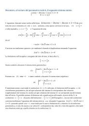
Si consideri una prova di trazione uniassiale eseguita su di un provino o campione di 

materiale duttile, ad esempio un acciaio (fig. 1.1). Il provino abbia l'usuale forma a 

clessidra, per evitare che la rottura avvenga nella zona terminale di ammorsamento alla 

macchina di prova. 

3


Figura 1.1 Figura 1.2 

Sia 0 A l'area della sezione trasversale iniziale del provino nella zona mediana ed l0 

la 

distanza iniziale tra due sensori incollali in due punti distinti della zona mediana. Tale 

distanza venga misurata da un dispositivo elettrico che collega i due punti. Si definisca la 

tensione nominale σ , come il rapporto tra la forza F trasmessa dalla macchina di prova 

e l'area iniziale A 0 . 

F 

σ = 

A 

Si trascurano cosi le contrazioni laterali elastiche ed, eventualmente, plastiche. 

Si definisca poi la dilatazione convenzionale ε , come il rapporto tra la variazione di 

distanza tra i due sensori l e la distanza iniziale : l 

∆ 0 

l−l0∆l ε = = 

l0 l0 

Tale dilatazione è quella media, relativamente al tratto sotto controllo. É molto probabile 

che, durante la prova, e specialmente in regime non lineare, la dilatazione non sia 

uniforme e quindi non sia puntualmente coincidente con quella media. 

Si riportino ora sul piano σ − ε tutte le coppie di punti registrati durante il processo di 

caricamento (figura 1.2). Tra i punti O e L il diagramma è lineare ed elastico. Da L in poi 

la risposta non è più lineare ed il materiale comincia a snervarsi. Scaricando il provino, si 

evidenziano delle deformazioni permanenti ε p . In questo modo parte dell'energia di 

' 

deformazione è restituita (triangolo ABA ), cioè quella relativa alla deformazione ε el , mentre 

' 

la restante è dissipata plasticamente (area OLAA ). Caricando nuovamente il provino, si 

' 

ripercorre elasticamente il tratto A A , parallelo al tratto OL . Giunti in A , il provino si snerva 

di nuovo ad una tensione σ > σ l . 

II materiale vergine, quindi, si snerva a livelli di tensione più bassi di quanto non faccia il 

materiale già precedentemente snervato. Tale fenomeno è detto incrudimento del 

materiale (in inglese: “hardening”). 

Continuando ad aumentare la forza applicata F , si riprende a percorrere il tratto non - 

lineare AU . In questa fase l’incremento di tensione per incremento unitario di dilatazione 

(ciò che si chiama solitamente rigidezza tangenziale) continua a diminuire, finché non si 

annulla nel punto U . Giunti nel punto U , se il processo di caricamento è pilotato dalla 

forza esterna F , il provino si rompe, poiché F non può ulteriormente aumentare. 

0 

4



D’altra parte, se il processo di caricamento é pilotato dalla variazione di distanza ∆ l (cioè, 

elettronicamente si impone a tale grandezza una rampa nel tempo), é possibile indagare 

sul comportamento del materiale al di là del punto di resistenza ultima U . Oltre il punto U , 

infatti, la rigidezza tangenziale diventa negativa e, ad incrementi positivi di spostamento 

∆l , corrispondono incrementi negativi della forza F . Ciò è dovuto al fenomeno della 

contrazione trasversale plastica o strizione (figura 1.3), per cui l'area A della sezione 

effettiva diventa notevolmente minore di A 0 , in una banda localizzata compresa tra i due 

sensori. Infine, raggiunto un punto S terminale, il provino cede di schianto, sebbene il 

processo di caricamento sia a deformazione controllata. 

Nel caso di alcune leghe metalliche, come gli acciai a basso tenore di carbonio, al limite di 

proporzionalità L segue uno snervamento improvviso, così che la dilatazione aumenta di 

una quantità finita sotto carico costante (figura 1.4). In questi casi è quindi facile 

individuare il valore della tensione di snervamento uniassiale σ p , essendo questa 

coincidente con il limite di proporzionalità σ l . Quando invece al limite di proporzionalità 

segue il tratto incrudente, è più difficile definire σ P . Si usa allora, per convenzione, quel 

valore della tensione la cui dilatazione permanente ε p allo scarico è pari al 0,2%. 

Mentre i materiali duttili presentano comportamenti simili a trazione c compressione, i 

materiali fragili mostrano comportamenti considerevolmente diversi. I calcestruzzi, ad 

esempio, sono duttili in compressione e fragili in trazione, e presentano una resistenza 

ultima a compressione che è circa di un ordine di grandezza maggiore di quella a trazione. 

Una prova di trazione su di un campione di calcestruzzo, se condotta pilotando il carico 

(come si suole dire, a carico controllato), mostra una risposta approssimativamente 

elastica e lineare e poi, all'improvviso, una brusca caduta del carico stesso, che 

corrisponde alla repentina formazione di una fessura. Tuttavia, le moderne tecniche 

elettroniche permettono oggi di pilotare la deformazione (input = deformazione ε , output 

= tensione σ ). 

Cosi facendo, si evidenzia la curva di risposta post - rottura del materiale cementizio 

(figura 1.5). Solo recentemente ci si è resi conto dell’esistenza di un esteso ramo di 

incrudimento negativo (in inglese: “softening”) e della possibilità di dissipare, da parte del 

materiale, una notevole quantità di energia per unità di volume. Tale energia è 

rappresentata dall'area sottesa dalla curva σ ( ε ) . 

5



Ancora più recentemente si è potuto dimostrare che l’energia in realtà non è dissipata 

uniformemente nell’unità di volume, bensì è dissipata su una banda localizzata, la quale 

diventa in seguito una fessura (lo stesso fenomeno avviene nei materiali duttili con la 

strizione). In altre parole, la dilatazione puntuale tra i due sensori di figura 1.1, non è una 

funzione costante. Al contrario, essa mostra un notevole picco in corrispondenza della 

fessura in via di formazione. Idealmente si può immaginare che la funzione ε sia una δ di 

Dirac, essendo la dilatazione infinita ove si verifica una discontinuità della funzione 

spostamento assiale. 

In conseguenza della localizzazione della deformazione ε , il ramo decrescente σ ( ε ) viene 

a dipendere dalla lunghezza l0 

della base di misura. Ciò che invece risulta essere una 

vera caratteristica del materiale è il diagramma σ ( w) 

, che rappresenta la tensione 

trasmessa attraverso la fessura, in funzione della apertura (o larghezza) della fessura 

stessa (figura 1.6). Tale legge di decadimento indica, naturalmente, un indebolimento 

dell'interazione all'aumentare della distanza w tra le facce (o superfici libere) della fessura. 

Quando w raggiunge il valore limite wc 

, l'interazione si spegne totalmente e la fessura 

diventa una sconnessione completa che divide in due parti distinte il provino. L'area 

sottesa dalla curva σ ( w) 

rappresenta l'energia dissipata sulla superficie unitaria di frattura. 

Essendo la legge coesiva σ ( w) 

una caratteristica del materiale, che dipende dalla struttura 

intima e dai meccanismi di danneggiamento del materiale stesso, anche l’energia di 

frattura ∑ risulta essere una proprietà intrinseca del materiale: 

∑=∫ 

wc 

0 

( ) 

σ wdw 

L'energia dissipata sulla superficie della fessura vale 0 A ∑⋅ essendo dimensionalmente ∑ 

un lavoro per unità di superficie e quindi una forza per unità di lunghezza, [ ][ ] 1 

F L − 

. 

Poiché, peraltro, si è supposto che la dissipazione energetica avvenga soltanto sulla 

superficie fessurata e non nel volume di materiale integro, l'energia dissipata globalmente 

nel volume A0⋅ l0 

è ancora pari a 0 A ∑⋅ (cioè rigorosamente valido in assenza di 

incrudimento positivo). 

Se si riportano allora le curve di risposta sul piano F − ∆ l, 

all'aumentare della lunghezza l0 

del provino, si ottengono tratti elastici a rigidezza calante e tratti “softening” a pendenza 

negativa crescente e, oltre un certo limite, a pendenza positiva (figura 1.7). L'area sottesa 

da ciascuna curva deve infatti essere costante e pari a ∑⋅ A . 

0 

6



Sul piano σ − ε (figura 1.8) la transizione appena descritta, è rappresentata da un unico 

tratto elastico lineare e da un ventaglio di rami “softening”, al variare della lunghezza l0 

. 

L'area sottesa, infatti, in questo caso varia con l 0 , essendo pari a ∑ / l0 

. 

Per l0 → 0 il ramo “softening” diventa orizzontale e rappresenta una risposta strutturale 

perfettamente plastica. D'altra parte, per l0 →∞ l'area compresa tra la curva σ ( ε ) e l’asse 

ε deve tendere a zero, e quindi il ramo “softening” tende a coincidere con il tratto elastico 

(figura 1.8). 

La pendenza positiva del ramo “softening” si può giustificare, oltre che, come si è visto, 

considerando l’energia dissipata, anche per derivazione analitica della funzione ε ( σ ) . 

Nella fase post-rottura si ha infatti (figura 1.9): 

∆l 

ε 

ε = = 

l l 

0 0 

el ⋅ l0+ w 

ove con ε el si è indicata la dilatazione specifica longitudinale 

nella zona integra: 

σ 

ε el = 

E 

Quindi si trae: 

σ w( 

σ ) 

e derivando rispetto a σ : 

ε = + 

E l 

dε1 1 dw 

= + ⋅ 

dσE l dσ 

Tale derivata, e quindi anche l’inversa 

Figura 1.9 

dσ 

, è maggiore di 

dε 

zero per: 

dw 

l0> E⋅ dσ 

Ne discende che si hanno tratti “softening” a pendenza positiva per: 

l 

0 

E 

> 

dw 

dσ 

cioè, quando la lunghezza del provino, o meglio la distanza l 0 tra i punti di cui si stima lo 

spostamento relativo, é superiore al rapporto tra modulo elastico e massimo modulo 

tangente della legge coesiva. Ciò è dovuto al fatto che, durante la fase di incrudimento 

negativo, la tensione σ diminuisce e, mentre il punto rappresentativo della zona fessurata 

max 

0 

0 

7


scende lungo la curva σ ( w) 

(figura 1.6),il punto rappresentativo della zona integra scende 

lungo la retta σ ( ε ) (figura 1.5) e descrive uno scaricamento elastico. Se la lunghezza l0 

è 

sufficientemente grande, la contrazione elastica prevale sulla dilatazione della zona 

fessurata, dando luogo al fenomeno precedentemente descritto. 

II “softening” a pendenza positiva rappresenta un fenomeno inquadrabile nell'ambito della 

Teoria delle Catastrofi. Se infatti il processo di carico è pilotato dalla dilatazione 

convenzionale e, o dall'allungamento ∆ l , una volta raggiunto il punto U (figura 1.7), si ha 

una caduta verticale del carico, sino ad incontrare il tratto “softening” inferiore che è a 

pendenza negativa. II tratto UQT viene così ignorato e diventa virtuale. Per rilevare 

sperimentalmente questo tratto, è necessario pilotare il processo di carico mediante 

l'apertura w della fessura, cosa che oggi la tecnica elettronica consente. L'instabilità sopra 

descritta, con termine anglosassono, é detta “snapback”. Tutti i materiali relativamente 

fragili (come il calcestruzzo, la ghisa, il vetro, il plexiglass,...), che possiedono un basso 

valore della energia di frattura ∑ , con le normali lunghezze l 0 dalla base di misura 

presentano una brusca caduta del carico quando il comportamento globale del campione 

è ancora elastico lineare. 

Concludendo queste premesse, è opportuno osservare come resistenza ed energia di 

frattura siano proprietà intrinseche del materiale, mentre la duttilità dipenda da un fattore 

strutturale come la lunghezza del campione. 

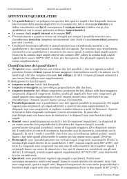
In figura 1.10 sono 

riportate provette 

proporzionali secondo il 

metodo di prova di 

trazione per i materiali 

metallici, a temperatura 

ambiente, norma UNI 

EN 10002/1. Secondo 

tale norma, la forma e la 

dimensione delle 

provette sono 

determinate dalla forma 

e dalle dimensioni dei 

prodotti da esaminare. 

La provetta si chiama 

proporzionale quando la 

lunghezza l0 

è uguale a 

5, 65 ⋅ S0 

oppure quando 

l 0 = 5⋅d 

se la sezione è 

tonda, di diametro d . 

Figura 1.10 

Inoltre, sono riportate in sezione due tipi di provette che si possono ricavare da fili, barre, 

profilati con diametro o lato ≥ 4mm oppure da lamiere con spessore ≥ 3mm . 

Inoltre, sulla superficie della provetta si delimita una lunghezza incidendo due tacche di 

riferimento distanti non meno di 20mm . Dopo aver determinato l’area della sezione iniziale 

e aver marcato la lunghezza iniziale, la provetta è posizionata con appropriati dispositivi 

nella macchina di prova in modo che il carico sia applicato il più assialmente possibile. 

8


PARTE II: tensioni piane e tridimensionali (cerchi di mohr) 

Sforzi combinati: introduzione 

Le prove meccaniche (di trazione, compressione, flessione e torsione) possono essere 

usate per determinare in quali condizioni un metallo snerva sotto l’azione di un semplice 

sforzo di compressione o taglio. 

Tutti i processi di lavorazione meccanica dei metalli (estrusione, laminazione, fucinatura e 

trafilatura) implicano l’applicazione di un sistema di sforzi che è più complesso rispetto alle 

metodologie utilizzate per l’analisi di queste stesse tensioni, ma, è possibile analizzare 

questi sforzi riferendoli ai criteri di snervamento, i quali indicano consentono di calcolare 

sotto quali livelli di sforzo si verifica scorrimento plastico. 

Una rappresentazione introdotta da Otto Mohr è molto utile a tal fine, specialmente negli 

stati di sforzo piano bidimensionali. 

Cerchio di mohr per uno stato di sforzo piano 

Dato un elemento prismatico, consideriamo la direzione principale dello sforzo ' 

x , 

∆S ' ' 

normale al piano inclinato (fig. 2.2 - superficie gialla), e lo sforzo di taglio τ x y parallelo 

alla superficie ∆S 

, come in figura: 


Le aree delle faccette dell’elementino misurano: 

∆ S = AA'⋅ AC 

AA'⋅ AB =∆S⋅ cosθBB 

'⋅ BC = ∆S⋅ sinθ 

' 

L’angolo θ è compreso tra gli assi x e x e , per costruzione, è anche l’angolo BAC . 

σ 

9


τ 

Gli sforzi σ ' 

' ' 

x e x y rappresentano le componenti associate allo stesso elemento dopo 

che questo è stato ruotato di un angolo θ attorno all’asse cartesiano z ; vedi figure 2.3 e 

2.4: 


Trattandosi di sforzi piani, quindi bidimensionali, ne consegue che: 

⎧ σ z = 0 

⎪ 

⎨τ 

zx = 0 

⎪ 

⎩τ 

zy = 0 

inoltre, è facilmente dimostrabile: 

⎧⎪ τxy = τ yx 

⎨ 

⎪⎩ τ x 'y'= τ y'x' Per calcolare lo sforzo normale σ ' e lo sforzo tangenziale τ ' ' esercitati sul piano generico 

x 

' 

∆S 

perpendicolare all’asse x (inclinato arbitrariamente di un angolo θ rispetto agli assi x 

' 

e y ) , si considera un elemento prismatico con le facce perpendicolari agli assi x e y e x . 

Avendo indicato l’area obliqua con ∆ S , le aree perpendicolari agli assi x e y , 

coerentemente all’angolo θ , si esprimono in funzione di quest’ultimo: 

∆S⋅ cosθ 

indica la faccia perpendicolare all’asse x 

∆S⋅ sinθ 

indica la faccia perpendicolare all’asse 

Poiché l’elemento prismatico è in equilibrio, utilizzando le componenti lungo gli assi ' 

x e 

' 

y , si scrivono le seguenti equazioni di equilibrio [2.1.1]: 

∑ F ' 

x σ ' 

x S σx ( S θ) θ τxy ( S θ) θ σ y ( S θ) θ τxy ( S θ) θ 

F ' τ ' ' S σ ( S θ) θ τ ( S θ) θ σ ( S θ) θ τ ( S θ) 

θ 

∑ 

y 

= 0 ⇒ ⋅∆ − ⋅ ∆ ⋅cos ⋅cos − ⋅ ∆ ⋅cos sin − ⋅ ∆ ⋅sin ⋅sin − ⋅ ∆ ⋅ sin cos = 0 

= 0 ⇒ ⋅∆ + ⋅ ∆ ⋅cos ⋅sin − ⋅ ∆ ⋅cos cos − ⋅ ∆ ⋅sin ⋅cos − ⋅ ∆ ⋅ sin sin = 0 

xy 

x xy y xy 

dividendo ambo i membri delle due equazioni di equilibrio con ∆ S , ed esplicitando σ ' 

dalla prima equazione e τ ' ' dalla seconda equazione di equilibrio, si ottiene: 

x y 

σ 

' 

x 

2 2 

τ =−( σ x −σ y) ⋅sinθ ⋅ cosθ + τxy ⋅( cos θ −sin 

θ) 

' ' 

x y 

= σ ⋅ θ + σ ⋅ θ + ⋅τ ⋅ θ ⋅ θ 

2 2 

x cos y sin 2 xysincos 

Ricordando le relazioni trigonometriche: 

⎧sin 

( 2⋅ θ ) = 2⋅sinθ⋅cosθ ⎪ 

2 2 

⎪cos( 

2⋅ θ ) = cos θ −sin 

θ 

⎪ 

⎨ 2 1+ cosθ 

cos θ = 

⎪ 2 

⎪ 

2 1−cosθ ⎪ sin θ = 

⎪⎩ 2 

y 

x y 

x 

[2.1.2] 

10


l’espressione [2.1.2] di σ ' diventa: 

σ ' 

x 

1+ cosθ 1−cosθ = σ x ⋅ + σ y ⋅ + τxy ⋅sin ( 2⋅ 

θ) 

2 2 

oppure: 

' ' 

x y 

σ ' 

x 

x 

σx + σ y σx −σ 

y 

= + ⋅cos( 2⋅ θ ) + τxy⋅sin( 2⋅ 

θ) 

[2.1.3] 

2 2 

Sostituendo le relazioni trigonometriche nell’espressione [2.1.2] dello sforzo tangenziale 

τ , si ottiene la relazione: 

Se ' ' 

x y 

τ ' ' 

xy 

τ ' ' 

xy 

σx −σ 

y 

=− ⋅sin ( 2⋅ θ ) + τxy ⋅cos( 2⋅ 

θ) 

[2.1.4] 

2 

τ si sceglie con il verso opposto a quanto indicato nella figura 2.2, la [2.1.4] diventa: 

σx −σ 

y 

= ⋅sin 2⋅ − xy ⋅cos2⋅ 2 

( θ ) τ ( θ) 

Per ottenere l’espressione dello sforzo normale σ ' è sufficiente sostituire ( θ + π /2) 

y 

all’angolo θ dell’equazione [2.1.3] di σ ' , quindi: 

σ ' 

y 


y 

= + ⋅cos 2⋅ + + xy ⋅sin2⋅ + 

2 2 

( θ π) τ ( θ π) 

essendo: 

cos( 2⋅ θ + π) =−cos( 2⋅θ) 

sin ( 2⋅ θ + π) =−sin ( 2⋅θ) 

l’equazione [2.1.5] di σ ' diventa: 

y 

σ ' 

y 

degli sforzi normali σ ' e σ ' si ottiene: 

x y 

x 

[2.1.5] 


y 

= − ⋅cos( 2⋅θ) −τxy⋅sin( 2⋅ 

θ) 

[2.1.6] 

2 2 

Si nota che, sommando membro a membro le equazioni [2.1.3] e [2.1.5] delle componenti 

σ ' + σ ' = σ x y x + σ y 

[2.1.7] 

Riassumendo, le espressioni delle componenti piane di sforzo sono: 

⎧ σx + σ y σx −σ 

y 

⎪σ 

' = + ⋅cos( 2⋅ θ ) + τxy ⋅sin( 2⋅θ) 

x 

⎪ 

2 2 

⎪ σx+ σ y σx −σ 

y 

⎨σ 

' = − ⋅cos( 2⋅θ) −τxy ⋅sin( 2⋅θ) 

y 

[2.1.8] 

⎪ 2 2 

⎪ σx −σ 

y 

⎪τ 

' '=− 

⋅sin ( 2⋅ θ) + τxy ⋅cos( 2⋅θ) 

x y 

⎪⎩ 2 

Si nota che esse rappresentano le equazioni parametriche di un cerchio; questo significa 

che, se si sceglie un sistema di assi ortogonali e si riporta un punto di ascissa σ ' e di 

x 

ordinata τ ' ' per ogni determinato valore del parametro θ , tutti i punti ottenuti in questo 

x y 

modo giaceranno su un cerchio. 

Nell’equazione [2.1.3] di 

σ ' 

x 

σ 

σx + σ y σx + σ y 

− = ⋅cos 2⋅ + xy ⋅sin2⋅ 2 2 

' 

x 

si porta al primo membro 

( θ ) τ ( θ) 

elevando al quadrato ambo i membri: 

2 2 

x + y x + σ y 

⎞ 

cos( 2 θ) τ xy sin ( 2 θ) 

⎛ σ σ ⎞ ⎛σ 

⎜σ'− x ⎟ = ⎜ ⋅ ⋅ + ⋅ ⋅ 

⎝ 2 ⎠ ⎝ 2 

⎟ 

⎠ 

σ x + σ y 

2 

, quindi diventa: 

11


elevando al quadrato ambo i membri anche nell’equazione dello sforzo tangenziale [2.1.4]: 

τ 

2 

' ' 

x y 

⎛ σx + σ y 

⎞ 

= ⎜− ⋅sin ( 2⋅ θ) + τxy ⋅cos( 2⋅θ) 

⎟ 

⎝ 2 

⎠ 

Ora, sommando membro a membro si ottiene: 

2 

2 2 2 

⎛ σx + σ y ⎞ 2 ⎛σx + σ y ⎞ ⎛ σx + σ y 

⎞ 

⎜σ' − τ ' ' 

cos( 2 θ) τxy sin ( 2 θ) sin ( 2 θ) τxy cos( 2 θ) 

x ⎟ + = 

xy ⎜ ⋅ ⋅ + ⋅ ⋅ ⎟ + ⎜− ⋅ ⋅ + ⋅ ⋅ ⎟ 

⎝ 2 ⎠ ⎝ 2 ⎠ ⎝ 2 

⎠ 

2 2 

⎧⎛σx 

+ σ y ⎞ σx + σ ⎛ 

y ⎛σx + σ y ⎞ ⎞ 

2 2 2 

⎪⎜ 

⋅cos( 2⋅ θ) + τxy ⋅sin ( 2⋅ θ) ⎟ = ⋅τxy⋅sin ( 4⋅ θ) + ⎜⎜ ⎟ −τ ⎟ xy ⋅cos( 2⋅ 

θ) + τxy 

⎪ 2 2 ⎜ 2 ⎟ 

⎪⎝ 

⎠ ⎝⎝ ⎠ ⎠ 

⎨ 

2 2 

2 

⎪⎛ σx + σ y 

⎞ σx + σ ⎛ 

y ⎛σx + σ y ⎞ ⎞ 

2 2 ⎛σx + σ y ⎞ 

⎪⎜− ⋅sin ( 2⋅ θ) + τxy 

⋅ cos( 

2⋅ θ) ⎟ =− ⋅τxy ⋅sin( 4⋅θ) −⎜⎜ ⎟ −τ ⎟ xy ⋅cos ( 2⋅ 

θ) 

+ ⎜ ⎟ 

⎪⎝ 2 

⎠ 2 ⎜⎝ 2 ⎠ ⎟ 

⎩ 

⎝ ⎠ 

⎝ 2 ⎠ 

la somma del secondo membro dell’equazione, diventa: 

σx + σ ⎛ 

y ⎛σx + σ y ⎞ ⎞ σ 2 2 2 x + σ ⎛ 

y ⎛σx + σ y ⎞ ⎞ 

2 2 ⎛σx + σ y ⎞ 

⋅τxy ⋅sin ( 4⋅ θ) + ⎜⎜ ⎟ −τ ⎟ xy ⋅cos( 2⋅ θ) + τ xy − ⋅τxy ⋅sin ( 4⋅θ) −⎜⎜ ⎟ −τ ⎟ xy ⋅cos( 2⋅ 

θ) 

+ ⎜ ⎟ 

2 ⎜⎝ 2 ⎠ ⎟ 2 ⎜⎝ 2 ⎠ ⎟ 

⎝ ⎠ ⎝ ⎠ 

⎝ 2 ⎠ 

in cui si elidono i termini contenenti il parametro θ : 

σx + σ y 

τxy θ 

2 

2 

⎛ ⎞ 

⎛σ + σ ⎞ 

⎜ ⎟ xy 

⎜⎝ 2 ⎠ ⎟ 

⎝ ⎠ 

2 2 2 

σ + σ 

τxy θ 

2 

x y 2 2 

2 x y 

x y 2 2 

⋅ ⋅sin ( 4⋅ 

) + ⎜ −τ ⎟⋅cos 

( 2⋅θ) 

+ τ − ⋅ ⋅sin ( 4⋅ 

) −⎜ −τ ⎟⋅cos 

( 2⋅θ) 

con i termini rimanenti si ottiene l’equazione: 

Definendo: 

σ x + σ y 

σ med = 

2 

2 

xy 

2 2 

σx + σ y σ 

2 2 x + σ y 

' − + ' ' = τ 

x x y xy + 

⎛ ⎞ ⎛ 

⎜σ ⎟ τ ⎜ 

⎝ 2 ⎠ ⎝ 2 

R = 

⎛σx + σ y ⎞ 

⎜ ⎟ 

⎝ 2 ⎠ 

2 

+ τ xy 

l’equazione [2.1.9] si riscrive nella forma: 

( med ) 

2 

2 2 

' τ ' R 

x x y 

σ − + ' 

⎞ 

⎟ 

⎠ 

2 

⎛ ⎞ 

⎛σ + σ ⎞ 

⎜ ⎟ xy 

⎜⎝ 2 ⎠ ⎟ 

⎝ ⎠ 

⎛σx + σ y ⎞ 

+ ⎜ ⎟ 

⎝ 2 ⎠ 

2 

[2.1.9] 

[2.1.10] 

σ = [2.1.11] 

la quale rappresenta l’equazione di un cerchio di raggio R centrato nel punto C di ascissa 

σ med e ordinata 0 (fig. 2.5). 

Nella figura 2.5, i due punti A e B in cui il cerchio di 

Mohr (dal nome dell’ingegnere tedesco Otto Mohr 

1835-1918 che per primo lo scoprì) interseca l’asse 

orizzontale, sono di particolare interesse: il punto A 

corrisponde al massimo valore dello sforzo normale 

σ ' 

x , mentre il punto B corrisponde al suo valore 

minimo. Inoltre entrambi i punti corrispondono a un 

valore nullo dello sforzo tangenziale τ ' ' 

x y . 

Così i valori θ p del parametro θ che corrispondono ai 

punti A e B possono essere ottenuti imponendo 

τ ' '= 

0 xy nell’equazione [2.1.4], oppure differenziando 

σ ' nell’equazione [2.1.3] e imponendo la derivata: 

x 

dσ 

' 

x 

0 

dθ 

Figura 2.5 

= 

12


Ora si svilupperanno entrambi i metodi per il calcolo di θ p . 

⎧τ 

' '= 

0 

x y 

⎪ 

⎨ σx+ σ y 

⎪τ 

' '=− 

⋅sin 2⋅ + τ xy ⋅cos 2⋅ 

xy ⎩ 2 

( θ ) ( θ ) 

quindi: 

σx + σ y 2⋅τ 1 ⎛ xy τ ⎞ 

−1 xy 

− ⋅sin( 2⋅ θ) + τxy ⋅cos( 2⋅ θ) = 0 ⇒ tan ( 2⋅ θp) = ⇒ θp= 

⋅tan ⎜ ⎟ 

2 σ x −σ y 2 ⎜σ ⎟ 

⎝ x −σ 

y ⎠ 

oppure: 

d ' 

2 τ x 1 ⎛ xy τ ⎞ 

−1 xy 

0 ( σx σ y) sin ( 2 θ) 2 τxy cos ( 2 θ) 0 tan ( 2 θp) 

θ p tan 

dθ 

σx σ y 2 σx σ y 

⋅ 

σ 

= ⇒− − ⋅ ⋅ + ⋅ ⋅ ⋅ = ⇒ ⋅ = ⇒ = ⋅ ⎜ 

⎟ 

− − ⎟ 

⎝ ⎠ 

L’equazione: 

2⋅τ 

xy 

tan ( 2⋅ 

θ p ) = 

[2.1.12] 

σ −σ 

x y 

definisce due valori 2 ⋅ θ p che differiscono di π radianti e dunque due valori θ p che 

differiscono di π /2 radianti. 

Poiché i due valori θ p definiti dall’equazione [2.1.12] sono stati ottenuti imponendo τ ' '= 

0 , 

è chiaro che sui piani principali non vengono esercitati sforzi tangenziali. 

Nella rappresentazione grafica del cerchio di Mohr (figura 2.5) si osserva: 

σ = σ + R 

max 

min 

med 

σ = σ −R 

med 

Sostituendo le espressioni [2.1.10] nell’equazioni [2.1.13]: 

⎧ σx + σ y 

⎪σ 

med = 

⎪ 

2 

⎪ 

2 

⎪ ⎛σx + σ y ⎞ 2 

⎨R = ⎜ ⎟ + τ xy 

⎪ ⎝ 2 ⎠ 

⎪ 

⎪ 

σmax = σmed 

+ R 

⎪ ⎩σmin 

= σmed 

−R 

si ottiene: 

σx + σ y ⎛σx + σ y ⎞ 

σ max,min = ± ⎜ ⎟ + τ 

2 ⎝ 2 ⎠ 

2 

2 

xy 

xy 

[2.1.13] 

[2.1.14] 

Il raggio del cerchio di Mohr (figura 2.5) essendo pari alla differenza tra σ max e σ min , si 

scrive: 

1 

τmax = ⋅( σmax − σmin 

) 

2 

[2.1.15] 

dτ 

' ' 

xy 

Ora, imponendo la condizione 

dθ 

0 , si ottiene: 

= 

dτ 

' ' 

xy 

dθ 

σx + σ y 2⋅τ 1 ⎛ xy τ ⎞ 

−1 xy 

= 0 ⇒ ⋅cos( 2⋅ θ) + τxy ⋅sin ( 2⋅ θ) = 0 ⇒ tan ( 2⋅ θs) = ⇒ θs= 

⋅tan ⎜ ⎟ 

2 σx −σ y 2 ⎜σx −σ 

⎟ 

⎝ y ⎠ 

2⋅τ 

xy 

tan ( 2⋅ 

θs 

) = 

σ −σ 

[2.1.16] 

x y 

questo risultato, definisce due valori 2⋅ θs 

che differiscono di π radianti (180°) e dunque 

due valori θ s che differiscono di π /2 radianti (90°). 

13


Osservando dalla figura 2.5 che il massimo valore dello sforzo tangenziale è pari al raggio 

R del cerchio, e richiamando la seconda equazione della [2.1.10], si scrive: 

2 

⎛σx −σ 

y ⎞ 2 

τ max = ⎜ ⎟ + τ xy 

[2.1.17] 

⎝ 2 ⎠ 

Paragonando θ p della [2.1.12] e il valore di θ s della [2.1.16] si nota che gli angoli ( 2⋅ θ p ) e 

(2 ⋅ θs 

) differiscono di 90° e quindi gli angoli θ p e θ s differiscono di 45° (fig. 2.7). 

Si conclude dunque, che i piani di massimo sforzo tangenziale sono inclinati di 45° ( π /4 

radianti) rispetto ai piani principali. 

Ora si possono ricavare gli sforzi normali, 

cioè σ ' e σ ' , e lo sforzo tangenziale τ ' ' 

x 

y 

esercitati in corrispondenza del piano di 

massimo sforzo tangenziale inclinato di 

45° rispetto ai piani principali (figura 2.6 e 

micrografia 6.30 della parte VI): 

⎧ σx+ σ y 

⎪σ 

' ( max) 

= + τ 

x 

⎪ 

2 

π 

σx + σ 

⎪ 

y 

θ = = 45 ⇒⎨σ'( max) 

= −τ 

y 

4 ⎪ 

2 

⎪ 

σx −σ 

y 

⎪τ 

' '( 

max) 

=− 

xy 

⎪⎩ 

2 

Nel caso di trazione semplice: 

⎧ σ x 

σ ' ( max) 

= 

xy 

xy 

x y 

Figura 2.6 

⎪ x 2 

⎪ 

⎧⎪σy= 0 ⎪ σ x 

⎨ ⇒ ⎨σ'( 

max) 

= 

y 

⎪⎩ τ xy = 0 ⎪ 

2 

⎪ 

σ x 

⎪τ 

' '( 

max) 

=− 

xy 

⎩ 

2 

Quindi, se in un provino di sezione A si applica una forza di trazione F , questa genera, su 

un piano cristallino inclinato di un angolo θ rispetto ad A , una componente di taglio 

F ⋅ sinθ 

, che agisce sull’area A /cosθ 

, provocando uno sforzo di taglio: 

τ 

F 

A 

sinθ cosθ σ sinθ cos 

= ⋅ ⋅ = ⋅ ⋅ θ [2.1.18] 

Il cui valore massimo è raggiunto nel piano cristallino inclinato di 45°, per cui: 

F ⎛π⎞ ⎛π ⎞ F 1 σ 

τ = ⋅sin ⎜ ⎟⋅ cos⎜ 

⎟= 

⋅ = 

A ⎝ 4⎠ ⎝ 4⎠ A 2 2 

[2.1.19] 

14


Quindi, i piani che si muovono per primi sotto 

l’azione della forza F dovrebbero essere quelli 

orientati a 45° rispetto alla direzione dello 

sforzo. Dato però che le dislocazioni si 

muovono più facilmente sui piani e nelle 

direzioni di massima densità atomica, la 

deformazione inizierà su quelli, tra i piani favoriti 

cristallograficamente, il cui orientamento è più 

vicino ai 45° rispetto alla direzione dell’asse di 

sollecitazione. Lo scorrimento successivo di 

piani diversamente orientati provoca a livello 

microscopico una deformazione a zig zag , 

mediamente orientata intorno ai 45° rispetto allo 

sforzo, e spiega il progredire della 

deformazione con l’aumento del carico, 

evidenziata dalla curva σ / ε . 

Qualunque sia la possibilità di movimento di Figura 2.7 

una dislocazione (in campo elastico) essa non può superare il bordo del grano, per cui la 

deformabilità plastica e il carico di snervamento di un metallo sono condizionati anche 

dalle dimensioni del grano cristallino: a parità di altre condizioni i metalli a grano fine 

hanno pertanto carico di snervamento maggiore rispetto a quelli a grano grosso. 

Il meccanismo sopra descritto è responsabile del diverso comportamento alla 

deformazione plastica dei materiali metallici, ceramici e polimerici. I metalli sono 

intrinsecamente malleabili in quanto la mancanza di direzionalità del legame metallico 

minimizza il disturbo alla configurazione elettronica del legame quando gli atomi si 

spostano lungo un piano di scorrimento. Ben diverso è invece il caso dei ceramici, in 

quanto questi materiali sono dotati di legami ionici e/o covalenti. Nel caso del legame 

covalente gli elettroni sono localizzati in corrispondenza del legame tra gli atomi rendendo 

particolarmente difficile l’allontanamento definitivo degli stessi. Nel caso invece di legame 

ionico la deformazione risulta fortemente ostacolata in certe direzioni, per l’azione di 

repulsione di ioni dello stesso segno che verrebbero ad affacciarsi gli uni agli altri per 

spostamento del reticolo, e favorita in quelle direzioni che mantengono la posizione 

relativa tra ioni di segno opposto. Ancora diverso è il caso di materiali polimerici, per i quali 

la deformazione non è legata al movimento di dislocazioni, ma è condizionata dalla 

presenza di lunghe catene, lineari e/o ramificate, dal modo in cui sono legate tra loro e 

dalla temperatura. In ogni caso la deformazione plastica comporta lo scorrimento e 

l’allineamento irreversibile di segmenti di catene. 

15


Cerchio di mohr per gli stati di deformazione piani 

Riscrivendo le espressioni delle componenti piane di sforzo mostrate nella [2.1.8] rispetto 

alle deformazioni si ottiene: 

⎧ εx + εy εx −εy 

⎪ε 

' = + ⋅cos( 2⋅ θ) + γ xy ⋅sin( 2⋅θ) 

x 

⎪ 

2 2 

⎪ εx + εy εx −εy 

⎨ ε ' = − ⋅cos( 2⋅θ) −γ xy ⋅sin( 2⋅θ) 

y 

[2.2.1] 

⎪ 2 2 

⎪ γ ' '=−( 

εx −εy) ⋅sin ( 2⋅ θ) + γ xy ⋅cos( 2⋅θ) 

xy ⎪ 

⎪⎩ 

Il cerchio di Mohr, per gli stati di deformazione, si esprime: 

2 2 

2 

' ' 

x + ⎛γ⎞ y xy 

xy x − y 

⎛ ε ε ⎞ 

⎜ε'− x ⎟ 

⎝ 2 ⎠ 

Definendo: 

+ ⎜ 

⎝ 2 

⎟ 

⎠ 

⎛γ = ⎜ 

⎝ 2 

⎞ 

⎟ 

⎠ 

2 

⎛ε 

ε ⎞ 

+ ⎜ ⎟ 

⎝ 2 ⎠ 

[2.2.2] 

ε x + ε y 

ε med = 

2 

2 2 

⎛γ xy ⎞ ⎛εx−εy⎞ R = ⎜ ⎟ + ⎜ ⎟ 

⎝ 2 ⎠ ⎝ 2 ⎠ 

l’equazione [2.2.2] si riscrive nella forma: 

[2.2.3] 

2 

2 γ ' ' 

xy 

( ε ' − ε med ) + x 

4 

2 

= R 

[2.2.4] 

In figura 2.8, i punti A e B in cui cerchio di Mohr interseca l’asse orizzontale corrispondono 

alle deformazioni principali ε max e ε min , da cui: 

εmax = εmed 

+ R 

εmin = εmed 

−R 

Si conclude: 

[2.2.5] 

ε 

max,min 

2 2 

x + y ⎛ xy ⎞ ⎛ x − y ⎞ 

ε ε γ ε ε 

= ± ⎜ ⎟ + ⎜ ⎟ 

2 ⎝ 2 ⎠ ⎝ 2 ⎠ 

Imponendo ' ' 

xy 

γ = 0 

, cioè: 

[2.2.6] 

⎧γ 

' '= 

0 

⎪ x y 

⎨ 

⎪⎩ 

γ ' '=− 

x y sin 2 xy cos 2 ) 

x y ( ε −ε ) ⋅ ( ⋅ θ) + γ ⋅ ( ⋅θ 

si ricava l’equazione: 

[2.2.7] 

( εx −εy) ⋅sin ( 2⋅θ) −γ xy ⋅cos( 2⋅ θ) 

= 0 

[2.2.8] 

2⋅ θ p : 

che fornisce il valore dell’angolo ( ) 

2⋅ 

γ xy 

tan ( 2⋅ 

θ p ) = 

ε −ε 

x y 

[2.2.9] 

Il valore massimo dello scorrimento angolare nel piano è dato (richiamando il valore del 

raggio R della [2.2.2]): 

( ) 2 

γ = ⋅ = ε − ε + γ 

[2.2.10] 

2 

max 2 R x y xy 

16


Le deformazioni provocate in 

corrispondenza del piano di massimo 

sforzo tangenziale inclinato di 45° rispetto 

ai piani principali, si esprimono: 

⎧ εx + εy 

⎪ε 

' = + γ 

x 

xy 

⎪ 

2 

π ⎪ εx + εy 

θ = ⇒ ⎨ε 

' = −γ 

y 

xy 

4 ⎪ 2 

' ' 

x y 

( ε x ε y ) 

⎪ γ =− − 

⎪ 

⎪⎩ 

Figura 2.8 

17


Cerchio di mohr per uno stato di sforzo tridimensionale 

In un sistema tridimensionale ci sono tre facce di un elementino perpendicolari tra loro e 

gli sforzi tangenziali sono nulli. 

Gli sforzi principali sono σ 1 , σ 2 e σ 3 in cui sussiste la relazione: 

σ1 > σ2 > σ3 

Considerando il generico elementino tetraedico (fig. 2.9) e imponendo che la risultante 

delle forze sia nulla, in quanto l’elementino è in equilibrio, si ottiene l’equazione: 

F = 0 

∑ 

n 


n ⋅∆A−( x ⋅∆A⋅nx) ⋅nx−( xy ⋅∆A⋅nx) ⋅ny−( xz ⋅∆A⋅nx) ⋅nz−( yx ⋅∆A⋅ny) ⋅nx 

( σ y Any) ny ( τ yx Any) nz ( τzx Anz) nx ( τzy Anz) ny ( σz 

Anz) nz 

0 

σ σ τ τ τ 

− ⋅∆ ⋅ ⋅ − ⋅∆ ⋅ ⋅ − ⋅∆ ⋅ ⋅ − ⋅∆ ⋅ ⋅ − ⋅∆ ⋅ ⋅ = 

dividendo per l’area ∆ A : 

2 2 2 

σn = σx ⋅ nx + σ y ⋅ ny + σz ⋅ nz + 2⋅τxy ⋅nx⋅ ny + 2⋅τ yz ⋅ny ⋅ nz + 2⋅τzx⋅nz 

⋅ x n 

Si noti che l’espressione ottenuta per lo sforzo normale σ n è una forma quadratica in n x , 

ny e n z . Ne consegue che si potrebbero scegliere gli assi coordinati in modo che il 

secondo membro dell’equazione di sopra, si riduca alla somma di tre termini contenenti i 

quadrati dei coseni direttori. Indicando gli sforzi normali, degli assi coordinati 

corrispondenti, con σ 1 , σ 2 e σ 3 , e i coseni direttori con, n1 , 2 e , si scrive: 

n 3 n 

2 2 

2 

σ = σ ⋅ + σ ⋅ + σ ⋅n 

n n n 

1 1 2 2 3 3 


Da ciò che si evince in fig. 2.10, si può scrivere: 

2 2 2 2 2 2 2 2 

σn + τn = σ1 ⋅ n1 + σ2 ⋅ n2 

+ σ3 

⋅n 3 

Ricordando dalla trigonometria che: 

n n n 

2 2 2 

1 + 2 + 3 = 1 

Risolvendo rispetto ai coseni direttori si ottiene: 

2 

⎧ 2 ( σ n −σ2) ⋅( σn −σ3) ⋅τn 

⎪n1 

= 

⎪ ( σ1−σ2) ⋅( σ1−σ3) ⎪ 

2 

⎪ 2 ( σ n −σ1) ⋅( σn −σ3) ⋅τn 

⎨n2 

= 

⎪ ( σ2 −σ1) ⋅( σ2 −σ3) 

⎪ 

2 

2 ( σ n −σ2) ⋅( σn −σ1) ⋅τ 

⎪ n 

n3 

= 

⎪ ( σ −σ ) ⋅( σ −σ 

) 

⎩ 

3 1 3 2 

18


Concludendo, ci sono di conseguenza tre cerchi nel diagramma σ n e τ n riferiti ai tre sforzi 

principali (fig. 2.11), di equazione: 

2 2 

σ2 + σ3 2 σ2 −σ3 

n − + n = 

⎛ ⎞ ⎛ 

⎜σ τ 

2 

⎟ ⎜ 

⎝ ⎠ ⎝ 2 

2 2 

σ1 + σ2 2 σ1 −σ2 

n − + n = 

⎛ ⎞ ⎛ 

⎜σ τ 

2 

⎟ ⎜ 

⎝ ⎠ ⎝ 2 

2 2 

σ1 + σ3 2 σ1 −σ3 

n − + n = 

⎛ ⎞ ⎛ 

⎜σ τ 

2 

⎟ ⎜ 

⎝ ⎠ ⎝ 2 

⎞ 

⎟ 

⎠ 

⎞ 

⎟ 

⎠ 

⎞ 

⎟ 

⎠ 

Figura 2.11 

19


Sollecitazione locale e quadrica indicatrice 

Scrivendo l’espressione dello sforzo nelle tre direzioni principali di un elementino 

sollecitato tridimensionalmente, si osserva che esiste in P una faccetta in cui il suo sforzo 

è pn n σ = ⋅ (fig. 2.12), da cui per l’equilibrio di Cauchy si ottiene: 

⎧σ ⋅ nx = σx⋅ nx + τxy⋅ ny 

+ τxz⋅nz 

⎪ 

⎨σ 

⋅ ny = τxy⋅ nx + σ y⋅ ny 

+ τzy⋅nz 

⎪ 

⎩σ 

⋅ nz = τxz⋅ nx + τzy⋅ ny 

+ σz⋅nz 

Le direzioni principali , e acquistano il 

n 

nx y n z 

significato di autovettori del sistema lineare 

omogeneo con i corrispondenti autovalori σ : 

⎡σx −σ ⎢ 

⎢ τxy ⎢ 

⎣ τxz τxy σ y −σ τzy τ ⎤ xz ⎡nx⎤ ⎡0⎤ ⎥ 

τ 

⎢ 

zy n 

⎥ ⎢ 

y 0 

⎥ 

⎥⋅ ⎢ ⎥ 

= 

⎢ ⎥ 

σz−σ⎥ ⎦ 

⎢⎣n⎥ ⎢ z ⎦ ⎣0⎥⎦ Figura 2.12 

Per determinare l’equazione caratteristica dello stato di sforzo si impone nullo il 

determinante della matrice dei coefficienti: 

σ −σ 

τ τ 

x xy xz 

τ σ − σ τ = 0 

xy y zy 

τ τ σ −σ 

xz zy z 

Posto: 

T = σ + σ + σ 

T 

T 

I x y z 

= σ ⋅ σ + σ ⋅ σ + σ ⋅σ −τ −τ −τ 

2 2 2 

II y z z x x y yz zx xy 

σ τ τ 

x xy xz 

III = τ xy σ y τzy 2 2 2 

= σx⋅σ y ⋅σz−σx⋅τ yz −σ y ⋅τzx−σz⋅ τxy+ 2⋅τ 

yz ⋅τzx ⋅τ 

yx 

τ τ σ 

xz zy z 

in cui TI 

rappresenta l’invariante lineare di 

primo ordine (raccoglie tutti i termini di primo 

grado), TII 

rappresenta l’invariante 

quadratico di secondo ordine (raccoglie tutti i 

termini di secondo grado) ed infine TIII 

rappresenta l’invariante cubico di terzo 

ordine (raccoglie tutti i termini di terzo grado). 

Dal calcolo del determinante si ottiene: 

3 2 

σ −TI ⋅ σ + TII ⋅σ − TIII 

= 0 

che esprime l’equazione caratteristica dello 

stato di sforzo. L’interpretazione geometrica 

dello sforzo locale è una quadrica 

denominata ellissoide di Lamé (fig. 2.13). 

Figura 2.13 

20


Le tra radici σ I , σ II e σ III della equazione 

caratteristica dello stato di sforzo, sono 

indipendenti dal riferimento adottato e sono 

peraltro completamente determinate quando 

si conoscono i tre coefficienti; anche questi 

sono dunque indipendenti dal riferimento. 

Prendono il nome di invarianti fondamentali 

dello stato di sforzo. 

Ponendo ciascun autovalore σ I , σ II e σ III 

nel sistema lineare omogeneo, si ottiene ogni 

volta una autosoluzione per quel sistema: i 

tre autovettori nI , II e così ottenuti, 

definiscono le tre direzioni principali in P , 

ovvero le tre faccette principali del fascio in P 

sulle quali lo sforzo tangenziale 

n nIII 

τ è nullo (fig. 

2.14). Figura 2.14 

La matrice del tensore degli sforzi si riduce alla forma diagonale: 

⎡σ I 

⎢ 

⎢ 

0 

⎢⎣ 0 

0 

σ II 

0 

0 ⎤ 

0 

⎥ 

⎥ 

σ ⎥ III ⎦ 

21


PARTE III: criteri di snervamento 

Criterio del massimo sforzo di taglio (criterio di Tresca) 

Il criterio di Tresca (Henri Edouard Tresca 1814-1885) si basa sull’osservazione in cui lo 

snervamento dei materiali duttili è provocato da slittamenti del materiale lungo superfici 

oblique (scorrimento plastico) ed è dovuto principalmente a sforzi tangenziali. Per cui, 

secondo questo criterio, un dato elemento strutturale è sicuro fino a che il massimo valore 

τ dello sforzo tangenziale, in quel componente, rimane minore del corrispondente valore 

max 

dello sforzo tangenziale in un provino dello stesso materiale, sottoposto a trazione, 

quando il provino stesso comincia a snervarsi. 

Ricordando che il massimo valore dello sforzo tangenziale sotto carico assiale centrato è 

pari alla metà del valore del corrispondente sforzo assiale normale, si conclude che il 

massimo sforzo tangenziale in un provino sottoposto a trazione vale: 

1 

τ max = ⋅ σ Y 

2 

quando il provino comincia a snervarsi. 

Per uno stato di sforzo piano, il massimo valore τ max dello sforzo tangenziale, con σ max = σ1 

e σ min = σ 2 , è pari a: 

1 

τmax = ⋅ σmax 

2 

se gli sforzi principali sono entrambi positivi o entrambi negativi, mentre, assume il valore: 

1 

τmax = ⋅( σmax − σmin 

) = Kost 

2 

se lo sforzo massimo è positivo e quello minimo è negativo. Così, se gli sforzi principali σ 1 

e σ 2 hanno lo stesso segno, il criterio del massimo sforzo tangenziale porta a: 

σ1 < σY 

e σ 2 < σY 

Se gli sforzi principali σ 1 e σ 2 hanno segno opposto, il criterio del massimo sforzo 

tangenziale richiede σ1− σ2 < σY 

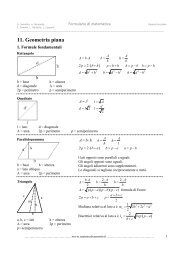
Le relazioni ottenute sono rappresentate graficamente in figura 3.1. 

Ogni stato di sforzo assegnato è rappresentato 

in tale figura da un punto di coordinate σ 1 e σ 2 , 

dove σ 1 e σ 2 sono i due sforzi principali. Se 

questo punto cade all’interno dell’area mostrata, 

il componente strutturale è sicuro. Se cade al di 

fuori di quest’area, il componente cederà per 

snervamento del materiale. L’esagono associato 

all’inizio dello snervamento nel materiale è noto 

come esagono di Tresca, la cui area è uguale a: 

2 

Λ = 3⋅ 

σ 

T Y 

Figura 3.1 

22


Criterio della massima energia di distorsione (criterio di Von Mises) 

Nel campo elastico, questo criterio si basa sulla determinazione dell’energia di distorsione 

di un dato materiale, cioè dell’energia associata alle variazioni di forma del materiale. 

Secondo questo criterio, noto anche come criterio di Von Mises (Richard Von Mises 1883- 

1953), un dato componente strutturale è sicuro fino a che il massimo valore dell’energia di 

distorsione per unità di volume in quel materiale rimane al di sotto dell’energia di 

distorsione per unità di volume che provoca lo snervamento in un provino del materiale 

sottoposto a trazione. 

Nel caso di un corpo generico soggetto allo sforzo delle sei componenti σ x , σ y , σ z , τ xy , τ xz e 

τ zy , la densità di energia volumica di deformazione può essere espressa come : 

1 

J 

u = ⋅( σ x ⋅ εx + σ y ⋅ εy + σz ⋅ εz + τxy ⋅ γ xy + τ xz ⋅ γ xz + τ zy ⋅ γ zy) 

dimensionalmente: 3 

2 

m 

ricordando dalla teoria dell’elasticità la legge costitutiva del materiale (figura 3.2): 

⎧ σ ν ⋅σ 

x y ν ⋅σz 

⎪ε 

x = − − 

⎪ 

E E E 

⎪ ν ⋅σ σ x y ν ⋅σ 

z 

⎪ε 

y =− + − 

⎪ 

E E E 

⎪ ν ⋅σ 

ν ⋅σ 

x y σ z 

⎪ε 

z =− − + 

⎪ E E E 

⎨ 

⎪ τ xy 

⎪ 

γ xy = 

G 

⎪ 

⎪ τ xz γ xz = 

⎪ G 

⎪ 

⎪ 

τ yz 

γ yz = 

⎪⎩ G 

modulo elastico trasversale: 

E 

G = 

2⋅ 1+ 

( ν ) 

Figura 3.2 

E Modulo elastico longitudinale (di Young) 

ν Coefficiente di contrazione trasversale (di Poisson) 

deformazione: scorrimento angolare: 

l−l0∆l ε = = 

l l 

d 

γ = = tanθ 

θ 

b 

0 0 

Il tensore di deformazione simmetrico si 

esprime: 

⎡ γ xy γ ⎤ xz 

⎢εx⎥ ⎢ 

2 2 

⎥ 

⎢γxy γ yz 

⎥ 

[ S ] = ⎢ ε y ⎥ 

⎢ 

2 2 

⎥ 

⎢γγ xz yz ⎥ 

⎢ ε z ⎥ 

⎢⎣ 2 2 ⎥⎦ 

Nel caso di trazione semplice: 

⎧ σ x ε 

⎪ x = 

E 

⎪ 

⎪ ν ⋅σ 

x 

⎨ε 

y =− 

⎪ E 

⎪ ν ⋅σ 

x 

⎪ε 

z =− 

⎩ E 

[3.2.1] 

con la conseguente dilatazione volumetrica: 

( 1−2⋅ν) ⋅σx 

ε = ε + ε + ε = 

x y z 

E 

23


Sostituendo i valori delle deformazioni ( ε x , ε y e ε z ) e degli scorrimenti angolari ( γ xy , γ xz e 

γ yz ) nella espressione [3.2.1]: 

2 2 2 1 2 2 2 

( σx σ y σz 2 ν ( σx σ y σ y σz σz σx) ) ( τxy τ yz τzx 

) 

1 

u = ⋅ + + − ⋅ ⋅ ⋅ + ⋅ + ⋅ + ⋅ + + 

2⋅ 

E G 

[3.2.2] 

Se come assi coordinati si utilizzano gli assi principali relativi al punto considerato, gli 

sforzi tangenziali si annullano, quindi: 

1 2 2 2 

u = ⋅ ( σ1 + σ2 + σ3 −2⋅ν ⋅( σ1⋅ σ2 + σ2⋅ σ3 + σ3⋅σ1) ) 

[3.2.3] 

2⋅ 

E 

La densità di energia u è uguale alla somma dell’energia associata alla variazione di 

volume nel punto considerato uv 

(dovuta agli sforzi normali di compressione), e all’energia 

associata alla distorsione u (dovuta agli sforzi di taglio) sempre nello stesso punto: 

= v + d 

d 

[3.2.4] 

uv d u 

u u u 

Al fine di calcolare 

considerato: 

e , si introduce il valor medio degli sforzi principali nel punto 

σ1 + σ2 + σ3 

σ = [3.2.5] 

3 

e si pone: 

' 

σ = σ + σ 

1 1 

σ = σ + σ 

' 

2 2 

[3.2.6] 

' 

σ 3 = σ + σ3 

Nel caso di soli sforzi di taglio, σ 1, 

σ 2 e σ 3 sono nulli. 

Dalla [3.2.5] e [3.2.6] si evince: 

' ' ' 

σ1 + σ2 + σ3 

= 0 

[3.2.7] 

ne consegue che la parte uv 

della densità di energia di deformazione che corrisponde ad 

una variazione di volume dell’elementino può essere ottenuta sostituendo σ a ognuno 

degli sforzi principali della [3.2.3]. 

uv 

( 3 σ 2 ν ( 3 σ ) ) 

2 

( ) 

1 

2 2 3⋅σ⋅ 1−2⋅ν = ⋅ ⋅ − ⋅ ⋅ ⋅ = 

2⋅E 2⋅E 

Sostituendo l’equazione [3.2.5] del valor medio: 

1−2⋅ν = ⋅( σ −σ −σ 

) 

uv 

6⋅ 

E 

1 2 3 

Quindi, l’energia di deformazione ud 

è espressa da: 

2 2 2 

2 

( 3 ( σ1 σ2 σ3 ) 6 ν ( σ1 σ2 σ2 σ3 σ3 σ1) ( 1 2 ν) ( σ1 σ2 σ3 

) 

1 

ud = u− uv 

= ⋅ ⋅ + + − ⋅ ⋅ ⋅ + ⋅ + ⋅ − − ⋅ ⋅ − − 

6⋅ 

E 

[3.2.8] 

[3.2.9] 

) [3.2.10] 

Elevando il quadrato della [3.2.10] e riordinando i termini: 

1+ 

ν 

= ⋅ 

2 2 

σ −2⋅σ ⋅ σ + σ + 

2 2 

σ −2⋅σ ⋅ σ + σ + 

2 

2 

σ −2⋅σ ⋅ σ + σ 

[3.2.11] 

ud 

6⋅ 

E 

( ( 1 1 2 2 ) ( 2 2 3 3 ) ( 3 3 1 1 ) ) 

Ciascuna delle espressioni in parentesi nella [3.2.11] rappresenta un quadrato perfetto ed 

essendo: 

E E 

G = ⇒ 1+ 

ν = 

2⋅ ( 1+ ν ) 2⋅G 

l’espressione [3.2.10] dell’energia di deformazione diventa: 

ud 

= 

1 

2 2 

2 

⋅( ( σ1 − σ2) + ( σ2 − σ3) + ( σ3 −σ1) 

) 

12⋅ 

G 

[3.2.12] 

Nel caso di sforzo piano, e supponendo che l’asse 3 (parallelo allo sforzo σ 3 ) sia 

perpendicolare al piano di sforzo, si ha σ 3 = 0 e l’equazione [3.2.12] si riduce a: 

ud 

1 

= ⋅ − + 

6⋅ 

G 

2 2 

( σ1 σ1σ2 σ2 

) 

[3.2.13] 

24


Considerando il caso particolare di un provino sottoposto a trazione, si nota che, allo 

σ = σ , σ 2 = 0 e quindi 

snervamento, si ha 1 Y 

2 

σY 

( ud 

) = [3.2.14] 

Y 

6⋅ 

G 

Il criterio della massima energia di distorsione per lo sforzo piano indica che uno stato di 

sforzo assegnato è sicuro fino a che ud < ( ud 

) , ovvero, sostituendo a u l’espressione 

Y 

d 

data dall’equazione [3.2.13], finchè: 

2 2 2 

σ1 − σσ 1 2 + σ2 < σY 

[3.2.15] 

Oppure, esplicitando la tensione di snervamento si ottiene: 

σ = σ − σ σ + σ 

Y 

2 2 

1 1 2 2 

La [3.2.15] rappresenta una conica, e per capire di quale conica si tratta, è necessario 

calcolare gli invarianti. 

Data una conica a centro di equazione: 

2 2 

a⋅ σ + b⋅ σ + c⋅σ ⋅ σ + d⋅ σ + e⋅ σ + f = 

1 2 1 1 2 0 

con abcde , , , , , f costanti. 

l’invariante lineare è dato dalla somma: 

I = a+ b = 2 

l 

per cui Il ≠ 0 . 

L’invariante quadratico è dato dal determinante: 

c 

1 

a 

1 − 

2 2 3 

Iq = ⇒ Iq 

= = 

c 

1 4 

b − 1 

2 2 

si deduce che I q > 0 . 

L’invariante cubico è dato dal determinante: 

c d 

1 

a 

1 − 0 

2 2 2 

c e 1 3 2 

Ic = b ⇒ Ic 

= − 1 0 = − σ Y 

2 2 2 4 

2 

d e 

0 0 −σ 

Y 

f 

2 2 

da cui si evince Ic ≠ 0 

I valori dei tre invarianti indicano che si tratta di una ellisse ruotata e con centro di 

simmetria nell’origine del sistema di riferimento. 

Quindi, la [3.2.15] indica i punti interni di una ellisse ruotata rispetto agli assi coordinati (fig. 

3.3) in cui la tensione di snervamento σ Y = 250 MPa ed è ruotata, rispetto agli assi 

cartesiani, di un angolo α : 

1 ⎛ c ⎞ 

α = arctan ⎜ ⎟ 

2 ⎝a−b⎠ Ne consegue che la [3.2.15] è ruotata di un angolo α : 

1 ⎛ −1 

⎞ 1 1 π π 

α = arctan ⇒ α = lim arctan ( x) 

⇒ α = ⋅ ⇒ α = 

⎜ ⎟ 

2 ⎝ 1 − 1 ⎠ 

2 x→∞ 

2 2 

Perciò l’ellisse, rappresentata in figura 3.3, è inclinata di 45° (indipendentemente dal 

valore dello snervamento σ Y ), e sulle bisettrici, dei quattro quadranti del piano cartesiano, 

di equazione σ 2 = σ1 

e σ 2 =− σ1 

giacciono gli assi principali dell’ellisse AB e CD , e i semiassi 

misurano: 

6 

OA = 2 ⋅ σY OC = ⋅ σY 

3 

4 

25


con il valore dei semiassi è possibile calcolare l’area dell’ellisse: 

2⋅π⋅ 3 

Λ = π ⋅OA⋅ OC = σ 

3 

2 

V Y 

l’eccentricità dell’ellisse è data, indipendentemente dalla tensione di snervamento σ Y : 

( 2 ) 

2 ⎛ 6 ⎞ 

⋅σ 2 2 

Y − ⎜ 

⋅σY 

⎟ 

OA OC 

3 ⎟ 

− ⎝ ⎠ 6 

ξ = ⇒ ξ = ⇒ ξ = 0,816 

OA 

2 ⋅σ 

3 

con la distanza focale ζ : 

⎛ 6 6 ⎞ 

F1 

⎜ 

⋅σY; ⋅σY 

⎟ 

3 3 ⎟ 

⎝ ⎠ 

⎛ 6 6 ⎞ 

F2 

⎜ 

− ⋅σY; − ⋅σY 

⎟ 

3 3 ⎟ 

⎝ ⎠ 

2⋅3 OF1 = OF2 = ξ ⋅ OA = σ Y 

3 

4⋅3 ζ = 2⋅ 

OF1 

= ⋅σY 

3 

Alla tensione di snervamento σ Y = 250 MPa si ottiene (fig. 3.3): 

σ − σ σ + σ < 250 ⇒σ − σ σ + σ < 62500 

2 2 2 2 2 

1 1 2 2 1 1 2 2 

OA = 2 ⋅250 

353,5 

6 

OC = ⋅250 

204,1 

3 

2⋅π⋅ Λ V = 

3 

3 2 

⋅250 

226724,9 

⎛250⋅ F1 ⎜ 

⎝ 3 

6 250⋅ ; 

3 

6 ⎞ 

⎟ 

F1 

⎠ 

204,12;204,12 

( ) 

⎛ 250⋅ 6 250⋅ 6 ⎞ 

F2 ⎜ 

− ; − ⎟ F2 

−204,12; −204,12 

3 3 ⎟ 

 

⎝ ⎠ 

500⋅ 3 

OF1 = OF2 

= 288,68 

3 

1000⋅ 3 

ζ = 2⋅ 

OF1 

= 577,35 

3 

Y 

( ) 

2 

Figura 3.3 

Nel caso di uno stato di sforzo generico, si deve utilizzare per u d l’espressione [3.2.12]. 

Il criterio della massima energia di distorsione è allora espresso dalla condizione: 

2 2 2 2 

( σ1 − σ2) + ( σ2 − σ3) + ( σ3 − σ1) < 2⋅ σY 

[3.2.16] 

indicante che uno stato di sforzo assegnato è sicuro se il punto di coordinate σ 1, 

σ 2 e σ 3 si 

trova all’interno della superficie definita dall’equazione: 

2 2 2 2 

( σ1 − σ2) + ( σ2 − σ3) + ( σ3 − σ1) = 2⋅ σY 

[3.2.17] 

Che può scriversi nella forma equivalente: 

2 2 2 2 

2⋅ σ1 + 2⋅ σ2 + 2⋅σ3 −2⋅σ1⋅σ2 −2⋅σ1⋅σ3 −2⋅σ2⋅σ3 −2⋅ σY= 

0 

[3.2.18] 

Oppure, si può esplicitare lo snervamento e scriversi: 

2 2 

2 

( σ1− σ2) + ( σ2 − σ3) + ( σ3 −σ1) 

σ = 

Y 

2 

26


La [3.2.18] rappresenta la superficie di una quadrica, e per individuare di quale tipo di 

quadrica si tratta, è indispensabile ricorre alla matrice associata e all’invariante. 

Data l’equazione generale di una quadrica: 

2 2 2 

a11 ⋅ σ1+ a22 ⋅ σ2+ a33 ⋅ σ3+ 2⋅a12 ⋅σ1⋅ σ2+ 2⋅a13 ⋅σ1⋅ σ3+ 2⋅a23 ⋅σ2⋅ σ3+ 2⋅a14 ⋅ σ1+ 2⋅a24 ⋅ σ2+ 2⋅a34 

⋅ σ3+ 

a44 

= 0 

il determinante della matrice simmetrica, associata all’equazione della quadrica, è 

rappresentato: 

a11 a12 a13 a 2 −1 −1 

0 

14 

a 1 2 1 0 

12 a22 a23 a − − 

24 

M = = = 0 

a a a a −1 −1 

2 0 

13 23 33 34 

a14 a 0 0 0 24 a34 a44 −2⋅σY 2 

Il valore di questo determinante è nullo, ciò implica che si tratta di una quadrica degenere; 

quindi, l’equazione[3.2.18] può essere un cilindro (ellittico, parabolico o iperbolico) o un 

cono quadratico. 

Ora si verifica se ha è una quadrica a centro, cioè dotata di un centro di simmetria: 

a a a 2 −1 −1 

11 12 13 

A = a a a = −1 

2 − 1 = 0 

12 22 23 

a a a 

13 23 33 

−1 −1 

2 

Essendo nullo, ciò implica che la quadrica non ha centro di simmetria, per cui si esclude la 

possibilità che sia un cono, quindi la [3.2.18] è l’equazione di un cilindro. 

Per determinare di quale tipo di cono si tratta è necessario stabilire il rango della matrice 

A ; poiché il determinante è nullo, il rango rA ≤ 2 . Se un minore, di dimensione 2, della 

matrice A è diverso da zero, il rango r A = 2 . 

a a 

11 12 

a a 

12 22 

2 −1 

= = 3≠ 0 

−1 

2 

il valore di questo determinante è diverso da zero, per cui il rango è 2; quindi il cilindro può 

essere ellittico (o a sezione circolare) o iperbolico. 

Se l’invariante quadratico è strettamente maggiore di zero, la [3.2.18] è un cilindro ellittico, 

altrimenti iperbolico: 

a a 2 −1 

I = ⇒ I = = 3⇒ I q > 0 

−1 

2 

11 12 

q 

a12 a22 

q 

la [3.2.18] rappresenta un cilindro ellittico. 

Per stabilire se le generatrici del cilindro ellittico sono inclinate rispetto al sistema di 

riferimento, è sufficiente adoperare almeno due sezioni, al cilindro, con un piano 

perpendicolare all’asse σ 3 e osservare come sono posizionati i centri delle ellissi, ottenute 

con le sezioni. 

Prima sezione: 

2 2 2 2 

⎧⎪ 2⋅ σ1 + 2⋅ σ2 + 2⋅σ3 −2⋅σ1⋅σ2 −2⋅σ1⋅σ3 −2⋅σ2⋅σ3 −2⋅ σY= 

0 

⎨ 

⎪⎩ σ 3 = 0 

si ottiene l’ellisse di equazione: 

2 2 2 

σ1 + σ2 −σ1⋅σ2 − σY= 

0 

analoga alla[3.2.15] e di centro 1 ( ) 0,0,0 C 

Seconda sezione: 

σ σ σ σ σ σ σ σ σ σ 

2 2 2 2 

⎧⎪ 2⋅ 1 + 2⋅ 2 + 2⋅ 3 −2⋅ 1⋅ 2 −2⋅ 1⋅ 3 −2⋅ 2⋅ 3 −2⋅ Y = 0 

⎨ 

⎪⎩ σ 3 = K 

con la costante K ∈ si ottiene il fascio di ellissi di equazione: 

2 2 2 2 

σ + σ −σ ⋅σ −K⋅σ −K⋅σ − σ + K = 

1 2 1 2 1 2 Y 0 

rappresentato in figura 3.4, in cui si sono disegnate venti ellissi per: 

K =−10; −9; −8; −7; −6; −5; −4; −3; −2; − 1;0;1;2;3;4;5;6;7;8;9;10 con σ = 250 MPa . 

Y 

27


Il centro C ( , , K) 

σ σ : 

2 10 20 

c 

2 

d 

2 

1 

− 

2 

K 

− 

2 

σ10 

= 

b 

a 

e 

2 

c 

2 

= 

1 

1 

K 

− 

2 

1 

− 

2 

= K 

c 

2 

b 

1 

− 

2 

1 

a 

d 

2 

1 

K 

− 

2 

c 

σ 

2 

20 =− 

a 

e 

2 

c 

2 

1 

− 

=− 

2 

1 

K 

− 

2 

1 

− 

2 

= K 

c 

2 

b 

1 

− 

2 

1 

Figura 3.4 

Quindi, questa seconda ellisse ha il centro C2 ( K, K, K ) ; ciò significa che i centri C1 e 2 è 

come se fossero disposti sulle due estremità della diagonale di un cubo, per cui, i centri 

delle infinite ellissi che si possono ottenere sezionando il cilindro con i piani 

C 

3 K σ = (fig. 

3.10), sono disposti lungo una retta passante per l’origine del sistema di riferimento e 

individuata dall’intersezione dei due piani: 

⎧σ2 

= σ1 

⎨ 

⎩σ 

3 = σ1+ σ2 

I coseni direttori lungo i tre assi di riferimento σ 1, 

σ 2 e σ 3 : 

⎧ K 

3 

⎪cosω1 

= ⇒ cosω1 

= 

⎪ ρ 

3⋅ 

K 

⎪ K 

3 

⎨cosω2 

= ⇒ cosω1 

= 

⎪ ρ 

3⋅ 

K 

⎪ 

K 

3 

⎪ cosω3 = ⇒ cosω1 

= 

⎪⎩ ρ 

3⋅ 

K 

ρ 

2 2 2 2 

= + + = ⋅ 

K K K K 

3 

Si conclude che le generatrici del cilindro sono inclinate di 45° rispetto al piano σ 3 = 0 , e 

quindi l’asse di simmetria forma angoli uguali ( di 45°) con i tre assi principali di sforzo σ 1, 

σ 2 e σ 3 . 

La sezione normale al cilindro è una circonferenza con il raggio coincidente con il 

semiasse minore OC dell’ellisse (ottenuta con la sezione del cilindro con il piano σ 3 = 0 ) 

che misura 6/3⋅ σ Y (fig. 3.5). 

L’equazione della circonferenza, della sezione circolare del cilindro, è data (fig. 3.6): 

⎛ 6 ⎞ 

2 

σ + σ = 

⎜ 

⋅σ ⇒ σ + σ = ⋅ 

3 ⎟ 

σ 

⎝ ⎠ 

3 

2 

2 2 2 2 

2 

1 2 ⎜ Y ⎟ 1 2 

Y 

28



La [3.2.17] rappresenta una superficie di un cilindro di sezione trasversale circolare (fig. 

3.7 e 3.8) con l’asse di simmetria w che forma angoli di 45° con gli assi principali σ 1, 

σ 2 e 

σ 3 (fig.3.7). 

La [3.2.16] indica i punti del volume interno al cilindro. 



29


Confronto tra il criterio di Tresca e di Von mises 

Il criterio del massimo 

sforzo tangenziale e il 

criterio della massima 

energia di distorsione sono 

confrontati in figura 3.11. 

Si nota che l’ellisse passa 

per i vertici dell’esagono. 

Quindi, per gli stati di sforzo 

rappresentati da questi sei 

punti, i due criteri forniscono 

lo stesso risultato. 

Il rapporto tra le due aree, 

quella dell’ellisse e del 

esagono, evidenzia come il 

criterio di Von Mises sia più 

“tollerante” del criterio di 

Tresca, in quanto Figura 3.11 

2⋅π⋅ 3 2 

⋅σ 

Λ Y 

3 2⋅π⋅ 3 

= = 1, 209 

Λ ⋅ 

9 

V 

2 

T 3 σ Y 

L’ellisse di Von Mises ricopre una superficie maggiore del 20% circa, rispetto all’esagono 

di Tresca; il criterio di Tresca, quindi, si mostra più “severo” nel determinare se un 

materiale è sicuro, e quindi se ricade o meno all’interno dell’area dell’esagono. 

30


PARTE IV: introduzione ai processi di lavorazione meccanica 

Determinazione dei carichi per la trafilatura e la fucinatura da considerazioni 

tensionali: introduzione 

Il significato della teoria dei processi di lavorazione meccanica dei metalli è di poter 

prevedere la deformazione di un metallo e la forza richiesta per produrre tale 

deformazione. 

In aggiunta, una conoscenza degli sforzi locali (prova a trazione) e della deformazione 

plastica aiutano a predire le cause del cedimento del prodotto finito. Questi fattori 

controllano il tipo processo di lavorazione designato e la dimensione e forma delle matrici. 

I carichi per i processi di lavorazione e l’energia consumata sono notevolmente influenzati 

dalla combinazione appropriata dei parametri di processo che includono: i livelli di 

passaggio (durante una lavorazione metallurgica), lubrificazione, temperatura, velocità e la 

sezione dello stampo della matrice. 

La maggioranza dei sistemi di lavorazione sono troppo complessi per una completa 

trattazione teorica, così con l’ausilio di regole empiriche, le formule analitiche sono 

efficacemente più utilizzate con la conoscenza dei dati sperimentali. Per gran parte dei 

processi metallurgici di laminazione, forgiatura, estrusione e trafilatura è possibile 

prevedere i carichi di lavoro con buona precisione. 

In questa relazione saranno discussi i due metodi di stima dei carichi da applicare nei 

processi di lavorazione, dall’analisi degli sforzi. 

Lavoro per variare la lunghezza di un elemento rettilineo 

Un generale approccio, applicabile alla semplice tensione o compressione, e anche a più 

complessi processi di lavorazione come il filo metallico della trafilatura, è valutato nel 

lavoro compiuto dalla deformazione plastica di un piccolo elemento del pezzo da lavorare, 

e quindi dall’integrare del tutto l’intera curva di deformazione. 

Per una tensione monoassiale σ Y (trazione o compressione) gli sforzi principali sono così 

determinati: 

⎧σ 

1 = σY 

⎪ 

⎨σ 

2 = 0 

⎪ 

⎩σ 

3 = 0 

Sotto questo sforzo assiale (in tensione o compressione) la lunghezza di un elemento 

monodimensionale, in cui una dimensione è predominante sulle altre due, è variata da L 

a L + dL ; il lavoro infinitesimo δ W è quindi esprimibile come: 

δ W = FdL 

[4.1.1] 

in cui F è il carico totale assiale agente sull’elemento. 

Poiché: 

F = σ Y ⋅ A 

indicando con A la sezione trasversale dell’elemento, l’espressione del lavoro diventa: 

δW = ( σY⋅A) 

dL [4.1.2] 

Inoltre, essendo: 

dL = Ldε 

sostituendola nella [4.1.2] l’espressione del lavoro è data dall’equazione: 

δW = ( σY⋅ A) Ldε 

[4.1.3] 

31


Dove il prodotto tra l’area e la lunghezza esprime il volume: 

V = A⋅ L 

Quindi, sostituita nella [4.1.3] l’espressione del lavoro diviene: 

δW = ( σY⋅ V) dε 

[4.1.4] 

Per una variazione finita della deformazione si ha: 

ε1 

∫ ( σ Y ) dε 

[4.1.5] 

W = ⋅V 

ε0 

E con il volume costante, si ottiene l’energia per unità di volume, cioè 

W 

V 

3 

⎡ ⎤ 

⎣J/ m⎦ 

: 

ε1 

= ∫ σ Y dε 

[4.1.6] 

ε0 

Da notarsi l’uso del differenziale non esatto δ , in quanto la quantità infinitesima di lavoro 

non è il differenziale di una funzione (ad esempio di coordinate termodinamiche PVT), 

bensì un differenziale non esatto; infatti nel campo plastico un provino sottoposto a 

trazione, una volta scaricato, non ritornerà alla configurazione iniziale (vi è una 

deformazione permanente), ed anche in campo elastico vi è sempre una piccolissima 

deformazione residua. 

Se il carico esterno viene applicato 

lentamente, la trasformazione è 

essenzialmente quasi statica; si può 

quindi utilizzare un’equazione di stato per 

esprimere σ Y in funzione di ε , così da 

poter eseguire l’integrazione. La figura 4.1 

mostra una tipica curva sforzo – 

deformazione per un metallo in tensione. Il 

lavoro per unità di volume dell’elemento 

considerato a volume costante deformato 

per la tensione da ε 0 a ε 1 è rappresentato 

dall’area sotto il tratto di curva compreso 

tra i punti σ 0 e σ 1. 

L’andamento rettilineo 

del diagramma rappresenta la legge di 

Hooke. Figura 4.1 

Considerando ε reale, quindi ε reale , cioè la deformazione riferita alla effettiva variazione 

della lunghezza e della sezione dell’elemento sottoposto allo sforzo σ Y , si ottiene: 

dL L 

ε reale = ε = = = + ε 

ε0 

L0 

L L 

ε1 

L1 

1 

∫ d ∫ ln ln ( 1 ) 

[4.1.7] 

0 

L’espressione [4.1.6] può scriversi come: 

W 

= 

L1 

dL 

σ ⋅ 

[4.1.8] 

∫ 

Y 

V L0 

L 

Sviluppando: 

W dL L 

= σ ⋅ = σ ⋅ = σ ⋅ + 

V L L 

L1 

1 

∫ ln ln ( 1 ε ) 

[4.1.9] 

Y 

L 

Y Y 

0 

0 

Quest’ultima equazione, spesso nota come l’espressione del lavoro, fornisce una 

ragionevole approssimazione per un metallo il quale è stato lavorato duramente prima 

dell’allungamento a trazione, così che σ y (tensione di snervamento) non varia 

eccessivamente nel processo. Ciò è meno attendibile per un materiale ricotto, in cui il 

rapido incremento con la tensione (per cui è preferibile usare l’espressione [4.1.6] o 

[4.1.8]) integra la curva sforzo – deformazione graficamente o numericamente (infatti il 

32


tratto dopo lo snervamento è praticamente orizzontale). Questo metodo può essere 

applicato ad alcune operazioni pratiche. 

Dopo la strizione, non essendoci variazione di volume durante la deformazione plastica: 

A0⋅ L0 = A1⋅ L1 

si ha, sostituendolo nella [4.1.7]: 

ε 

⎛ A ⎞ 

0 

reale = ln ⎜ ⎟ 

A1 

⎝ ⎠ 

Dalla [4.1.9] esplicitando W si ottiene: 

L 

[4.1.10] 

1 

= ⋅σY⋅ ln 

[4.1.11] 

L0 

W V 

E osservando che il lavoro svolto dalla forza del processo di trafilatura in movimento dalla 

posizione iniziale, adiacente alla matrice, alla lunghezza completa L1 

del filo d’uscita, è 

dato da: 

W1 = F⋅ L1 

[4.1.12] 

Esplicitando dalla [4.1.12] la forza F sostituendo al lavoro W1 

l’espressione [4.1.11]: 

F 

V 

L 

1 

= ⋅σY⋅ ln 

[4.1.13] 

L1 L0 

Come già detto prima, nel campo plastico non vi è variazione di volume, quindi: 

V A L A L 

= 0⋅ 0 = 1⋅ 1 

[4.1.14] 

Il quale sostituito nella [4.1.13]: 

L 

1 

= 1 ⋅σY⋅ ln 

[4.1.15] 

L0 

F A 

Dalla [4.1.7] e [4.1.10] la deformazione reale ε reale è: 

ε 

L 

⎛ A ⎞ 

1 

0 

reale = ln = ln ⎜ ⎟ 

L0 A1 

⎝ ⎠ 

Quindi la [4.1.15] può esprimersi come: 

⎛ A ⎞ 

0 

= 1 ⋅ Y ⋅ln ⎜ ⎟ 

A1 

F A 

σ 

⎝ ⎠ 

Ora, introducendo il fattore di riduzione r dell’area della sezione: 

r 

A − A A 

[4.1.16] 

[4.1.17] 

0 1 1 

= = 1− 

[4.1.18] 

A A 

0 0 

L’espressione della forza [4.1.17] diventa: 

⎛ 1 ⎞ 

F = A1⋅σY⋅ln 

⎜ ⎟ 

[4.1.19] 

⎝1−r⎠ Lo sforzo principale σ 1 è conseguentemente: 

F ⎛ 1 ⎞ 

σ1= = σY⋅ln 

⎜ ⎟ 

[4.1.20] 

A ⎝1−r⎠ 1 

Questo risultato costituisce la base del calcolo nel processo della trafilatura, correzioni da 

applicare per prendere ragione dell’influenze dei vincoli meccanici e delle frizioni della 

macchina di lavorazione. 

33


Applicazione dell’equazione del lavoro: determinazione della massima possibile 

riduzione di una sezione in un unico passaggio 

La trafilatura di un filo metallico è limitata eventualmente dal cedimento (microfessurazioni) 

in trazione del filo trafilato. Durante un passaggio nella lavorazione metallurgica, così 

gravosa, il massimo sforzo di trazione sarà più vicino all’uguagliare la sua tensione di 

snervamento, a causa dell’incrudimento che il filo trafilato ha subito. Così, al limite di 

riduzione: 

σ = σ 

1 Y 

l’andamento dell’incrudimento sarà piccolo, così che lo sforzo medio di snervamento σ Y 

sarà anche vicino all’uguagliareσ Y . La massima riduzione rm 

è così data dalle condizioni: 

σ1 

= 1 

σ 

Y 

1 

σ1= σY ⋅ ln 

1−r 1 

= σY 

ln 

1−r 

affinchéσ 1 = σ Y : 

1 

ln 

1−rm così: 

1 

= 1 ⇒ 

1−rm 

= e 

1 

1− 

r 

= e 2,7182818284.... 

r 

m 

m 

m m 

1 

= 1− 0,6321205588.... 

e 

La massima riduzione possibile, con una perfetta lubrificazione, è del 63% o leggermente 

maggiore se l’andamento dell’incrudimento è ancora considerevole. 

34


Estrusione di una sbarra 

L’equazione del lavoro [4.1.11] può anche essere usata per ottenere il più basso limite alla 

pressione di estrusione, assumendo la deformazione omogenea e l’attrito nullo. 

Nell’estrusione, la forza è applicata alla billetta iniziale, di area A0 

, non al prodotto di cui 

l’area è A1 

come era nella trafilature dell’esempio di sopra. Questa forza spinge attraverso 

una distanza L0 

pari alla lunghezza della billetta e così il lavoro è: 

W0 = ( p⋅A0) ⋅ L0 

il quale è uguagliato al lavoro della deformazione omogenea: 

L 

W = V ⋅σ ⋅ = V ⋅σ ⋅ 

in cui: 

A0 

p = σY 

⋅ ln 

A 

A 

1 

0 

Y ln Y ln 

L0 A1 

1 

Si vedrà in seguito che il limite più basso è una insufficiente approssimazione per 

l’estrusione perché il fattore di costrizione è alto per tutte le utili estrusioni di rapporto 

A0 / A 1. 

E’ possibile calcolare la massima riduzione dell’area, come per la trafilatura, basata sul 

limite p = σ Y , che implica una compressione nella superficie della matrice. 

Ciò è importante nella estrusione a stampo aperto, usata per giunti imbullonati e altri 

elementi di fissaggio, ma nella maggior parte delle estrusioni p = σ Y non è più sufficiente a 

garantire l’estrusione. 

35


PARTE V: il processo di trafilatura 

Processo di trafilatura: introduzione 

Il processo di trafilatura (vedi figura 5) è attuato mediante un motore elettrico, che 

fornendo una coppia al blocco-motore, avvolge il filo trafilato, il quale passa attraverso uno 

stampo (o matrice) riducendosi di sezione a causa della forza di trazione provocata dalla 

rotazione del blocco-motore; il filo da trafilare è avvolto su un tamburo in cui non è 

applicata alcuna coppia motore, e durante il processo di trafilatura si srotola sotto l’effetto 

dell’avvolgimento del secondo tamburo collegato al motore. 

Il processo di trafilatura si realizza di norma a temperatura ambiente (circa 20° C) e più 

raramente a alta temperatura. Qui sarà trattato il caso di lavorazione a temperatura 

ambiente. 

E’ bene precisare che la velocità di uscita del filo trafilato dalla matrice è costante, e 

normalmente assume i valori compresi tra 1 e 10 m/s (a seconda del valore di B e della 

temperatura a cui si sta lavorando), per cui: 

dv 

v = Kost ⇒ a = = 0⇒ ∑ F = 0 

dt 

quindi il sistema è in equilibrio. 

Figura 5 

36


Sbarra cilindrica trafilata con una matrice conica 

La figura 5.1 mostra gli sforzi agenti su un sottile tronco (a simmetria cilindrica), ad una 

distanza x dalla apertura della matrice conica (con α, µ, σ y costanti). 

Figura 5.1 

Da prime considerazioni geometriche si ha: 

D ⋅cotα 

⎧ a 

⎪xa 

= 

2 

⎪ 

⎪ Db 

⋅cotα 

⎨xb 

= 

⎪ 2 

⎪ ( Db −Da) ⋅cotα 

⎪xb 

− xa 

= 

⎩ 

2 

Ci sono tre componenti di sforzo 

agenti nella direzione assiale: 

1) dovute al cambiamento dello 

sforzo longitudinale 

2) dovute direttamente alla pressione 

della matrice sulla circonferenza 

della sezione della sbarra 

3) dovute all’attrito della trazione alla 

circonferenza 

Per quanto riguarda il primo punto, lo sforzo agente lungo la direzione assiale, è 

esprimibile mediante la relazione (da notare che Da < D< Db): 

2 2 

⎛ D+ dD⎞ ⎛ D⎞ 

π 

( σx + dσx) ⋅ ⋅π −σx ⋅ ⋅π ⇒ ( σ x + dσx) ⋅ ⋅ ( D+ 

2 π 

) − ⋅σx ⋅ 

2 

⎜ ⎟ ⎜ ⎟ 

dD D [5.1.1] 

⎝ 2 ⎠ ⎝ 2 ⎠ 

4 4 

Il secondo punto è espresso dalla relazione: 

p⋅ ⎛π⎞ ⎛ dx ⎛ D ⎞ 

⎜ −α⎟⋅⎜ ⋅⎜ ⎟⋅ 2 cosα 2 

⎞ ⎛ dx ⎞ 

⋅π ⎟⇒ 

p⋅⎜π 

⋅D⋅ ⎟⋅ 

cosα 

cos 2 sin 

⎝ ⎠ ⎝ ⎝ ⎠ ⎠ ⎝ ⎠ 

α [5.1.2] 

in cui la grandezza dx /cosα 

è il segmento HK . 

Ed ancora, il terzo punto (riferito all’attrito µ ): 

⎛π⎞ ⎛ dx ⎛ D ⎞ ⎞ ⎛ dx ⎞ 

µ ⋅ p⋅ sin ⎜ + α⎟⋅⎜ ⋅⎜ ⎟⋅2⋅π ⎟⇒ 

µ ⋅ p⋅⎜π 

⋅D⋅ ⎟⋅cosα 

⎝ 2 ⎠ ⎝cosα ⎝ 2 ⎠ ⎠ ⎝ cosα 

⎠ 

Le condizioni, sotto trafilatura costante, devono essere in equilibrio. 

[5.1.3] 

Così, a meno del prodotto degli infinitesimi (si trascura l’infinitesimo dD elevato al 

quadrato), si ottiene, sommando la [5.1.1], [5.1.2] e la [5.1.3] l’equazione di equilibrio dello 

sforzo assiale: 

σx ⋅D⋅dD 2 

D ⋅dσx 

p D tanα dx µ p D dx 0 

2 

+ 

4 

+ ⋅ ⋅ ⋅ + ⋅ ⋅ ⋅ = [5.1.4] 

Poiché dD = 2⋅dx⋅ tanα, 

la [5.1.4] può riscriversi come: 

2⋅σx ⋅ dD + D ⋅ dσ x + 2⋅ p ⋅ dD + 2⋅µ 

⋅ p ⋅dD ⋅ cotα= 0 

[5.1.5] 

E raggruppandone i termini: 

σ x 2 ( σ x ( 1 µ cotα) 

) 

Dall’equilibrio radiale: 

D⋅ d + ⋅ + p⋅ + ⋅ ⋅ dD =0 [5.1.6] 

σ ⋅ π ⋅D⋅dx r 

( ) 

⎛ π ⋅D⋅dx ⎞ 

=−p⋅⎜ ⎟⋅cosα 

⎝ cosα ⎠ 

⎛ π ⋅D⋅dx ⎞ 

µ p ⎜ ⎟⋅sinα 

⇒ σ r = −p⋅ 1−µ ⋅tanα 

⎝ cosα 

⎠ 

+ ⋅ ⋅ ( ) 

[5.1.7] 

37


Dato il valore molto piccolo di µ ⋅ tanα 

è possibile trascurare tale termine; i valori 

comunemente assunti da µ e α sono: 

0,05 

tan 0,005 

6 o 

⎧µ 

 

⎨ ⇒ µ ⋅ α 

α 

⎩ 

Relazioni di grandezza per le misure di fig. 17: 

⎧0< 

B ≤0,5 

con B = µ ⋅ cotα 

e in virtù del valore che può assumere l’angolo α 

⎪ 

⎨0 

σY ≤ σx 

(normalmente 5°< α D > Da 

> 0 e 1,5 si stima l’intervallo in cui B può assumere tutti i possibili valori. Di 

norma B non supera quasi mai il valore di 0,5 ; per cui si può 

affermare 0

Inoltre lo stato degli sforzi è cilindrico, e gli assi principali sono: σ1 = σ x e σ 2 = σ3 = σ r = − p . 

E’ opportuno ricordare che quando due sforzi principali sono uguali, il sistema (delle 

tensioni) è equivalente a uno sforzo monoassiale combinato con uno sforzo idrostatico 

(uguale per tutti i punti dell’elemento considerato), così che lo snervamento si verifica al 

valore di σ Y . 

Tutti i criteri di snervamento devono fornire questo risultato: 

Von Mises: ( ) ( ) ( ) 

Tresca: ( ) 

2 2 2 2 

1 − 2 + 2 − 3 + 3 − 1 = 2⋅ Y 

σ σ σ σ σ σ σ 

1 1 

max 1 3 

2 2 Y 

τ = ⋅ σ − σ = Kost = σ 

E poiché σ 2 = σ 3 i due criteri coincidono. 

Conseguentemente nella sbarra trafilata σ1 − σ3 = σY, 

così: 

σ x + p = σY ⇒ p = σY 

−σ x 

Combinando questa condizione di snervamento [5.1.8] con la [5.1.6] si ottiene: 

[5.1.8] 

D⋅ dσx + 2⋅ ( σY 

+ P⋅B) ⋅ dD = 0 

[5.1.9] 

La quale rappresenta una equazione differenziale a variabili separabili, che sviluppata: 

B σx dσ x 

σY 

( 1 

dD 

= 2⋅ 

B) 

L’impostazione della soluzione di tale equazione è: 

⋅ − ⋅ + D [5.1.10] 

1 1 

d x 2 d 

B x Y ( 1 B) σ 

∫ = ⋅ 

⋅σ −σ ⋅ + ∫ D 

D 

Risolti i due integrali, la soluzione generale di questa equazione differenziale è: 

[5.1.11] 

1 

⋅ln ( B⋅σx −σY ⋅ ( 1+ B) ) = 2⋅ ln ( D) 

+Kost [5.1.12] 

B 

Determinazione della costante ( Kost ) imponendo la trafilatura senza variazione di sezione 

all’interno della matrice dello stampo: 

2⋅B 

σ Y ⋅ ( 1+ 

B) 

D D σ 0 σ ( 1 B) D Kost Kost 

= ⇒ = ⇒ − ⋅ + = ⋅ ⇒ = − [5.1.13] 

b x Y b 2⋅B 

Db 

Sostituendo il valore della costante nell’equazione [5.1.12]: 

1 

ln ( B σ σ ( 1 B) ) 2 ln ( D) 

σ Y ⋅ ( 1+ 

B) 

2⋅ 

⋅ ⋅ − ⋅ + = ⋅ − [5.1.14] 

B D 

x Y B 

b 

Esplicitando lo sforzo σ x (normale alla sezione trasversale del trefolo): 

2⋅B 

⎛ ⎞ 

1+ 

B ⎛ D ⎞ 

σx = σY 

⋅ ⋅⎜1−⎜ ⎟ ⎟ 

B ⎜ D ⎟ 

⎝ ⎝ b ⎠ ⎠ 

[5.1.15] 

38


Quindi lo sforzo σ x varia al variare del diametro all’interno della matrice della trafilatura; 

spostandosi dall’ingresso verso la fine della matrice, σ x cresce al decrescere di D , 

ovvero, all’aumentare della riduzione del diametro della matrice. 

Lo sforzo σ x è uguale alla tensione i snervamento σ Y quando il generico diametro D , 

della sezione circolare della matrice conica (fig. 5.1), assume il valore: 

2⋅B 

⎛ ⎞ 

1 

1+ 

B ⎛ D ⎞ 

− 

σ 1 1 ( 1) 2 B 

x = σY 

⇒ ⋅⎜ − ⎟ D Db B ⋅ 

⎜ ⎟ = ⇒ = ⋅ + 

B ⎜ D ⎟ 

⎝ ⎝ b ⎠ ⎠ 

[5.1.16] 

Si noti come nel caso limite, in cui la generica sezione di diametro D coincide con la 

sezione di ingresso della matrice di diametro D , si ottiene lo sforzo applicato nullo: 

2⋅B 

⎛ ⎞ 

1 B ⎛ ⎛ D ⎞ ⎞ 

lim ⎜ 

+ 

σ Y ⋅ ⋅⎜1− ⎜ ⎟ ⎟⎟= 

0 

→ b ⎜ B ⎜ ⎝D ⎟ b ⎠ ⎟ 

⎝ ⎝ ⎠⎠ 

D D 

b 

39


Figura 5.2 

Figura 5.3 

In figura 5.2 e 5.3 sono riportate due micrografie di un acciaio che ha subito un processo 

di trafilatura; da notarsi i grani molto allungati e orientati verso la direzione dello sforzo di 

trazione applicato dalla motore elettrico. In entrambi i casi si è usato un attacco Nital, e 

nella prima micrografia (fig. 5.2) l’ingrandimento è di 200X mentre nella seconda (fig. 5.3) 

è di 400X. 

40


In termini di riduzione di area ( r ): 

π 

( Db Da 

) 

⋅ − 

4 

⎛D⎞ a 

r = ⇒ r = 1−⎜ 

π 

⎟ 

2 

⋅ D 

⎝ Db 

⎠ 

b 

4 

2 2 2 

La [5.1.15] diventa: 

σ xa 1+ 

B 

B 

( 1 ( 1 r) 

) 

σ Y B 

Esplicitandola riduzione di area r : 

[5.1.17] 

= ⋅ − − [5.1.18] 

( B 1) 

B 

σ ⋅ ( B + 1) 

⎛σY ⋅ + − ⋅σ 

⎞ x 

r = 1−⎜⎜ 

⎟ 

⎝ Y 

⎠ 

1 

B 

a [5.1.19] 

Anche in questo caso, per la [5.1.18], se nel caso limite di Db Da 

= e quindi le sezioni di 

ingresso e di uscita sono uguali, si avrà lo sforzo applicato σ xa nullo: 

⎛ 1+ 

B 

B ⎞ 

lim⎜σY⋅ ⋅( 1−( 1− r) 

) ⎟= 

0 

r→0 

⎝ B 

⎠ 

Lo sforzo σ xa è uguale alla tensione i snervamento σ Y quando la riduzione di area 

assume il valore: 

( ( ) ) ( ) 1 

σxa σY 

1+ 

B 

1 1 

B 

r 1 r 1 B 

− 

1 B 

= ⇒ ⋅ − − = ⇒ = − + [5.1.20] 

B 

Sostituendo la [5.1.17] nella [5.1.20] si ricava l’uguaglianza σ xa = σ Y in funzione dei diametri 

di ingresso e di uscita, dalla matrice, del filo trafilato: 

⎧ 

1 1 

− − 

( ) ( ) 2 

2 

D 1 B 1 B 

a Db B Da Db B ⋅ 

⎪ = ⋅ + ⇒ = ⋅ + 

⎛ 1 

D ⎞ a 

− ⎪ 

1− 1 ( B 1) 

B 

1 

⎜ ⎟ = − + ⇒⎨ Da 

[5.1.21] 

D 

( 1) 

2 B 

b 

Db Db Da B ⋅ 

⎝ ⎠ ⎪ = ⇒ = ⋅ + 

1 

− 

⎪ ( B + 1) 

B 

⎩ 

In funzione dello snervamento σ Y e del generico diametro D , si può calcolare, per la 

[5.1.15], in quale direzione la funzione σx = f ( σY, 

D) 

aumenta più rapidamente in un 

generico punto P( σ , D ) . 

Y 0 0 

Calcolo del gradiente ∇ f ( σ , D) 

della funzione σ σ 

Y 

2⋅B 

⎛ ⎞ 

1+ 

B ⎛ D ⎞ 

= ⋅ ⋅⎜1−⎜ ⎟ ⎟ 

B ⎜ D ⎟ 

⎝ ⎝ b ⎠ ⎠ 

x Y 

( σ , ) ( σ , ) ( 1) ⎛ D ⎞ 2 σ ( 1) 

2⋅B2⋅B ∂f Y D ∂ f Y D B+ ⎛ ⎞ ⋅ Y ⋅ B+ 

⎛ D ⎞ 

∇ f ( σ Y , D) 

= i+ j= ⋅⎜1−⎜ ⎟ ⎟i− 

⋅⎜ 

⎟ 

∂σY ∂D B ⎜ ⎝ D ⎟ b ⎠ D ⎝ D 

⎝ ⎠ 

b ⎠ 

Per il generico punto P( σ , D ) il gradiente è equivalente a: 

Y 0 0 

( B+ 1) ⎛ ⎞ 2⋅σ⋅ ( B+ 

1) 

2⋅B 2⋅B 

: 

j [5.1.22] 

⎛D ⎞ 0 Y 0 ⎛D ⎞ 0 

∇ f ( σ Y 0, D0) 

= ⋅⎜1−⎜ ⎟ ⎟i− 

⋅⎜ 

⎟ j [5.1.23] 

B ⎜ ⎝D ⎟ b ⎠ D0⎝D ⎝ ⎠ 

b ⎠ 

Ora si può calcolare la rapidità di variazione di σ = f ( σ , D) 

nel generico punto P( σ , D ) : 

x Y 

2 

2⋅B 2⋅B 

2 

∇f ( σY 

0, D0) 

⇒ 

⎛( B+ 1) ⎛ ⎛D ⎞ 

⎜ 0 

⋅⎜1− ⎜ ⎟ 

⎜ B ⎜ D 

⎝ ⎝ 

⎞⎞ ⎟⎟ ⎟⎟ ⎠⎠ ⎛ 2⋅σY0⋅ ( B+ 

1) 

⎛D ⎞ 0 

+ ⎜− 

⋅⎜ 

⎟ 

⎜ D D 

⎝ 

che si verifica nella direzione (derivata direzionale): 

⎛ ⎞ 

⎝ b ⎠ 0 ⎝ b ⎠ 

⎞ 

⎟ 

⎟⎠ 

Y 0 0 

r 

[5.1.24] 

2⋅B2⋅B 1 ⎛D ⎞ 0 2⋅σ 

⎛ Y 0 D ⎞ 0 

Df( ) ⎜1⎟ u σ Y0,D0 = ⋅ −⎜ ⎟ i− ⋅⎜ 

⎟ j [5.1.25] 

B ⎜ D ⎟ b D0Db ⎝ ⎝ ⎠ ⎠ ⎝ ⎠ 

41


Legami sforzo – deformazione nel processo di trafilatura 

Poiché il volume del filo trafilato varia pochissimo dopo lavorazione (in quanto dopo lo 

snervamento le variazioni di volume sono trascurabili), si può imporre: 

V = V 

i u 

cioè, il volume di ingresso e di uscita dalla matrice è lo stesso, per cui: 

⎛Db⎞ Vi= ⎜ ⋅πl 

2 

⎟ ⋅ 

⎝ ⎠ 

V 

⎛Da⎞ = ⎜ 

2 

⎟ 

⎝ ⎠ 

⋅π⋅l 


u x 

2 

2 

2 2 

b a 

⎛D ⎞ ⎛ D ⎞ 

⎜ ⋅π⋅ l = ⋅π⋅l 2 

⎟ ⎜ 

2 

⎟ 

⎝ ⎠ ⎝ ⎠ 

la lunghezza incognita l x è: 

x 

2 

Db⋅l lx 

= 2 

Da 

Per il calcolo della deformazione ε si suppone l = 1 mm : 

2 

Db 

−1 

2 2 2 

lx−l Da Db −Da 

ε = ⇒ ε = ⇒ ε = 2 

l 1 

Da 

per una generica sezione di diametro D interna alla matrice (stampo): 

2 2 

Db−D ε = [5.2.1] 

2 

D 

esplicitando il diametro D : 

D = 

Db 

⋅ ε + 1 

ε + 1 

sostituita alla [5.1.15]: 

2⋅ 

1+ B ⎛ ε + 1⎞ 

σx = σY 

⋅ ⋅ 1−⎜ 

B ⎜ ⎟ 

ε + 1 ⎟ 

B 

⎛ ⎞ 

⎜ ⎟ 

⎜ ⎝ ⎠ ⎟ 

⎝ ⎠ 

oppure può esprimersi: 

1 

( 1 ( 1) ) 

B 

σx σY + B 

ε 

− 

[5.2.2] 

= ⋅ ⋅ − + [5.2.3] 

B 

Esprimendo la deformazione ε in funzione della tensione di snervamento σ Y e dello sforzo 

σ applicato dal processo di trafilatura: 

x 

( 1 B) B 

ε 

σ Y ⋅ ( 1+ 

B) 

Ricordando che: 

1 

− 

B 

⎛σY ⋅ + − ⋅σ 

⎞ x 

= ⎜ ⎟ −1 

⎜ ⎟ 

⎝ ⎠ 

cosα 

B = µ ⋅ cotα 

= µ ⋅ 

sinα 

[5.2.4] 

Analizzando i casi limite del coefficiente B in funzione dell’angolo α (fig. 5.1) e con l’attrito 

µ costante, per un angolo infinitamente piccolo si ottiene: 

cosα 

lim µ ⋅ = +∞ 

sinα 

+ 

α →0 

per un angolo α massimo possibile, di 90°, si ottiene: 

cosα 

lim µ ⋅ = 0 

α→π /2 sinα 

42


Applicando questi due casi limite alla deformazione ε , si avrà: 

( 1 B) B 

σ ⋅ ( 1+ 

B) 

1 

− 

B 

⎛σY ⋅ + − ⋅σ 

⎞ x 

lim ⎜ − 1 = 0 

B→+∞⎜ 

⎟ 

⎝ Y 

⎠ 

cioè: 

ε = 0 nel caso di un angolo α infinitamente piccolo; in pratica il diametro del filo di 

min 

ingresso è uguale al diametro del filo di uscita (trafilato). 

Invece per un angolo α massimo, e cioè di 90°, si ottiene: 

( 1 B) B 

σ ⋅ ( 1+ 

B) 

1 

− 

B 

x 

⎛σY ⋅ + − ⋅σ 

⎞ x 

σY 

lim ⎜ − 1 = e −1 

B→0 

⎜ ⎟ 

⎝ Y 

⎠ 

σ 

quindi, la deformazione massima in funzione dello sforzo applicato e della tensione di 

snervamento si esprime: 

σY 

ε = e − 1 

max 

σ 

xa 

con e indicante il numero di nepero (2,71828182845....). 

Quindi, la deformazione (nel processo di trafilatura) risulta sempre compresa tra i valori: 

σ 

xa 

σY 

0< ε e −1 

[5.2.5] 

Supponendo che lo sforzo σ xa applicato dal processo di trafilatura sia uguale alla tensione 

di snervamento σ Y del filo, si avrà: 

1 

− 

⎛σ ( 1 

B 

1 

Y ⋅ + B) −B⋅σ ⎞ xa 

lim ⎜ − 1 = ( B + 1) B −1 

σxa →σ 

⎜ ⎟ 

Y σ Y ⋅ ( 1+ 

B) 

⎟ 

⎝ ⎠ 

per cui la deformazione nel caso di uguaglianza tra lo sforzo applicato e la tensione di 

snervamento si esprime: 

( ) 1 

ε = B + 1 B − 1 

[5.2.6] 

Applicando un esempio numerico, con i seguenti valori dei coefficienti: 

µ = 0,05 

⎧ 

⎪ o 

⎪α 

= 6 

⎪ ⎪B 

= µ ⋅ cotα = 0, 476 

⎨ 

⎪σ 

Y = 250 MPa 

⎪ σ xa = 325 MPa 

⎪ 

⎪⎩ σ R = 400 MPa 

si ottiene la deformazione dalla [5.2.4]: 

ε 2,13 mm/mm 

e la deformazione massima teorica dalla [5.2.5]: 

ε 2,67 mm/mm 

max 

43


Analizzando geometricamente la [5.2.3] si ottiene l’equazione in due variabili: 

−0,476 

σxa = σY⋅3,1008⋅ 1− ( ε + 1) 

[5.2.7] 

( ) 

con il grafico che segue: 



44


Con la tensione di snervamento costante, ad esempio di 250 MPa, la [5.2.7] diventa: 

−0,476 

σ = 775,2 ⋅ 1− ( ε + 1) 

xa 

( ) 

il cui grafico è rappresentato: 

SFORZO APPLICATO [MPa] 

400 

350 

300 

250 

200 

150 

100 

50 

0 

LEGAME SFORZO - DEFORMAZIONE 

NELLA TRAFILATURA 

0,0 0,5 1,0 1,5 2,0 2,5 3,0 3,5 

DEFORMAZIONE [mm/mm] 

Figura 5.8 

N.B.: sino a 1,3 mm/mm il comportamento di questo acciaio è elastico, successivamente, 

superando con lo sforzo applicato il limite di snervamento di 250 MPa (andando oltre la 

deformazione di 1,3 mm/mm) il comportamento è plastico e a 400 MPa vi è la rottura. 

45


Determinazione della massima riduzione di un trefolo 

Riduzione della sezione di ingresso nel caso di un generico sforzo applicato: 

⎧σ 

xa 1+ 

B 

B 

⎪ = ⋅( 1−( 1−r) 

) 

σY 

B 

⎪ 

⎨ 

1 

( 1 

B 

⎪ ⎛σY ⋅ B+ ) −B⋅σ ⎞ xa 

⎪r = 1−⎜⎜ 

⎟ 

σ Y ⋅ ( B + 1) 

⎟ 

⎩ ⎝ ⎠ 


( B 1) 

B 

σ ⋅ ( B + 1) 

1 

B 

⎛ ⎛σY ⋅ + − ⋅σ 

⎞⎞ 

xa 

r% 

= ⎜1− ⎟ ⋅100 

⎜ 

⎜ ⎟ ⎟⎟ 

⎝ ⎝ Y 

⎠⎠ 

Riduzione della sezione di ingresso nel caso di sforzo applicato calcolato come media 

aritmetica tra la tensione di snervamento e la tensione di rottura: 

⎧ σR + σY 

⎪σ 

xa = 

2 

⎪ 

⎨σR 

+ σY 

1 

2 1 1 

( 2) 

B 

⎪ + B B σR + σY 

+ B 

B ⎛σY ⋅ B+ −B⋅σR) ⎞ 

⎪ = ⋅( 1−( 1−r) ) ⇒ = ⋅( 1−( 1−r) ) ⇒ r = 1−⎜ 

⎟ 

σY B 2⋅σY B 

⎜ 2⋅σ 

( 1) 

⎟ 

⎪⎩ ⎝ Y ⎠ B ⋅ + 


1 

⎛ ⎞ 

( 2) 

B 

⎜ ⎛σY ⋅ B+ −B⋅σR) ⎞ ⎟ 

r% 

= 

⎜ 

1−⎜ ⋅100 

⎜ ⎟ 

2⋅σY⋅ ( B + 1) 

⎟ ⎟ 

⎜ ⎝ ⎠ ⎟ 

⎝ ⎠ 

Riduzione della sezione di ingresso nel caso che lo sforzo applicato coincida con la 

tensione di snervamento: 

( ( ) ) ( ) 1 

⎧σxa 

= σY 

⎪ 

⎨ 1+ 

B 

B 

− 

1 1 r 1 r 1 B 1 B 

⎪ ⋅ − − = ⇒ = − + 

⎩ B 


( ) 1 

⎛ − ⎞ 

r% = 1 B 1 B 

⎜ − + ⎟⋅100 

⎝ ⎠ 

46


Esempio di trafilatura 

Acciaio strutturale ASTM-A36 

Densità ρ 7860 

N 

Sforzo di rottura σ R 400 MPa = 4079 

2 

mm 

N 

Snervamento a trazione σ Y 250 MPa = 2549 

2 

mm 

N 

Snervamento a taglio σ YG 145 MPa = 1479 

2 

mm 

Modulo di elasticità normale E 200 

Modulo di elasticità tangenziale G 77 

Coefficiente di espansione termica χ 11,7 

Duttilità, percentuale di elongazione in 50 mm δ 23% 

Utilizzando parte dei dati dell’esempio precedente: 

µ = 0,05 

⎧ 

⎪ o 

⎪α 

= 6 

⎨ 

⎪B 

= µ ⋅ cotα = 0, 476 

⎪ 

⎩ Db 

= 3 mm 

Kg 

3 

m 

GPa 

GPa 

10 

° C 

−6 

N 

mm 

Kg 

2 

cm 

Kg 

2 

cm 

Kg 

2 

cm 

Kg 

cm 

3 

6 

= 10 ⋅ 2 2,03 ⋅ 10 

2 

N 

mm 

Kg 

cm 

3 

6 

= 10 ⋅ 2 0,78 ⋅ 10 

2 

Ora, al variare di del diametro D (interno alla matrice), otteniamo lo sforzo σ x applicato 

nel processo di trafilatura (vedi [5.1.15]): 

2⋅0,476 1+ 0,476 ⎛ ⎛D⎞ ⎞ 

0,952 

σx = σY ⋅ ⋅⎜1− ⇒ σx = 3,1009⋅σY ⋅( 1−0,3514⋅D ) 

0, 476 ⎜ ⎜ ⎟ ⎟ 

⎝ 3 ⎠ ⎟ 

[5.4.1] 

⎝ ⎠ 

Si imposta lo sforzo di trazione σ xa , applicato dal blocco motore del processo di 

trafilatura, pari alla media aritmetica tra la tensione di rottura e la tensione di snervamento: 

σR + σY 

400 + 250 

σ = ⇒ σ = = 325 

xa xa 

2 2 

47


Applicando la [5.1.17] e [5.1.18], quindi sostituendo i dati dell’acciaio da trafilare, si ottiene 

in funzione dello sforzo applicato σ xa il diametro Da 

di uscita della matrice conica: 

⎧σ 

xa 1+ 

B 

B 

⎪ = ⋅( 1−( 1−r) 

) 

σ B 

⎪ Y 

⎪ 

⎛D⎞ ⎪ a 

r = 1−⎜ 

⎟ 

⎪ ⎝ Db 

⎠ 

⎨ 

⎪Db 

= 3 

⎪σ 

Y = 250 

⎪ 

⎪ σ xa = 325 

⎪ 

B = 0,476 

⎪⎩ 


2 

B 

1 1 

⎛ 2 ⎞ 

( 1 B 2 

) 

( 1 

B 

xa 1 B 

D 

σY B B σxa σY B a 

) B σ ⋅ 

σ + 

⎛ ⎛ ⎛ ⎞ ⎞⎞ ⎛ ⋅ + − ⋅ ⎞ ⎛ ⋅ + − ⋅ ⎞ xa 

= ⋅ 

⎜ 

1−⎜1−⎜1− ⎟⎟ 

⎟ 

⇒ Da = Db⋅ ⇒ Da = Db⋅ 

σY B ⎜ ⎜ ⎟ ⎜ ⎟ ⎜ ⎟ 

⎜ ⎜ D ⎟ b ⎟ ⎟ 

⎜ σY 

⋅ ( B+ 1) ⎟ ⎜ σY 

⋅ ( B+ 

1) 

⎟ 

⎜ ⎝ ⎝ ⎝ ⎠ ⎠⎠ 

⎟ ⎝ ⎠ ⎝ ⎠ 

⎝ ⎠ 

sostituendo i valori numerici: 

Da 1,695 mm 

approssimando, il diametro di uscita della matrice, in funzione della tensione applicata dal 

processo di trafilatura e della costante B , è pari a: 

Da 1,7 mm 

con una riduzione percentuale del diametro del trefolo iniziale del 43,5 %. 

Fissata le tensione di snervamento σ Y pari a 250 MPa , è possibile tracciare il grafico 

σ x = f ( D) 

; il quale, rappresenta la variazione dello sforzo applicato σ x in funzione del solo 

generico diametro D . Dalla [5.4.1] si ottiene: 

0,952 0,952 

⎧ ⎪σxa 

= 775, 23⋅( 1−0,3514⋅D ) ⇒ σxa= 

775, 23 −272, 42⋅D 1, 4 ≤ D ≤ 2 

⎨ 

⎪⎩ σ xa = 250 2 < D < 3 

σ xa 

[ MPa] 

400 

380 

360 

340 

320 

300 

280 

260 

240 

1,4 1,6 1,8 2,0 2,2 2,4 2,6 2,8 3,0 

Dmm [ ] 

Figura 5.8 

Poiché, l’esponente della variabile D è molto vicino all’unità ( 0,952 1 ), il grafico della 

funzione σ x = f ( D) 

, compreso tra 1,4 e 2 mm (fig. 5.8), tende a una retta con una forte 

pendenza negativa. 

48


Nella tabella di sotto, sono stati calcolati gli sforzi σ x al variare del diametro della generica 

sezione circolare interna alla matrice (stampo) tronco-conica (fig. 5.1). Il diametro della 

sezione di ingresso, del filo da trafilare, è di 3 mm. 

Diametro di uscita 

D 

[mm] 

Sforzo applicato 

σ x 

[MPa] 

Area del filo 

trafilato 

[mm 2 ] 

Riduzione 

diametro % 

Riduzione sezione 

% 

1,4 400,0 1,54 53,3 78,2 

1,5 374,5 1,77 50,0 75,0 

1,6 349,1 2,01 46,7 71,6 

1,7 323,8 2,27 43,3 67,9 

1,8 298,5 2,54 40,0 64,0 

1,9 273,3 2,84 36,7 59,9 

2,0 250,0 3,14 33,3 55,6 

2,1 250,0 3,46 30,0 51,0 

2,2 250,0 3,80 26,7 46,2 

2,3 250,0 4,15 23,3 41,2 

2,4 250,0 4,52 20,0 36,0 

2,5 250,0 4,91 16,7 30,6 

2,6 250,0 5,31 13,3 24,9 

2,7 250,0 5,73 10,0 19,0 

2,8 250,0 6,16 6,7 12,9 

2,9 250,0 6,61 3,3 6,6 

Si conclude che lo sforzo massimo teorico, si verifica quando: 

2⋅B 

⎛ ⎞ 

1 B ⎛ ⎛ D ⎞ ⎞ 1 

σx( max) lim ⎜ 

+ 

σY 1 ⎟ 

+ B 

= ⋅ ⋅⎜ − ⎜ ⎟ ⎟ = σY 

⋅ 

D→0 

⎜ B ⎜ ⎝D ⎟ b ⎠ ⎟ B 

⎝ ⎝ ⎠⎠ 

ed in questo caso: 

x 

N 

mm 

( max) 775 2 

σ 

mentre lo sforzo più piccolo (teorico): 

2⋅B 

⎛ ⎞ 

1+ 

B ⎛ ⎛ D ⎞ ⎞ 

σx( min) = lim ⎜σY ⋅ ⋅⎜1−⎜ ⎟ ⎟⎟= 

0 

D→Db⎜ B ⎜ ⎝ D ⎟ b ⎠ ⎟ 

⎝ ⎝ ⎠⎠ 

Nel caso specifico della trafilatura di un acciaio strutturale ASTM-A36, lo sforzo di trazione 

applicato dal processo di lavorazione meccanica, qui trattato, è: 

2⋅B 

⎛ ⎞ 

1+ 

B ⎛ ⎛ D ⎞ ⎞ N 

σxa = lim ⎜σY⋅ ⋅⎜1−⎜ ⎟ ⎟⎟350 

D→Da1,6 ⎜ B ⎜ ⎝ D ⎟ b ⎠ ⎟ mm 

⎝ ⎝ ⎠⎠ 

2 

che conferma la correttezza dei valori ottenuti applicando la [5.1.15] e la [5.1.18]. 

49

Osservazioni 


Dato che la tensione di rottura σ R , per questo tipo di acciaio, è di 400 MPa (come 

riportato nella tabella di pagina 35), ne consegue che per evitare la rottura del filo da 

trafilare in fase di lavorazione, non è possibile scendere al di sotto del valore di 1,4 mm 

per il diametro Da 

della sezione di uscita dello stampo (valori in rosso della tabella di 

sopra); quindi, per ottenere una sezione di uscita con diametro inferiore a 1,4 mm 

saranno consigliabili più passate di lavorazione. 

Il diametro della sezione del filo che ha subito il processo di lavorazione è, come già 

evidenziato, D a = 1, 7 mm , questo perché è opportuno non utilizzare valori prossimi alla 

tensione di rottura (valori in rosso della tabella di sopra) in cui inizia la strizione, dotarsi, 

quindi, di un cosiddetto margine di sicurezza; per cui, per avere una riduzione del diametro 

Da 

inferiore a 1,7 mm saranno necessari ulteriori passaggi di trafilatura. 

Per ottenere diametri delle sezioni di uscita del filo superiori a 1,7 mm, ma inferiori a 2 

mm, è sufficiente applicare la rispettiva tensione σ xa calcolata nella tabella (pag. 52). 

Se si vuole ottenere il filo trafilato con un diametro superiore a 2 mm è sufficiente applicare 

la tensione σ xa uguale alla tensione di snervamento σ Y ; in caso contrario, se σ xa < σ Y, 

il 

metallo da trafilare si trova nelle campo elastico (fig. 4.1), per cui le deformazioni non sono 

permanenti e non può avvenire la riduzione del diametro del filo richiesta dal processo di 

lavorazione. 

50


Elaborazioni grafiche 

Rappresentando graficamente la σ = f ( σ , D) 

(equazione [5.1.15]) nello spazio cartesiano: 

Vista in prospetto: 

x Y 

Figura 5.9 

Figura 5.10 

51

Ed ancora: 


Figura 5.11 

Figura 5.12 

52


In base alla [5.1.24] è possibile calcolare la rapidità di variazione di σx = f ( σY, 

D) 

nel punto 

P ( 250;1,7 ) della equazione [5.1.26] (fig. 5.13): 

2 

2⋅0,476 2⋅0,476 2 

( 0, 476 + 1) 2⋅250⋅ ( 0,476 + 1) 

⎛ ⎛ ⎛1, 6 ⎞ ⎞⎞ ⎛ ⎛1, 6 ⎞ ⎞ 

∇f( 250;1,7 ) ⇒ ⎜ ⋅⎜1− ⎟⎟ + ⎜− ⋅ ⎟ 252,82 

⎜ 0, 476 ⎜ ⎜ ⎟ ⎜ ⎟ 

⎝ 3 ⎠ ⎟⎟ ⎜ 1,6 ⎝ 3 ⎠ ⎟ 

⎝ ⎝ ⎠⎠ ⎝ ⎠ 

[5.4.2] 

ciò, aumenta più rapidamente nella direzione [5.1.27] (fig. 5.14): 

2⋅0,476 2⋅0,476 1 ⎛ ⎛1,7⎞ ⎞ 2⋅ 250 ⎛1,7⎞ Duf ( 250;1,7 ) = ⋅⎜1−⎜ ⎟ ⎟i− 

⋅⎜ ⎟ j i −195,2 

j 

0, 476 ⎜ ⎝ 3 ⎠ ⎟ 

[5.4.2] 

⎝ ⎠ 1,6 ⎝ 3 ⎠ 

Per avere un incremento della σ x , in funzione dello snervamento σ Y e del generico 

diametro D , è necessario spostarsi sulla superficie σx = f ( σY, 

D) 

seguendo la direzione 

i−195,2 j ; la quale, rappresenta un vettore applicato sul punto P ( 250;1,7 ) , nella superficie 

σx = f ( σY, 

D) 

, e inclinato di 89,7° rispetto all’asse σ Y (fig. 5.14); praticamente la direzione è 

parallela all’asse della variabile del diametro D . 

Da ciò si deduce che l’aumento dello sforzo σ x si ha principalmente con il diminuire del 

diametro della generica sezione del tronco di cono della matrice (stampo). 


53


Esempi di trafilatura di un filo 

Gli esempi che seguono, mostrano la variazione del diametro di uscita Da 

, nel processo di 

trafilatura, al variare delle caratteristiche meccaniche dei metalli. 

E’ preferibile non ridurre il diametro del filo di uscita al di sotto del valore, indicato nelle 

tabelle che seguono, ed espresso dalla equazione: 

⎧ 

⎪ ⎛2⋅σY ⋅ ( B+ 1) 

−B⋅ ( σR + σ ) ⎞ Y 

⎪ 

Da = Db⋅⎜⎜ 

⎟ 

2 σ Y ( B 1) 

⎟ 

⎨ ⎝ ⋅ ⋅ + ⎠ 

⎪ σR + σY 

⎪σ 

xa = 

⎩ 2 

che è ottenuta sostituendo alla più generica equazione: 

1 

⎛σ ( 1 

2 B 

Y ⋅ B+ ) −B⋅σ ⎞ ⋅ 

xa 

a = b ⋅⎜⎜ ⎟ 

σ Y ⋅ ( B + 1) 

⎟ 

D D 

⎝ ⎠ 

1 

2⋅B 

il valore dello sforzo applicato σ xa , come la media aritmetica tra la tensione di snervamento 

σ Y e lo sforzo di rottura σ R . 

ESEMPIO 1 

METALLO ACCIAIO 

NORMA ASTM-A36 

DATI 

TENSIONE DI SNERVAMENTO [MPa] 250 

TENSIONE DI ROTTURA [MPa] 400 

DIAMETRO SEZIONE DI INGRESSO [mm] 3,0 

SEZIONE DI INGRESSO [mm 2 ] 7,07 

SFORZO APPLICATO [MPa] 325 

COSTANTE B 0,476 

ATTRITO µ 0,05 

ANGOLO α° 6,0 

ESITO DEI CALCOLI 

DIAMETRO SEZIONE DI USCITA [mm] 1,695 

RIDUZIONE DIAMETRO DI INGRESSO % 43,50 

SEZIONE DI USCITA [mm 2 ] 2,26 

RIDUZIONE SEZIONE DI INGRESSO % 68,07 

54

ESEMPIO 2 

ESEMPIO 3 



NORMA Fe 00 UNI 3983 

DATI 















NORMA C 16 UNI 5331 

DATI 














55

ESEMPIO 4 

ESEMPIO 5 



NORMA C 40 UNI 5332 

DATI 














METALLO 

ACCIAIO 

INOSSIDABILE 

NORMA AISI 430 UNIX12C17 

DATI 














56

ESEMPIO 6 

ESEMPIO 7 


METALLO ACCIAIO INOSSIDABILE 

NORMA AISI 410 UNIX15C13 

DATI 














METALLO ACCIAIO EUTETTOIDICO 

NORMA AISI – SAE 1080 

DATI 














57

ESEMPIO 8 

ESEMPIO 9 


METALLO 

ACCIAIO INOSSIDABILE 

FERRITICO 

NORMA AISI – SAE 446 

DATI 














METALLO 


MARTENSITICO 

NORMA AISI 410 

DATI 














58

ESEMPIO 10 

ESEMPIO 11 


METALLO 


AUSTENITICO 

NORMA AISI 410 

DATI 














METALLO LEGA DI ALLUMINIO 

NORMA UNI 3567 - 66 

DATI 














59

ESEMPIO 12 


METALLO LEGA RAME - NICHEL 

COMPOSIZIONE CHIMICA % Cu 95 Ni 5 

DATI 














60


Nel caso la tensione applicata nel processo di trafilatura coincidesse con la tensione di 

snervamento, si avrebbe: 

2⋅B 

1+ 

B ⎛ ⎛D⎞ ⎞ 

a ⎜ xa Y 1 ⎜ ⎟ ⎟ 1 a b 

B ⎜ D ⎟ b 

( ) 

1 

− 

2⋅ 

σ = σ ⇒ ⋅ − = ⇒ D = D ⋅ B+ 

1 B 

⎝ ⎝ ⎠ ⎠ 

ESEMPIO 13 

ESEMPIO 14 


NORMA ASTM-A36 

DATI 




SEZIONE DI INGRESSO [mmq] 7,07 







SEZIONE DI USCITA [mmq] 3,12 



NORMA Fe 00 UNI 3983 

DATI 




SEZIONE DI INGRESSO [mmq] 7,07 







SEZIONE DI USCITA [mmq] 3,12 


61


Trafilatura di un tubo 

Per la trafilatura di un tubo, possono aversi due casi, mostrati nelle figure 5.15 e 5.16. 

Nel caso di riduzione del 

diametro della sezione 

interna del tubo (fig. 5.15), 

analogamente a quanto 

analizzato per un filo, si 

esprimono i contributi dovuti 

alla tensione longitudinale, 

alla pressione del punzone e 

agli attriti della matrice e del 

punzone stesso. 

Assumendo la pressione della matrice uguale a quella esercitata dal punzone, le 

componenti assiali delle forze agenti sull’elemento di tubo, si esprimono: 

( σx + dσx) ⋅ ( h+ dh) ⋅π⋅D−σx⋅h⋅π ⋅ D= ( σx⋅ dh+ h⋅dσx) ⋅π⋅D dovuta alla tensione longitudinale; 

[5.5.1] 

2⋅π 

⎛ dx D ⎞ 

∫ p⋅ dθ sinα p π D tanα 

0 ⎜ ⋅ ⎟⋅ 

= ⋅ ⋅ ⋅ ⋅dx 

⎝cosα 2 ⎠ 

dovuta alla pressione della matrice (stampo); 

[5.5.2] 

2⋅π 

⎛ dx D ⎞ 

−∫p⋅ dθ sin β p π D tan β 

0 ⎜ ⋅ ⎟⋅ 

=− ⋅ ⋅ ⋅ ⋅dx 

⎝cos β 2 ⎠ 

dovuta alla pressione del punzone; 

[5.5.3] 

2⋅π 

⎛ dx D ⎞ 

∫ µ 

0 

1⋅ p⋅⎜ ⋅ dθ⎟⋅ sinα 

= µ 1⋅ 

p⋅π 

⋅D⋅dx ⎝cosα 2 ⎠ 

dovuta all’attrito della matrice (stampo); 

[5.5.4] 

2⋅π 

⎛ dx D ⎞ 

∫ µ 

0 

2⋅p⋅⎜ ⋅ dθ⎟⋅ sin β = µ 2⋅p⋅π 

⋅D⋅dx ⎝cos β 2 ⎠ 

dovuta all’attrito del punzone. 

[5.5.5] 

Sotto trafilatura costante, le condizioni sopra espresse, devono trovarsi in equilibrio. 

Così: 

( σx⋅ dh + h⋅dσx) ⋅π ⋅ D + p ⋅π ⋅D⋅( tanα −tanβ) ⋅ dx + p ⋅π ⋅D⋅ ( µ 1+ µ 2) 

⋅ dx = 0 

Dalla variazione dello spessore netto del tubo, si ha: 

[5.5.6] 

dh = dx tanα − dx tan β 

l’equazione [5.5.6] diventa: 

[5.5.7] 

⎛ µ 1+ µ 2 ⎞ 

( σx⋅ dh + h⋅ dσx) + p ⋅dh⋅ ⎜1+ ⎟= 

0 

⎝ tanα − tan β ⎠ 

Indicando con: 

[5.5.8] 

µ 1+ µ 2 

Bplug 

= 

tanα − tan β 

il parametro del punzone, l’equazione [5.5.8] può essere riscritta come: 

[5.5.9] 

( ( ) ) 

hd ⋅ σ + σ + p⋅ 1+ B ⋅ dh= 

0 

[5.5.10] 

x x plug 

62


Imponendo: 

⎧σ1 

= σ x 

⎨ 

⎩σ 

2 =−p 

dal criterio di Von Mises (fig. 3.3) si ha: 

[5.5.11] 

ζ 2⋅3 σ1− σ2 = = σY 

1,155⋅σ 

Y 

2 3 

da cui: 

[5.5.12] 

ζ 

σ x + p = 

2 

Dalla sostituzione di p nella [5.5.10] si ottiene l’equazione differenziale: 

[5.5.13] 

dσ x 

dh 

= − 

⎛ζ⎞ h 

σx + ⎜ −σx⎟⋅ ( 1+ 

Bplug) 

⎝ 2 ⎠ 

che sviluppata diventa: 

[5.5.14] 

dσ x 

dh 

= 

ζ 

σ x ⋅Bplug − ⋅ ( 1+ 

B 

h 

plug ) 

2 

[5.5.15] 

Per risolvere questa equazione differenziale è sufficiente integrare ambo i membri, quindi: 

dσ x 

dh 

∫ = 

ζ ∫ 

σ x⋅Bplug − ⋅ ( 1+ 

B 

h 

plug) 

2 

e si ottiene: 

[5.5.16] 

1 

Bplug 

⎛ ζ ⎞ 

⋅ln ⎜σx⋅Bplug − ⋅ ( 1+ Bplug) ⎟= 

ln h+ 

kost 

⎝ 2 ⎠ 

[5.5.17] 

Applicando le proprietà elementari dei logaritmi a questa equazione, si giunge alla forma: 

ζ 

Bplug 

σ x ⋅Bplug − ⋅ ( 1+ 

Bplug ) = kost⋅ h 

2 

[5.5.18] 

Per determinare la costante di integrazione kost , si deve operare dalle condizioni di 

ingresso del tubo da trafilare; si assume: 

⎧h= 

hb 

⎨ 

⎩σx 

= σxb 

= 0 

[5.5.19] 

Sostituendo le condizioni, indicate nella [5.5.19], nell’equazione [5.5.18] si determina la 

costante di integrazione kost : 

ζ −B 

( 1 ) 

kost =− ⋅ 

2 

+ Bplug ⋅ hb 

plug 

[5.5.20] 

Per cui la [5.5.18] può riscriversi come: 

Bplug 

2⋅σ 

1+ 

B ⎛ 

x 

plug ⎛ h ⎞ ⎞ 

= ⋅⎜1−⎜ ⎟ 

ζ B ⎜ 

⎟ 

plug h ⎟ 

⎝ ⎝ b ⎠ ⎠ 

[5.5.21] 

63


Ricordando che (fig. 3.3): 

4⋅3 ζ = 2⋅ 

OF1 

= ⋅ σ Y 

3 

la [5.5.21] diventa: 

Bplug 

σ 2⋅ 3⋅ ( 1+ 

Bplug ) ⎛ ⎛ x 

h ⎞ ⎞ 

= ⋅⎜1−⎜ ⎟ ⎟ 

σ Y 3⋅ 

B ⎜ plug h ⎟ 

⎝ ⎝ b ⎠ ⎠ 

per h= h : 

σ 

σ 

a 

( plug ) 

Bplug 

2⋅ 3⋅ 1+ 

B ⎛ ⎛h⎞ ⎞ 

= ⋅⎜1−⎜ ⎟ ⎟ 

3⋅ 

B ⎜ ⎝h ⎠ ⎟ 

⎝ ⎠ 

xa a 

Y plug b 

Nel caso illustrato in figura 5.16 si imposta l’equazione differenziale: 

⎛ µ 1+ µ 2 ⎞ 

d( h⋅ σ x ) + p⋅dh⋅ ⎜1+ ⎟= 

0 

⎝ tanα − tan β ⎠ 

µ = µ , quindi risolvendo l’equazione differenziale: 

E’ comunemente assunto 1 2 

σ xa 2⋅3⎛ ⎛h⎞ a 2⋅µ 

⋅( Ha−Hb) ⎞ 

= ⎜1e σ Y 3 ⎜ 

−⎜ ⎟⋅ 

⎟ 

h 

⎟ 

⎝ ⎝ b ⎠ ⎠ 

In cui: 

⎧ R ⎛ 1 R ⎞ 

− 

⎪H a = 2⋅ ⋅tan ⎜ a 

h ⎜ 

⋅α⎟ 

a h ⎟ 

⎪ ⎝ a ⎠ 

⎨ 

⎪ R ⎛ −1 

R ⎞ 

⎪H b = 2⋅ ⋅tan ⎜ αb 

h ⎜ 

⋅ ⎟ 

a h ⎟ 

⎩ 

⎝ a ⎠ 

[5.5.22] 

[5.5.23] 

[5.5.24] 

[5.5.25] 

64


PARTE VI: micrografie e macrografie 

Figura 6.1 

Figura 6.2 

65





66





67




68





69


Figura 6.25 




70


Figura 6.33 


Figura 6.35 

71


Figura 6.36 

72


Figura 6.37 

73


Figura 6.1 Trefolo di acciaio zincato, del diametro di 3 mm, utilizzato per la messa a terra di un 

parafulmine. E’ completamente corroso dopo 20 anni di esercizio. 

Figura 6.2 Tubo laminato a caldo, piegato e saldato. 

Figura 6.3 Particolare della saldatura del tubo di figura 6.2; la parte scura è la zona termicamente 

alterata e al centro sono visibili le inclusioni. Ingrandimento 50 X. 

Figura 6.4 Zona di confine, tra la parte chiara e scura della figura 6.3, in cui è ben visibile lo stato di 

ricristallizzazione in cui i grani enucleano sul bordo del grano preesistente. Ingrandimento 

500 X. 

Figura 6.5 Attacco nital del metallo base, del tubo, lontano dalla zona alterata. Ingrandimento 500 X. 

Figura 6.6 Attacco nital del metallo base, del tubo, lontano dalla zona alterata. Ingrandimento 1000 

X. 

Figura 6.7 In prossimità delle inclusioni (zona scura) si trova una struttura fine derivante dal processo 

di ricristallizzazione. Quando le inclusioni sono già presenti, le impurezze (ossidi) 

rallentano il processo di accrescimento del grano e accelerano il processo di 

enucleazione di nuovi grani. Ingrandimento 1000 X della zona alterata del tubo di figura 

6.2. 

Figura 6.8 Struttura del tubo di figura 6.2 nella zona termicamente alterata e di tipo prevalentemente 

ferritica. Ingrandimento 500 X. 

Figura 6.9 Acciaio ricotto con una evidente struttura ferritica - perlitica, ma con una prevalenza di 

quest’ultima. 

Figura 6.10 Sezione di acciaio deformato plasticamente al 90%; in questa immagine è messo in 

evidenza l’orientamento lamellare perlitico a direzione privilegiata dovuta alla laminazione 

(pratica in laboratorio dopo patentamento). 

Figura 6.11 Saldatura senza metallo d’apporto di un acciaio inossidabile austenitico. Particolare della 

figura 6.12. 

Figura 6.12 In questa micrografia è visibile il confine tra la zona termicamente alterata e la zona che 

non ha subito il ciclo termico (non alterata). 

Figura 6.13 Particolare di saldatura del tubo di figura 6.2 ottenuto con un macroattacco; spessore di 3 

mm. 

Figura 6.14 Arresto di una frattura in una struttura navale, dovuto ad una lamiera di tenacità superiore 

alla media. Le numerose screpolature della pitturazione rivelano l’elevata deformazione 

plastica del metallo sottostante. 

Figura 6.15 Filo di acciaio corroso, osservato attraverso una micrografia a scansione elettronica SEM. 

Con semplici calcoli trigonometrici è possibile determinare l’area corrosa che è pari a 

5,62·10 -7 m 2 . 

Figura 6.16 Filo di acciaio (per funivie) corroso dopo 10 anni di attività, osservato attraverso una 

micrografia a scansione elettronica SEM. Nella parte centrale di questa immagine si nota 

un’area in cui è presente una crepa, il cui profilo rappresenta la parte più esterna 

dell’acciaio non ancora intaccato; a sinistra della frattura vi è la zona corrosa mentre a 

destra è visibile il tipico “rigonfiamento” dovuto ad essa. 

Figura 6.17 Filo di acciaio (per funivie) corroso dopo 10 anni di attività, osservato attraverso una 

micrografia a scansione elettronica SEM. E’ evidente l’azione corrosiva ed erosiva 

imputabile ad umidità, polveri e gas di varia natura. Il metallo malgrado la patina protettiva 

ha subito nel corso degli anni un deterioramento con conseguente diminuzione della 

sezione. Tutto ciò in virtù del fatto che la corrosione rallentata temporaneamente dal 

materiale di apporto ha successivamente avuto via libera una volta superata la barriera 

protettiva. In assenza di quest’ultima, la velocità di sviluppo delle reazioni chimiche 

corrosive è notevole. In questo caso, gli interstizi colmi di polveri e terra hanno svolto 

un’azione benefica impedendo l’avanzamento della corrosione. 

Figura 6.18 Filo di acciaio del diametro di 2,91 mm osservato attraverso una micrografia a scansione 

elettronica SEM. Il filo è circondato nella sua parte esterna da uno strato superficiale di un 

elemento legante (colore chiaro) il cui spessore è pari a 0,15 mm. Lo scopo è di 

proteggere l’acciaio (colore grigio) senza modificarne sostanzialmente le proprietà 

meccaniche. Le sbavature che si vedono, sono dovute al taglio trasversale reso 

necessario al fine di poter effettuare l’analisi della sezione. Negli interstizi non si nota 

alcuna presenza di polveri visto e considerato che questa foto è riferita al cavo all’inizio 

della sua messa in opera. 

Figura 6.19 Profilo corrosivo e ben delineato, soprattutto nella parte centrale, di un acciaio. 

Figura 6.20 Stesso acciaio della fig. 6.19, in cui è messo in evidenza l’attacco corrosivo nei confronti 

del precipitato (zone chiaro – scure); la sua formazione può avvenire con aumento o 

diminuzione di volume. Nel primo caso (aumento di volume), il precipitato tende ad 

espandersi sottoponendo la matrice circostante a compressione; nel secondo caso 

(diminuzione del volume), il precipitato tende a contrarsi sottoponendo la matrice 

74


circostante a trazione. In entrambi i casi, queste tensioni contribuiscono ad aumentare 

localmente l’energia del sistema. 

Figura 6.21 Formazione di solchi in una frattura per clivaggio * ; foto eseguita al microscopio elettronico 

a 16000X. 

Figura 6.22 Frattura intergranulare di un acciaio legato al cromo – molibdeno; foto eseguita al 

microscopio elettronico a 1500X. 

Figura 6.23 Frattura intergranulare del ferro; 15 X. 

Figura 6.24 Superficie di frattura di un acciaio inossidabile sottoposto a corrosione sotto tensione. La 

frattura è iniziata a sinistra dove si è prodotta una lesione per fatica. Al contorno di 

quest’ultima si è innescata una cricca intergranulare, ben visibile per l’aspetto a blocchi 

dei grani interi, che si è poi trasformata nuovamente in transgranulare con un 

avanzamento rapido per clivaggio. 

Figura 6.25 Natura discontinua della propagazione di una cricca per clivaggio in acciaio dolce a 

temperatura prossima alla NDT ** ; ingrandimento 60 X. 

Figura 6.26 Frattura di taglio nella saldatura di una acciaio basso – legato; ingrandimento 2000X. 

Figura 6.27 Prova di trazione. 

Figura 6.28 Frattura duttile a coppa di cono di provini in acciaio saldabile ad alta tenacità, si noti la 

strizione localizzata e la notevole deformazione plastica prima del distacco; barretta 

prismatica. 

Figura 6.29 Frattura duttile di un acciaio 38 NCD12 fotografata al microscopio elettronico; 

ingrandimento 16X. 

Figura 6.30 Formazione di una cricca interna alla fase di strizione di un campione di rame elettrolitico, 

puro al 99% (immagine a sinistra). Nella foto a destra, si nota una frattura normale a 

coppa dello stesso materiale (rame elettrolitico) dopo un attacco acido. Si nota la forte 

deformazione per taglio su un piano diagonale di 45°. 

Figura 6.31 Frattura duttile a coppa di cono di provini in acciaio saldabile ad alta tenacità, si noti la 

strizione localizzata e la notevole deformazione plastica prima del distacco; barretta 

cilindrica. 

Figura 6.32 Tipici intrecci di linee di dislocazioni osservati al microscopio elettronico. La densità delle 

dislocazioni cresce con l’entità della deformazione plastica; Fe-3% deformato al limite di 

snervamento a temperatura ambiente. Ingrandimento 19000X. 

Figura 6.33 Ferro policristallino deformato al 7% alla temperatura di 78°C. Ingrandimento 25000X. 

Figura 6.34 Ferro policristallino deformato al 13% alla temperatura di 78°C. Ingrandimento 25000X. 

Figura 6.35 Effetto del diverso livello di laminazione a freddo sui grani di un acciaio. Attacco Nital. 

Figura 6.36 Effetto della laminazione a caldo (temperatura indicata alla destra della figura) sui grani di 

un acciaio effervescente, ricotto (15 ore) e raffreddato. Attacco Nital. 

Figura 6.37 Effetto del diverso livello di laminazione a freddo sui grani di un acciaio. Attacco Nital. 

* Clivaggio Fessurazione. 

** NDT Acronimo di Nil Ductility Transition Temperature, definita come la temperatura al disopra 

della quale non sono più rilevabili effetti di deformazione plastica ai bordi dell’intaglio. 

Al disotto di questa temperatura si può avere l’innesco e la propagazione di fratture fragili 

in campo elastico. 

75


PARTE VII: appendice 

Il patentamento 

E' un trattamento di tempra “blanda” che si realizza raffreddando il pezzo, dopo 

l'austenitizzazione, a una temperatura superiore a Ms e notevolmente inferiore ad Acl 

(trasformazione della perlite in austenite) in un bagno di piombo fuso. Si mantiene a tale 

temperatura (intorno ai 600°C) per il tempo sufficiente a completare la trasformazione 

nelle strutture desiderate, favorevoli alle lavorazioni di deformazioni a freddo. 

L’omogeneità strutturale é la caratteristica principale di questo trattamento: se il 

patentamento viene eseguito in modo corretto, si riesce ad ottenere (come nel nostro 

caso) una struttura omogenea di tipo perlitico fine, come risulta anche dall'analisi dei 

diagrammi TTT. Sullo stato strutturale finale del metallo hanno grandissima importanza i 

parametri di processo, vale a dire tutte quelle variabili che entrano in gioco nel trattamento 

termico: temperatura di trasformazione di fase, velocità di raffreddamento, dimensioni del 

grano della struttura di partenza. Raffreddando troppo lentamente oppure innalzando 

eccessivamente la temperatura di trasformazione, accanto alla perlite si ottiene della 

ferrite indesiderata, che comporta un abbassamento della resistenza agli sforzi. 

Quanto più bassa é la temperatura di trasformazione di fase nel campo di formazione della 

perlite, più fine é la microstruttura risultante, nel senso che diminuisce l'interdistanza delle 

lamelle di cementite, con conseguente aumento della resistenza. E' molto importante in 

questo tipo di trattamento ottenere perlite in quanto la resistenza dell'acciaio con struttura 

perlitica é proporzionale all'inverso della radice quadrata dell'interdistanza lamellare. 

La misura dell'interdistanza λ fra le lamelle perlitiche é complicata dal fatto che, anche 

supponendo che si mantenga costante entro ogni colonia di perlite e su tutto il volume di 

materiale, essa possa apparire diversa da una colonia all'altra, sulla superficie di un 

provino metallografico, semplicemente per effetto del sezionamento. 

Per il calcolo dell'interdistanza λ si considera il metodo di Pellisier : 

Una volta determinata la distribuzione delle distanze apparenti, λ , misurate su alcune 

centinaia di colonie perlitiche, si é ricavata con il metodo del Point Counting, per ogni 

valore di λ , la percentuale fλ di tutte le colonie che presentano un'interdistanza 

apparente minore o uguale a λ . 

L’interdistanza effettiva λ 0 viene calcolata tramite l'espressione: 

2 

⎛λ0⎞ 2 

1 0 1 fλ λ = −⎜ ⎟ ⇒ λ = λ⋅ 

− 

⎝ λ ⎠ 

Se, come in pratica, anche λ 0 é variabile, si può ricavare il valore medio λ 0 con lo stesso 

procedimento, purché si considerino valori fλ abbastanza grandi. Come già accennato in 

precedenza, i valori dell'interdistanza lamellare dipendono dalla temperatura di formazione 

della perlite. Più bassa é questa temperatura, piu' piccolo é il valore di λ 0 . La 

microstruttura influenza notevolmente la resistenza meccanica del metallo in quanto σ r 

cresce fortemente al diminuire della distanza delle lamelle, come dimostra la relazione di 

Gladman: 

3,55 

σ r = 721+ + 97 ( % Si) 

λ 

Tuttavia i valori di σ r ricavati sperimentalmente risultano superiori (dal 5 al 15%) a quelli 

ottenibili applicando la formula di Gladman. 

0 

76


II termine Ms citato nella pagina precedente é la temperatura alla quale inizia la 

formazione della martensite, derminabile mediante la formula di Carapella: 

Ms=514°C(K1, K2, K3, K4, K5, K6) 

K1=1-0,620 (%C) K2=1-0,092 (%Mn) K3=1-0,070 (%Cr) 

K4=1-0,045 (%Ni) K5=1-0,033 (%Si) K6=1-0,013 (%W) 

Relativamente alla composizione chimica del nostro acciaio: Ms=256°C 

La durezza della perlite ottenuta mediante il patentamento è così stimata: 

HRC 30 

Nella figura di sotto, il diagramma TTT (temperatura – tempo – trasformazione) nel quale 

si mette in risalto la struttura perlitica corrispondente: 

I Tempra 

II Bonifica isoterma 

III Patentamento 

t Tempo disponibile di tempra 

tis Tempo necessario di permanenza 

77

Il microscopio 


Il microscopio è uno strumento capace di fornire un’immagine ingrandita di un piccolo 

oggetto osservato attraverso di esso. A seconda della radiazione utilizzata per “illuminare” 

il campione, si distinguono due tipi principali di microscopio, quello ottico e quello 

elettronico: nel primo si impiega radiazione visibile (luce), nel secondo un fascio di elettroni 

accelerati. Il microscopio ottico fu inventato tra il XVI e il XVII secolo; la sua paternità è 

controversa, ma la maggior parte delle fonti la attribuisce all’olandese Zacharias Jansen, 

che avrebbe costruito il primo esemplare nel 1595. Per l’invenzione del microscopio 

elettronico, invece, che vanta prestazioni di gran lunga superiori a quello ottico, si è dovuto 

aspettare la messa a punto della tecnologia elettronica: la sua invenzione risale al 1931. 

Microscopi ottici 

Figura 7.1 

In figura 7.1: due lenti convesse bastano a costruire un microscopio semplice. L’obiettivo, 

posto vicino all’oggetto da osservare, produce un’immagine reale, ingrandita e capovolta, 

che viene osservata attraverso l’oculare. Nel microscopio professionale, invece, sia 

l’obiettivo che l’oculare sono composti, ovvero costituiti da diverse lenti, che nell'insieme 

forniscono un’immagine di alta qualità. 

Il nome completo del microscopio ottico è “microscopio ottico composto” (MOC), 

denominazione che permette di distinguerlo dal cosiddetto microscopio semplice, lo 

strumento ottico meglio noto come lente di ingrandimento. 

Nella sua forma più essenziale, il microscopio composto è costituito da una combinazione 

di due lenti convergenti – l’obiettivo e l’oculare – montate a distanza fissa alle estremità di 

un tubo chiuso. L’obiettivo raccoglie la luce proveniente dal campione e ne fornisce 

un’immagine reale, capovolta e ingrandita; l’oculare riceve questa immagine nel proprio 

fuoco e la trasforma nell’immagine finale, che è virtuale, capovolta e ingrandita rispetto 

all’immagine reale. 

78


Quella descritta è la struttura essenziale del microscopio composto. Va tenuto presente, 

tuttavia, che nella realtà l’obiettivo e l’oculare non sono singole lenti, ma più complicati 

sistemi di lenti combinate, che nel complesso producono l’effetto di singole lenti 

convergenti, prive dei difetti di aberrazione cromatica. 

Strumentazione accessoria 

Il tubo che porta l’ottica del microscopio è montato su una struttura chiamata statore. 

L'attrezzatura accessoria di un microscopio comprende inoltre il piano portacampioni e 

alcuni dispositivi di regolazione della distanza dell'obiettivo dall'oggetto, per la messa a 

fuoco. In genere il campione da osservare viene posto fra due vetrini sottili e fissato al 

portacampioni. La luce che lo illumina può provenire da una sorgente diretta o da uno 

specchio che la indirizza sul campione. I modelli più sofisticati sono provvisti inoltre di un 

sistema di viti micrometriche per la regolazione fine della posizione del campione, e di tre 

o più obiettivi montati su una testa girevole, che consentono di variare rapidamente il 

potere di ingrandimento dello strumento. 

Nel caso in cui il microscopio venga utilizzato per realizzare microfotografie, è predisposto 

per ospitare l’oculare di una macchina fotografica. Per questa applicazione il sistema è 

studiato in modo che l’immagine che impressiona l’emulsione fotografica sia reale, e non 

virtuale. Si utilizza quindi direttamente l’immagine fornita dall’obiettivo che, appunto, è 

reale, capovolta e ingrandita. 

Illuminazione 

Esistono diversi sistemi di illuminazione del campione, a seconda delle sue caratteristiche 

di trasparenza o opacità. I sistemi più utilizzati sono quello a trasmissione (o a campo 

chiaro) e a diffusione (o a campo scuro). Nel primo caso, la luce proveniente da una 

lampada a incandescenza attraversa completamente il campione; nel secondo, colpisce il 

campione e ne viene diffusa. Più precisamente, nel sistema a diffusione il fascio incide sul 

campione lungo una direzione quasi perpendicolare all'asse dello strumento, per cui 

l'obiettivo raccoglie solo la luce diffratta dal campione. Il risultato è che le parti libere del 

campione appaiono come un fondo scuro su cui risaltano i particolari in esame. La tecnica 

è particolarmente utile per l’osservazione di campioni biologici limpidi e trasparenti, e per 

oggetti talmente piccoli da risultare invisibili con il sistema di illuminazione normale. 

Nel caso in cui il preparato sia completamente opaco, infine, si adotta un sistema a 

riflessione, nel quale la radiazione che giunge all’obiettivo è quella riflessa dalla superficie 

del campione. 

Prestazioni 

Il potere di ingrandimento di un microscopio ottico è dato dal prodotto di quello 

dell’obiettivo per quello dell’oculare. I modelli più sofisticati sono in grado di ingrandire 

l’immagine del campione fino a circa 1000 volte (1000x). Il potere di risoluzione, invece, è 

limitato dal fenomeno della diffrazione, e dipende dalla lunghezza d’onda della radiazione 

impiegata; per la luce bianca, la minima distanza percettibile è di 0,2 micron (0,2 millesimi 

di millimetro), che equivale a un potere risolutivo 1000 volte migliore di quello dell’occhio 

umano. 

La più alta risoluzione per un microscopio ottico è stata raggiunta da un gruppo di 

ricercatori statunitensi, che hanno perfezionato una tecnica nota come “microscopia 

Raman a campo vicino”. La tecnica, applicata a campioni di nanotubi di carbonio, ha reso 

possibile l’osservazione di strutture delle dimensioni di 30 nanometri. La tecnologia Raman 

79


consiste essenzialmente nell’inviare sul campione luce laser e nell’osservare come questo 

la defletta, misurando i modi vibrazionali delle molecole analizzate; per focalizzare il fascio 

laser, in questo caso la luce è stata inviata sulla punta di un cavo d’argento di 10 

nanometri, quindi utilizzata per esplorare il “vetrino” a 1 nanometro di distanza dalla sua 

superficie. 

Microscopi ottici per usi particolari 

Esistono numerose varianti del microscopio ottico composto, diverse per tecniche di 

illuminazione, radiazione impiegata, disposizione delle lenti. 

Il microscopio stereoscopico è una di queste: è costituito da due microscopi a basso 

potere di ingrandimento, affiancati e puntati sullo stesso campione. Con questo impianto, 

sebbene l’ingrandimento non superi le 100 volte, è possibile ottenere immagini 

tridimensionali. Il microscopio binoculare, invece, reca due oculari in luogo di uno solo. La 

variante rende più agevole l’osservazione, che può essere effettuata con entrambi gli 

occhi. 

Il microscopio a ultravioletti utilizza radiazione con lunghezza d’onda minore della luce 

visibile, vale a dire, luce ultravioletta. L’accorgimento produce un aumento del potere di 

risoluzione, ma impone alcune modifiche: poiché il vetro non è trasparente agli ultravioletti, 

gli elementi ottici devono essere realizzati con altri materiali, quali quarzo, fluorite o 

specchi alluminizzati. Essendo gli ultravioletti invisibili all’occhio umano, inoltre, per essere 

visualizzata, l'immagine deve essere resa per fosforescenza o per scansione elettronica. 

Il microscopio polarizzatore è un microscopio ottico corredato di due nicol, di cui uno 

polarizzatore e uno analizzatore. Viene utilizzato principalmente in mineralogia, per il 

riconoscimento dei minerali in base alle loro proprietà ottiche. Il prisma polarizzatore è 

posizionato tra la sorgente luminosa e il campione, l’analizzatore tra l’obiettivo e l’oculare; 

entrambi sono montati su supporti girevoli e graduati. 

Il microscopio a contrasto di fase sfrutta l’interferenza tra la luce diretta proveniente dalla 

sorgente e quella diffratta dal preparato, per far risaltare meglio i particolari del campione. 

Un dispositivo di forma anulare riduce l'intensità della luce diffusa e, 

contemporaneamente, introduce uno sfasamento di un quarto di lunghezza d'onda tra due 

raggi paralleli incidenti sul campione. Particolarmente indicato per lo studio di tessuti 

biologici, questo tipo di microscopio trova largo impiego in biologia e in medicina; presenta 

infatti il vantaggio di non dover ricorrere a colorazioni artificiali, consentendo 

l’osservazione di preparati viventi. 

Uno degli strumenti ottici più avanzati, infine, è il microscopio a campo vicino, che 

permette la visualizzazione di dettagli di dimensioni anche inferiori a quelle della 

lunghezza d'onda della luce impiegata. Si tratta di uno strumento di recente invenzione, 

messo a punto nel 1993. Il superamento del limite di risoluzione imposto dalla diffrazione è 

reso possibile dall’adozione di una sorta di filtro, una sonda costituita da uno schermo 

opaco recante un foro di dimensioni inferiori alla lunghezza d’onda della luce impiegata. 

Questa sonda lambisce la superficie del campione a poche decine di nanometri di 

distanza, raccogliendo soltanto la luce che attraversa il forellino. La risoluzione, in questo 

modo, scende a circa 50 nm. 

80


I microscopi elettronici 

Lo schema di un microscopio elettronico è analogo a quello di un microscopio ottico: una 

sorgente produce la radiazione che incide sul campione e, passando attraverso specifici 

sistemi che fungono da lenti, va a comporre l’immagine ingrandita. La radiazione, tuttavia, 

non è di natura elettromagnetica, ma corpuscolare: si tratta infatti di un fascio di elettroni 

accelerati nel vuoto; le lenti convergenti, quindi, non sono di tipo ottico, ma 

“elettromagnetico”: sono costituite da campi elettrici e magnetici che, come è noto, sono in 

grado di modificare la traiettoria delle particelle cariche. Il tutto è protetto da un 

contenitore, all’interno del quale è praticato il vuoto. L’immagine viene composta su uno 

schermo fluorescente o, in alternativa, mediante sistemi fotografici o televisivi. 

L’uso di elettroni in luogo di luce visibile porta notevoli vantaggi ai fini delle prestazioni 

dello strumento. La lunghezza d'onda minima della luce visibile, infatti, è di circa 400 nm 

(400 milionesimi di millimetro), mentre la lunghezza d'onda associata all'elettrone in questi 

strumenti può essere di soli 0,05 nm. Il potere di risoluzione del microscopio elettronico è 

pertanto notevolmente maggiore di quello dei microscopi ottici: si arrivano a percepire 

dettagli di qualche decimo di nm. 

Esistono essenzialmente due tipi di microscopio elettronico: quello a trasmissione 

(Transmission Electron Microscope, TEM) e quello a scansione (Scanning Electron 

Microscope, SEM). 

TEM 

In un TEM, gli elettroni che costituiscono il fascio attraversano completamente il campione. 

Questo, dunque, deve avere uno spessore estremamente ridotto, compreso tra 5 e 500 

nm. Il potere d'ingrandimento arriva fino a un milione di volte. 

SEM 

A differenza del TEM, che può esaminare zone estese, un SEM analizza la superficie del 

campione porzione per porzione, mediante un “pennello” elettronico di sezione 

paragonabile alla risoluzione del microscopio (dell’ordine del nm). Gli atomi della 

superficie, colpiti dagli elettroni del fascio, emettono elettroni secondari (riflessi o diffratti) 

che, insieme agli elettroni trasmessi, vengono raccolti da un rivelatore e convertiti in 

segnali elettrici. Ogni punto del campione analizzato corrisponde a un pixel dello schermo 

televisivo, cosicché, man mano che il fascio elettronico scorre sul campione, sullo 

schermo si costruisce un'immagine completa. Un SEM ha fattore di ingrandimento pari a 

circa 100.000 e fornisce un'immagine tridimensionale molto dettagliata. Con i modelli più 

recenti, è possibile anche seguire l’evolversi di un processo dinamico, come la reazione di 

un campione a una variazione di temperatura, a una trasformazione chimica o a una 

sollecitazione meccanica. 

Altri microscopi elettronici 

Nell’ambito della microscopia elettronica, sono state messe a punto diverse altre tecniche, 

che consentono prestazioni ancora migliori di quelle dei modelli tradizionali. Il microscopio 

elettronico a scansione e a trasmissione (Scanning Transmission Electron Microscope, 

STEM), ad esempio, combina le caratteristiche di un SEM con quelle di un TEM e ha 

potere risolutivo estremamente elevato, tale da arrivare a distinguere perfino gli atomi del 

campione. 

81


Il microscopio analitico a sonda elettronica è dotato di un dispositivo che analizza i raggi X 

ad alta energia emessi da un campione bombardato da elettroni. Poiché i raggi X emessi 

permettono di identificare gli atomi da cui provengono, questo strumento fornisce non solo 

un'immagine ingrandita del campione come il microscopio elettronico convenzionale, ma 

anche informazioni sulla sua composizione chimica. 

Una delle tecniche più recenti di microscopia elettronica è la cryo-ET, o tomografia 

elettronica. Combina la tecnologia della microscopia elettronica tradizionale con le 

tecniche criogeniche, per creare immagini tridimensionali di campioni biologici delle 

dimensioni degli organelli cellulari. Mediante un fascio di elettroni indirizzato sul campione 

mantenuto a bassissima temperatura, vengono catturate più immagini bidimensionali, 

successivamente elaborate da un computer in un’unica immagine tridimensionale. Uno dei 

principali vantaggi della cryo-ET consiste nel non richiedere coloranti o trattamenti 

inquinanti di fissazione del campione. 

Microscopi a sonda 

Figura 7.2 

In figura 7.2 è rappresentato lo schema di funzionamento di un microscopio a effetto 

tunnel. In un microscopio elettronico a effetto tunnel (Scanning Tunnel Microscope, STM), 

una sottilissima punta metallica sonda il campione da esaminare a una distanza dalla 

superficie dell'ordine del decimo di nanometro. Tra la sonda e il campione (che deve 

essere necessariamente un materiale conduttore) è applicata una differenza di potenziale, 

che produce una corrente elettrica di intensità proporzionale alla distanza sondacampione; 

dalle variazioni dell'intensità di corrente si risale alle irregolarità della superficie 

del campione, vale a dire alle sue caratteristiche morfologiche. Un amplificatore rende 

leggibili tali variazioni, che sono solitamente piccolissime in confronto alla tensione 

applicata. La sonda si muove lungo i due assi x e y, in modo da fornire un'immagine 

tridimensionale del campione. 

82


I microscopi a sonda sono dotati di una punta metallica sensibile e sottilissima di diametro 

confrontabile alle dimensioni di un singolo atomo. 

Il microscopio a effetto tunnel (Scanning Tunnel Microscope, STM), inventato nel 1981, 

sfrutta il fenomeno quantistico dell’effetto tunnel per fornire immagini dettagliate di 

sostanze conduttrici di elettricità. Tra la sonda e la superficie da ispezionare viene 

applicata una piccola differenza di potenziale; gli elettroni attraversano, per effetto tunnel, 

il ridottissimo spazio compreso tra la punta della sonda e l'oggetto, dando luogo a una 

corrente di tunnelling la cui intensità aumenta al diminuire della distanza tra la punta e gli 

atomi dell'oggetto. Il microscopio STM è dotato di un meccanismo di retroazione che 

mantiene costante la corrente, mentre la punta segue il profilo del campione. Le 

caratteristiche della superficie del campione sarebbero registrate come variazioni della 

corrente di tunnelling ma, attraverso i meccanismi di retroazione, vengono apprezzate 

come microspostamenti della punta della sonda. 

Un altro tipo di microscopio a sonda è il microscopio a forza atomica (Atomic Force 

Microscope, AFM), che può analizzare anche campioni di materiale non conduttore. 

Quando la sonda di un AFM si muove lungo la superficie del campione, gli elettroni della 

sua punta metallica sono respinti dagli elettroni degli atomi del campione. I meccanismi di 

regolazione del microscopio aggiustano l'altezza della sonda rispetto alla superficie, in 

modo da mantenere costante la forza repulsiva tra le cariche negative. Un sensore 

registra i movimenti della sonda e li trasmette a un computer, che può così ricostruire 

un'immagine tridimensionale della superficie del campione. 

83


BIBLIOGRAFIA 

Titolo: Manuale dei materiali per l’ingegneria 

Autore: A.I.M.A.T 

Anno: 1996 

Casa editrice: McGraw Hill 

ISBN: 8838632111 

Pagine: 1088 

Titolo: Scienza e tecnologia dei materiali 

Autore: William F. Smith 

Anno: 1995 


ISBN: 8838607095 

Pagine: 736 

Titolo: Scienza delle costruzioni – introduzione alla meccanica dei materiali 

Autore: Ferdinand P. Beer, E. Russell Johnston 

Anno: 1997 


ISBN: 883860734-6 

Pagine: 733 

Titolo: Resistenza dei materiali e meccanica delle strutture 

Autore: Alberto Carpinteri 

Anno: 1995 

Casa editrice: Pitagora 

ISBN: 883710717X 

Pagine: 400 

Titolo: Materiali metallici 

Autore: Ivo Daddi 

Anno: 1972 

Casa editrice: Tamburini editore 

ISBN: - 

Pagine: 247 

Titolo: Meccanica delle strutture e controllo 

Autore: Attilio Carotti 

Anno: 2001 

Casa editrice: Springer 

ISBN: 8847001056 

Pagine: 384 

84

Elementi di meccanica dei materiali e metallurgia - Matematicamente.it

Create successful ePaper yourself

Delete template?

Save as template?