Lezione 23 — 07 Dicembre 23.1 Unscented Kalman filter - Automatica

PSC: Progettazione di sistemi di controllo I Sem. 2010
Lezione 23 — 07 Dicembre
Docente: Luca Schenato Stesore: Alberton R., Ausserer M., Barazzuol A.
23.1 Unscented Kalman filter
Si continua ora con l’unscented Kalman filter (UKF) visto nella lezione precedente. In
particolare, il filtro UKF si basa su un metodo per l’approssimazione di densità di probabilità
ottenute tramite l’applicazione di mappe non lineari a v.a. statiche. Questo metodo e’ poi
applicato in maniera iterativa per ottenere un’approssimazione in sistemi dimanici.
23.1.1 Trasformazioni nonlineari statiche di variabili aleatorie
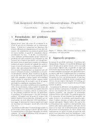
Il procedimento dell’UKF consta di tre passaggi. Nel primo la variabile casuale x viene
approssimata da 2N + 1 punti vi pesati da dei pesi wi scelti in modo tale che media e
varianza coicidano con quelle originali di x. Nel secondo passo si mappano questi punti
attraverso la funzione non lineare g(x). Infine i punti mappati vengono approssimati con un
opportuna gaussiana.
Si ha:
px(·) ∼ N(¯x, Px) y = g(x)
e si approssima la py con una gaussiana ottenendo:
λ u
i i
py(·) ≃ N(¯y, Py)
g(x)
Figura 23.1. Procedimento dell’Unscented Kalman Filter
23-1
media pesata
vazianza

PSC Lezione 23 — 07 Dicembre I Sem. 2010
1. Da px(·) ∼ N(¯x, Px) si generano 2N + 1 punti (dove x ∈ R N ) nel modo seguente:
• v0 = ¯x
• v1 = ¯x + ασ1
• v2 = ¯x − ασ1
.
• v2N−1 = ¯x + ασN
• v2N = ¯x − ασN
dove α è un fattore di scala che viene imposto in modo che la media campionaria dei vi
risulti pari a ¯x e la varianza campionaria degli vi pari a Px. Il calcolo di α si comincia
fattorizzando la varianza di x Px = UDU T , con U = [u1, . . .,uN] una matrice di vettori
ui ortonormali e D la matrice diagonale
⎡ ⎤
D =
⎢
⎣
λ1
Si puó scrivere la Px nel modo seguente:
Px = UDU T
⎡
= ⎢
u1 . . . uN ⎣
√ λ1
. ..
λN
. ..
⎥⎢
⎦⎣
√λN
⎥
⎦ ≥ 0
⎤⎡
= √ λ1u1 . . . √ ⎡ √
λ1u
⎢
λNuN ⎣
T 1
√
.
λNuT ⎤
⎥
⎦
N
= λ1u1u T 1 + . . . + λNuNu T N .
√ λ1
⎤⎡
u T 1
. ..
⎥⎢
⎦⎣
.
√λN
Chiamando σi = √ λiui (vedi vettore rosso in Figura 23.1) si ha che Px = N
i=1 σiσ T i .
La densitá di probabilitá di x puó essere approssimata nel modo seguente:
con i pesi
px(·) ≃
2N
i=0
wiδ(x − vi) = ˆpx(·)
w1 = w2 = . . . = w2N =
w0 = 1 −
2N
i=1
wi = 1 − N
N + κ
23-2
1
2(N + κ)
= κ
N + κ .
u T N
⎤
⎥
⎦

PSC Lezione 23 — 07 Dicembre I Sem. 2010
Vengono ora calcolate la media e la varianza di x relative alla densitá di probablitá
approssimata:
Eˆpx[x] =
2N
x i=0
xwiδ(x − vi)dx =
V arˆpx(x) = Eˆpx[(x − ¯x)(x − ¯x) T
] =
=
ξ
2N
i=0
= α2
N + κ
2N
i=0
2N
x i=0
ξξ T wiδ(ξ + ¯x − vi)dξ =
N
i=1
σiσ T i
= α2
N + κ Px
wivi = ¯x
2N
i=0
wi = ¯x
(x − ¯x)(x − ¯x) T wiδ(x − vi)dx,
N
i=1
1
2(N + κ) 2α2 σiσ T i
avendo effettuato il cambio di variabili ξ = x − ¯x. Poiché si vuole imporre che
V arˆpx(x) = Px si determina α = √ N + κ.
2. Al secondo passo si devono mappare le vi usando la funzione non lineare g(·) ottenendo
così yi = g(vi) con i = 0, . . ., 2N. La densitá di probabilitá approssimata di y risulta
essere
py(·) ≃
2N
i=0
wiδ(y − yi) = ˆpy(·)
3. Al terzo passo si effettuano le seguenti approssimazioni:
ˆpy(·) = N(¯y, Py) ∼ = ˆpy(·), ¯y := Eˆpy[y] =
Py := V arˆpy(y) = Eˆpy[(y − ¯y)(y − ¯y) T ] =
2N
wiyi
i=0
N
wi(y − ¯y)(y − ¯y) T ≥ 0
Tutti i tre passaggi precedenti dovrebbero garantire, almeno sotto opportune ipotesi,
che
ˆpy(·) ∼ = py(·) .
23.1.2 Filtro di Kalman Unscented
Fino ad ora si sono mappate densità di probabilità in densità di probabilità e le abbiamo
approssimate con delle gaussiane.
x µx Px Pxy
∼ N( , )
y
µy
23-3
P T xy Py
i=0

PSC Lezione 23 — 07 Dicembre I Sem. 2010
con
Pxy = cov(x, y) ∼ =
N
wi(vi − ¯x)(yi − ¯y) T
i=1
x|y ∼ N(µx + PxyP −1
y (y − µy), Px − PxyP −1
y P T xy )
Si cerca ora di applicare quanto visto al modello dinamico non lineare:
xk+1 = f(xk, uk, wk)
yk = h(xk, vk)
Non essendo necessariamente wk e vk gaussiani questi vengono approssimati nel modo seguente:
wk ∼ pw(·) ∼ = N( ¯w, Pw)
e dunque si può scrivere y = g(ξ) con
⎡
ξ = ⎣
xk
wk
vk
⎤ ⎡ ⎤
ˆxk|k
⎦ ∼ N( ⎣ ¯w ⎦,
¯v
vk ∼ pv(·) ∼ = N(¯v, Pv)
xk ∼ = N(ˆxk|k, Pk|k)
xk ⊥vk ⊥wk
⎡ ⎤
Pk|k 0 0
⎣ ⎦) ,
0 Pw 0
0 0 Pv
⎧
⎪⎨
⎪⎩
x ∈ R n
y ∈ R m
w ∈ R p
v ∈ R q
ξ ∈ R n+p+q = R N
Si dovranno dunque generare 2N + 1 punti vi = 0, 1, . . ., 2N con i pesi
1
wi =
2(N + κ)
w0 = κ
N + κ .
i = 0
E ora per calcolare ˆxk+1|k+1 ho bisogno di ˆxk+1|k, ˆyk+1|k, P x y xy
k+1|k , Pk+1|k , Pk+1|k , infatti:
ˆxk+1|k+1 = ˆxk+1|k − P xy y
k+1|k (Pk+1|k )−1 (yk+1 − ˆyk+1|k) (23.1)
23-4

PSC Lezione 23 — 07 Dicembre I Sem. 2010
e calcolando:
ˆxk+1|k =
2N
i=0
P x k+1|k =
2N
wif(v x i , u x k, w w i )
wi(f(v x i , uk, w w i ) − ˆxk+1|k)(f(v x i , uk, w w i
i=0
2N
ˆyk+1|k = wih(ˆx i k+1|k , vv i )
P y
k+1|k =
P xy
k+1|k =
i=0
2N
wi(ˆy i k+1|k − ˆyk+1|k)(ˆy i k+1|k − ˆyk+1|k) T
i=0
2N
wi(ˆx i k+1|k − ˆxk+1|k)(ˆy i T
k+1|k − ˆyk+1|k)
i=0
) − ˆxk+1|k) T
si hanno tutti i termini necessari per implementare la (23.1).
Si noti come in questo caso non è necessario linearizzare ad ogni passo la matrice come
nel caso del filtro esteso e si approssimano distribuzioni piuttosto che non linearità. Inoltre
con questo metodo si ottiene una precisione del secondo ordine senza calcolare hessiani o
jacobiani. I pesi possono poi essere scelti in modo tale da catturare statistiche di ordine più
elevato.
Tuttavia nell’implementazione UKF si rende necessario diagonalizzare la matrice di varianza
di ξ al variare di Pk|k. Per rendere meno oneroso questo calcolo si può usare la Squared
UKF (che utilizza la fattorizzazione di Cholesky), chiamando Q fattorizzazione di Cholesky
di P si può scrivere:
⎡ ⎤
v T 1
P = QQ T = ⎢
v1 . . . vN ⎣ .
v T N
⎥
⎦ =
dove Q è triangolare e risulta numericamente più facile da calcolare rispetto alla diagonalizzazione
di P tramite la decomposizione ai valori singolari (SVD).
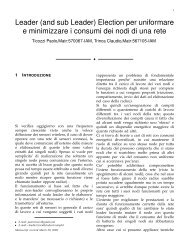
23.2 Confronto tra UKF e EKF: esempio scalare
Si consideri la seguente mappa lineare, che mappa una v.a. gaussiana in un’altra v.a.:
y = x 2 , x ∈ R, x ∼ N(¯x, σ 2 x )
23-5
N
i=0
viv T i

PSC Lezione 23 — 07 Dicembre I Sem. 2010
p
x
x
σ 2
x
x
g(.)=(.) 2
Figura 23.2. Procedimento del filtro UKF
Rappresentando x come x := ¯x+δx con δx ∼ N(0, σ2 x ) si calcolano la media e la varianza
esatta di y:
¯yT = Ey[y] = Ex[x 2 ] = Ex[(¯x + δx) 2 ]
= E[¯x 2 + 2¯xδx + (δx) 2 ]
= ¯x 2 + σ 2 x
(σ 2 y)T = V ar(y) = E[(x 2 − (¯x 2 + σ 2 x) 2 ) 2 ]
= E[4¯x 2 (δx) + (δx) 4 + σ 4 x + 4¯x(δx) 3 − 4¯xσ 2 xδx − 2(δx) 2 σ 2 x]
= 4¯x 2 σ 2 x + E[(δx) 4 ] + σ 4 x − 2σ 4 x
= 2σ 4 x + 4¯x2 σ 2 x
dove nell’ultimo passaggio si è sfruttato il fatto che E[(δx) 4 ] = 3σ4 x . L’esempio prosegue
nella prossima lezione.
23-6
p
y
y

Bibliografia
[1] Giorgio Picci. Fitraggio Statistico (Wiener, Levinson, Kalman) e Applicazioni. Libreria
Progetto, 2006.
[2] J. Uhlmann S. Julier. A general method for approximating nonlinear transformations of
probability distributions. Technical report, University of Oxford, 1996.
[3] E. Wan R. van der Merwe. Sigma-point kalman filters for integrated navigation.
Proceedings of the 60th Annual of the Institute of Navigation, 2004.
[4] G. Oriolo P. Peliti T. Fiorenzani, C. Manes. Comparative study of unscented kalman
filter and extended kalman filter for position/attitude estimation in unmanned aerial
vehicles. Technical report, IASI CNR, 2002.
7