Grafici in matlab Un esempio di grafico:
Grafici in matlab Un esempio di grafico:
Grafici in matlab Un esempio di grafico:

Create successful ePaper yourself
Turn your PDF publications into a flip-book with our unique Google optimized e-Paper software.
1<br />
3<br />
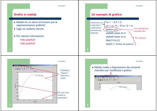
<strong>Grafici</strong> <strong>in</strong> <strong>matlab</strong><br />
Matlab ha un sacco <strong>di</strong> funzioni per le<br />
rappresentazioni grafiche!<br />
Oggi ne ve<strong>di</strong>amo alcune.<br />
Per ulteriori <strong>in</strong>formazioni:<br />
help graph2d<br />
help graph3d<br />
lab10(grafici)<br />
lab10(grafici)<br />
Il default è<br />
“figure1”,<br />
l<strong>in</strong>ea blu e<br />
sottile<br />
Gli assi sono<br />
scalati <strong>in</strong><br />
automatico<br />
2<br />
4<br />
<strong>Un</strong> <strong>esempio</strong> <strong>di</strong> <strong>grafico</strong>:<br />
Notazione con<br />
l’operatore “:”<br />
e operazioni<br />
elemento per<br />
elemento<br />
xv = –3:0.1:3;<br />
yv = xv.^3 – 5*xv.^2 + 4;<br />
plot(xv,yv)<br />
xlabel('value of x')<br />
ylabel('value of y')<br />
title(TITOLO')<br />
text(0,1, Scritta nel <strong>grafico</strong>')<br />
lab10(grafici)<br />
Uso standard del<br />
comando plot<br />
Per annotare<br />
lab10(grafici)<br />
Matlab mette a <strong>di</strong>sposizione dei coman<strong>di</strong><br />
<strong>in</strong>terattivi per mo<strong>di</strong>ficare il <strong>grafico</strong>
5<br />
7<br />
Click sulla freccia per mo<strong>di</strong>ficare<br />
lab10(grafici)<br />
Click destro -> properties su una parte della figura per mo<strong>di</strong>ficarla<br />
In pratica, il property e<strong>di</strong>tor è simile agli<br />
strumenti <strong>di</strong> excel però...<br />
– È limitato ad una s<strong>in</strong>gola figura<br />
– Ripeterlo per ogni nuovo <strong>grafico</strong> è noioso<br />
lab10(grafici)<br />
La funzione plot mette a <strong>di</strong>sposizione degli<br />
argomenti ad<strong>di</strong>zionali per mo<strong>di</strong>ficare da riga<br />
<strong>di</strong> comando:<br />
plot(x,y, 'l<strong>in</strong>espec' , 'Propname' , PropValue )<br />
– Specifiche <strong>di</strong> l<strong>in</strong>ea: colore, tipo <strong>di</strong> l<strong>in</strong>ea, punti dei<br />
dati<br />
– Proprietà e valore: spessore, <strong>di</strong>mensione ecc.<br />
6<br />
8<br />
O anche le l<strong>in</strong>ee:<br />
Specifiche <strong>di</strong> L<strong>in</strong>ea<br />
plot(x,y, ' r : d ' )<br />
rosso<br />
punteggiata<br />
Rombi<br />
(<strong>di</strong>amonds)<br />
lab10(grafici)<br />
lab10(grafici)
9<br />
11<br />
lab10(grafici)<br />
Forma Generale: plot(x,y, '  ')<br />
Colore:<br />
k black<br />
r red<br />
b blue<br />
g green<br />
y yellow<br />
c cyan<br />
w white<br />
m magenta<br />
Simbolo:<br />
. po<strong>in</strong>t<br />
o circle<br />
x x-mark<br />
s square<br />
d <strong>di</strong>amond<br />
Etc ( +, * ,<br />
^ , > , <<br />
,v, p,h).<br />
Tipo L<strong>in</strong>ea:<br />
- solid<br />
: dotted<br />
-- dashed<br />
-. dash-dot<br />
L’ord<strong>in</strong>e non è<br />
importante!<br />
lab10(grafici)<br />
Forma Generale: plot(x,y, '',value)<br />
Proprietà:<br />
l<strong>in</strong>ewidth<br />
markersize<br />
markeredgecolor<br />
markerfacecolor<br />
Valore: <strong>di</strong>pende dalla proprietà<br />
Dimensioni <strong>in</strong> punti<br />
Colori<br />
Possono esserci<br />
coppie multiple !<br />
10<br />
12<br />
Proprietà e valori<br />
plot(x,y, 'l<strong>in</strong>ewidth',5 )<br />
Lo spessore<br />
della l<strong>in</strong>ea è<br />
5 punti<br />
Esempio:<br />
lab10(grafici)<br />
lab10(grafici)<br />
plot(x,y, '- k o' , 'L<strong>in</strong>eWidth' , 3 , 'MarkerSize', 6,…<br />
'MarkerEdgeColor','red','MarkerFaceColor','green')
13<br />
15<br />
Più grafici negli stessi assi<br />
Possiamo <strong>di</strong>segnare<br />
<strong>di</strong>versi grafici sugli<br />
stessi assi:<br />
I colori cambiano…<br />
Possiamo usare hold<br />
per “congelare” il<br />
<strong>grafico</strong><br />
Notare i colori adesso!<br />
lab10(grafici)<br />
lab10(grafici)<br />
14<br />
16<br />
Attenzione…<br />
Se passiamo delle matrici:<br />
plot(x_matrice, y_matrice)<br />
– Grafico colonna per colonna<br />
– Cambia i colori ogni volta<br />
Per un argomento s<strong>in</strong>golo, plot(x):<br />
– Reale/immag<strong>in</strong>ario se x è complesso<br />
– x/<strong>in</strong><strong>di</strong>ce se x è reale<br />
lab10(grafici)<br />
lab10(grafici)
17<br />
19<br />
Altri due coman<strong>di</strong> utili<br />
figure<br />
– Da solo apre una nuova f<strong>in</strong>estra<br />
– figure(n) ci porta alla f<strong>in</strong>estra n-esima<br />
g<strong>in</strong>put(1)<br />
– Crea un mir<strong>in</strong>o sulla figura<br />
lab10(grafici)<br />
– restituisce la posizione (x,y) al click del mouse<br />
– g<strong>in</strong>put(n) restituisce n coppie <strong>di</strong> coord<strong>in</strong>ate<br />
lab10(grafici)<br />
18<br />
20<br />
Aggiungere del testo<br />
Conosciamo già:<br />
– xlabel( 'str<strong>in</strong>g' )<br />
– ylabel( 'str<strong>in</strong>g' )<br />
– title( 'str<strong>in</strong>g' )<br />
– text( x, y, 'str<strong>in</strong>g' )<br />
In più:<br />
– gtext( 'str<strong>in</strong>g' ) – controllato dal puntatore<br />
– legend( 'str<strong>in</strong>g1', … 'str<strong>in</strong>gn', loc)<br />
Ci sono lettere greche, apici e pe<strong>di</strong>ci<br />
Es. gtext( '\beta_1 x^2' )<br />
lab10(grafici)<br />
lab10(grafici)
21<br />
23<br />
lab10(grafici)<br />
E possimao mo<strong>di</strong>ficare l’aspetto del testo<br />
Es.<br />
Es.<br />
gtext( 'cos<strong>in</strong>e' , 'fontsize', 20, 'rotation', 45,<br />
'color' , 'red', )<br />
lab10(grafici)<br />
22<br />
24<br />
Gli assi<br />
Possiamo aggiungere una griglia<br />
grid<br />
O settare i limiti degli assi:<br />
axis( [ xm<strong>in</strong> xmax ym<strong>in</strong> ymax ] )<br />
Possiamo fare dei<br />
grafici logaritmici:<br />
semilogx(x,y)<br />
semilogy(x,y)<br />
loglog(x,y)<br />
I dati negativi<br />
vengono ignorati<br />
lab10(grafici)<br />
lab10(grafici)
25<br />
27<br />
Figure Files<br />
Save per salvare il file .fig<br />
Subplot: una figura, più assi<br />
subplot(2,2,1)<br />
plot(x1,y1)<br />
subplot(2,2,2)<br />
etc.<br />
I parametri sono:<br />
numero <strong>di</strong> righe,<br />
niumero <strong>di</strong> colonne,<br />
settore scelto<br />
lab10(grafici)<br />
lab10(grafici)<br />
26<br />
28<br />
Per esportare le figure<br />
lab10(grafici)<br />
Stampare: Copia (per <strong>in</strong>collare)<br />
Altri tipi <strong>di</strong> grafici 2-D - Polari<br />
x = 1:100;<br />
r = log10(x);<br />
t = x/10;<br />
polar( t, r )<br />
Angolo <strong>in</strong> ra<strong>di</strong>anti<br />
Ampiezza<br />
150<br />
210<br />
120<br />
240<br />
90<br />
270<br />
1<br />
0.5<br />
2<br />
1.5<br />
60<br />
300<br />
lab10(grafici)<br />
180 0<br />
30<br />
330
29<br />
31<br />
lab10(grafici)<br />
Vertical and horizontal bar plots, stem and<br />
stair plots, pie and compass plots:<br />
1<br />
0.9<br />
0.8<br />
0.7<br />
0.6<br />
0.5<br />
0.4<br />
0.3<br />
0.2<br />
0.1<br />
0<br />
-1.5 -1 -0.5 0 0.5 1 1.5<br />
1.5<br />
1<br />
0.5<br />
0<br />
-0.5<br />
-1<br />
-1.5<br />
0 0.1 0.2 0.3 0.4 0.5 0.6 0.7 0.8 0.9 1<br />
Inoltre…<br />
1<br />
0.9<br />
0.8<br />
0.7<br />
0.6<br />
0.5<br />
0.4<br />
0.3<br />
0.2<br />
0.1<br />
0<br />
-1 -0.8 -0.6 -0.4 -0.2 0 0.2 0.4 0.6 0.8 1<br />
1<br />
0.9<br />
0.8<br />
0.7<br />
0.6<br />
0.5<br />
0.4<br />
0.3<br />
-1 -0.8 -0.6 -0.4 -0.2 0 0.2 0.4 0.6 0.8 1<br />
18%<br />
150<br />
210<br />
120<br />
240<br />
14%<br />
23%<br />
90<br />
270<br />
1<br />
0.5<br />
1.5<br />
9%<br />
180 0<br />
lab10(grafici)<br />
Specifiche <strong>di</strong> l<strong>in</strong>ea, proprietà, assi, griglie…<br />
funzionano con gran parte dei tipi <strong>di</strong> <strong>grafico</strong><br />
Molti <strong>di</strong> questi strumenti hanno funzioni<br />
extra… usate l’ help!!!<br />
Possiamo anche fare dei grafici 3-D!<br />
60<br />
300<br />
30<br />
330<br />
36%<br />
30<br />
32<br />
Istogrammi:<br />
40<br />
30<br />
20<br />
10<br />
0<br />
1<br />
0.5<br />
0<br />
-0.5<br />
-1<br />
-1<br />
1<br />
0.5<br />
0<br />
-0.5<br />
-1<br />
2<br />
1<br />
-0.5<br />
0<br />
0<br />
-1<br />
0.5<br />
-2<br />
-2<br />
40<br />
20<br />
0<br />
-1<br />
1<br />
-0.5<br />
-1<br />
0<br />
0<br />
0.5<br />
1<br />
1<br />
1<br />
2<br />
lab10(grafici)<br />
lab10(grafici)<br />
0.5<br />
0<br />
-0.5<br />
-1
33<br />
35<br />
<strong>Grafici</strong> 3-D<br />
Per tracciare una l<strong>in</strong>ea ( x,y,z=f(t) ) <strong>in</strong> un<br />
<strong>di</strong>agramma tri<strong>di</strong>mensionale usiamo la<br />
plot3:<br />
lab10(grafici)<br />
>>t = [0:pi/50:10*pi];<br />
>>plot3(exp(-0.05*t).*s<strong>in</strong>(t),...<br />
exp(-0.05*t).*cos(t),t),...<br />
xlabel(’x’),ylabel(’y’),zlabel(’z’),grid<br />
Superfici<br />
Funzione z = xe −[(x−y2 ) 2 +y 2 ] ,<br />
per −2 ≤ x ≤ 2 and −2 ≤ y ≤ 2, con <strong>in</strong>tervallo 0.1.<br />
lab10(grafici)<br />
>>[X,Y] = meshgrid(-2:0.1:2);<br />
>>Z = X.*exp(-((X-Y.^2).^2+Y.^2));<br />
>>mesh(X,Y,Z),xlabel(’x’),ylabel(’y’),...<br />
zlabel(’z’)<br />
34<br />
36<br />
La curva x = e -0.05t s<strong>in</strong> t, y = e -0.05t cos t, z = t ,<br />
<strong>di</strong>segnata con plot3<br />
Funzione z = xe −[(x−y2 ) 2 +y 2 ]<br />
lab10(grafici)<br />
lab10(grafici)
37<br />
39<br />
Disegno dei contorni<br />
>>[X,Y] = meshgrid(-2:0.1:2);<br />
>>Z = X.*exp(-((X- Y.^2).^2+Y.^2));<br />
>>contour(X,Y,Z),xlabel(’x’),ylabel(’y’)<br />
lab10(grafici)<br />
lab10(grafici)<br />
4 varianti per z = = xe−(x2 +y2 ) : meshc, meshz, and waterfall.<br />
a) mesh, b) meshc, c) meshz, d) waterfall<br />
38<br />
40<br />
Funzione<br />
contour(x,y,z)<br />
mesh(x,y,z)<br />
meshc(x,y,z)<br />
meshz(x,y,z)<br />
surf(x,y,z)<br />
surfc(x,y,z)<br />
lab10(grafici)<br />
[X,Y] = meshgrid(x,y) Crea le matrici X e Y dai vettori x e y per def<strong>in</strong>ire la griglia<br />
[X,Y] = meshgrid(x)<br />
waterfall(x,y,z)<br />
Ancora…<br />
Descrizione<br />
Contorni.<br />
Superficie 3D (griglia).<br />
Come mesh ma con i contorni sotto.<br />
Come mesh ma <strong>di</strong>segna l<strong>in</strong>ee verticali ai bor<strong>di</strong><br />
Superficie sfumata 3D.<br />
Come surf ma con i contorni.<br />
Come [X,Y]= meshgrid(x,x).<br />
Come mesh ma <strong>di</strong>segna l<strong>in</strong>ee solo <strong>in</strong> una <strong>di</strong>rezione.<br />
– Manipolare i grafici (set) …<br />
lab10(grafici)
41<br />
– GUIs – <strong>in</strong>terfacce <strong>di</strong> alto livello<br />
lab10(grafici)