Raddoppio di condotta con distribuzione uniforme di portata - Nettuno

COSTRUZIONI IDRAULICHE
Esercitazione n° 3
A cura del Prof. Giuseppe Del Giudice
In riferimento alla lezione n. 27: Richiami d’idraulica delle condotte in pressione
NETWORK NETTUNO 1
Prof. Giacomo Rasulo
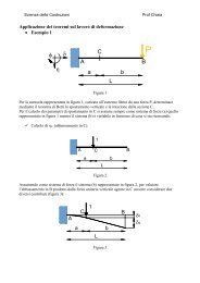
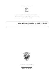
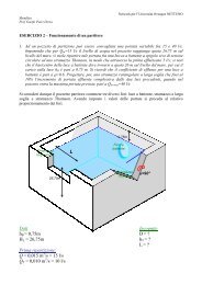
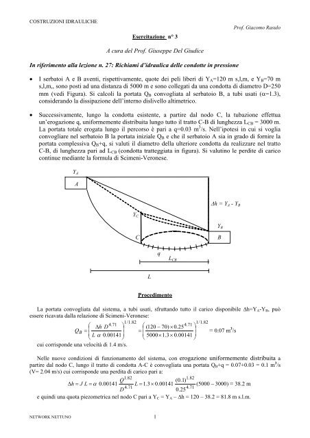
• I serbatoi A e B aventi, rispettivamente, quote dei peli liberi di YA=120 m s,l,m, e YB=70 m
s,l,m,, sono posti ad una distanza di 5000 m e sono collegati da una condotta di diametro D=250
mm (vedi Figura). Si calcoli la portata QB convogliata al serbatoio B, a tubi usati (α=1.3),
considerando la dissipazione dell’interno dislivello altimetrico.
• Successivamente, lungo la condotta esistente, a partire dal nodo C, la tubazione effettua
un’erogazione q, uniformemente distribuita lungo tutto il tratto C-B di lunghezza LCB = 3000 m.
La portata totale erogata lungo il percorso è pari a q=0.03 m 3 /s. Nell’ipotesi in cui si voglia
convogliare nel serbatoio B la portata iniziale QB e che il serbatoio A sia in grado di fornire la
portata complessiva QB+q, si valuti il diametro della ulteriore condotta da realizzare nel tratto
C-B, di lunghezza pari ad LCB (condotta tratteggiata in figura). Si valutino le perdite di carico
continue mediante la formula di Scimeni-Veronese.
YA
A
YC
C
L
q
Procedimento
LCB
Δh = YA - YB
La portata convogliata dal sistema, a tubi usati, sfruttando tutto il carico disponibile Δh=YA-YB, può
essere ricavata dalla relazione di Scimeni-Veronese:
1/
1.
82
1/
1.
82
4.
71
4.
71
( 120 70)
0.
25
0.
00141 5000 1.
3 0.
00141 ⎟ ⎟
⎛ ⎞ ⎛
⎞
⎜ Δh
D
⎜ − ×
Q ⎟
B =
=
= 0.07 m
⎜
⎟ ⎜
⎝
L α
⎠ ⎝
× ×
⎠
3 /s
cui corrisponde una velocità di 1.4 m/s.
Nelle nuove condizioni di funzionamento del sistema, con erogazione uniformemente distribuita a
partire dal nodo C, lungo il tratto di condotta A-C è convogliata una portata QB+q = 0.07+0.03 = 0.1 m 3 /s
(V= 2.04 m/s) cui corrisponde una perdita di carico pari a:
1.
82
1.
82
Q
( 0.
1)
Δh = J L = α 0.
00141 L = 1.
3×
0.
00141 ( 5000 − 3000)
= 38.2 m
4.
71
4.
71
D
0.
25
e quindi una quota piezometrica nel nodo C pari a YC = YA – Δh = 120 – 38.2 = 81.8 m s.l.m.
YB
B

COSTRUZIONI IDRAULICHE
NETWORK NETTUNO 2
Prof. Giacomo Rasulo
La perdita di carico tra i due nodi C e B, uguale per le condotte in parallelo, è YC - YB = 81.8 – 70 = 11.8
m.
La ripartizione della portata complessiva QB+q tra i due rami paralleli è tale che nel ramo inferiore
(esistente) si immette, in testa, la portata Q1 mentre nel ramo superiore (di progetto) è convogliata la portata
Q2. L’equazione di continuità nel nodo C è quindi:
QB + q = Q1
+ Q2
= 0.1 m 3 /s
Analogamente, tenuto conto che la portata q è distribuita lungo tutto il ramo inferiore (esistente), nel nodo
B arriverà:, dal tratto superiore (di progetto), la portata Q2 e dal tratto inferiore (esistente) la portata Q1-q =
Qu. L’equazione di continuità nel nodo B è quindi:
Q = Q2
+ Q = 0.07 m 3 /s
B
La portata Qu può essere calcolata mediante l’equazione del moto (Scimeni-Veronese), applicata al tratto
inferiore con erogazione distribuita, facendo riferimento alla portata equivalente Qeq = Qu+0.56 q.
Q eq
⎛ 4.
71 ⎞
⎜ Δh
D
=
⎟
⎜ 0.
00141⎟
⎝
L α
⎠
1/
1.
82
u
⎛
⎜ 11.
8 × 0.
25
=
⎜
⎝
3000 × 1.
3×
4
. 71
0.
00141
⎟ ⎟
⎞
⎠
1/
1.
82
= 0.042 m 3 /s
Nota Qeq , la portata uscente Qu sarà ricavata dalla relazione Qu = Qeq-0.56 q, da cui Qu = 0.042 - 0.56 x
0.03 = 0.025 m 3 /s.
Applicando l’equazione di continuità al nodo B è possibile ricavare la portata Q2 relativa al ramo
superiore:
Q = 0.
07 − 0.
025 = 0.045 m 3 /s
2
Applicando la relazione del moto al tratto superiore è possibile ricavare il diametro teorico della
tubazione di progetto D*:
1.
82
1/
4.
71
1.
82
1/
4.
71
0.
045
* 0. 00141
1.
3 0.
00141 3000
11.
8 ⎟ ⎛ Q ⎞ ⎛
⎞
D = ⎜
⎜α
L ⎟ = ⎜ ×
= 0.256 m = 256 mm
⎝
Δh
⎠ ⎝
⎠
Occorre scegliere quindi il diametro commerciale immediatamente superiore a quello teorico ricavato
dissipando il carico esuberante mediante una opportuna strozzatura (saracinesca) collocata lungo la condotta
di progetto.