Scarica la tesi Integrale di Feynman sui Cammini e Processi Stocastici

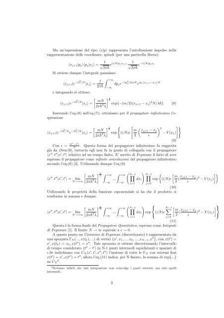
Ma un’espressione del tipo 〈x|p〉 rappresenta l’autofunzione impulso nella
rappresentazione delle coordinate, quindi (per una particella libera):
〈xj+1|pj〉〈pj|xj〉 = 1
√ e
2π¯h (i/¯h)pjxj+1 1
√2π¯h e −(i/¯h)pjxj
Si ottiene dunque l’integrale gaussiano
〈xj+1|e −λT /N |xj〉 = 1
2π¯h
e integrando si ottiene:
〈xj+1|e −λT /N |xj〉 =
mN
2π¯h 2 λ
+∞
−∞
dpje −λp2
j /2mN e ipj(xj+1−xj)/¯h
1
2
exp{−(m/2)(xj+1 − xj) 2 N/λ¯h} (8)
Inserendo l’eq.(8) nell’eq.(7), otteniamo per il propagatore infinitesimo l’espressione
〈xj+1|e −λT /N e −λV /N |xj〉 =
1
2
m
exp (i/¯h)ɛ
2
mN
2π¯h 2 λ
2
xj+1 − xj
− V (xj)
ɛ
(9)
Con ɛ = (t′′ −t ′ )
. Questa forma del propagatore infinitesimo fu suggerita
N
già da Dirac[6], tuttavia egli non fu in grado di collegarla con il propagatore
〈x ′′ , t ′′ |x ′ , t ′ 〉 relativo ad un tempo finito. E’ merito di Feynman il fatto di aver
espresso il propagatore come infinite convoluzioni del propagatore infinitesimo
secondo l’eq.(6) [2]. Utilizzando dunque l’eq.(9)
〈x ′′ , t ′′ |x ′ , t ′
mN
〉 = lim
N→+∞ 2π¯h 2 N
2
λ
+∞
...
−∞
+∞
−∞
N−1
i=1
dxi
N−1
j=0
m
exp (i/¯h)ɛ
(10)
Utilizzando le proprietà della funzione esponenziale si ha che il prodotto si
trasforma in somma e dunque
〈x ′′ , t ′′ |x ′ , t ′
mN
〉 = lim
N→+∞ 2π¯h 2 N
2
λ
+∞
...
−∞
+∞
−∞
⎧
N−1 ⎨
dxi exp
⎩ (i/¯h)ɛ
N−1
m
(11)
Questa è la forma finale del Propagatore Quantistico, espresso come Integrale
di Feynman [1]. Il limite N → ∞ equivale a ɛ → 0.
A questo punto un Cammino di Feynman (discretizzato) è rappresentato da
una spezzata ΓN(..., x(tk), ...) di vertici {x ′ , x1, ..., xk, ..., xN−1, x ′′ }, con x(t ′ ) =
x ′ , x(tk) = xk, x(t ′′ ) = x ′′ . Tale spezzata si ottiene discretizzando l’intervallo
di tempo considerato (t ′′ − t ′ ) in N-1 punti intermedi equidistanti e spaziati di
ɛ.Se indichiamo con CN (x ′ , t ′ ; x ′′ , t ′′ ) l’insieme di tutte le ΓN con estremi fissi
x(t ′ ) = x ′ , x(t ′′ ) = t ′′ , allora l’eq.(11) indica, per N fissato, la somma di exp{...}
su CN 2 .
2 Notiamo infatti che tale integrazione non coinvolge i punti estremi, ma solo quelli
intermedi.
3
i=1
j=0
2 (xj+1 − xj
)
ɛ
2 − V (xj)
2 (xj+1 − xj
)
ɛ
2 − V (xj)
⎫ ⎬
⎭