Scarica la tesi Integrale di Feynman sui Cammini e Processi Stocastici
Scarica la tesi Integrale di Feynman sui Cammini e Processi Stocastici
Scarica la tesi Integrale di Feynman sui Cammini e Processi Stocastici

Create successful ePaper yourself
Turn your PDF publications into a flip-book with our unique Google optimized e-Paper software.
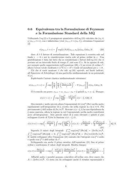
0.6 Equivalenza tra <strong>la</strong> Formu<strong>la</strong>zione <strong>di</strong> <strong>Feynman</strong><br />
e <strong>la</strong> Formu<strong>la</strong>zione Standard del<strong>la</strong> MQ<br />
Utilizzando l’eq.(2) e il propagatore quantistico dell’eq.(13) calco<strong>la</strong>to da (xk, t)<br />
a (xk+1, t + ɛ), con ɛ infini<strong>tesi</strong>mo (cioè 〈xk+1, t + ɛ|xk, t〉), otteniamo l’equazione<br />
[2]:<br />
<br />
ψ(xk+1, t + ɛ) = exp[(i/¯h)S(xk+1, xk)]ψ(xk, t)dxk/A (20)<br />
dove A è il fattore <strong>di</strong> normalizzazione. Tale equazione è corretta solo nel<br />
limite ɛ → 0 e noi <strong>la</strong> considereremo esatta solo al primo or<strong>di</strong>ne in ɛ. Una<br />
giustificazione è data dal fatto che se consideriamo i fattori dell’eq.(11) che ci<br />
portano ad un intervallo finito <strong>di</strong> tempo T , essi sono T/ɛ. Se in ognuno <strong>di</strong> essi,<br />
per esempio quello rappresentato nell’equazione (20), c’è un errore <strong>di</strong> or<strong>di</strong>ne ɛ 2 ,<br />
allora l’errore totale risultante è (ɛ 2 T/ɛ) = ɛT e tende ad annul<strong>la</strong>rsi per ɛ → 0 .<br />
Ciò che si vuole mostrare è che tale eq.(20) equivale, nei limiti in<strong>di</strong>cati,<br />
all’Equazione <strong>di</strong> Schrö<strong>di</strong>nger <strong>di</strong> una particel<strong>la</strong> uni<strong>di</strong>mensionale in un potenziale<br />
V (x).<br />
Esplicitando l’azione c<strong>la</strong>ssica uni<strong>di</strong>mensionale otteniamo:<br />
<br />
2<br />
iɛ m xk+1 − xk<br />
ψ(xk+1, t + ɛ) = exp<br />
− V (xk+1) ψ(xk, t)dxk/A.<br />
¯h 2 ɛ<br />
Ci è comodo ora porre: xk+1 = x, xk+1 −xk = ξ quin<strong>di</strong> xk = x−ξ. Dunque:<br />
<br />
2 imξ iɛV (x)<br />
ψ(x, t + ɛ) = exp − ψ(x − ξ, t)dξ/A<br />
2ɛ¯h ¯h<br />
Ora essendo ɛ molto piccolo allora l’esponenziale <strong>di</strong> (imξ2 /2¯hɛ) oscil<strong>la</strong> molto<br />
rapidamente nell’integrazione <strong>di</strong> ξ, eccetto che nel<strong>la</strong> regione in cui ξ ≈ 0. Più<br />
precisamente ξ dell’or<strong>di</strong>ne <strong>di</strong> (¯hɛ/m) 1<br />
2 . Siccome ψ(x−ξ, t) ha una <strong>di</strong>pendenza da<br />
ξ meno marcata, allora <strong>la</strong> regione in cui l’esponenziale oscil<strong>la</strong> molto contribuirà<br />
poco all’integrazione. Solo piccoli valori <strong>di</strong> ξ sono rilevanti e quin<strong>di</strong> si può<br />
sviluppare il serie <strong>di</strong> Tylor <strong>la</strong> funzione ψ(x − ξ, t):<br />
<br />
iɛV (x)<br />
ψ(x, t+ɛ) = exp −<br />
¯h<br />
2 imξ ∂ψ(x, t) ξ2 ∂<br />
exp · ψ(x, t) − ξ +<br />
2¯hɛ<br />
∂x 2<br />
2ψ(x, t)<br />
∂x2 <br />
− ... dξ/A.<br />
Sapendo il valore degli integrali:<br />
(21)<br />
+∞<br />
−∞ exp(imξ2 /2¯hɛ)dξ = (2πi¯hɛ/m) 1<br />
2 ,<br />
+∞<br />
−∞ exp(imξ2 /2¯hɛ)ξdξ = 0, +∞<br />
−∞ exp(imξ2 /2¯hɛ)ξ 2 dξ = (¯hɛi/m)(2πi¯hɛ/m) 1<br />
2 .<br />
E’ inutile sviluppare oltre l’equazione (21) essendo che l’integrale con ξ 3 è nullo<br />
e quello con ξ 2 è dell’or<strong>di</strong>ne <strong>di</strong> ɛ 2 .<br />
Sviluppando ora anche il primo membro dell’equazione (21) fino al primo<br />
or<strong>di</strong>ne e sostituiamo il valore degli integrali. Risulta dunque:<br />
2<br />
∂ψ(x, t) iɛV (x) (2π¯hiɛ/m)<br />
ψ(x, t)+ɛ = exp − · ψ(x, t) +<br />
∂t<br />
¯h A<br />
¯hɛi<br />
2m<br />
∂ 2 ψ(x, t)<br />
∂x 2<br />
<br />
+ ...<br />
Affinchè ambo i membri possano coincidere all’or<strong>di</strong>ne zero deve essere che<br />
A = (2π¯hɛi/m) 1<br />
2 . Ci resta ora da sviluppare anche il termine esponenziale e<br />
8