Teoria della selezione del portafoglio e modelli di equilibrio del ...

More documents

Recommendations

Info

SIMULAZIONE Determinazione del portafoglio efficiente componendo i tre business B, D, E. (I dati utilizzati si rifanno alle tabelle 2, 3 e 4, arrotondati alla quarta cifra decimale). Si ponga di voler ottenere un rendimento atteso di portafoglio di 15.6. ⎧ n ⎪ n n ∑ xi = 1 ⎪ i= 1 F.O. = min 0.5 VP = min 0.5 ∑∑ xixjσ ij con vincoli ⎨ n i= 1 j= 1 ⎪ * ⎪∑ xR i i = RP ⎩ i= 1 ⎛ 3 ⎞ ⎛ 3 ⎞ * Lx ( i, λS, λR) = 05 . VP + λ ⎜ S⎜ 1−∑x⎟ i⎟ + λ ⎜ R⎜ RP −∑xR⎟ i i⎟ ⎝ ⎠ ⎝ ⎠ i= 1 i= 1 ⎛ σ σ σ ⎞⎛ x ⎞ ⎜ ⎟⎜ ⎟ ⎛ ⎞ ⎛ ⎞ Lx ( i, λS, λR) = . ( x x x) ⎜σ σ σ ⎟⎜ x ⎟ + λ ⎜ S − x ⎟ ⎜ i⎟ + λ ⎜ R RP − xiR ⎟ ⎜ i⎟ ⎜ ⎟⎜ ⎟ σ σ σ x ⎝ ⎝ i ⎠ ⎝ ⎠ i ⎠ ⎝ ⎠ x . [ ( x σ x σ x σ )( x σ x σ x σ )( x σ x σ x σ ) ] x x λ S = ⎛ ⎞ ⎜ ⎟ = + + + + + + ⎜ ⎟ ⎜ ⎟ ⎝ ⎠ + 11 12 13 1 3 3 ∗ 05 1 2 3 21 22 23 2 1 ∑ ∑ = 1 = 1 31 32 33 3 1 05 1 11 2 21 3 31 1 12 2 22 3 32 1 13 2 23 3 33 2 3 ⎛ ⎞ ⎛ ⎞ + ⎜ ∗ 1−∑x ⎟ ⎜ i ⎟ + ⎜ R RP −∑x R ⎟ ⎜ i i⎟ ⎝ i= ⎠ ⎝ i= ⎠ [ x ( x x x ) x ( x x x ) x ( x x x ) ] ∗ S ∑xi R RP ∑xiRi i= i= x x x x x x x x x = = + + + + + + + + + ⎛ ⎞ ⎛ ⎞ + ⎜ − ⎟ + ⎜ − ⎟ ⎜ ⎟ ⎝ ⎠ ⎝ ⎠ = 3 3 λ 1 1 05 . 1 1σ11 2σ213σ31 2 1σ122σ223σ3231σ13 2σ233σ33 3 3 λ 1 λ 1 1 = 05 . σ + σ + σ + σ + σ + x σ + x x σ + x x σ + x σ + =0.5 1 2 11 1 2 21 1 3 31 1 2 12 2 2 ( 22 2 3 32 1 3 13 2 3 23 3 ) S x x x R RP x R x R x R 2 33 + λ 1− 1 − 2 − 3 + λ ∗ − 1 1 − 2 2 − 3 3 = ( ) ( ) per la simmetria delle covarianze si ha: 2 ( x1σ11 2 x2σ22 2 x3σ332x1x2σ12 2x1x3σ13 2x2x3σ23) ∗ + λS( 1− x1 − x2 − x3) + λR( RP − x1R1 − x2R2 − x3R3) = + + + + + + L'ottimo si ha uguagliando a zero le derivate parziali: ⎧ ∂L 1 ⎪ = ( 2x1σ11 + 2x2σ12 + 2x3σ13) −λS − λRR1 = 0 ⎪ ∂x1 2 ⎪ ∂L 1 ⎪ = ( 2x2σ22 + 2x1σ21 + 2x3σ23) −λS − λRR2 = 0 ⎪ ∂x2 2 ⎪ ∂L 1 ⎨ = ( 2x3σ33 + 2x1σ31 + 2x2σ32) −λS − λRR3 = 0 ⎪∂x3 2 ⎪ ∂L ⎪ = 1−x1 − x2 − x3 = 0⇒ x1 + x2 + x3 = 1 ⎪∂λ S ⎪ ∂L ⎪ = R − R1x1− R2x2− R3x3= 0 ⇒ R1x1+ R2x2+ R3x3= R ⎩∂λ R che posto in forma matriciale: ∗ ∗ P P 47
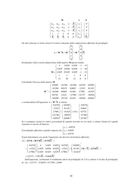
M x b ⎛ σ11 ⎜ ⎜σ21 ⎜σ ⎜ 31 ⎜ 1 ⎜ ⎝ R σ12 σ22 σ32 1 R σ13 σ23 σ33 1 R −1 −1 −1 0 0 −R1⎞⎛x1⎞ ⎛ 0 ⎞ ⎟ ⎜ ⎟ ⎜ ⎟ −R2⎟⎜x2⎟ ⎜ 0 ⎟ −R⎟⎜ 3 x ⎟ 3 = ⎜ 0 ⎟ ⎟ ⎜ ⎟ ⎜ ⎟ 0 ⎟ ⎜ λ S ⎟ ⎜ 1 ⎟ ⎟ ⎜ ⎟ ⎜ ∗⎟ 0 ⎠ ⎝λ ⎠ ⎝ R ⎠ 1 2 3 48 R P Da tale relazione si vuole estrarre il vettore soluzione della composizione efficiente di portafoglio. ⎛0⎞ ⎛0⎞ ⎜ ⎟ ⎜ ⎟ ⎜0⎟ ⎜0⎟ −1 −1 1 x = M b = M ⎜ ⎟ − + M ⎜ ⎟ ∗ 0 0 RP ⎜ ⎟ ⎜ ⎟ ⎜1⎟ ⎜0⎟ ⎜ ⎟ ⎜ ⎟ ⎝0⎠ ⎝1⎠ Sostituendo i dati a nostra disposizione nella matrice M questa risulta: ⎛ 4 ⎜ ⎜11429 . M = ⎜11429 . ⎜ ⎜ 1 ⎜ ⎝ 15 11429 . 34286 . 01429 . 1 20 11429 . 01429 . 11429 . 1 12 −1 −1 −1 0 0 −15⎞ ⎟ −20⎟ −12⎟ ⎟ 0 ⎟ 0 ⎠ Calcolando l'inversa della matrice M: M − ⎛ 0. 3690 ⎜ ⎜ −01384 . 1 = ⎜−0. 2306 ⎜ ⎜ 0. 4745 ⎜ ⎝−0. 0280 −01384 . 0. 0519 0. 0865 13221 . −01145 . −0. 2306 0. 0865 01442 . −2. 7965 01425 . −0. 4745 −13221 . 2. 7965 131757 . −0. 8926 0. 0280 ⎞ ⎟ 01145 . ⎟ −01425 . ⎟ ⎟ −0. 8926 ⎟ 0. 0648 ⎠ 1 − e sostituendola nell'equazione x = M b si ottiene: ⎛−0. 4745⎞ ⎛ 0. 0280 ⎞ ⎛−0. 0376⎞ ⎜ ⎟ ⎜ ⎟ ⎜ ⎟ ⎜ −13221 . ⎟ ⎜ 01145 . ⎟ ⎜ 0. 4641 ⎟ ⎜ 2. 7966 ⎟ + ⎜ −01425 . ⎟ × 15. 6 = ⎜ 0. 5735 ⎟ ⎜ ⎟ ⎜ ⎟ ⎜ ⎟ ⎜ 131746 . ⎟ ⎜−0. 8925⎟ ⎜ −0. 7483⎟ ⎜ ⎟ ⎜ ⎟ ⎜ ⎟ ⎝ −0. 8925⎠ ⎝ 0. 0648 ⎠ ⎝ 01189 . ⎠ Se si sommano i primi tre valori, percentuali di capitale investito nei tre titoli, si ottiene l'unità ed è quindi rispettato il vincolo di bilancio. ⎧x1 =−00376 . ⎪ Il portafoglio efficiente è quindi composto da: ⎨x2 = 0. 4641 ⎪ ⎩x3 = 0. 5735 Si può determinare ora anche l'equazione che descrive la frontiera efficiente: 2 σ P h'Ch ∗ 2k'ChRP ' 2 ∗ k'CkRP = + + = ⎛−0 4745⎞ ⎛ 4 11429 11429⎞ ⎛−0 4745⎞ 0 0280 ⎜ ⎟ ⎜ ⎟⎜ ⎟ 2 = ⎜ −13221⎟ ⎜11429 34286 01429⎟⎜ −13221⎟ 2 01145 RP RP ⎜ ⎟ ⎜ ⎟⎜ ⎟ ⎝ 2 7966 ⎠ ⎝11429 01429 11429⎠ ⎝ 2 7966 ⎠ 01425 + ′ . . . . ⎛ . ⎞ ⎜ ⎟ ∗ ∗ . . . . . ⎜ . ⎟ Ch × + k'Ck = ⎜ ⎟ . . . . . ⎝− . ⎠ 2 ∗ ∗ P P = 131757 . − 17851 . R + 0. 0648R Dall'equazione, sostituendo il rendimento atteso di portafoglio di 15.6 si ottiene il rischio di portafoglio 2 = 131757 . − 27. 8479 + 15. 7790 = 11069 . di: σ P
Page 1 and 2: UNIVERSITÀ DEGLI STUDI DI VERONA D
Page 3 and 4: 5.2.5 Alcune simulazioni della valu
Page 5 and 6: 1 RENDIMENTO E RISCHIO DI UN’ATTI
Page 7 and 8: invece della distribuzione di proba
Page 9 and 10: − E ha il rendimento più basso e
Page 11 and 12: 2 ANALISI DI UN PORTAFOGLIO COMPOST
Page 13 and 14: Si può standardizzare la covarianz
Page 15 and 16: Fig. 2: Un esempio di dispersione c
Page 17 and 18: A) Componendo un portafoglio F ripa
Page 19 and 20: B) Componendo un portafoglio Q ripa
Page 21 and 22: C) Componendo empiricamente un port
Page 23 and 24: x1 + x2 = 1 Il rendimento atteso di
Page 25 and 26: Operando su due business a rendimen
Page 27 and 28: dalla quale risulta evidente che, a
Page 29 and 30: SIMULAZIONI : valutazione del porta
Page 31 and 32: Visto il coefficiente angolare dell
Page 33 and 34: ANALISI DI PORTAFOGLIO CON n TITOLI
Page 35 and 36: 3.2.2 Caso di titoli o business con
Page 37 and 38: titoli, negli Stati Uniti, si può
Page 39 and 40: Tab. 7: Matrice dei coefficienti di
Page 41 and 42: n n ⎧ ⎪min Z3= 0.5 V P = 0.5 xi
Page 43 and 44: Possiamo ora “criticare” il por
Page 45 and 46: B) IN RIFERIMENTO AL CASO IN CUI NO
Page 47 and 48: In conclusione: G è dominato sia n
Page 49: ⎡0⎤ ⎡R 1 ⎤ ⎧x1 = p1 + q1
Page 53 and 54: SIMULAZIONE Determinazione della co
Page 55 and 56: ) Consideriamo il portafoglio xc co
Page 57 and 58: 4 ANALISI DEL PORTAFOGLIO IN PRESEN
Page 59 and 60: n ⎛ ⎞ 1) l'unico vincolo del pr
Page 61 and 62: − investire x U = 0.5/0.82 = 0.61
Page 63 and 64: − rendimento lordo di lire 22.397
Page 65 and 66: ROI, ROE E SOSTENIBILITA' DEI DEBIT
Page 67 and 68: ) l’intensità della leva finanzi
Page 69 and 70: σ(roe) c = 8 U H 66 H E(roe) insie
Page 71 and 72: definita fra un roe atteso di 19 e
Page 73 and 74: 5.2.5 Alcune simulazioni della valu
Page 75 and 76: Fig. 30 si illustrano le relazioni
Page 77 and 78: Il rendimento di portafoglio avrà
Page 79 and 80: 6.1.4. La valutazione delle soluzio
Page 81 and 82: Siano, inoltre: EI ( ) = 161 . = n+
Page 83 and 84: 7 MODELLI SEMPLIFICATI DI SELEZIONE
Page 85 and 86: − la covarianza del rendimento de
Page 87 and 88: ESEMPIO Data l'applicazione lineare
Page 89 and 90: Per semplificazione si tratterà la
Page 91 and 92: determinando λ2 e a2. Dopo p itera
Page 93 and 94: p ∑ λi = i= 1 poichè tale somma
Page 95 and 96: a $x = z a ⎛ 11⎞ ⎜ ⎟ ⎝
Page 97 and 98: A questo punto, pur avendo determin
Page 99 and 100: Anche in Italia si è utilizzato pi
Page 101 and 102:
8 LA SCELTA PREFERITA 8.1 Introduzi
Page 103 and 104:
Come in ambito certo, anche per l'u
Page 105 and 106:
In sintesi, mentre il postulato di
Page 107 and 108:
Ritornando alla Fig. 33, se il sogg
Page 109 and 110:
con i parametri a1 ed a2 costanti t
Page 111 and 112:
ug(x) 100 80 60 40 20 0 0 2 4 6 8 1
Page 113 and 114:
capitale (ricchezza) disponibile se
Page 115 and 116:
Se si considerano la variabile alea
Page 117 and 118:
2 2 2 Allora, data l'equazione dell
Page 119 and 120:
SIMULAZIONI Si consideri la frontie
Page 121 and 122:
118 9 MODELLI DI EQUILIBRIO 9.1. Eq
Page 123 and 124:
Una supposizione iniziale per formu
Page 125 and 126:
Fig. 41: Security Market Line con s
Page 127 and 128:
9.3. L'Arbitrage Pricing Theory (A.
Page 129 and 130:
Per poter raggiungere la specificaz
Page 131 and 132:
dimensione dei futuri flussi di cas
Page 133 and 134:
Rendimento Medio E’ la semplice m
Page 135 and 136:
il suo utilizzo permette di conside
Page 137 and 138:
⎛ RG a − R ⎞ Indice di Sharpe
Page 139 and 140:
β = N ∑ i= 1 Dove: cov β = σ (
Page 141 and 142:
- CONSTANTINIDES G.M., MALLIARIS A.
Page 143 and 144:
- ROSS S. A., "Return Risk and Arbi
show all

Teoria della selezione del portafoglio e modelli di equilibrio del ...

You also want an ePaper? Increase the reach of your titles

Delete template?

Save as template?