THÃS EE - CESBIO - Université Toulouse III - Paul Sabatier
THÃS EE - CESBIO - Université Toulouse III - Paul Sabatier THÃS EE - CESBIO - Université Toulouse III - Paul Sabatier
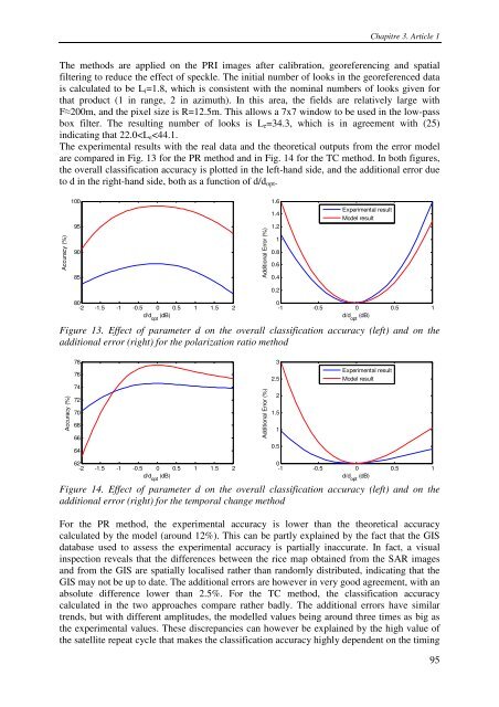
Chapitre 3. Article 1The methods are applied on the PRI images after calibration, georeferencing and spatialfiltering to reduce the effect of speckle. The initial number of looks in the georeferenced datais calculated to be L i =1.8, which is consistent with the nominal numbers of looks given forthat product (1 in range, 2 in azimuth). In this area, the fields are relatively large withF≈200m, and the pixel size is R=12.5m. This allows a 7x7 window to be used in the low-passbox filter. The resulting number of looks is L e =34.3, which is in agreement with (25)indicating that 22.0
Chapitre 3. Article 1of the acquisitions. The calculated value of ∆r TC is therefore not necessarily representative ofthe ∆r 90% parameter, and the assessment of ∆r TC,opt may be incorrect.Based on the results obtained in the PR method, the model can be effectively used to assessthe effects of channel gain imbalance or radiometric stability.B. Sensitivity to ambiguity ratioThe ambiguity is simulated by degrading the SLC images according to the relationship givenin (21), for each polarization and each date, and for five ambiguity ratio values: -5dB, -10dB,-17dB, -20dB and -25dB. The -5dB and -10dB values are not realistic but are neverthelesssimulated to test the sensitivity of the model. Contrarily to the analysis in IV.A. where thesource of the ambiguity is set at a constant backscatter value of 0dB to simulate the worstpossible case, a real scene is selected here from another subset of the image. This is thereforeexpected to produce lower additional errors than the theoretical study.After simulating the ambiguity in the complex amplitude images in slant-range geometry, thebackscattering coefficient is computed, a 3x15 low-pass box-filter is applied to reduce thespeckle while taking into account the different pixel spacing in range and azimuth, and theimages are georeferenced to the GIS geometry using tie-points. The number of looks of thegeoreferenced images is calculated to be L=19.Figure 15 represents the variations of the ∆r parameter and of the additional error due toambiguity as a function of the ambiguity ratio, calculated for the five experimental values andsimulated by the error model for the PR method. The error model is run with p(B)=0.75,L=19, ∆r=6.57dB, and I 1,B =-6dB, which is calculated from the HH and VV images.∆r (dB)8765432Effect of ambiguity on ∆rTheoretical resultsExperimental resultsAdditional error due to ambiguity (%)1098765432Additional error due to ambiguityTheoretical resultsExperimental results10-30 -25 -20 -15 -10 -5Ambiguity ratio (dB)10-30 -25 -20 -15 -10 -5Ambiguity ratio (dB)Figure 15. Effect of ambiguity ratio on the class separability (left) and additional error due toambiguity (right) for the polarization ratio method96
- Page 46 and 47: Chapitre 2. Principes de l’imager
- Page 48 and 49: Chapitre 2. Principes de l’imager
- Page 50 and 51: Chapitre 2. Principes de l’imager
- Page 52 and 53: Chapitre 2. Principes de l’imager
- Page 54 and 55: Chapitre 2. Principes de l’imager
- Page 56 and 57: Chapitre 2. Principes de l’imager
- Page 58 and 59: Chapitre 2. Principes de l’imager
- Page 60 and 61: Chapitre 2. Principes de l’imager
- Page 62 and 63: Chapitre 3. Modèle d’erreur pour
- Page 64 and 65: Chapitre 3. Modèle d’erreur pour
- Page 66 and 67: Chapitre 3. Modèle d’erreur pour
- Page 68 and 69: Chapitre 3. Modèle d’erreur pour
- Page 70 and 71: Chapitre 3. Modèle d’erreur pour
- Page 72 and 73: Chapitre 3. Modèle d’erreur pour
- Page 74 and 75: Chapitre 3. Article 12011, Sentinel
- Page 76 and 77: Chapitre 3. Article 1rrB⎛ p(A)⎞
- Page 78 and 79: Chapitre 3. Article 1- p(B), the a
- Page 80 and 81: Chapitre 3. Article 1imperfections,
- Page 82 and 83: Chapitre 3. Article 11.210.80.60.40
- Page 84 and 85: Chapitre 3. Article 1and p(B)=0.5 (
- Page 86 and 87: Chapitre 3. Article 122∆ 2δShv+
- Page 88 and 89: Chapitre 3. Article 1Additional err
- Page 90 and 91: Chapitre 3. Article 1As suggested i
- Page 92 and 93: Chapitre 3. Article 1Particular val
- Page 94 and 95: Chapitre 3. Article 1Table 1 summar
- Page 98 and 99: Chapitre 3. Article 1As predicted b
- Page 100 and 101: Chapitre 3. Article 1Considering th
- Page 102 and 103: Chapitre 4. Cartographie des riziè
- Page 104 and 105: Chapitre 4. Cartographie des riziè
- Page 106 and 107: Chapitre 4. Cartographie des riziè
- Page 108 and 109: Chapitre 4. Cartographie des riziè
- Page 110 and 111: Chapitre 4. Article 2109
- Page 112 and 113: Chapitre 4. Article 2111
- Page 114 and 115: Chapitre 4. Article 2113
- Page 116 and 117: Chapitre 4. Article 2115
- Page 118 and 119: Chapitre 4. Article 2117
- Page 120 and 121: Chapitre 5. Cartographie des riziè
- Page 122 and 123: Chapitre 5. Cartographie des riziè
- Page 124 and 125: Chapitre 5. Article 3USE OF ENVISAT
- Page 126 and 127: Chapitre 5. Article 3during the rep
- Page 128 and 129: Chapitre 5. Article 3which is plant
- Page 130 and 131: Chapitre 5. Article 3the whole prov
- Page 132 and 133: Chapitre 5. Article 3The 36 VGT-S10
- Page 134 and 135: Chapitre 5. Article 3tTCTCTCTCr⎛
- Page 136 and 137: Chapitre 5. Article 3Figure 7. Rice
- Page 138 and 139: Chapitre 5. Article 3Table 3. Plant
- Page 140 and 141: Chapitre 5. Article 3Table 5. Retri
- Page 142 and 143: Chapitre 5. Article 3Tien GiangMTC
- Page 144 and 145: Chapitre 5. Article 3Le Toan, T., R
Chapitre 3. Article 1The methods are applied on the PRI images after calibration, georeferencing and spatialfiltering to reduce the effect of speckle. The initial number of looks in the georeferenced datais calculated to be L i =1.8, which is consistent with the nominal numbers of looks given forthat product (1 in range, 2 in azimuth). In this area, the fields are relatively large withF≈200m, and the pixel size is R=12.5m. This allows a 7x7 window to be used in the low-passbox filter. The resulting number of looks is L e =34.3, which is in agreement with (25)indicating that 22.0


