Variations spatio-temporelle de la microflore des sols alpins

Variations spatio-temporelle de la microflore des solsalpinsLucie ZingerTo cite this version:Lucie Zinger. Variations spatio-temporelle de la microflore des sols alpins. Ecology, environment.Université Joseph-Fourier - Grenoble I, 2009. French. HAL Id: tel-00421411https://tel.archives-ouvertes.fr/tel-00421411Submitted on 1 Oct 2009HAL is a multi-disciplinary open accessarchive for the deposit and dissemination of scientificresearch documents, whether they are publishedor not. The documents may come fromteaching and research institutions in France orabroad, or from public or private research centers.L’archive ouverte pluridisciplinaire HAL, estdestinée au dépôt et à la diffusion de documentsscientifiques de niveau recherche, publiés ou non,émanant des établissements d’enseignement et derecherche français ou étrangers, des laboratoirespublics ou privés.

UNIVERSITE JOSEPH FOURIER – GRENOBLE I Année 2009Ecole Doctorale Chimie et Sciences du VivantTHESEPour l’obtention du titre deDOCTEUR EN BIOLOGIEMention Biodiversité-Ecologie-EnvironnementVariations spatio-temporelles de la microfloredes sols alpinsPrésentée et soutenue publiquement parLucie ZINGERLe 10 Juillet 2009Composition du jury :Jean-Jacques BRUN – Directeur de recherche, CEMAGREF, Grenoble – ExaminateurChristiane GALLET – Maître de conférences, Université de Savoie – Co-directrice de thèseRoberto GEREMIA – Directeur de recherche, CNRS, Grenoble – Directeur de thèsePhilippe NORMAND – Directeur de recherche, CNRS, Lyon – ExaminateurLionel RANJARD - Chargé de recherche, INRA, Dijon – RapporteurPhilippe VANDENKOORNHUYSE – Professeur, Université de Rennes – RapporteurThèse préparée au sein duLaboratoire d’Ecologie AlpineUMR UJF-CNRS 5553 BP 53 Université Joseph Fourier 38041 GRENBOLE CEDEX 091

RemerciementsQuatre années déjà! Passées si vite, mais tant de chemin parcouru!! La thèse, l’éveilscientifique, un parcours du combattant, une aventure humaine. Bien que cette expérience soitparfois accompagnée d’un cruel sentiment de solitude, elle aurait tout bonnement étéimpossible sans l’ensemble des personnes qui m’ont accompagné dans ses méandres. C’estavant tout à elles que je tiens ici à exprimer ma reconnaissance.Je souhaite tout d’abord adresser mes remerciements à Philippe Vandenkoornhuyse(Université de Rennes) et Lionel Ranjard (INRA, Dijon) d’avoir accepté de rapporter mathèse, ainsi que pour leurs conseils critiques sur le manuscrit. Je prends bonne note de vosréflexions sur le concept d’espèce et la distribution spatiale des micro-organismes!Un grand merci Philippe Normand (CNRS, Lyon) et Jean-Jacques Brun (CEMAGREF,Grenoble), d’avoir accepté de faire partie du jury. J’en profite ici pour remercier plusparticulièrement Jean-Jacques, mais aussi Lauric Cécillon et Sébastien De Danieli(CEMAGREF, Grenoble) de nous avoir fait découvrir les joies de la NIRS.Je remercie Roberto Geremia et Christiane Gallet mes directeurs de thèse. Roberto,bien que nos relations aient été quelques peu difficiles sur la fin (une crise d’adolescencetardive?), je tiens à te remercier de m’avoir permis de faire ce travail et de m’épanouir dansce domaine qu’est la microbiologie environnementale. Pour une fois, je vais le reconnaître,nous ne nous en sommes pas si mal sortis! Merci pour ton écoute, tes conseils, ton humanité.Christiane, c’est avec toi que j’ai découvert le monde de la recherche, je ne pouvais pasespérer de meilleures conditions. Merci pour ta disponibilité et ton soutien, notamment dansles moments de découragement pendant la rédaction du manuscrit.Cette thèse n’aurait pas vu le jour et n’aurait pas pu être menée à bien sans l’aideprécieuse de Philippe Choler. Modèle de rigueur et de savoir, je tiens particulièrement à teremercier, Philippe, non seulement pour tout ce que tu as pu m’apprendre, mais aussi pourm’avoir, par ton exigence (oserais-je dire perfectionnisme?), poussé au-delà de mes limites.Je tiens également à remercier Eric Coissac, notre brillant bioinformaticien. Tu m’asdonné goût à la programmation, et ton sens de la pédagogie m’a même permis d’explorer la3

Remerciementsthéorie des graphes… qui l’eût cru! Bref, merci pour tout ça, et surtout, surtout, merci pour tasimplicité et ta bonne humeur!Aux deux Post-Docs de mon cœur, Jérôme et David… Qu’aurais-je fait sans vous?!!Deux grands frères qui m’ont tant appris, que ce soit à la paillasse, devant l’ordinateur ousur les magouilles et stratégies de couloir des labos. Vous m’avez écoutée et rassurée dans lesmoments de doutes. Mais surtout, que de fous rires! Pour tout ça, la petite Lucie devenuegrande vous remercie et vous souhaite le meilleur pour l’avenir.Ce travail de thèse n’aurait pas été le même sans l’équipe Microb’Env, et je souhaitetout particulièrement remercier Bahar et le père Taraf’: tant de sols tamisés en votrecompagnie!!! Je vous souhaite de finir votre thèse avec brio! Je souhaite également remercierArmelle Monier et Lucile Sage pour leur aide technique et leur soutien, pour lesconnaissances d’Armelle sur les 80’s et la période punk; et les cours de mycologie de Luciledont la valeur est inestimable. Une pensée particulière pour les stagiaires Olivier, Gaëlle, etJulien, merci d’avoir fourni un si bon travail! Je suis fière de vous mes braves padawans!Un grand merci aux collaborateurs de MicroAlp, en particulier à Florence et Jean-Christophe : merci pour vos conseils et votre regard avisé! Tamisage et pesées de sols,biomasses microbiennes ratées, cela ne nous a pas découragé! J’en profite pour remercierégalement Wilfried pour ses conseils statistiques, ainsi que Serge, Rolland et la StationAlpine.Je tiens à remercier l’ensemble de l’équipe GPB ; à commencer par Ludo, Xt, Carole,Delphine et Stéphanie Z. sans qui la SSCP n’aurait pu être mise en place, ni mes manipsmenées à bien! Merci à Olivier d’avoir toujours répondu présent pour dépanner l’ordinateur!Merci à Joëlle, Kim et Gwen pour la paperasse! Merci à Stéphanie M., Christelle etGuillaume pour l’analyse des séquences 454. Enfin, merci à Pierre Taberlet, qui nous atoujours soutenus.Non, je n’ai pas oublié de remercier mes joyeux compagnons de route! Un grand grandgrand merci à la team 313, sponsor officiel de Lucette en fin de thèse! Merci à Alice pour sespetits plats (mais propriétaire de Niki, ce chat indéfinissable...), à Margotte pour lesmadeleines et le chocolat (reine de l’épée à ses heures perdues), à Béné, mon jeune padawan4

Remerciements(mais néanmoins dieu du Slam), à Claire la guérisseuse de poisson (mais non moinspropriétaire du détestable Raspoutine. Dieu ait son âme!). Merci pour tous ces fous rires!Merci aux jeunes troubadours de l’équipe PEX: Angélique, Claire, Poupi, Mika, Osgur,Guillaume!!!! Merci aux plus grands: Muriel, Stéphane, Jean-Philippe, Alexia!!! Et enfinmerci aux plus sages; Patrick et Juliette! Que de bons moments passés en votre aimablecompagnie! Une pensée particulière pour mon compagnon du café, un incorrigible amoureuxdes femmes, poète et sculpteur à ses heures perdues. Michel, sache que mini-bayard/zaziedans-le-métro/la-jeune-fille-simple-et-bonnete salue!Merci à Abdé, maintenant pro des analyses multivariées, plein de bonnes choses pour lasuite! A Flore et Fred, pour nous avoir fait vivre des instants magiques. A Fabrice,compagnon de misère! Courage, la fin est proche! Merci au tandem Marco-Francesco, pournous avoir fait chanter sur des rythmes endiablés de vos guitares! Merci Delphine pour lescours UNIX-ludiques! Merci à Seb. I, Niu, Cécile, Hamid, Saïd, Pierre, Tamara, et les autrespour ces bons moments.En dehors du laboratoire, il existe une autre vie, même lorsqu’on est en fin de thèse.Les amis, je vous remercie tous, Aurore et Ben, Isa et John, Amande, Gregouille (et sesjus multivitaminés), Soso, Véru, Alex, Lol, Sly, Serge, Gwada, Greg, Mathoune, Rominou,Edith, Clairette, Dam’s et So, Anis, Daminouche, Jérôme, Popo, Raph, Céline, Clément,BlueJu, Gold, Gwendo et tous les autres! Pardonnez-moi si je vous oublie! Vous avez été, etserez toujours un réel concentré de bonne humeur et de joyeux délires! En d’autres termes:indispensables!Enfin, je souhaite remercier ma famille, Mère, Père et Frère, sans compter les Grandsparents,Oncles, Tantes, Cousins-Cousines qui ont toujours été d’un soutien inconditionnel, etsurtout, d’une tolérance (presque) sans limites à mes humeurs. Sans vous, rien n’aurait étépossible, et je vous en remercie.5

6Remerciements

Table des matièresPréface : présentation de la démarche .............................................. 11Introduction : éléments de microbiologie environnementale .......... 15I. De l’enjeu de la microbiologie environnementale ............................................. 151. Définition et bref historique .................................................................................... 152. Les microbes, une source de diversité génétique .................................................. 163. Les microbes, acteurs des processus environnementaux ..................................... 174. Les microbes, dimension socio-économique ......................................................... 19II. Appréhension des communautés microbiennes, les outils ............................ 201. Les caractéristiques mesurables dans une communauté microbienne .................. 202. De l’importance de l’échantillonnage ..................................................................... 203. Les méthodes dites « classiques » ........................................................................ 214. Les méthodes moléculaires ................................................................................... 23III. Appréhension des communautés microbiennes, les concepts ..................... 261. Comment définir une espèce microbienne ? ......................................................... 262. Les patrons de distribution spatiale des micro-organismes ................................... 283. Quid de la dynamique des communautés microbiennes ? ..................................... 32IV. Les communautés microbiennes du sol, une étape de plus vers lacomplexité ................................................................................................................ 351. De l’importance des sols ....................................................................................... 352. Des facteurs abiotiques régulant les communautés microbiennes ........................ 373. Des facteurs biotiques régulant les communautés microbiennes;le compartiment aérien .............................................................................................. 384. Des facteurs biotiques régulant les communautés microbiennes;le compartiment sous-terrain ..................................................................................... 41V. Le cas particulier des écosystèmes alpins ....................................................... 451. Présentation du système ....................................................................................... 452. Les micro-organismes de l’étage alpin. ................................................................. 47Chapitre I - Optimisation de la CE-SSCP pour l’analyse descommunautés microbiennes .............................................................. 51I Problématique et démarche scientifique ............................................................. 511. Contexte général ................................................................................................... 512. Objectifs de l’étude ................................................................................................ 52II Contribution scientifique ..................................................................................... 53Article A .................................................................................................................... 55Abstract ..................................................................................................................... 571 Introduction ............................................................................................................ 572 Material and Methods ............................................................................................. 587

Table des Matières3 Results ................................................................................................................... 614 Discussion ............................................................................................................. 665. References............................................................................................................ 69Article B .................................................................................................................... 71Abstract ..................................................................................................................... 731. Introduction ........................................................................................................... 732. Material and Methods ............................................................................................ 743. Results .................................................................................................................. 784. Discussion............................................................................................................. 815. References............................................................................................................ 826. Supplementary material ........................................................................................ 85III Principaux résultats et discussion .................................................................... 871. Optimisation de la CE-SSCP ................................................................................. 872. La CE-SSCP, une méthode robuste à haut-débit .................................................. 883. Des perspectives pour la CE-SSCP ...................................................................... 88Chapitre II – Effet des régimes d’enneigement sur la dynamiquedes communautés microbiennes des sols alpins ............................ 91I Problématique et démarche scientifique ............................................................. 911. Contexte général ................................................................................................... 912. Objectifs de l’étude ................................................................................................ 92II Contribution scientifique ..................................................................................... 94Article C .................................................................................................................... 95Abstract ..................................................................................................................... 971. Introduction ........................................................................................................... 972. Materials and Methods .......................................................................................... 983. Results .................................................................................................................. 994. Discussion........................................................................................................... 1025. References.......................................................................................................... 104Article D .................................................................................................................. 107Abstract ................................................................................................................................... 1081. Introduction ......................................................................................................................... 1082. Material and Methods ......................................................................................................... 1103. Results ................................................................................................................................ 1124. Discussion .......................................................................................................................... 1175. References ......................................................................................................................... 1216. Supplementary material ...................................................................................................... 125III Principaux résultats et discussion ................................................................ 1331. Effet du régime d’enneigement ............................................................................ 1332. Dynamique saisonnière des communautés microbiennes de situationsthermiques et nivales .............................................................................................. 1343. Considérations sur l’analyse de séquences ......................................................... 136Chapitre III – Vers une microbiologie du paysage : le casdes écosystèmes alpins .................................................................. 139I Problématique et démarche scientifique ........................................................... 1391. Contexte général ................................................................................................. 1398

Table des Matières2. Objectifs de l’étude .............................................................................................. 141II Contribution scientifique ................................................................................... 143Article E .................................................................................................................. 145Abstract ................................................................................................................... 1461. Introduction ......................................................................................................... 1462. Materials and Methods ........................................................................................ 1483. Results ................................................................................................................ 1524. Discussion........................................................................................................... 1575. References.......................................................................................................... 162III Principaux résultats et discussion .................................................................. 1671. Gradient d’acidité des sols et distribution de la flore ............................................ 1672. Le pH du sol, indicateur des patrons spatiaux microbiens ? ................................ 1673. Microbiogéographie à l’échelle du paysage ......................................................... 169Discussion et Perspectives .............................................................. 171I Les outils d’analyse, puissance et limites ......................................................... 1711. Bilan sur les techniques d’empreintes moléculaires ............................................ 1722. Perspectives pour le séquençage massif ............................................................ 1743. L’ambigüité des espèces rares ............................................................................ 1764. Importance des méthodes classiques ................................................................. 1775. Lien entre composition et fonction des communautés microbiennes ................... 179II Facteurs régissant l’assemblage des communautés microbiennes .............. 1831. Des effets à court terme: dynamique des communautés microbiennes ............... 1832. Relation entre communautés bactériennes et fongiques ..................................... 1863. Des effets long terme : relation entre le couvert végétal et les communautésmicrobiennes........................................................................................................... 1874. Perspective : vers une microbiogéographie ......................................................... 190Conclusion ........................................................................................ 193Références ......................................................................................... 195Annexes ............................................................................................. 209Annexe A ................................................................................................................ 211Annexe B ................................................................................................................ 221Annexe C ................................................................................................................ 249Résumé ................................................................................................................... 2649

10Table des Matières

Préface: présentation de la démarcheCette thèse s’inscrit dans le cadre général de l’écologie du sol. Plus particulièrement,elle s’est donnée pour objectif la caractérisation des variations spatiales et temporelles descommunautés microbiennes des sols alpins en relation avec le couvert végétal via ledéveloppement de techniques moléculaires et d’outils d’analyses. Cette étude s’articule ainsien trois parties principales correspondant aux chapitres du présent manuscrit.La thématique « microbiologie environnementale » venait de naître au laboratoire,sous l’impulsion de Roberto Geremia, lors de mon arrivée au LECA (Laboratoire d’EcologieAlpine), dans l’équipe PEX (Perturbations Environnementales et Xénobiotiques). Cettethématique vise à déterminer l’impact de changements environnementaux sur lescommunautés microbiennes. Le premier objectif de cette thèse a donc été de mettre en placeau laboratoire des outils d’études des communautés microbiennes, et d’optimiser cestechniques, notamment la technique d’empreinte moléculaire CE-SSCP (Capillary-Electrophoresis Single-Strand Conformation Polymorphism). Dans cette optique, nous noussommes employés à tester une série d’étapes manipulatoires (extraction d’ADN, conditionsPCR, etc…) et leurs répercussions sur les profils moléculaires des communautés bactériennes,en utilisant le gène de l’ARN ribosomique 16S. Ces travaux font l’objet d’une publication deMicrobial Ecology (Zinger et al., 2007; cf. Chapitre I). Nous avons ainsi pu mettre enévidence un effet notable du type d’ADN polymérase utilisé sur le nombre de pics observésdans les profils, et dont les répercussions s’étendent à toutes les disciplines utilisant lestechniques d’empreintes moléculaires. Les résultats de cette étude sont valorisés dans unepublication de Electrophoresis (Gury et al., 2008; Annexe A). Nous avons ensuite vouluétendre l’utilisation de la CE-SSCP aux communautés fongiques des sols, en utilisant lemarqueur moléculaire ITS1 (Intergenic Transcript Spacer 1), et tester l’efficacité de cetteméthode en parallèle avec une autre technique d’empreinte moléculaire, la CE-FLA(Fragment Length Analysis, homonyme de la F-ARISA). Ces travaux sont exposés dans unepublication de Journal of Microbiological Methods (Zinger et al., 2008; cf. Chapitre I).Les optimisations techniques décrites dans le chapitre I ont ensuite été appliquées àl’étude de la distribution des micro-organismes du sol dans des écosystèmes alpins. Les sols11

Préfacede ces écosystèmes sont soumis à des froids intenses qui ralentissent la dégradation de lamatière organique et constituent ainsi des stocks de carbone importants dont le devenir resteincertain dans un contexte de réchauffement climatique. Dans un premier temps, notre études’est restreinte à deux habitats contrastés par leur enneigement, l’un avec de fortscontrastes thermiques en raison d’un enneigement faible voire inexistant (crêtes), et l’autreavec de moindres amplitudes thermiques, notamment en hiver à cause de la présence d’unmanteau neigeux plus persistant (combes). Cette différence d’enneigement est égalementassociée à une différence des communautés végétales dominant ces habitats. L’étude descommunautés microbiennes de ces deux habitats a en grande partie fait l’objet d’unecollaboration avec Philippe Choler et Florence Baptist (LECA), dont l’étude portait sur lecomportement des flux de carbones dans ces milieux. La compréhension du rôle de lamicroflore des sols de ces deux habitats dans le recyclage de la biomasse végétale et du poolde matière organique locaux est en effet nécessaire pour prédire le devenir de ces stocks.Nous nous sommes donc employés à caractériser les dynamiques saisonnières descommunautés bactériennes et fongiques de crêtes et de combes sur deux années enutilisant la CE-SSCP couplée à une approche clonage/séquençage. Ces travaux sont valoriséspar une publication de ISME Journal (Zinger et al., in press; cf. Chaptire II). Unecaractérisation plus fine du comportement des communautés fongiques a été possible par laproduction de deux jeux de données de séquences issus de deux marqueurs moléculaires(ITS1 et région du gène de l’ARN ribosomal 28S). Cette étude a également consisté àdévelopper une méthodologie d’analyse de jeux de données de séquences adaptée auxquestions de structure et de diversité des communautés microbiennes par approches de« DNA barcoding », approche consistant à identifier la composition taxonomique descommunautés en utilisant une région d’ADN standard. Ce travail fait l’objet d’une publicationsoumise à Applied and Environmental Microbiology (Zinger et al., submitted; cf. Chapitre II).Une étude de la structure phylogénétique des communautés bactériennes en réponse à ceshabitats et à leur dynamique saisonnière fait également l’objet d’une publication soumise àEnvironmental Microbiology (Shanhavaz et al., submitted; Annexe B).Enfin, la problématique de la dégradation de la matière organique de ces sols faitl’objet d’une collaboration transversale, avec plusieurs équipes du LECA (MicroAlp). Cetteétude consiste à tester en conditions contrôlées l’impact de la température et de la qualité de lamatière organique sur les processus de décomposition et sur la structure des communautés de12

Préfacebactéries, champignons et crenarcheaotes. Ces travaux sont exposés dans une publication deEnvironmental Microbiology (Baptist et al., 2008; cf. Annexe C).Les résultats prometteurs obtenus sur les travaux « crêtes et combes » nous ontencouragés à étendre la caractérisation des communautés microbiennes alpines à l’échelledu paysage. En effet, les écosystèmes alpins présentent une forte fragmentation et constituentune véritable mosaïque d’habitats. Les différentes communautés végétales des écosystèmesalpins présentent des différences de composition floristique, de diversité et de qualité delitière susceptibles d’influencer les communautés microbiennes. Nous avons donc étudié lescommunautés bactériennes, fongiques et crenarchaeotes à l’échelle du bassin versant, sousdifférentes communautés végétales en utilisant la CE-SSCP. Cette étude a été menée dansl’optique d’établir s’il existait un lien entre la distribution des communautés végétales et celledes communautés microbiennes. Ces travaux font l’objet d’une publication en préparation(Zinger L., Bousaria A., Baptist F., Geremia R.A, Choler P. in prep. ; Chapitre III)13

14Préface

Introduction: éléments de microbiologieenvironnementaleI. De l’enjeu de la microbiologie environnementale1. Définition et bref historiqueLa microbiologie (du grec µīκρος-, petit, -βίος-, vie, λογία, logique) a pour objetd’étude les micro-organismes. C’est une science relativement jeune en raison de la taillemicroscopique des organismes concernés. En effet, la première observation des microorganismesn’a été rapportée qu’en 1677 par van Leeuwenhoek, grâce à ses optimisations dumicroscope. Durant la seconde moitié du XIXème siècle, Louis Pasteur met en place laculture de souches microbiennes, mettant fin au débat de la génération spontanée, et démontrel’implication de ces organismes dans la fermentation et les maladies. Parallèlement, RobertKoch formule ses postulats selon lesquels outre la responsabilité des micro-organismes dansles maladies, tous ne sont pas cultivables ni nécessairement pathogènes. Durant cet âge d’orde la microbiologie, Sergei Winogradsky et Martinus Beijerinck mettent en évidence le rôledes micro-organismes dans les cycles biogéochimiques (e.g. fixation de l’azoteatmosphérique, dégradation de la cellulose, etc…). Dans les années 1930, Baas-Beckingapplique à ces organismes une approche écologique (Quispel, 1998). Depuis, lesconnaissances en microbiologie environnementale ne cessent de s’accroître par le biaisd’avancées technologiques, qui connaissent un essor depuis le milieu du XXème siècle.(Prescott et al., 2003).La microbiologie possède donc un pan environnemental englobant la microbiologieenvironnementale et l’écologie microbienne. Ces deux sous-disciplines se distinguent parl’échelle d’étude. Alors que l’écologie microbienne s’intéresse à l’étude du comportement etdes activités des micro-organismes dans leur environnement naturel immédiat, lamicrobiologie environnementale vise à étudier les processus microbiens à plus grandeéchelle (Prescott et al., 2003). Comme nous pourrons le voir au cours de cette introduction, lamicrobiologie environnementale est une discipline vaste dont l’objectif est d’étudier la15

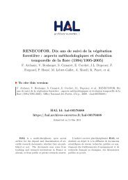
Introductionréponse, l’action et la dynamique des communautés microbiennes sur/face auxchangements environnementaux. Cette sous-discipline fait donc intervenir un large spectrede sciences du vivant comme la biologie moléculaire, l’écologie microbienne, labiogéochimie, etc...2. Les micro-organismes, une source de diversité génétiqueLes micro-organismes sont, par définition, des êtres microscopiques, pour la plupartunicellulaires. La majeure partie de ces organismes appartient aux règnes procaryotesBactéries et Archaea, mais sont aussi représentés chez les eucaryotes comme les Protozoaireset les Fungi (Fig. 1). Les virus, bien que non cellulaires, sont également classés parmi lesmicro-organismes. L’utilisation de la phylogénétique a permis de mettre en évidencel’immense part que prennent les micro-organismes dans la diversité génétique du vivant parrapport aux macro-organismes (Fig. 1; Pace, 1997; Woese, 1998; Finlay, 2002).Figure 1 : Arbre phylogénétiques des êtresvivants. Il est plus simple d’indiquer ici lestaxons ne faisant pas partie des microorganismes: les plantes vertes (encadré vert),certaines algues, et de nombreux métazoaires(encadré violet). Source : Delsuc et al. (2005).Les facteurs responsables d’une telle diversité sont multiples. En effet, ces organismesont un long passé évolutif et un temps de génération relativement court. Les événements demutation ou de recombinaison dans les génomes microbiens sont donc fréquents ets’accumulent depuis longtemps. A cela s’ajoutent les phénomènes de transferts horizontaux(échanges de gènes entre taxons différents) entre procaryotes (Ochman et al., 2000), deprocaryotes à eucaryotes (Katz, 2002) mais aussi entre eucaryotes (Xie et al., 2008).16

IntroductionTous ces remaniements génétiques confèrent aux micro-organismes un tauxd’adaptation élevé. Parallèlement, la planète comporte une multitude de niches écologiques(cf . §III Encadré 2) dont le nombre explose si l’on se place à l’échelle microbienne. Ladiversité des microbes découle donc aussi d’une radiation adaptative dans des nichesécologiques extrêmement diversifiées (revue dans Cohan and Koeppel, 2008), y compris dansles milieux extrêmes, inaccessibles aux organismes supérieurs (revu par Rothschild andMancinelli, 2001).La diversité microbienne est donc vaste. Par exemple, le nombre d’espècesbactériennes du sol a été estimé à plusieurs millions (Curtis et al., 2002), et à près d’unmillion chez les champignons (Bridge and Spooner, 2001; Hawksworth, 2001). De plus, lescellules procaryotes à elles seules représentent près de la moitié de la biomasse de la planète(Whitman et al., 1998). Ainsi, bien qu’ils soient invisibles à l’œil nu, les micro-organismesconstituent une composante essentielle du vivant en termes d’abondance et de diversité.3. Les micro-organismes, acteurs des processus environnementauxLa diversité génétique et la capacité des micro-organismes à coloniser desenvironnements divers, voire extrêmes, indiquent qu’ils possèdent des voies métaboliquesvariées (Pace, 1997). Cette propriété en fait des acteurs clés dans le fonctionnement desécosystèmes (Fig. 2). En effet, les micro-organismes interviennent largement dans les cyclesbiogéochimiques via la dégradation/minéralisation des déchets végétaux ou animaux(Hattenschwiler et al., 2005), et la réallocation des nutriments vers d’autres organismes. De cefait et parce que les populations microbiennes constituent une biomasse importante etrapidement renouvelée, les micro-organismes occupent une place centrale dans les réseauxtrophiques.En agissant sur la qualité et/ou la disponibilité des ressources, les communautésmicrobiennes influencent la diversité et la fitness des espèces environnantes. Cet effet setraduit également à travers le type d’interactions que les membres de ces communautésentretiennent avec les autres organismes le long du continuum parasitisme-mutualisme (vander Heijden et al., 2008). Par exemple, les associations mycorhiziennes peuvent augmenter defaçon plus ou moins directe la productivité des plantes (revue dans Johnson et al., 1997). Al’inverse, une espèce microbienne invasive peut avoir des conséquences dramatiques sur ladiversité en espèce et le fonctionnement d’un écosystème (revue dans Desprez-Loustau et al.,2007). Ces interactions n’ont donc pas seulement un impact sur le fonctionnement des17

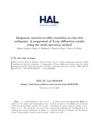
Introductionécosystèmes, elles sont en plus de véritables moteurs de l’évolution par des effets de pressionsélective ou de facilitation.CO 29Figure 2 : Représentation schématique du rôle du compartiment microbien du sol. Les microbes agissent sur ladisponibilité et la réallocation des ressources de façon positive par décomposition, transformation, et transport de lamatière organique et des nutriments vers les plantes (1, 2 et 3), ou négative par séquestration des ressources dans leurbiomasse ou dans la matière organique récalcitrante (4). La diminution de ressources est également due à latransformation de l’azote organique en des composés volatiles ou facilement lessivables (5, 6) qui peut néanmoins êtreacquis via les bactéries fixatrices d’azote atmosphérique (7). Les agents pathogènes induisent quant à eux une diminutionde la productivité des plantes (8). Ces processus sont accompagnés d’efflux de CO 2 via la respiration des microorganismes(9). D’après van der Heijden et al.(2008)18

Introduction4. Les micro-organismes, dimension socio-économiqueLes micro-organismes font partie de notre quotidien de par leur ubiquité et leurrichesse. Responsables de nombreuses maladies aussi bien chez l’homme que chez d’autresespèces, ils constituent un réel problème sanitaire. Certaines périodes sombres de l’histoirerésultent de l’activité pathogène particulièrement virulente de certains micro-organismes.Ainsi, l’invasion du champignon phytopathogène Phytophthora infestans qui frappa l’Irlandeau milieu du XIXème siècle fit chuter la production de la pomme de terre, l’une des causes dela tristement célèbre « grande famine ». Citons également l’épidémie de peste noire, causéepar la bactérie Yersinia pestis, qui décima la moitié de la population Européenne durant leXIVème siècle.Par ce biais les microbes ont mauvaise presse. Pourtant, les relations microbeshommesne sont pas forcément négatives. Certains champignons produisent des fructificationsconsommables, la plus illustre étant la truffe. Les applications industrielles de leurs activitésmétaboliques sont vastes. L’industrie de l’agro-alimentaire en est un exemple frappant : denombreuses souches microbiennes sont utilisées dans des processus de fermentation. Ils sontégalement largement utilisés dans l’industrie pharmaceutique pour la productiond’antibiotiques ou autres médicaments. Capables de dégrader un large panel de moléculescomplexes, leurs enzymes sont utilisées en chimie de synthèse comme catalyseurs deréactions, et comme produits de nettoyage domestiques. Ces aptitudes enzymatiques en fontdes candidats précieux pour la bioremédiation (Dojka et al., 1998; Rothschild and Mancinelli,2001).Les micro-organismes occupent donc une place centrale dans le vivant par leurabondance, leur diversité, et leur implication dans les processusenvironnementaux. L’appréhension du compartiment microbien est donc d’uneimportance capitale pour une meilleure compréhension de ces processus,notamment dans un contexte de diminution de la biodiversité, de pollutionschroniques et, de réchauffement global.19

IntroductionII.Appréhension des communautés microbiennes, les outils1. Les caractéristiques mesurables dans une communauté microbienneL’étude d’une communauté microbienne peut se faire à travers différents indicateurs.Une communauté microbienne se définit par (i) sa biomasse, (ii) sa richesse, sa diversité, sastructure et sa composition en espèces, (iii) ses fonctions dans l’écosystème et la diversité deces fonctions. La biomasse microbienne est responsable de nombreux processusbiogéochimiques et constitue un réel réservoir de matière organique. Elle est sensible auxchangements environnementaux tels que le pH, la couverture végétale ou la fertilité du milieu,ce qui en fait un bon indicateur de la qualité biologique et du fonctionnement desécosystèmes. De même, la composition et la diversité des communautés microbiennes sontfonction des conditions environnementales et peuvent renseigner sur l’état et lefonctionnement de l’écosystème. Enfin, les micro-organismes agissent sur l’environnement àtravers un panel diversifié de voies métaboliques dont la caractérisation peut donner desindications sur les processus environnementaux qui s’y déroulent (Hurst, 2002, cf §III et §IV).Par exemple, des variations de biomasse, de structure et des activités métaboliques descommunautés microbiennes ont été mises en évidence suite à l’augmentation de la quantité demétaux lourds (e.g. Cu, Zn, As ou Cd) (Pennanen et al., 1996; Yao et al., 2003; Lorenz et al.,2006).Toutes ces caractéristiques peuvent être appréhendées via des techniques dites« traditionnelles », basées sur des réactions biochimiques et/ou sur la culture microbiologique,et des techniques moléculaires, plus récentes, basées sur l’ADN ou l’ARN (Table 1). Commenous le verrons plus tard, cette thèse s’articule surtout autour de la structure et de la diversitédes communautés microbiennes. Nous aborderons donc les aspects de biomasse et de fonctionuniquement dans cette partie.2. De l’importance de l’échantillonnageL’échantillonnage joue un rôle crucial dans la caractérisation des communautésmicrobiennes. En effet, (i) les micro-organismes sont extrêmement diversifiés, (ii) il existeune relation aire/espèce chez ces organismes (cf. §III.2, revue dans Green and Bohannan,2006) (iii) leur répartition spatiale varie à l’échelle microscopique. Alors que le point (i) est20

Introductioninhérent à la communauté microbienne considérée et que sa précision relève plutôt desprotocoles expérimentaux utilisés (e.g. profondeur de séquençage, cf §II.4), les points (ii) et(iii) sont déterminés par la stratégie d’échantillonnage.La richesse des micro-organismes dépend effectivement de l’aire d’étude. Enconséquence, le nombre de prélèvements doit être représentatif de la surface de l’écosystèmeétudié. Or, dans le cadre d’une étude comparative de deux sites à priori contrastés, lavariabilité intra-site des communautés microbiennes peut atténuer l’effet inter-site. Cettelimitation peut être contournée par l’analyse d’échantillons composites, c'est-à-dire parmélange des extraits d’ADN issus des réplicas spatiaux d’un même site (Schwarzenbach etal., 2007). En outre, la variabilité spatiale des espèces microbiennes est telle que la quantité desol ou d’eau prélevés a un impact significatif sur les profils moléculaires (Ranjard et al., 2003;Venter et al., 2004). Ainsi, la stratégie d’échantillonnage est déterminante dans lacaractérisation des communautés microbiennes et dans l’estimation de leur diversité.3. Les méthodes dites « classiques »La biomasse microbienne peut être estimée par comptage des cellules microbiennes oupar quantification de la part de carbone que représentent ces cellules (Table 1). D’autresméthodes permettent d’estimer cette biomasse, comme par exemple la spectroscopie procheinfrarouge (NIRS) capable de détecter des composés carbonés typiquement microbiens(Cécillon et al., 2008). Certaines techniques moléculaires donnent également accès à ce typede mesure, comme l’hybridation fluorescente in situ (FISH), qui permet d’observer les microorganismesin situ à l’aide de sondes fluorescentes, ou la PCR quantitative, qui donne accès àla quantité de copies d’un gène donné dont on peut tirer un nombre de cellules (Brouwer etal., 2003).La composition spécifique des communautés microbiennes a longtemps été abordéepar isolement de souches sur des milieux cultures plus ou moins sélectifs (Table 1).L’identification des souches isolées repose alors sur des critères morphologiques (mode degroupement des colonies/hyphes, pigmentation, forme des cellules ou des organes defructification, etc…) et/ou par microscopie, complétés au besoin par des réactionsbiochimiques (réaction de gram, test de l’oxydase, etc…). Cependant, ces méthodes de culturene sont pas forcément représentatives des communautés microbiennes étudiées : il estmaintenant largement reconnu que plus de 99% des microbes n’ont pas encore été cultivés(revu par Amann et al., 1995).21

IntroductionTable 1 : Liste des techniques d’étude des communautés microbiennes, leurs applications, leurs avantages et inconvénients. D’après Tiedje et al, (1999); Hurst (2002); Kirk et al. (2004).MPN : Most Probable Number ; DAPI : Di Aminido Phenyl lndol,; PLFA: PhosphoLipid Fatty Acids; CLPP: Communitiy-Level Physiological Profile; SIGR: Substrate Induced GrowthResponse ; ARDRA: Amplified Ribosomal DNA Restriction Analysis ; ARISA : Automated rRNA Intergenic Spacer Analysis ; T-RFLP : Terminal-Restriction Fragment LengthPolymorphism ; T/DGGE : Temperature/Denaturing Gradient Gel Electrophoresis ; SSCP : Single Strand Conformation Polymorphism.METHODES TRADITIONNELLESMETHODES MOLECULAIRESType de Méthode Exemples Informations Avantages InconvénientsCultureMPN,BiomasseDénombrement surboîteMicroscopieBiochimieApproches basées surla PCR (utilisation demarqueursmoléculaires)Méta-génomique etMéta-transcriptomiqueIsolement, criblagede souchesColoration deGramm, DAPIExtractionfumigationPLFACLPP, SIGRDNA fingerprint:ARDRA, ARISA,T-RFLP, DGGE,TGGE, SSCPClonage/séquençage,pyroséquençageClonage/séquençage,pyroséquençageIdentification morphologique etmétaboliqueIdentification de groupesBiomasseBiomasseBiomasseStructure des communautésBiomassePotentiel métaboliqueStructure des communautés,diversité/richesse (méthodessemi-quantitatives)Caractérisation taxonomiquedes communautés, diversité etrichesse (méthodes semiquantitatives)Caractérisation taxonomique etmétaboliques des communautés,diversité et richesse (méthodesquantitatives)Peu couteux,Rapide si le nombre d’échantillonest faiblePas de biais des non-cultivablesAccès au ratio de biomassechampignons/bactériesPeu coûteux et rapidePas de biais des non-cultivablesSuivi des populations activesRapideScreening d’un grand nombred’échantillonsPas de biais des non-cultivablesReproductibleRapidePas de biais des non-cultivablesReproductiblesRapidePas de biais des non-cultivablesPas de biais de PCRMéthode lourde pour des études à grandeéchelleBiais des non-cultivablesNe reflète pas les conditions in situPas de renseignement sur les populationsactivesMéthode lourde pour des études à grandeéchellePas de renseignement sur les populationsactivesPeu résolutif, surtout pour les champignonsPas de renseignement sur les populationsactivesPas d’identification des populations activesNe reflète pas les conditions in situBiais d’extraction et de PCRChoix d’amorces universellesSaturation de l’information pour descommunautés complexesPas/peu de renseignements taxonomiquesBiais d’extraction et de PCRChoix d’amorces universellesDifficulté du traitement des grands jeux dedonnéesBiais d’extractionDifficulté du traitement des jeux de données22

Introduction4. Les méthodes moléculairesDans les années 60, l’avènement de la biologie moléculaire a permis l’émergence d’unlarge éventail de méthodes basées sur l’ADN qui ont rapidement été appliquées à l’écologiedes communautés chez les micro-organismes. A partir d’un ADN total extrait d’unéchantillon, les communautés microbiennes sont appréhendées soit (i) dans leur ensemble, pardes approches de méta-génomique, soit (ii) de manière dirigée, par amplification par PCR decertaines régions du génome communes à l’ensemble des organismes étudiés (Table 1).Brièvement, un marqueur moléculaire est une région d’ADN variable, permettant ladistinction d’un maximum de taxons, flanquée de régions suffisamment conservées,permettant l’amplification de l’ADN d’un maximum de taxons. Ce sont principalement lesgènes ribosomaux qui sont utilisés pour l’étude des micro-organismes (e.g. gènes de l’ARNr16S chez les procaryotes, ARNr 18S ou 28S et ITS chez les eucaryotes). Toutes ces méthodessont cependant soumises au même biais : l’extraction de l’ADN n’est pas exhaustive(Frostegard et al., 1999; Martin-Laurent et al., 2001).Actuellement, ce sont les méthodes basées sur la PCR, et en particulier les méthodesde type « DNA fingerprint » (empreinte moléculaire) les plus couramment utilisées parcequ’elles permettent le suivi de nombreux échantillons en demeurant accessibles en termes detemps et de coûts. Ces méthodes, reposant sur l’électrophorèse, permettent de séparer desfragments d’ADN selon leur taille (ARISA, ARDRA, T-RFLP) et leur composition en bases(DGGE, TGGE, SSCP). Toutes reposent sur l’amplification par PCR de fragments d’ADN àpartir d’un extrait en raison de (i) une quantité d’ADN inférieure aux seuils de détection et (ii)la complexité de l’extrait d’ADN, constitué d’un ensemble de génomes de nombreuxindividus appartenant à des taxons divers. Les techniques d’empreintes moléculaires sedistinguent aussi par le type de marqueurs moléculaires employé (ARDRA, ARISA) oul’utilisation d’enzymes de restrictions (ARDRA, T-RFLP). Elles donnent cependant accès aumême type d’information, à savoir un profil moléculaire où le nombre et l’intensité des picsreflètent la richesse et l’abondance des phylotypes microbiens (cf. Chapitre I). Ces profilspermettent donc de mettre en évidence des variations de structure et de diversité (Loisel et al.,2006) des communautés induites par des changements environnementaux. Certaines d’entreelles montrent un degré de précision supérieur aux autres (la T-RFLP notamment, Tiedje etal., 1999) mais nécessitent des manipulations supplémentaires, et sont donc plus difficilement23

Introductionapplicables dans le cadre d’études à grande échelle. Cette discussion fait, en partie, l’objet duChapitre I du présent manuscrit.Encadré 1 : Les biais liés au marqueur moléculaire et à la PCR1/ Le choix du marqueur moléculaire estdéterminant dans la finesse et la justesse de l’analyse.En effet, tous les marqueurs ne présentent pas le mêmedegré d’universalité. Il est également possible qu’unmarqueur ne soit pas résolutif pour tous les taxons ciblés.Enfin, les amorces utilisées pour ce marqueur peuventmontrer une certaine spécificité (Anderson et al., 2003).De plus, certains gènes, notamment les gènes ribosomaux,sont répétés dans le génome et le nombre de répétitiondiffère d’un taxon à l’autre (Fig. E1). L’abondance desséquences obtenues n’est donc pas forcémentreprésentative de la communauté réelle.2/L’ADN polymérase provoque des erreurspendant l’amplification par PCR. Les plus mineurs sontles erreurs de « recopiage » qui peuvent influencer lesrésultats (Qiu et al., 2001). Il existe d’autres enzymes plusfidèles de part leur activité exonucléasique (proof-readingpolymerases). L’ADN polymérase ajoute une ou plusieursbases d’adénine en fin de synthèse du brin d’ADN(Brownstein et al., 1996). Ce phénomène modifie la tailleinitiale du fragment. Il est donc critique pour les analysesde type « DNA fingerprint ». Les biais liés à l’ADNpolymérase sont développés dans l’Annexe A.3/L’amplification de mélanges complexes donnelieu à des artéfacts. En effet, il existe des phénomènesd’amplification préférentielle pendant la PCR due auxcaractéristiques des fragments d’ADN, qui ne sont pasprédictibles dans le cadre d’étude des communautés (Polzand Cavanaugh, 1998). De plus, les fragments d’unmélange complexe interagissent entre eux. Cela peutdonner lieu à la formation d’hétéroduplexes, parévénements de recombinaison artificielle, ou de chimères,par saut de l’ADN polymérase d’un fragment à l’autre(Qiu et al., 2001; Thompson et al., 2002). Ces événementssont difficilement évitables.La PCR en émulsion permet de contourner cesartéfacts en amplifiant chaque fragment d’ADN isolémentdans de microgouttelettes, évitant ainsi l’amplificationpréférentielle ou la formation de chimères (Nakano et al.,2003).Figure E1 : Diversité bactérienne de la mer des Sargasses. Chaque couleur correspond à un marqueur moléculaire différent. Notonsla différence d’information que génère chaque marqueur. Par exemple, les gènes ribosomaux surestiment l’abondance desGammaprotéobactéries. Source Venter et al. (2004).24

IntroductionL’utilisation du clonage/séquençage de marqueurs moléculaires permet une analyseplus fine des communautés microbiennes. Brièvement, le séquençage d’un mélange demolécules d’ADN n’est pas possible. Cette limite est contournée par une étape de clonage, quipermet d’isoler chaque fragment d’ADN avant le séquençage. Cette approche est souventemployée de façon complémentaire avec les techniques de cultures pour préciserl’identification taxonomique d’une souche. Cependant, son application principale demeurel’étude de communautés microbiennes complexes car il donne accès non seulement à lacomposition, mais aussi à la richesse et la diversité des communautés microbiennes.Malheureusement, la diversité microbienne est si vaste qu’il est difficile de la caractériserpleinement sans le séquençage d’un grand nombre de clones. En effet, Quince et al. (2008)ont estimé à 4 millions le nombre de séquences de gène de l’ADNr 16S nécessaire pourdécrire 90% d’un métagenome complexe. L’effort de séquençage peut être amélioré parl’utilisation des nouvelles techniques de séquençage massif, comme le pyroséquençage(Margulies et al., 2005). Il est cependant nécessaire de garder en tête que les techniquesbasées sur l’amplification par PCR sont soumises à des biais (Encadré 1), limitationsauxquelles les approches méta-génomiques ne sont pas soumises puisqu’elles consistent àséquencer de façon non dirigée l’ensemble des génomes contenus dans un échantillon.L’émergence des nouvelles technologies de séquençage est une étape majeure dans lacaractérisation des communautés microbiennes, puisqu’elle permet d’augmenter de façonsignificative l’effort de séquençage. Cependant ces techniques génèrent parallèlement uneautre limite ; celle de l’analyse de jeux de données contenant des centaines de milliers deséquences (cf. chapitre 3).Les méthodes d’analyse des communautés microbiennes sont donc variées, maisaucune n’est exhaustive. Chacune d’entre elles présente ses limites qui serépercutent de manière différente sur les résultats obtenus. Ce n’est donc que parla définition d’une bonne stratégie d’échantillonnage et par la conjugaison detechniques d’approches complémentaires adaptées à la question biologique quel’appréhension des communautés microbiennes peut être optimisée.25

IntroductionIII. Appréhension des communautés microbiennes, les concepts1. Comment définir une espèce microbienne ?La compréhension du compartiment microbien et de son rôle dans l’environnementnécessite l’identification des individus qui le composent. Cette identification repose sur laclassification de ces individus en groupes partageant un certains nombre de caractéristiques.Ces caractéristiques peuvent être génétiques, fonctionnelles, ou systématiques (i.e.taxonomiques). Or ces critères de classification possèdent des niveaux d’organisationhiérarchiques. Par exemple : doit-on grouper ensemble les individus partageant 70 ou 90% deleur génome ? Doit-on classer les individus selon leur capacité à dégrader certains composésou selon le type de voies métaboliques employées dans la dégradation de ces composés ?Puisqu’une unité universelle de classification des organismes relève de l’utopie, leregroupement des individus selon certains critères nécessite la fixation de seuils. Bien que lataxonomie présente également une organisation hiérarchique, les seuils définis par celle-cisont fixes, utilisés depuis des siècles, et paraissent donc plus intuitifs. Ainsi, la plupart desétudes en écologie des communautés sont basées sur une unité, l’espèce.Chez les macro-organismes, une espèce se définit principalement par l’isolementreproductif des individus qui la composent. Au sein d’une population, cette spéciation peutêtre due soit à un isolement physique qui mène à la spéciation par dérive génétique(spéciation allopatrique), soit à des événements de recombinaison génétique limitant lecroisement de certains individus (spéciation sympatrique). Or, cette notion d’espèce estbeaucoup plus complexe chez les micro-organismes (Encadré 2). En effet, ils présentent laplupart du temps une reproduction clonale rendant difficile l’observation d’un isolementgénétique franc (Fig. 3a ; Taylor et al., 2000; Acinas et al., 2004). La complexité de cettenotion est accentuée par les phénomènes de transfert horizontaux, courant chez les microorganismes(Ochman et al., 2000, cf. §I.2), qui tendent à générer des génomes « enmosaïque » (Tyson et al., 2004). Enfin, les micro-organismes possèdent une importanteplasticité phénotypique au niveau « intra-spécifique », que ce soit en termes de morphologie(Rainey and Travisano, 1998, Fig. 3b) ou d’activité enzymatique (revue dans Deitsch et al.,1997; Buee et al., 2007) rendant impossible toute classification sur critères morphologiques etéco-physiologiques. Ainsi, la découverte d’espèces cryptiques au sein d’espèces microbiennes26

Introductionprédéfinies a amené la communauté scientifique à revisiter le concept d’espèce chez lesmicro-organismes (Encadré 2)(a)(b)Figure 3 : Des difficultés dans la classification des micro-organismes. (a) Arbre Bayesien d’espèces bactériennes(une couleur par espèce) du genre Nesseria. Alors que les espèces rouges, bleues et vertes paraissent clairementdéfinies, les autres ne présentent pas d’isolement génétique franc. Source : (Achtman and Wagner, 2008). (b) diversitémorphologique des colonies de Pseudomonas fluorescens SBW25 en réponse à des variations environnementales.Source : Rainey and Travisano (1998).Dans ce contexte, il est ardu d’établir des groupes d’individus distincts dans unecommunauté microbienne. De plus, les différents concepts de l’espèce microbienne (Encadré2) sont difficilement applicables à l’échelle de la communauté parce qu’ils nécessitentl’acquisition et la comparaison de génomes entiers (cf. §II.4). Malgré ces limitations, lecomportement des communautés microbienne et de leur diversité sont abondammentdocumentés (e.g. Venter et al., 2004; O’Brien et al., 2005; Fierer and Jackson, 2006; Fierer etal., 2007b). Ces études sont basées sur la systématique moléculaire soit (i) par une approchemultilocus (screening et phylogénie de plusieurs gènes), qui reste difficilement applicable àl’échelle de la communauté, soit (ii) par criblage et/ou phylogénie des gènes ribosomaux,consistant à étudier l’identité, la richesse, la diversité et/ou l’affiliation phylogénétique desunités taxonomiques opérationnelles (OTUs), composées par des rybotypes (séquencesribosomales) similaires. Bien que cette approche ne présente pas de justification théorique(Encadré 2) et soit limitée par les techniques expérimentales (cf. § II.4), elle a néanmoinspermis de s’affranchir des limites causées par le manque de consensus autour du conceptd’espèce microbienne, et par notre incapacité actuelle à isoler en culture la majorité de cesorganismes (revu par Amann et al., 1995). Cette approche a en outre donné accès à certains27

Introductionphénomènes dans le comportement des communautés microbiennes que nous évoquerons plustard.Encadré 2 : les différents concepts d’espèce microbienneLes critères de classification des micro-organismes enespèces sont maintenant divers. Certains considèrentqu’une espèce doit être monophylétique et présenter unecohésion génomique et phénotypique. D’autre pensentqu’elle se définit en fonction du taux de transfertshorizontaux, plus élevé au sein d’un groupe qu’entregroupes Certains considèrent enfin que le conceptd’espèce n’est pas applicable aux microbes (revu parAchtman and Wagner, 2008).Malgré ce manque de consensus, il apparaît que lesmicrobes peuvent être classifiés par le concept de pangénome.Celui-ci comprend un pool de gènes commun àtous les individus, le « core-genome », et un répertoire degènes peu/pas partagés, le « dispensable genome »,responsable de la plasticité écophysiologique du groupeet lui conférant son pouvoir adaptatif (Medini et al., 2008,Fig. E2).La notion de pan-génome englobe celle d’écotype, quiréfère à un groupe d’individus écologiquement similaires àun autre mais présentant une certaine cohésion génétiquecausée par la sélection et/ou la dérive génétique (revu parCohan and Perry, 2007, Fig. E2).La définition d’espèce chez les micro-eucaryotessemble suivre le même schéma. Cependant, les conceptsd’espèce chez ces organismes sont plutôt d’ordreopérationnel (i.e. méthodologiques, Taylor et al., 2000)que théorique (mais voir Kohn, 2005; Giraud et al., 2008)Le concept d’espèce microbienne apparait donccomme une sorte de continuum où certains individusforment des groupes distincts et d’autres des groupesmoins définis (revue dans Achtman and Wagner, 2008),Fig. 3a). Les critères de classification des microbesdépendent donc de la question biologique posée.Figure E2 : Représentation schématique des principaux concepts d’espèce microbienne. D’après Medini et al. (2008)Communauté (Méta-génome)Pan-génomeEcotypeGénomeEnvironnement2. Les patrons de distribution spatiale des micro-organismesNous avons précédemment vu que les micro-organismes ont colonisé la quasi-totalitéde la planète. Mais malgré cette ubiquité, les « espèces » microbiennes et leur assemblagesuivent-ils des patrons de distribution similaires à ceux des macro-organismes (Encadré 3) ?28

IntroductionS’il on en croit le vieil adage de la microbiologie défini par Baas-Becking et inspiré destravaux de Beijerinck, « everything is everywhere, but, the environment selects » (Quispel,1998). Ceci implique que les micro-organismes ont une biomasse et une capacité dedispersion telles que leur présence est possible dans n’importe quel environnement, mais queles contraintes environnementales locales ne favorisent que certaines espèces. Cette doctrineest toujours débattue à ce jour, certains supportant le cosmopolitisme des micro-organismes(Finlay, 2002; Fenchel and Finlay, 2003), et d’autres soutenant le contraire (e.g. Cho andTiedje, 2000; Whitaker et al., 2003; Taylor et al., 2006; Halling et al., 2008).Encadré 3 : Quelques notions d’écologie des communautésLa distribution des organismes découle de différentsfacteurs. Premièrement, les facteurs écologiques (e.g.température, disponibilité en eau, interactions biotiques,etc…) agissent comme des filtres sur les espèces (Belyeaand Lancaster, 1999; Lavorel and Garnier, 2002, Fig. E3).En effet, les conditions environnementales définissent desniches écologiques. Ces niches présentent différentsniveaux d’organisation, e.g. la caractéristique « fertilité »englobe les caractéristiques de quantités de nitrates et dephosphore. A l’intérieur de ces niches, deux espèces nepeuvent coexister durablement que si leurs besoinsdiffèrent à un niveau d’organisation inférieur de la niche(principe d’exclusion compétitive). L’assemblage desespèces sur un site donné résulte donc en partie del’assemblage des niches de ce site.Deuxièmement, les demandes et les réponses d’uneespèce a vis-à-vis d’une niche la rendent plus ou moinsapte à s’adapter et à se maintenir dans un milieu. Cesfacteurs biologiques, inhérents à l’espèce, sont de mêmeordre chez les espèces occupant des niches similaires,même si celles-ci sont géographiquement distantes. Lestaux de dispersion et de spéciation de l’espèce, quidéterminent sa capacité à coloniser le milieu, sontégalement des facteurs biologiques.Enfin, les interactions biotique/abiotique sontdynamiques (Fig. E3). La distribution des espècesdépend donc aussi de facteurs historiques, qui renvoientà la succession de peuplements et de conditionsenvironnementales qui ont contribué à l’état actuel dusite considéré (Bardgett, 2005; Hughes Martiny et al.,2006).Figure E3 : Représentation schématique du fonctionnement d’un système. Il existe trois grandes composantes en biogéographie :la structure biologique considérée, l’espace, et le temps (soulignés), chacune présentant différents niveaux d’organisation. Cescomposantes interagissent, et leurs différents niveaux d’organisation ont une répercussion les uns sur les autresRégionalPaysageLocalSuccessionSaison/AnnéeHeure/JourComposante spatialeCompartiment abiotiqueComposantehistoriqueCompartiment biotiqueMéta-communautéCommunautéPopulationDistributiongéographique desespècesAssemblage descommunautés29

IntroductionAvant d’aller plus loin dans ce débat, il est nécessaire de redéfinir certainescaractéristiques propres aux micro-organismes. Chez les macro-organismes, une communautése structure selon un schéma bien établi. Elle est composée de quelques espèces largementdominantes, accompagnées par des subordonnées. On y trouve aussi des espèces dites de« transition », souvent insubordonnées aux espèces dominantes, plus rares, et beaucoup plusdiverses (Grime, 1998) Les communautés microbiennes suivent des règles similaires (Hugheset al., 2001; Zhou et al., 2002; Tedersoo et al., 2008) mais montrent une diversité d’espècesrares bien supérieure à celle des macro-organismes, désignée comme la « biosphère rare »(Sogin et al., 2006). Tout comme chez les végétaux, la diversité de ces espèces rares pourraitêtre impliquée dans la résilience des écosystèmes suite à différents degrés de perturbations(Grime, 1998; Sogin et al., 2006). De la même manière, la relation aire-espèce existant chezles macro-organismes a également été rapportée chez les micro-organismes. Cette relationapparaît généralement plus faible en raison de leur diversité. Cependant, cette observation estsoumise à caution étant donné (i) qu’aucune technique d’approche des communautés n’estexhaustive (cf. §II), (ii) que cette relation varie avec la résolution taxonomique, et (iii) que lesétudes sur le sujet n’utilisent pas des stratégies d’échantillonnage et des techniquescomparables (revue dans Green and Bohannan, 2006).Les microbes montrent aussi certaines caractéristiques fondamentales impliquées dansleurs patrons de distribution. La plupart possèdent un taux de dispersion élevé de part leurpetite taille ou celle de leurs spores. Cette dispersion se fait de manière passive, vial’atmosphère et l’eau, mais peut aussi être inféodée à la migration d’autres organismes. Deplus, les micro-organismes ont un taux de spéciation élevé en raison (i) d’une action de lasélection rapide due à un temps de génération court, et (ii) de l’acquisition de traitsécologiques avantageux par transferts horizontaux de gènes provenant des micro-organismesautochtones (cf §I.2 et §III.1). En raison de ces caractéristiques, il est possible que lesmicrobes connaissent un taux d’extinction plus faible, sachant de plus que certains d’entreeux sont capables de sporuler ou d'entrer dans des phases de vie leur permettant de résisteraux stress environnementaux (Horner-Devine et al., 2004; Kohn, 2005; Ramette and Tiedje,2007).Il semble que l’assemblage des communautés microbiennes soit soumis à des règleséquivalentes à celles influençant les macro-organismes (Encadré 3). Notre incapacité àcultiver la majorité des micro-organismes indique déjà leur inégalité face aux conditionsenvironnementales. De nombreuses études abondent dans ce sens et ont pu mettre en évidence30

Introductionl’impact du pH, de la disponibilité des ressources ou de l’utilisation des terres sur la structureet la diversité des communautés microbiennes (e.g. Zhou et al., 2002; Green et al., 2004;Fierer and Jackson, 2006; Kasel et al., 2008; Lauber et al., 2008; cf §IV), donnant à penserque ces communautés suivent des patrons de distributions non-aléatoires, en fonction desconditions environnementales.De plus, d’autres études ont également révélé une certaine dissimilarité descommunautés microbiennes (Green et al., 2004; Fulthorpe et al., 2008), voire un certain degréd’endémisme des espèces, avec l’augmentation de la distance géographique (Cho and Tiedje,2000; Taylor et al., 2006; Halling et al., 2008). Ces études montrent que l’isolementgéographique, et par conséquent historique, est un moteur de spéciation qui influence lacomposition des communautés microbiennes (Fig. 4, revue dans Hughes Martiny et al., 2006),rejoignant par ce fait les facteurs régissant la distribution des macro-organismes (Encadré 3).En somme, les communautés microbiennes tendent à se ressembler si leur environnement seressemble, quelle que soit l’échelle d’observation (i.e. province ou ensemble de provinces),mais tendent à se différencier avec l’éloignement géographique (Fig. 4, revu Hughes Martinyet al., 2006). Cependant, la majorité des études portant sur l’endémisme des micro-organismesen fonction de la distance géographique ont été menées dans des écosystèmes possédant descaractéristiques radicalement différentes (e.g. couvert végétal, type de sol, etc..). Dans cecontexte, il est difficile de dissocier la part des facteurs écologiques de celle de l’éloignementgéographique dans la différenciation des communautés ou dans la spéciation. Par exemple,(Fierer et al., 2007a) ont observé un effet de l’environnement supérieur à celui de la distancegéographique à l’échelle du bassin versant.Figure 4 : Effets supposés des composantesécologiques et historiques sur les communautésmicrobiennes. Un habitat définit un type de conditionsenvironnementales (conditions abiotiques et couvertvégétal). Une province représente une airegéographique dont le passé évolutif est homogène (e.g.un continent). Une province inclut donc plusieurshabitats. Source Hughes Martiny et al. (2006).31

IntroductionEn considérant toutes ces caractéristiques propres aux micro-organismes, une« espèce » microbienne est susceptible d’avoir une aire de répartition beaucoup plus étenduequ’une macro-espèce via un taux de dispersion élevé. Cette étendue apparaît néanmoinslimitée par le fort taux de spéciation de ces organismes couplé à la distribution des nichesécologiques, ainsi que par la dépendance de certains de ces organismes à un hôte. Cependant,un taux d’extinction faible autorise la présence d’espèces inadaptées à l’environnement par lesphénomènes que nous avons précédemment cité. Cette propriété corrèle avec la diversité vastede la « rare biosphère » observée par (Sogin et al., 2006) et composée de nombreuses espècesde très faible abondance. Cette biosphère apparaît comme un accumulateur, indépendant dusuccès de l’espèce, de spores/souches se trouvant ou s’étant trouvées dans le milieu, rappelantainsi les « banques de graines » observées chez les végétaux. Or, une telle diversité d’espècesrares est difficilement accessible de manière exhaustive avec les techniques utilisées enmicrobiologie environnementale (cf §II), et la part des populations effectivement actives dansces communautés l’est encore plus. La composition spécifique réelle de ces communautésreste donc inaccessible.Ainsi, le débat d’une biogéographie des micro-organismes semble donc davantage undébat sémantique plutôt que conceptuel. La doctrine de Baas-Becking possède un sens large,aux interprétations variées (de Wit and Bouvier, 2006). Les acteurs de ce débat ne secontredisent pas quant à l’impact indéniable des facteurs environnementaux sur la structuredes communautés microbiennes, mais n’utilisent ni les mêmes critères de définition del’espèce, ni la même profondeur d’échantillonnage, ce qui conduit forcément à unedivergence d’opinion face à la question de biogéographie microbienne.3. Quid de la dynamique des communautés microbiennes ?L’assemblage des communautés varie non seulement dans l’espace (Encadré 3), maisaussi dans le temps. En effet, les facteurs biotiques et abiotiques responsables de la présenced’une espèce sont eux-mêmes soumis à une dynamique qui s’opère sur une hiérarchie de pasde temps. Ainsi, les processus de colonisation et d’extinction d’espèces sur un site donné suiteà une modification de l’habitat sont définis en écologie comme des successions. Cettesuccession suit une trajectoire dépendant de la nature de la perturbation de l’habitat, desespèces amenées à coloniser le milieu et/ou déjà présentes dans ce milieu sous forme latente,ainsi que des conditions climatiques. Ces processus s’opèrent de manière continue, sur despas de temps de l’ordre de l’année ou de la décennie chez les macro-organismes.32

IntroductionA l’échelle microbienne, l’impact des changements environnementaux surl’assemblage des communautés peuvent s’opérer sur des pas de temps beaucoup plus courts(journée, saisons). En effet, à un niveau local, la disponibilité des ressources peut varier à trèscourt terme et ainsi rapidement influencer la structure des communautés microbiennes(Pinhassi et al., 1999; Bardgett et al., 2005b; Schmidt et al., 2007). A l’échelle de la semaineou du mois, des stress tels que des événements de gel-dégel, de sécheresse/humidification, oude pollution peuvent affecter la communauté (Bardgett, 2005). Ces changements s’opèrentégalement en fonction des saisons, avec le développement de la végétation et les fluctuationsclimatiques (Murray et al., 1998; Bardgett et al., 2005b; Nemergut et al., 2005; Schmidt et al.,2007). Enfin, l’évolution des communautés microbiennes varie sur des pas de temps beaucoupplus long, en parallèle à la succession des communautés végétales (Ohtonen et al., 1999;Bardgett et al., 2005b).(a)Population density (mg FW/L)Phytoplankton(b)Clone frequencyTime (days)BacteriaFigure 5 : Dynamique des communautés microbiennes dans des environnements stables. (a) Dynamique d’unecommunauté de phytoplancton d’une dizaine d’espèces (vert : flagellés verts, bleu : pico-phytoplancton procaryote,rouge : les diatoméées du genre Melosira. Source : Scheffer et al. (2003). (b)/ Dynamique de la communautébactérienne d’un réacteur méthanogénique (chaque couleur représente un OTU, le motif représente des séquencesuniques). Source : Fernandez et al. (1999)Il est également possible d’observer des fluctuations des communautés microbiennesindépendamment des conditions environnementales (hors disponibilité des ressources). Lesinteractions entre les protagonistes de la communauté sont de natures diverses et s’articulentle long du continuum parasitisme-mutualisme (cf. §IV.4). Enfin, ces communautés formentdes chaînes trophiques, et transforment continuellement les ressources du milieu de manièrequalitative et quantitative. Ainsi, plusieurs auteurs ont mis en évidence l’instabilité despopulations microbiennes dans des conditions pourtant stables (Fernandez et al., 1999;Scheffer et al., 2003; Becks et al., 2005; Fig. 5). Ces fluctuations ont été jugées d’ordre33

Introductionchaotique (Becks et al., 2005), mais ne semblent pas modifier le fonctionnement del’écosystème (Fernandez et al., 1999).La dynamique des communautés microbiennes semble donc liée à des mécanismescomplexes, encore difficiles à cerner en raison des facteurs indénombrables impliqués dans ceprocessus. Néanmoins, ce comportement apparemment chaotique peut être expliqué parl’opportunisme écologique des espèces de la communauté en réponse à des changementsinfimes des conditions environnementales (Rainey et al., 2005).En résumé, il existe un réel manque de cadre conceptuel dans l’appréhension ducompartiment microbien. Les concepts tirés des patrons de diversité, derépartition et de dynamique des macro-organismes ne peuvent être appliquésdirectement aux micro-organismes en raison de leur petite taille, de leur grandediversité et d’une dynamique des communautés rapides. Finalement, la questionn’est pas de savoir si les micro-organsimes suivent les mêmes lois que les macroorganismes,mais plutôt de savoir quelle est l’échelle à laquelle les patronsmicrobiens se rapprochent au mieux de ceux des macro-organismes (Green andBohannan, 2006).34

IntroductionIV. Les communautés microbiennes du sol, une étape de plus versla complexité1. De l’importance des solsEn raison d’une diversité, d’une abondance et d’une dispersion élevées, les microorganismesont colonisé la quasi-totalité de la surface planétaire. De nombreuses études lesdécrivent dans des écosystèmes marins (e.g. (Moon-van der Staay et al., 2001; Thorseth et al.,2001; Venter et al., 2004)), des environnements extrêmes (e.g. milieux acides, hyper salins,anoxiques, secs, contaminés, etc…, revu par Rothschild and Mancinelli, 2001), desenvironnements biologiques (e.g. tube digestif, racines, etc; Backhed et al., 2005), maissurtout dans les sols (revu par Tiedje et al., 1999; Torsvik and Ovreas, 2002; Anderson andCairney, 2004; Foissner, 2006). Par exemple, un gramme de sol provenant d’un champ peutcontenir 10 9 bactéries, 10 5 protozoaires et 1 km de mycélium (Young and Ritz, 2005).Le sol se définit comme étant la couche superficielle meuble de l’écorce terrestre. Ilest issu d’interactions entre une matrice physico-chimique de composition extrêmementvariable et une grande diversité d’organismes. Il n’est donc pas qu’un simple support des êtresvivants ; il constitue aussi un important stock de matière organique et minérale, abritant unegrande diversité d’êtres vivants (Fig. 6). En conséquence, il s’y déroule de nombreuxprocessus biogéochimiques dont les acteurs sont variés. Le sol est donc un véritablecarrefour multifonctionnel (Gobat et al., 2003) et occupe une place centrale dans lefonctionnement des écosystèmes terrestres. Représentant près d’un tiers de la surface de laplanète, les services rendus par le sol s’appliquent non seulement aux milieux naturels, maisaussi aux systèmes anthropiques en regard de l’agriculture ou la gestion des déchets(Costanza et al., 1997).Le sol est un compartiment extrêmement hétérogène. Ses caractéristiques varient àpetite échelle, selon la répartition des pores, des agrégats, des racines, des nutriments et del’eau (Young and Crawford, 2004, Fig. 6), mais aussi à plus grande échelle, en fonction de laroche mère, du climat et de la couverture végétale (Hooper et al., 2000; Ettema and Wardle,2002). De la même manière, les caractéristiques du sol peuvent changer dans l’heure ou dansla journée, d’une saison à l’autre, et évoluent au cours des successions (Bardgett et al.,2005b). C’est donc un compartiment diversifié et dynamique ; en 4 dimensions : surface,35

Introductionprofondeur et temps. De part sa complexité, il constitue une réelle « boîte noire » des sciencesenvironnementales.(a)(c)(e)(b)(d)(f)Figure 6 : Les organismes du sol dans leur habitat. Visualisation en coupe mince d’un sol. a/ Mycelium deRhizoctonia solani. b/ Un mycelium non-identifié et des sporanges répartis dans un pore. c/ Une amibe se faufile dans unpore étroit. d/ Amibes à thèque s’accumulant près d’un pore. La flèche désigne une colonie bactérienne. e/ Nématodeprobablement distordu par la forme du pore qu’il occupe. f/ Coupe tangentielle d’une Enchytraeidae (vers) adjacentes àune racine en décomposition (à gauche). Cette image montre la présence de sol dans le lumen du tube digestif du vers(portion supérieure), et une distorsion du corps de l’animal par les limites du pore. Ces images proviennent d’un mêmesol. Source : Young and Ritz (2005).Le compartiment sol a longtemps été étudié séparément du compartiment aérien.Cependant, un nombre croissant d’études a permis de mettre en évidence l’étroite relationqu’entretiennent ces deux systèmes (Hooper et al., 2000; Bardgett et al., 2005a; van derHeijden et al., 2008). Comme nous l’avons précédemment évoqué, les microbes du solinfluencent le fonctionnement des écosystèmes ainsi que la fitness et la diversité des espècesenvironnantes (cf §I.3). Mais qu’en est-il des facteurs influençant le compartiment microbiendes sols ?36

Introduction2. Des facteurs abiotiques régulant les communautés microbiennesL’habitat des micro-organismes du sol est constitué de pores variant dans l’espace(Fig. 6) et le temps, lui conférant une extrême hétérogénéité. La taille et la répartition de cespores sont essentielles dans la conduction de l’eau et des nutriments, ainsi que dans lacommunication entre les différentes populations microbiennes (Torsvik and Ovreas, 2002;Young and Ritz, 2005; Standing and Killham, 2007). Ce sont des habitats généralementpauvres et peu favorables au développement de populations microbiennes à forte densité et àactivité intense. C’est surtout dans la rhizosphère que les communautés microbiennes semontrent les plus denses et les plus actives (cf §IV.2).Les mouvements d’eau sont primordiaux pour le maintien de la vie dans le sol. Ilspermettent effectivement la diffusion des ions, des nutriments et des gaz dissous, etmaintiennent une température favorable aux organismes autochtones. La mobilité de laplupart des micro-organismes étant inféodée à l’eau, ces mouvements d’eau sont égalementresponsables de la dispersion et la connectivité des populations microbiennes. Ces connexionspeuvent avoir des effets négatifs, comme une augmentation de la prédation, mais aussipositifs, en augmentant les flux de gènes et les échanges trophiques. Enfin, l’eau influencefortement le pH du sol (Standing and Killham, 2007). Ce pH n’est pas seulement influencépar l’eau, mais aussi par la nature de la roche mère, la qualité de la matière organique, et parl’activité microbienne. Or, le pH a un effet dramatique sur les communautés microbiennes. Eneffet, basé sur la technique de PLFA (Baath and Anderson, 2003) ont montré une corrélationpositive entre le pH du sol et le ratio champignons/bactéries dans des hêtraies chênaieshêtraies.Basé sur la même technique, l’étude de (Hogberg et al., 2007) le long d’un gradientde pH a mis en évidence une corrélation entre le pH et la biomasse microbienne, positive chezles bactéries, et négative chez les champignons. Les fluctuations de pH induisent égalementdes variations de composition, de structure et de diversité des communautés microbiennes,auxquelles les bactéries apparaissent particulièrement sensibles (Baath and Anderson, 2003;Fierer and Jackson, 2006; Lauber et al., 2008).La température des sols est également un facteur déterminant dans la distribution etl’activité des micro-organismes, en particulier pour les processus d’ammonification et denitrification. Cette température affecte non seulement la physiologie des micro-organismes,mais influencent aussi les mouvements d’eau et la diffusion des gaz et des nutriments(Standing and Killham, 2007). Les micro-organismes ne montrent pas tous la même tolérance37

Introductionface à la température, et on distingue ainsi les psychrophiles supportant des températuresallant de -5 à 20 °C ; des mésophiles, qui tolèrent des températures de 15 à 45 °C ; et desthermophiles supportant des températures de 65 à 95°C (Rothschild and Mancinelli, 2001;Standing and Killham, 2007).D’autres facteurs abiotiques influencent les communautés microbiennes. L’énergielumineuse a, entre autres, un effet principalement indirect, via la stimulation de la germinationet de la croissance de la végétation. Elle peut cependant avoir une action directe sur les microorganismesphototrophes (Standing and Killham, 2007). Enfin, la quantité et la qualité de lamatière organique du sol est la source principale d’énergie des communautés microbiennes.La qualité de cette matière organique est très variable, allant de composés facilementdégradables (comme les monomères glucidiques solubles) à d’autres récalcitrants (polymèreinsolubles comme la lignine). Les caractéristiques de la matière organique peuvent en outreaffecter les propriétés physico-chimiques du sol, comme le pH. Cette matière organique estgénéralement perçue comme une matière morte (e.g. litière, fèces, etc…), bien que labiomasse microbienne constitue une part importante de cette matière organique. Provenantd’êtres vivants, ses effets sur les communautés microbiennes seront abordés ci-dessous.3. Des facteurs biotiques régulant les communautés microbiennes ; lecompartiment aérienLe sol est perpétuellement enrichi par la matière organique provenant des organismesdu compartiment aérien, dont les plantes sont les principaux contributeurs (cf §I.3). Cesentrées de ressources sont variables et leur qualité et quantité sont intrinsèquement liées à lanature de la végétation sus-jacente. En effet, les végétaux peuvent être classés selon leurstraits fonctionnels, i.e. leurs caractéristiques morphologiques, biochimiques et reproductives(e.g. taux de croissance, absorption des nutriments, dégradabilité...). Ces traits co-varient avecles conditions environnementales par effet de rétroaction (i.e. réponse et effet, revue dans[Eviner and Chapin, 2003]). A l’échelle de la communauté, le type de réponses/effets face auxcontraintes environnementales est principalement porté par les espèces dominantes quiconstituent une part importante de la biomasse (Grime, 1998). Ainsi, les contraintesenvironnementales et les groupes fonctionnels dominants déterminent le fonctionnement desécosystèmes, notamment à travers la production primaire et la décomposition (Grime, 1998;Lavorel and Garnier, 2002).38

IntroductionCes traits fonctionnels influencent donc la qualité et la quantité de litière (Fig. 7a). Or,la qualité des ressources du sol influence de manière significative les communautésmicrobiennes (Zhou et al., 2002; Wardle et al., 2004; Chapman et al., 2006; Lauber et al.,2008). Ainsi, plusieurs études ont mis en évidence l’effet de l’utilisation des terres ou ducouvert végétal sur les communautés microbiennes (Fierer and Jackson, 2006; Yao et al.,2006; Zak and Kling, 2006; Kasel et al., 2008; Lauber et al., 2008). De plus, l’augmentationde la récalcitrance de la matière organique provoque une diminution de la biomassemicrobienne, et pourrait parallèlement résulter en une augmentation de la diversitéfonctionnelle de ces communautés (Hopkins and Gregorich, 2005). Cependant, l’impact de laqualité de la litière, et indirectement celui de la diversité fonctionnelle des communautésvégétales, sur la diversité et le recrutement des espèces microbiennes restent encore malcaractérisés.La productivité du milieu, ou l’apport des ressources, régulent la diversité des macroorganismes.Cette relation est unimodale, et le maximum de diversité est atteint à des niveauxintermédiaires de productivité. Il semble que cette relation productivité-diversité soit similairechez les micro-organismes tant bien en milieu aquatique (Horner-Devine et al., 2003), qu’enmilieu terrestre (Bardgett et al., 2005a; Waldrop et al., 2006, Fig. 7b).La composition de la végétation peut aussi influencer les communautés microbiennes,particulièrement celles associées aux racines soit par leur capacité à sécréter des métabolitessecondaires antimicrobiens, soit par leur vulnérabilité face aux pathogènes, soit enfin par lesassociations qu’elles établissent avec les micro-organismes, comme les mycorhizes.Cependant, l’association entre une espèce hôte et une espèce microbienne est rarementobligatoire (Allen et al., 1995; Gardes and Dahlberg, 1996) et il est difficile de statuer surl’existence d’une relation entre la diversité en espèce des communautés végétales, et celle desmicro-organismes du sol. En effet, bien qu’il semble exister une relation entre la diversité descommunautés végétales et celle des communautés microbiennes (Wardle et al., 2004), cetterelation dépend du contexte de l’étude. Par exemple, Waldrop et al. (2006) (Fig. 7b), n’ontpas observé d’effet direct de la diversité des communautés végétales sur la diversité deschampignons du sol. De la même manière, une seule espèce d’arbre peut favoriser la diversitémicrobienne en rendant le milieu beaucoup plus hétérogène en termes de structure et deressources qu’une pelouse diversifiée (revue dans Hooper et al., 2000).39

Introduction(a)(b)+-+-+-Figure 7 : La nature des communautés végétales influence la disponibilité des ressources et le fonctionnementdes sols. (a) les espèces à croissance rapide ont une litière plus facilement dégradable, favorisant la biomassebactérienne. Ces espèces sont également soumises à d’avantage d’herbivorie. Ces systèmes sont donc fertiles et lesprocessus de recyclage de la matière organique sont rapides. A contrario, les espèces à croissances lentes ont unelitière récalcitrante, moins accessible aux bactéries. La biomasse fongique est donc plus elevée mais les processus derecyclage de la matière organique restent faibles. D’après Wardle et al. (2004). (b) la diversité des communautésvégétales ne semble pas affecter la diversité fongique, mais celle-ci apparaît clairement dépendante de la productivitédu milieu (ici assimilée comme étant la biomasse microbienne). D’après Waldrop et al. (2006).La végétation influence aussi ces communautés à une échelle locale, dans larhizosphère. En effet, les racines des plantes contribuent à la structuration du sol, serenouvèlent en permanence, et produisent des exsudats (e.g. carbohydrates, acides organiques,acides aminés) dont la qualité et la production sont variables dans le temps et selon la plante,(Bardgett et al., 2005b; Bais et al., 2006; Standing and Killham, 2007). En effet, le stade dedéveloppement de la plante et la rhizodéposition ont un impact significatif sur la structure descommunautés microbiennes de la rhizosphère de Medicago truncatula, Chrysanthemum etLolium multiflorum (Duineveld et al., 2001; Butler et al., 2003; Mougel et al., 2006).40

IntroductionEnfin, les ressources du sol sont utilisées par des acteurs divers. Parmi ces ressources,l’azote est le plus abondamment documenté en raison de son importance dans la croissancedes végétaux. Or, il existe une compétition entre les plantes et le compartiment sous-terrainpour cette ressource, comme l’ont montré entre autres les études de (Lipson et al., 1999) et(Jonasson et al., 1999) qui peuvent réduire la productivité des plantes (van der Heijden et al.,2008). Les relations entre les communautés végétales et les micro-organismes du sol sontabordées dans les Chapitres 2 et 3 du présent manuscrit.4. Des facteurs biotiques régulant les communautés microbiennes ; lecompartiment sous-terrainLes communautés microbiennes du sol sont également fortement influencées par lesinteractions qu’entretiennent les espèces du compartiment souterrain. Ces interactions ont lieuà une échelle bien inférieure à celle des animaux ou des végétaux. En effet, la structure du solpartitionne les communautés microbiennes dans des micro-niches. Ces « îlots » depopulations microbiennes peuvent être connectés par des mouvements d’eau, par la croissancede racines des plantes ou celle du mycélium fongique, et par la mobilité de la faune du sol. Lafragmentation des communautés microbiennes du sol et leur degré de connectivité sontdéterminantes dans leurs interactions physiques, biochimiques, et trophiques (Encadré 4,Van Elsas et al., 2007).Les interactions biotiques sont habituellement classées le long d’un continuum entreles bénéfices et les pertes résultant de l’interaction (Fig. 8). Précisons ici que la nature de cesinteractions n’est pas toujours fixe, et qu’elle peut se déplacer le long du continuumparasitisme/mutualisme au cours de l’existence des protagonistes de l‘interaction (Johnson etal., 1997). Dans la catégorie des interactions antagonistes se classent la prédation et leparasitisme, dans lesquels l’un des protagonistes gagne un avantage aux dépens de l’autre.Citons par exemple les champignons trappeurs de nématodes (Fig. 8 ; Van Elsas et al., 2007),la mycophagie bactérienne (revue dans de Boer et al., 2005), ou l’infection d’une populationbactérienne par des bacteriophages. Ces interactions peuvent être cycliques puisqu’ellespeuvent entraîner une diminution de la densité d’hôtes/proies et ainsi réduire la densité deparasite/prédateurs (Van Elsas et al., 2007).41

IntroductionEncadré 4 : Quorum sensingLes ilots de populations microbiennes, constitués La densité de la population détermine la concentrationd’une ou plusieurs espèces, forment une matrice liée par des auto-inducteurs dans le milieu. Au sein d’uneune quantité plus ou moins importante d’exopolymères population spécifiquement homogène, le quorum sensingextracellulaires d’origine bactérienne ou fongique, appelée permet par exemple l’activation de gènes de virulencebiofilm. A l’intérieur de ces matrices, chaque cellule est lorsque la population est suffisamment dense pour infectersusceptible de percevoir et d’interagir avec les individus son hôte, comme chez Pseudomonas aeruginosa ouvoisins (Van Elsas et al., 2007).Candida albicans. Ces molécules peuvent également avoirLe quorum sensing correspond aux mécanismes qui un rôle dans la compétition en agissant de la mêmecoordonnent le comportement d’une population en manière que les antibiotiques (Hogan, 2006; Van Elsas etfonction de sa densité. Chez les micro-organismes, cette al., 2007).coordination se fait via la production/perception de Enfin, une multitude d’interactions chimiques ont lieumolécules, appelées auto-inducteurs, dans le biofilm. Ces dans le sol et sont impliquées dans de nombreux processusauto-inducteurs, comme les lactones homoserine acétylées écologiques. Citons par exemple l’implication des(bactéries) et le farnésol (champignons) agissent en phéromones dans la reproduction sexuée chez lesrégulant l’expression de certains gènes (Hogan, 2006; Van champignons (Hogan, 2006; Van Elsas et al., 2007).Elsas et al., 2007).Figure E4 : Initiation de la détéction du quorum pendant ledéveloppement d’un biofilm de la souche Pseudomonas aeruginosaPAO230. Visualisation par microscopie de : A, la phase réversibled’attachement du développement du biofilm ; B, la même phasesous lumière UV indique un niveau de détection du quorum nul; C,la phase irréversible d’attachement du développement du biofilm,D, la même phase sous lumière UV indique un niveau de détectiondu quorum élevé. D’après Sauer et al. (2002).Ces interactions antagonistes comprennent aussi la compétition pour l’occupation del’espace et l’exploitation des ressources. Par exemple, les bactéries et les champignons sontles acteurs principaux de la dégradation de la matière organique du sol et constituent la basevivante des chaînes trophiques du sol (Bardgett, 2005). Il existe donc un recouvrement entreles niches bactériennes et fongiques. En conséquence, ces deux taxons se mènent une « guerrefroide », où la diminution de la croissance de l’un entraîne une augmentation de la croissancede l’autre (de Boer et al., 2005; Rousk et al., 2008). Cette compétition s’effectueprincipalement par la production respective d’antibiotiques ou d’inhibiteurs de croissance(phénomènes appelés Fongistase et Bactériostase ; Fig. 8), qui peuvent interférer avec lasynthèse de la paroi cellulaire ou de protéines ou encore affecter l’intégrité de la membranecellulaire ou le métabolisme de l’acide nucléique (Van Elsas et al., 2007). Notons que cesphénomènes de compétition sont impliqués dans la spécialisation aux niches écologiques chez42

Introductiondes populations de Pseudomonas fluorescens, et ont donc un effet potentiellement positif surla diversité microbienne des sols (Rainey et al., 2005).PrédationParasitismeCompétitionMutualismeAntagonismeAffinité1234Figure 8 : Les interactions microbiennes dans le sol. 1/ Visualisation par microscopie électronique à balayage d’unchampignon se nourrissant d’un nématode. Photographie : G.L. Barron. 2/ Photographie de l’inhibition de la croissancede Microccocus luteus (en jaune) par la production de pénicilline par Penicillium notatum (au centre). Source :http://www.biology.ed.ac.uk/research/groups/jdeacon /microbes/penicill.htm. 3/ Visualisation par microscopieélectronique à balayage de bactéries réparties le long d’hyphes fongiques. Source :http://soils.usda.gov/sqi/concepts/soil_biology/bacteria.html. 4/ Visualisation par microscopie confocale à balayagelaser de l’endosymbionte bactérien marqué à la GFP (Burkholderia sp.) dans un hyphe de Rhizopus microsporus.Source : Partida-Martinez et al. (2007).Parallèlement, les micro-organismes du sol peuvent entretenir des relations positives etplus ou moins obligatoires. Par exemple, les phénomènes de facilitation sont courants et seretrouvent typiquement dans les relations trophiques. Cette facilitation s’opère lorsqu’untaxon modifie le milieu de façon avantageuse pour d’autres sans pour autant affecter sa proprefitness. Dans ce contexte, la dégradation de la matière organique résulte d’une coopérationmétabolique entre les populations microbiennes, où certaines d’entre elles sont capables demétaboliser un composé dont les métabolites peuvent être utilisés par cette même populationet/ou par d’autres. Ce type d’interaction est courant entre bactéries et champignons (Fig. 8)puisque ce sont ces derniers qui sont principalement impliqués dans la dégradation desubstrats complexes (e.g. lignocellulosiques, de Boer et al., 2005). En outre, des études ontmontré des cas de stimulation de la germination de spores fongiques par certaines bactéries.Parmi les différents mécanismes impliqués, citons l’activité chytinolytique de bactériesdégradant la paroi de la spore fongique (revue dans de Boer et al., 2005).43

IntroductionEnfin, certaines populations microbiennes entretiennent des relations obligatoires dontles deux protagonistes tirent bénéfice. Par exemple, l’un des facteurs de virulence duchampignon pathogène du riz, Rhizopus microsporus, provient des bactéries qu’il abrite (Fig.8, Partida-Martinez et al., 2007). De même, de nombreux champignons mycorhiziensarbusculaires abritent des endosymbiontes bactériens du genre Burkholderia possédant desgènes codant pour la nitrogénase, enzyme responsable de la fixation de l’azote atmosphérique.Cette symbiose consisterait en un échange d’éléments azotés fournis par la bactérie contre unapport de phosphore provenant du champignon (Minerdi et al., 2002).La composition et la diversité des communautés microbiennes des sols résultentde facteurs et d’interactions multiples mais dont les mécanismes restent encoretrès mal caractérisés. Une meilleure caractérisation de la relationdiversité/fonction entre les compartiments aérien/souterrain, tout comme entreles populations microbiennes est donc nécessaire pour comprendre lesmécanismes impliqués dans l’assemblage et la succession des communautésmicrobiennes.44

IntroductionV. Le cas particulier des écosystèmes alpins1. Présentation du systèmeEn biogéographie, l’étage alpin se définit comme étant un milieu d’altitude se situantentre l’étage subalpin et l’étage nival (Fig. 9). Ces écosystèmes se caractérisent par desmoyennes de températures annuelles faibles et une végétation du type « toundra » qui sedistingue par l’absence d’arbres et par des espèces de basse stature. Ces écosystèmes sontgénéralement associés aux toundras arctiques, réparties dans les hautes latitudes, quiprésentent des caractéristiques similaires (Körner, 1995). Les écosystèmes alpins recouvrentprès de 3% de la surface terrestre du globe, et se retrouvent principalement dans l’hémisphèreNord, mais aussi en Afrique centrale, en Nouvelle-Zélande, et dans les Andes. Les toundrasalpines sont en outre soumises à des froids intenses, de fortes radiations solaires, sontparticulièrement exposées aux vents, et sont des milieux relativement pauvres en nutriments(Körner, 1995). Ces conditions drastiques recrutent des espèces résistantes au froid, dont lesarbres sont exclus.NNFigure 9 : Les écosystèmes alpins. Etagement de la végétation dans le Dauphiné et fragmentation du paysage alpin.Source : Station Alpine Joseph FourierL’étage alpin est un étage de contrastes. A large échelle, ces contrastes sont façonnéspar l’histoire des sites, soumis aux glaciations et aux tectoniques des plaques. Cesphénomènes résultent en une fragmentation du paysage, dont la plus notable est celle del’exposition à l’ensoleillement (Fig. 9). Ces écosystèmes connaissent également de grandsécarts thermiques et sont soumis à un rythme saisonnier contrasté (Körner, 1995).45

IntroductionLa fragmentation du paysage alpin résulte d’une forte hétérogénéité mésotopographique,entraînant une variabilité de la distribution des radiations, de l’eau et dumanteau neigeux (Fig. 9) sur de petites distances. Or, la durée du manteau neigeux estdéterminante dans la longueur de la saison de végétation, comme l’intensité des radiations etla disponibilité en eau le sont pour la croissance des végétaux (Walker, 1995). La présence oul’absence de ce manteau neigeux a également des conséquences dramatiques sur latempérature des sols durant la saison hivernale. Ainsi, ces variations topographiques, souventassimilées au gradient d’enneigement, ont un impact considérable sur les conditions édaphoclimatiques(Litaor et al., 2001), sur la composition des communautés végétales (Choler,2005) et sur les processus ecosystémiques (Olear and Seastedt, 1994; Fisk et al., 1998;Hobbie et al., 2000; Edwards et al., 2007). En conséquence, les écosystèmes alpinsconstituent une mosaïque d’habitats abritant une végétation diverse en terme d’espèces et defonctions (Hobbie, 1995; Körner, 1995).Les sols de ces écosystèmes arctico-alpins séquestrent de grandes quantités de carbonesous forme organique. Cette accumulation de matière organique résulte d’un déséquilibreentre les flux de carbone entrant dans le sol, via la photosynthèse, et les flux sortant, via larespiration des racines et des micro-organismes. Ce déséquilibre provient des températuresfaibles qui réduisent de manière significative l’activité microbienne, et par conséquent lesprocessus de dégradation de la matière organique (Davidson and Janssens, 2006). Cesréservoirs de carbone sont donc potentiellement vulnérables dans un contexte deréchauffement climatique, mais leur devenir reste indéfini en raison de la complexité desprocessus de dégradation de la matière organique (Hobbie et al., 2000).Cependant, le statut « stock de carbone » des sols alpins doit être nuancé. En effet,Schinner (1983) a mis en évidence un effet de la topographie et des saisons sur les flux decarbone et les activités microbiennes. De plus, (Brooks et al., 1997) ont rapporté que lessystèmes présentant un enneigement en hiver montrent des pertes de CO 2 plus importante quedans les systèmes présentant un enneigement faible, d’autant plus si cet enneigement esttardif. De la même manière, (Monson et al., 2006) ont mis en évidence un effet significatif dela quantité d’enneigement sur les pertes de CO 2 des sols de forêts sub-alpines (Fig. 10). Or,l’enneigement des écosystèmes alpins est fortement hétérogène. Associé à cela, lescommunautés végétales alpines ne montrent pas les mêmes traits de réponses aux régimesd’enneigement, notamment en terme de qualité de litière (Choler, 2005; Baptist, 2008, Fig.10). Les micro-organismes étant des acteurs principaux dans le recyclage du carbone du sol et46

Introductiondépendant des ressources et de la température, leur activité est donc susceptible d’êtreinfluencée par le couplage qualité de litière/enneigement. Il est donc probable que lesécosystèmes alpins présentent à la fois des zones « sources » et des zones « puits » de carbonele long du gradient d’enneigement (Fig. 10). Or le comportement de la composantemicrobienne de ces systèmes, jusqu’ici principalement appréhendé via des mesures de flux decarbone, reste mal caractérisé.Systèmes thermiquesEnneigement faibleSystèmes nivauxEnneigement prolongéContraintes édaphoclimatiques+ -Végétation à croissance lente Stratégie de conservation desressourcesVégétation à croissance rapide Stratégie d’acquisition desressourcesQualité de litière - Qualité de litière +Flux de litièrefaibles-Activitémicrobienne+Flux de litièreplus importantsMinéralisation -Minéralisation ++Stocks de carboneorganique des sols-Sols = puits de carbone ?Flux de CO 2Sols = source de carbone ?Figure 10 : Hypothèse du comportement source vs. puits de carbone des sols alpins en relation avec les régimesd’enneigement. Les conditions édapho-climatiques locales, déterminées par le régime d’enneigement réguleraient lesflux de carbones locaux en affectant de façon directe ou indirecte les communautés végétales et les communautésmicrobiennes. D’après Baptist (2008).2. Les micro-organismes de l’étage alpinLa recherche de souches psychrophiles, dont les applications industrielles sontdiverses (Rothschild and Mancinelli, 2001), couplée aux questionnements du comportementdes micro-organismes face au réchauffement global, ont motivé l’étude des communautés47

Introductionmicrobiennes arctico-alpines. Dans le contexte du réchauffement climatique, cescommunautés ont surtout été abordées par mesure de flux de CO 2 et de nutriments. Ainsi, labiomasse microbienne et l’utilisation des nutriments par les micro-organismes sontpositivement corrélées au gradient d’enneigement (Fisk et al., 1998). Cependant, l’expositiondes sols alpins à des températures plus élevées n’a pas montré d’effets particuliers sur cettebiomasse (Jonasson et al., 1999). Une dynamique saisonnière a également été mis en évidenceen termes de flux de carbone et d’activités enzymatiques, particulièrement due aux conditionshivernales, sous manteau neigeux (Lipson et al., 1999; Hobbie et al., 2000; Monson et al.,2006).La composition des communautés microbiennes alpines ont surtout été abordées pardes techniques classiques, et particulièrement portées sur les champignons mycorhiziens depar leur implication dans la fitness de la végétation et dans le cycle de l’azote (Read andHaselwandter, 1981; Gardes and Dahlberg, 1996; Cripps and Eddington, 2005). Ces étudesont apporté des informations significatives sur la répartition et la dominance de certains typesd’associations mycorhiziennes (e.g. arbusculaire, ectomycorhizienne) selon la plante oul’altitude. D’autres études ont mis en évidence l’effet du gradient d’enneigement et/ou de lasaison sur la structure des communautés microbiennes (Zak and Kling, 2006; Bjork et al.,2008), mais demeurent peu informatives car reposent principalement sur des empreintesPLFA (cf. §II.2).L’appréhension moléculaire des communautés microbiennes alpines a principalementété initiée par l’équipe de Steven K. Schmidt, de l’université du Colorado. Leurs précédentesétudes menées sur le cycle de l’azote couplé à la biomasse et à l’activité microbienne ontpermis d’établir un modèle du fonctionnement annuel de ces écosystèmes (revue dans(Bardgett et al., 2005b; Schmidt et al., 2007) ; Fig. 11). L’approche moléculaire appliquée àces systèmes a mis en évidence une variation saisonnière significative de la composition enespèces des communautés bactériennes (Lipson and Schmidt, 2004) et fongiques (Schadt,2002; Schadt et al., 2003) dans des sols de pelouses dominées par Kobresia myosuroides(revue dans Nemergut et al., 2005). Plus particulièrement, (Schadt et al., 2003) ont mis enévidence un nouveau lignage de champignons principalement présent sous manteau neigeux.De même, le développement de certains champignons appartenant au phylum desZygomycetes a été observé à la fonte des neiges (Schmidt et al., 2008). Cependant,l’ensemble de ces études a rarement pris en compte la fragmentation du paysage alpin. Cettethèse présente dans le Chapitre II un suivi temporel des communautés microbiennes de deux48

Introductionécosystèmes se situant aux deux extrêmes du gradient d’enneigement, et une étude à l’échelledu bassin versant dans le Chapitre III.Figure 11 : Dynamique saisonnière des échanges de ressources entre plantes et micro-organismes du sol. (a)Pendant l’automne, la sénescence de la végétation génère des entrées de carbone labile dans le sol. Ces entrées decarbone favorisent plus ou moins la croissance et la diversité des populations microbiennes selon la qualité et la quantitéde la litière. (b) En hiver, la biomasse microbienne poursuit sont travail de décomposition sous le manteau neigeux. Aufur et à mesure de l’utilisation des ressources, les molécules les plus récalcitrantes promeuvent la dominance deschampignons. (c) Le réchauffement du climat au printemps provoque un renouvellement rapide des populationsmicrobienne, libérant une quantité importante d’azote labile disponible pour les plantes. (d) L’azote est prélevé par lesplantes pour leur croissance au début de l’été. Le carbone atmosphérique piégé par les plantes est quant à luipartiellement réalloué vers le sol par renouvellement ou rhizodéposition des racines. Source : Bardgett et al. (2005b)Les écosystèmes alpins sont donc des paysages fragmentés qui montrent unediversité large d’habitats et contrastés par l’enneigement et les dynamiquessaisonnières. Ce type de milieu permet donc de tester sur des pas de temps et dedistances relativement courts l’effet de l’environnement et de sa dynamique surles communautés microbiennes. Leur étude est d’autant plus nécessaire dans uncontexte de perte de la biodiversité et de réchauffement climatique.49

50Introduction

Chapitre I - Optimisation de la CE-SSCP pourl’analyse des communautés microbiennesI. Problématique et démarche scientifique1. Contexte généralEtudier l’impact des changements environnementaux sur les communautésmicrobiennes nécessite l’analyse d’un grand nombre d’échantillon. Comme nous l’avonsprécédemment évoqué, la structure génétique de ces communautés est maintenantclassiquement appréhendée (i) en extrayant l’ADN total d’un échantillon environnemental,(ii) en amplifiant par PCR un marqueur moléculaire, et (iii) en déterminant la variabilité de cemarqueur à l’aide de techniques d’empreintes moléculaires (cf. Introduction §II.4 ;Fig. 12a).Brièvement, ces techniques consistent à séparer les fragments d’ADN d’un mélange complexeà l’aide d’un gel polyacrylamide soumis à un champ électrique et dont les conditions sontdénaturantes ou natives. L’ADN étant chargé négativement, la vitesse de migration desfragments dans le gel dépend de leur taille et/ou de leur séquence nucléotidique (Fig. 12b).Il est maintenant admis que chacune des étapes expérimentales conduisant à lacaractérisation de la structure de ces communautés est soumise à plusieurs types de biais (cf.Introduction §II.4). Par exemple, l’extraction d’ADN peut être incomplète et l’amplificationpar PCR peut générer des erreurs. Ces biais peuvent avoir des répercussions significatives surla qualité des profils moléculaires et sur leur interprétation puisqu’ils peuvent soit exclurecertains groupes microbiens (extraction et PCR), soit générer des fragments d’ADNdépourvus de sens biologique (PCR). Ainsi, afin de refléter au mieux la structure descommunautés microbienne via ces techniques, il est nécessaire d’établir un compromisentre les biais des différentes étapes précédant l’électrophorèse, les conditionsélectrophorétiques (cf Introduction §II.4, Fig. 12), et la nécessité de disposer d’une techniqueà haut-débit.51

Chapitre I(a)EchantillonenvironnementalExtraction d’ADNAmplification d’un gènepar PCRClonage/séquençagepyroséquençage12(b)EmpreintesmoléculairesNDénaturation puis renaturationpartielle des fragmentssimples brinsNElectrophorèse en capillairesur gel polyacrylamidenon dénaturant3Temps de migrationFigure 12 : (a) Démarche expérimentale classique pour l’étude des communautés microbiennes. (b) Principe dela CE-SSCP. Les fragments d’ADN simples brins marqués par un fluorophore sont séparés par électrophorèse selonleur taille et leur composition (N : mutation ponctuelle). Les fragments en fin de migration sont détectés parfluorescence. Les numéros correspondent aux étapes expérimentales optimisées dans le présent chapitre.Comme toutes techniques d’empreintes moléculaires, la SSCP (Single StrandConformation Polymorphism) repose sur la séparation de brin d’ADN selon leur taille, maispermet aussi de mettre en évidence des variations de séquences. En effet, sous conditions nondénaturantes, l’ADN simple brin adopte une conformation tridimensionnelle dépendant de sacomposition nucléotidique et de son environnement physico-chimique (Schwieger and Tebbe,1998, Fig. 12b). Initialement développée dans le but de détecter des mutations ponctuelles(SNP, Single Nucleotide Polymorphism) responsables de maladies génétiques humaines(Orita et al., 1989), la SSCP a ensuite été appliquée au typage de souches bactériennes dansun cadre clinique, puis à l’analyse de communautés bactériennes complexes en raison de sasimplicité d’application par rapport à d’autres méthodes, tel que la DGGE (DenaturingGradient Gel Electrophoresis, Schwieger and Tebbe, 1998).2. Objectifs de l’étudeDisposant d’un séquenceur capillaire au laboratoire, nous avons choisi d’y appliquer laméthode SSCP. En effet, la longueur des capillaires dont nous disposions permettaientdifficilement d’utiliser des techniques d’empreintes moléculaires générant des fragmentsd’ADN de plus de 700 paires de bases (bp), comme l’ARDRA (Amplified Ribosomal DNARestriction Analysis) ou l’ARISA (Automated rRNA Intergenic Spacer Analysis). Il nous52

Chapitre Iétait également impossible d’appliquer un gradient de température ou de dénaturation,bannissant l’utilisation de la DGGE ou la TGGE. Enfin, bien que la T-RFLP soit décritecomme plus performante pour l’analyse des communautés microbiennes (Tiedje et al., 1999),notre choix s’est porté sur la SSCP, pour favoriser le haut débit. En effet, contrairement à laT-RFLP, la SSCP ne nécessite pas d’étape de digestion, limitant les expérimentations entermes de coûts et de temps. Dans ce sens, l’électrophorèse en capillaire permet uneaugmentation du nombre d’échantillons analysés, mais aussi de la ségrégation et la détectiondes fragments. En effet, les fragments d’ADN peuvent être discriminés à la paire de base prèscontrairement aux gels classiques dont la résolution est moindre.Dans un souci d’optimisation de la SSCP pour un criblage à haut débit descommunautés microbiennes, nous avons testé les différents facteurs ayant un impactpotentiel sur la qualité des profils obtenus. Ce chapitre s’articule donc autour de :1. L’optimisation de la CE-SSCP pour l’étude des communautés bactériennes. Enutilisant la région V3 du gène de l’ARNr 16S, nous avons testé la reproductibilité de la CE-SSCP et l’impact de l’extraction d’ADN et de la PCR (e.g. conditions PCR, quantité d’ADNou type d’ADN polymérase) sur la qualité des résultats obtenus (Article A, Annexe A).2. L’application de cette méthode à l’étude des communautés fongiques en utilisant larégion ITS1. Cette étude a également consisté à appréhender (i) l’impact de la température demigration sur la discrimination des fragments et (ii) l’efficacité de la CE-SSCP par rapport àla CE-FLA, une techniques discriminant les fragments uniquement selon leur taille (ArticleB).II.Contribution scientifiqueArticle A: Zinger L., Gury J., Giraud F., Krivobok S., Gielly L., Taberlet P., and GeremiaR.A. (2007) Improvements of polymerase chain reaction and capillaryelectrophoresis single-strand conformation polymorphism methods in microbialecology: Toward a high-throughput method for microbial diversity studies in soil.Microb. Ecol. 54: 203-216.Annexe A: Gury J., Zinger L., Gielly L., Taberlet P., and Geremia R.A. (2008) Exonucleaseactivity of proofreading DNA polymerases is at the origin of artifacts in molecularprofiling studies. Electrophoresis 29: 2437-2444.53

Chapitre IArticle B: Zinger L., Gury J., Alibeu O., Rioux D., Gielly L., Sage L. et al. (2008) CE-SSCPand CE-FLA, simple and high-throughput alternatives for fungal diversity studies.J. Microbiol. Meth. 72: 42.54

Chapitre IChapitre I – Article A:Improvements of PCR and CE-SSCP methods inmicrobial ecology: towards a high-throughputmethod for microbial diversity studies in soil.Lucie Zinger, Jérôme Gury, Frédéric Giraud, Serge Krivobok, Ludovic Gielly, Pierre Taberlet& Roberto A. Geremia.Microbial Ecology (2007) 54 (2): 203-21655

56Chapitre I

MicrobialEcologyImprovements of Polymerase Chain Reaction and CapillaryElectrophoresis Single-Strand Conformation PolymorphismMethods in Microbial Ecology: Toward a High-throughputMethod for Microbial Diversity Studies in SoilLucie Zinger, Jérôme Gury, Frédéric Giraud, Serge Krivobok, Ludovic Gielly,Pierre Taberlet and Roberto A. GeremiaLaboratoire d_Ecologie Alpine (LECA), Perturbations Environnementales et Xénobiotiques, CNRS UMR 5553, Université Joseph Fourier, BP53,38041 Grenoble Cedex 9, FranceReceived: 27 June 2006 / Accepted: 24 July 2006 / Online publication: 22 June 2007AbstractThe molecular signature of bacteria from soil ecosystemsis an important tool for studying microbial ecology andbiogeography. However, a high-throughput technology isneeded for such studies. In this article, we tested thesuitability of available methods ranging from soil DNAextraction to capillary electrophoresis single-strand conformationpolymorphism (CE–SSCP) for high-throughputstudies. Our results showed that the extractionmethod does not dramatically influence CE–SSCP profiles,and that DNA extraction of a 0.25 g soil sample issufficient to observe overall bacterial diversity in soilmatrices. The V3 region of the 16S rRNA gene wasamplified by PCR, and the extension time was found tobe critical. We have also found that proofreading DNApolymerases generate a better signal in CE–SSCP profiles.Experiments performed with different soil matricesrevealed the repeatability, efficiency, and consistency ofCE–SSCP. Studies on PCR and CE–SSCP using singlespeciesgenomic DNA as a matrix showed that severalribotypes may migrate at the same position, and also thatsingle species can produce double peaks. Thus, theextrapolation between number of peaks and number ofspecies remains difficult. Additionally, peak detection islimited by the analysis software. We conclude that thepresented method, including CE–SSCP and the analyzingstep, is a simple and effective technique to obtain themolecular signature of a given soil sample.Correspondence to: Roberto A. Geremia; E-mail: roberto.geremia@ujf-grenoble.frIntroductionSoil microorganisms play a significant role in abovegroundecosystems, by influencing plants in either apositive (nutritional) or negative (pathogenic) way [13,34, 39], and are also involved in central biogeochemicalcycles (nitrogen, carbon, and phosphorus). The precisedescription of the bacterial diversity of a given sample isnot necessary to understand microbial function in theecosystem, but there is a capital interest to develop highthroughputmethods allowing the simultaneous study ofmany samples. Indeed, spatiotemporal dynamics of bacterialcommunities, evaluation of the impact of pollutants, orstudy of biogeography of plant/microbial associationsrequire frequent processing of multiple samples. Methodsthat gather molecular signatures are an important tool forthe study of soil microbial dynamics, both as a method ofdescribing bacterial diversity and for biogeography studies.In bacterial diversity studies, molecular approaches arepreferred because the classic culture-dependent methodsare time-consuming and display only 1–10% of the totalmicrobial diversity [1, 5]. The most widely used marker instudies of prokaryotic diversity is the 16S rRNA gene(small subunit DNA). These methods comprise systematicsequencing of environmental 16S rRNA gene libraries.Automated ribosomal intergenic spacer analysis (ARISA),terminal restriction fragment length polymorphism (T-RFLP), amplified ribosomal DNA restriction analysis,denaturant/temperature gradient gel electrophoresis, orsingle-strand conformation polymorphism (SSCP) [13].Although molecular approaches are limited by bias inDNA extraction and in polymerase chain reaction (PCR)amplification [8, 20, 24, 32, 33], they allow for theDOI: 10.1007/s00248-006-9151-8 & Volume 54, 203–216 (2007) & * Springer Science+Business Media, Inc. 2007 203

204 L. ZINGER ET AL.: IMPROVEMENTS OF PCR AND CE–SSCP METHODS IN MICROBIAL ECOLOGYassessment of the representative diversity that is observed innatural conditions.The SSCP was first developed by Orita et al. [23] todetect DNA polymorphism and point mutations, afterwhich it was adapted to pathogen detection [36] andbacterial community studies [27]. In SSCP, the amplifiedDNA is denatured and diluted to preclude hybridizationof the complementary strains. The single strand willadopt a secondary conformation depending on its sequence;the different conformers are then separated bynative electrophoresis on flat polyacrylamide gels followedby silver staining [3, 11, 16, 19] or fluorescencedetection [9, 30]. Recently, capillary electrophoresis (CE)coupled to fluorescence detection was used to separateand locate the conformers [6, 7, 12, 17, 41]. The use ofCE and fluorescence detection (using a labeled primer)presents many advantages: (1) it is not necessary toisolate the single-stranded DNA [30], (2) it avoids theuse of harmful products, (3) it shows high sensitivity,and (4) it is compatible with high-throughput experiments[4]. The use of CE–SSCP for high-throughputanalysis of soil still needs some improvement, like thechoice of the PCR protocol, sample size, and theinfluence of the operator. Indeed, the higher sensitivityof CE may result in the emergence of artifacts due tothese factors. In this article, we tested the effects of theDNA extraction method on the observed bacterialdiversity, and we have optimized several conditions forPCR (extension time, DNA polymerase). The soundnessof this protocol was verified with DNA extracted fromdifferent solid matrices. Finally, we have mimicked asimple ecosystem by mixing DNA purified from individualcultures of bacterial strains.Materials and MethodsBacterial Strains and Soil. Different bacterial strainswere used as templates to test CE–SSCP in artificiallybuilt ecosystems. Escherichia coli S17-1 [29], Pseudomonasfluorescens [2], and Bacillus coagulans [2] were grown inLuria–Bertani medium (MP Biomedicals, Qbiogene, Inc.,Illkirch, France) [25] overnight at 30-C with shaking(200 rpm). Cupriavidus metallidurans CH34 [21] wasgrown in TSM medium supplemented with SL7 solution,0.8 mM NiCl 2 , and 1 mM ZnCl 2 at 30-C for 48 h [21]. Atotal number of 10 9 cells of each culture were harvestedand washed twice with fresh and sterile water. Purebacterial DNA from Sphingomonas sp. CHY-1 [37], S.typhimurium E-10 (NCTC 8391), and Rhodobactercapsulatus B10 (ATCC 33303) were provided by J. C.Willison (CEA, Grenoble, France). Soil samples werefrom Arcy sur Cure_s caves (Yonne, France), agriculturalsoil (Rhône, France), infiltration basin sediments(Chassieu, France), constructed wetland (Ain, France),and alpine grassland soil (Col du Lautaret, Hautes-Alpes,France).DNA Extraction. Bacterial DNA was extractedusing The FastDNAi Kit (MP Biomedicals, Qbiogene)according to recommendations of the manufacturer. SoilDNA extraction was performed in three different ways.Method A involved extraction of a 250 mg sample usingthe Power Soili extraction kit (MO BIO Laboratories,Ozyme, St Quentin en Yvelines, France) according to theinstructions of the manufacturer. For method B, apretreatment of the sample was performed as follows:250 mg of soil was suspended in 0.3 mL of TE buffer(Tris–HCl 20 mM, EDTA 5 mM, pH 8) containing 20mg/mL of lysozyme (Euromedex, Mundolsheim, France)and incubated for 1 h at 37-C, followed by the additionof 25 mL of proteinase K (20 mg/mL; Euromedex) andfurther incubation for 2 h at 56-C. This material wasfurther treated with the Power Soili extraction kit.Method C consisted of a classical extraction of 5 g of soilaccording to the method of Zhou et al. [40] with thefollowing modifications: The sample was resuspended in10 mL TE buffer (100 mM Tris, 100 mM EDTA, 100 mMNaHPO 4 , pH 8), 0.1 mL proteinase K (20 mg/mL), and0.18 mL lysozyme (20 mg/mL), and incubated for 30 minat 37-C with strong agitation every 5 min. Then, 3 mLSDS (10%), 4.5 mL NaCl (5 M), and 1.5 mLhexadecylmethylammonium bromide (5% in 1 MNaCl) were added and the samples were incubated for15 min at 65-C. The resuspended samples were frozenwith liquid N 2 and thawed at 65-C three times and thencentrifuged at 6000g for 10 min at 4-C. Two successivephenol–chloroform–isoamyl alcohol (24:1:1) extractionswere performed by transferring supernatants to newtubes, adding the same volume of phenol–chloroform–isoamyl alcohol and centrifuging for 5 min at 10,000g.The nucleic acids were precipitated by cold ethanol [25]and incubation at _ 80-C for 15 min. The pellet of crudenucleic acids was obtained by centrifugation at 16,000gfor 20 min at room temperature, washed with cold 70%ethanol, dried, and suspended in 0.5 mL of TE buffer.The integrity of the extracted DNA was checked byelectrophoresis on a 2% agarose gel 1 TBE (89 mM Trisbase, 89 mM borate, 2 mM EDTA). DNA concentrationwas estimated either by fluorimetry using thePicoGreen \ DNA quantification kit (Invitrogen SARL,Molecular Probes, Cergy Pontoise, France) or bycomparing the fluorescence intensity in agarose gelelectrophoresis with those of DNA Molecular WeightMarkers XIII (Roche Molecular Biochemicals, Penzberg,Germany).PCR Assays. The V3 region of the 16S rRNAgene, corresponding to a 205 bp fragment in E. coli, wasused as a diversity marker by performing PCR using the

L. ZINGER ET AL.: IMPROVEMENTS OF PCR AND CE–SSCP METHODS IN MICROBIAL ECOLOGY 205Figure 1. PCR extension time effect onSSCP profiles. Red, 15 s; blue, 30 s, andgreen 45 s. DNA was extracted fromalpine grassland soil using the PowerSoili extraction kit and amplified byPCR with Isisi DNA polymerase. Xaxis, molecular weight (bp), which iscorrelated to migration time; Y axis,relative fluorescence intensity. (Colorfigure online)primers W49 F (5 0 -ACGGTCCAGACTCCTACGGG-3 0 )[6] and W104 R (5 0 -GTGCCAGCAGCCGCGGTAA-3 0 )[41]. W104 was labeled with 5 0 -fluorescein phosphoramidite(FAM). Three different DNA polymeraseswere tested: Isisi (MP Biomedicals, Qbiogene),Phusioni, and DyNazymei (Finnzymes Oy., Ozyme,Saint Quentin en Yvelines, France). Each PCR mixturecontained 0.26 mM of each primer, 0.05 mM of each dNTP,1 of the furnisher-provided buffer, 0.5 U of DNApolymerase, and 1 mL of environmental DNA (0.02–0.2 ngDNA/mL PCR reaction) in a final volume of 25 mL.Ultrapure water was used for all experiments. The PCRsof cultivated strains were realized with 5 ng of bacterialgenomic DNA for each strain and with 0.72 ng (5 ng intotal) of strain mix. PCR products were purified with theQiaquick PCR purification kit (Qiagen, Courtaboeuf,France), as recommended by the manufacturer. Threedifferent PCR conditions were tested by changing theextension step: an initial denaturation at 94-C for2minfollowed by 30 cycles of 15 s at 94-C, 15 s at 56-C, 15 s, 30 s,or 45 s at 72-C,andafinalextensionof7minat72-C. PCRproducts were visualized on a 1.5% agarose gel. For analysisTable 1. Diversity observed in SSCP profiles generated by three extension times, three extraction methods, three DNA polymerases, orfive environmental samplesStudied factor Variables Detected peaks (observed peaks) Shannon index HExtension time (s) a 15 23 (29) 2.6030 17 (26) 2.4845 18 (27) 2.49DNA polymerase DyNAzymei a 13 (15) 2.30Phusioni a 14 (27) 2.37Isisi a 23 (29) 2.60DyNAzymei b 5 (9) 0.60Phusioni b 9 (14) 1.60Isisi b 10 (14) 1.65Extraction method c PowerSoili kit 18 (24) 2.56PowerSoili kit + pretreatment 14 (18) 2.23Classical method 15 (22) 2.61Environmental samples Calcite 10 (14) 1.65Infiltration basin 9 (21) 1.73Agricultural soil 12 (24) 2.19Constructed wetland 18 (24) 2.56Alpine grassland soil 18 (29) 2.58Samples were extracted with the PowerSoili kit, except for the extraction method test, and amplified with Isisi, except for in the DNA polymerase test.The peak amount and Shannon–Weaver index were calculated from data given by GeneMapperi Software.a Alpine grassland soil.b Calcite.c Soil from constructed wetland.

206 L. ZINGER ET AL.: IMPROVEMENTS OF PCR AND CE–SSCP METHODS IN MICROBIAL ECOLOGYFigure 2. Single-strand conformationpolymorphism profiles of (a) alpinegrassland soil and (b) cave calcite sedimentsgenerated by three different polymerases;orange, Isisi; green,Phusioni (proofreading polymerases);and blue, Dynazymei (mixture ofproofreading/Taq polymerase). X axis,molecular weight (bp); Y axis, relativefluorescence intensity. (Color figureonline)of reproducibility, two independent experiments wererepeated, such that triplicate PCR amplifications of thesame sample were performed by three different operators.Capillary Electrophoresis Single-Strand ConformationPolymorphism. A 1-mL aliquot of the PCR-SSCPproduct was mixed with 10 mL of formamide Hi-Di(Applied Biosystems, Courtaboeuf, France) and 0.2 mL ofthe standard internal DNA molecular weight markerGenescan-400HD ROX (Applied Biosystems). Sampleswere denatured at 90-C for 2 min and immediatelycooled in ice. CE–SSCP was performed on an ABI Prism3100 Genetic Analyzer (Applied Biosystems) using a 36 cmlength capillary. The nondenaturing polymer consisted of5% GenScan polymer, 10% glycerol and 3200 Buffer(Applied Biosystems). Running buffer consisted of 10%glycerol and 3200 buffer. The injection time and voltagewere set to 22 s and 1 kV, respectively. Electrophoresis wasperformed at 32-C for 25 min.SSCP Data Analysis. The peaks of the SSCPprofiles were detected with the GeneMapperi Softwareversion 3.7 (Applied Biosystems), using Genescan-400HDROX as a size standard, defining an apparent size for eachpeak. Thus, the location of peaks is arbitrarily expressed inbase pairs (bp). For statistical comparison of SSCPprofiles, the list of peaks detected by GeneMapperi andtheir surfaces were analyzed. Because the data files did notfollow a log-normal distribution, we used Spearman_scorrelation coefficient (S) to compare the SSCP profiles.

L. ZINGER ET AL.: IMPROVEMENTS OF PCR AND CE–SSCP METHODS IN MICROBIAL ECOLOGY 207Figure 3. Single-strand conformationpolymorphism profiles testing (a) extractiontypes; blue, classical; red, usingthe Power Soili extraction kit; andgreen, using the Power Soili extractionkit with an initial lysis step; and(b) reproducibility of extractions usingthe Power Soili extraction kit conductedby three different operators.DNA was extracted from alpine grasslandsoil, and PCR amplification wasconducted with Isisi DNA polymerase.X axis, molecular weight (bp);Y axis, relative fluorescence intensity.(Color figure online)The variable of interest was p i = area of one peak/ totalarea. The fluorescence intensity levels between SSCPprofiles were compared with the Kruskal–Wallis test(K.W), using the data retrieved from GeneMapperi.Statistical analyses were performed with MINITABi13.31 software (Minitab, Ltd., Paris, France) with aconfidence interval of 95%. The diversity Shannon index(H) was calculated as _ S(p i ln p i ).ResultsChoice of Primers and Template Concentration. Basedon previous studies [6, 7, 41], we have used the universalprimers, W49 F and W104-FAM R, that amplify the V3region of the 16S rRNA gene (180–205 bp). To minimizethe formation of chimerical amplicons [33], we haveused an excess of primers.These primers generate PCR products (amplicons)expected to migrate between 180 and 205 bp (seeMaterials and Methods). Additionally, these primershave already been used in bacterial diversity studies.One source of stochastic bias in PCR is the amount oftemplate DNA [24]. Whereas an excess of template DNAmay distort the relative representation of certain ribotypes,an insufficient amount of template may precludethe detection of less represented ribotypes and result inlow reproducibility. On the other hand, because DNAisolated from soil is often contaminated with DNApolymerase inhibitors [35, 38], it is often necessary towork with a low DNA concentration. We have tested the

208 L. ZINGER ET AL.: IMPROVEMENTS OF PCR AND CE–SSCP METHODS IN MICROBIAL ECOLOGYTable 2. Capillary electrophoresis single-strand conformationpolymorphism reproducibility for prokaryotic diversity studies inalpine grassland soilReproducibility testDetected peaks(observed peaks)Shannonindex HIntraoperator extraction 18 (23) 2.57620 (23) 2.608Interoperator extraction 20 (23) 2.60818 (23) 2.51018 (24) 2.510Intraoperator PCR 12 (24) 1.93914 (24) 1.938Interoperator PCR 11 (24) 1.83414 (24) 1.93819 (26) 2.204Reproducibility tests were conducted twice for extraction. PCRs werecarried out in duplicates by different operators. The peak amount andShannon–Weaver index were calculated from data given by GeneMapperisoftware.effect of template concentrations using DNA isolatedfrom alpine grasslands. The concentrations used were0.02, 0.2, and 2 ng of template DNA per microliter ofPCR reaction. For 0.02 and 0.2 ng/mL of template, theCE–SSCP profiles were similar, but in the case of 2 ng/mLof template, some peaks disappeared, whereas the heightof other increased (data not shown). These quantities arein agreement with those previously when using mixes oftotal DNA isolated from three strains [24]. Thus, 0.02–0.2 ng/mL of DNA was used in the following experiments.Extension Time Effect. In studies targeting the V3region, the extension times used varied from 30 s to 1 min.However, during preliminary studies, we observed that a1-min extension time in PCR led to fragments bigger than200 bp. In fact, even with a variable polymerization rate forthe thermostable-DNA polymerase, the optimum extensiontime for 200 bp is less than 30 s. We hypothesized that areduction in the extension time could eliminate the highmolecular weight fragment and improve the yield of the 200bp amplicon. Indeed, the larger fragment was not detectedwhen using shorter extension times. The CE–SSCP patterns(number and area of the peaks) were similar for all thestudied extension times, but their fluorescence intensitydiffered (Fig. 1). The low-intensity peaks were not detectedby the GeneMapperi software (Fig. 1; Table 1). Consequently,statistical analysis showed that the profilescorresponding to 30 and 15 s extension times were correlated(S = 0.528; P = 0.029), but were not correlated to theone corresponding to 45 s (S = 0.199 and 0.091; P = 0.428and 0.767, respectively). The data exported fromGeneMapperi was also used for the Shannon indexcalculation (Table 1) to determine the effects of thedifferent extension times on diversity. The highest Shannonindex value was observed for an extension time of 15 s.Finally, the total amount of fluorescence in the analyzedregion was not statistically significant (K.W. = 2.22;P = 0.330) for the different elongation times. For thefollowing experiments, we used an extension time of 15 s.Effect of DNA Polymerase on the SSCPProfile. To assess whether the different thermostableDNA polymerases performed similarly, we tested twodifferent proofreading enzymes with high processivity:Phusioni and Isisi. We also tested DyNAzymei, aproprietary mixture of a proofreading and a Taq-likepolymerase. We used DNA isolated from two differentecosystems as a template: the first was from a low-diversitycalcite sample [2] and the second was from an alpinegrassland soil that displayed more complex patterns.Visual analysis of the electropherograms suggests that thetotal fluorescence intensity is higher for samplesproduced by Isisi (Fig. 2a and b). This difference isstatistically supported for alpine grassland soil samples(K.W. = 5.25; P = 0.072; Fig. 2a), but not for the calcitesamples (K.W. = 2.26; P = 0.322; Fig. 2b).The analysis using GeneMapperi revealed that thenumber of peaks detected varied according to theenzyme used (Table 1). For the calcite samples, the shapeof the profiles is similar for Phusioni and the otherpolymerases (S = 0.994; P = 0.006 with DyNAzymei;S = 0.933 P G 0.001 with Isisi), but a difference wasobserved between Isisi and DyNAzymei (S = 0.930;P = 0.07). However, GeneMapperi detected differentnumber of peaks for each of the three enzymes used(Table 1; Fig. 2b). For the alpine soil, there is nosignificant difference between the profiles obtained withthe two proofreading polymerases (S = 0.564; P = 0.036),but the profile obtained with DyNAzymei was found tobe different (S = 0.073; P = 0.852 with Isisi; S = 0.399;P = 0.328 with Phusioni), both in the number of peaksand the relative abundance of each peak (Table 1, Fig. 2a).It is worth noting that, for both samples, the peaksobtained with DyNAzymei were shifted when comparedwith those of the proofreading enzymes. The failure todetect certain peaks was reflected in the Shannon index(Table 1). These results indicate that Isisi is the bestsuitedenzyme for microbial diversity studies, probablydue to the high fluorescence recovery. We have used thisenzyme in the following experiments.Influence of DNA Extraction Method. Becausesome bacteria may resist specific extraction treatments,we have tested three different extraction methods (seeMaterials and Methods) to extract DNA from the soil ofa constructed wetland.The number of peaks and the diversity index varywith the extraction method. Method A displays thehighest diversity (Table 1). The CE–SSCP profiles areshown in Fig. 3a. Concerning fluorescence intensity,Kruskal–Wallis test revealed significant differences betweenthe profiles generated by the three methods

L. ZINGER ET AL.: IMPROVEMENTS OF PCR AND CE–SSCP METHODS IN MICROBIAL ECOLOGY 209Figure 4. Single-strand conformationpolymorphism profiles showing(a) reproducibility for oneoperator and (b) reproducibilitybetween the three operators. DNAwas extracted from alpine grasslandsoil using the Power Soili extractionkit and PCR was conductedwith Isisi DNA polymerase. Xaxis, molecular weight (bp); Y axis,relative fluorescence intensity.(Color figure online)(K.W. = 17.25; P G 0.01). The relative abundance of thepredominant ribotype was very different for method C(S = 0.270; P = 0.373 with A; S = 0.207; P = 0.518 with B),whereas samples obtained with methods A and B showedonly a weak difference (S = 0.569; P = 0.054). Theseresults support the use of the commercial kit for DNAextraction.Extraction and PCR Reproducibility. Bacterialdistribution heterogeneity may display a bias whenusing 250 mg of soil [13]. DNA extraction may also bebiased by the operator (i.e., when weighing the soil). Toassess these potential biases, three different extractionoperators conducted extractions in duplicate. The resultsare shown in Fig. 3b and Table 2. No significantdifferences were observed between the duplicates of oneoperator, or between the three operators (S90.623;PG0.01 between all profiles).To assess the stochastic biases of the PCR and theinfluence of operators, reproducibility tests were conductedtwice by three different PCR operators. We didnot observe any significant difference neither in thereplica of one operator (Fig. 4a) nor between the threeoperators (Fig. 4b; S 9 0.863; P G 0.006 between allprofiles; Table 2).Analysis of Environmental Samples. Different soiltypes were studied here to test the effect of soil complexity

210 L. ZINGER ET AL.: IMPROVEMENTS OF PCR AND CE–SSCP METHODS IN MICROBIAL ECOLOGYFigure 5. Single-strand conformationpolymorphism profiles of (a) cave calcitesediments; (b) infiltration basinpolluted sediments; (c) agricultural soil;(d) macrophyte bed soil treating wastewater; (e) alpine grassland soil. Extractionswere performed with the PowerSoili extraction kit and PCR amplificationwas conducted with Isisi DNApolymerase. X axis, molecular weight(bp); Y axis, relative fluorescenceintensity.on the resulting SSCP profiles and, thus, to check thecoherence of SSCP results (Fig. 5). The soils were expectedto exhibit different bacterial diversity. The calcite sedimentscome from a karstic cave [2] and contain little organicmatter; accordingly, the SSCP profile presented only a fewpeaks (Fig. 5a).We have also analyzed infiltration basin sedimentscontaining around of 10 9 CFU/g DW of cultivatable bacteria.These sediments contain complex organic molecules thatmay inhibit thermostable DNA polymerases. Indeed, theyield of the PCR reaction was much lower than that for theother samples, suggesting that the extraction proceduredid not completely remove the inhibitors. Although theSSCP profile obtained with this sample is more complexthan the previous one (Fig. 5b), the data analysis softwarefailed, once again, to detect many peaks.When using other samples from more complexecosystems (agricultural soil, soil from a constructedwetland, and alpine grass soil), the CE–SSCP profilesdisplayed more peaks that were readily detected by thesoftware (Fig. 5c–e; Table 1). The statistical analysis ofthe CE–SSCP profiles indicates that they were significantlydifferent (S G 0.465; P 9 0.176 between all profiles).Thus, the data obtained using the PCR and CE–SSCP

L. ZINGER ET AL.: IMPROVEMENTS OF PCR AND CE–SSCP METHODS IN MICROBIAL ECOLOGY 211Figure 5. (continued).conditions described here is indicative of the microbialdiversity of a given ecosystem.Mimicking a Simple Ecosystem with DNA fromCultured Strains. To assess if the profiles obtainedfor the environmental samples were representative of theribotypes present in the samples, we tested the PCR andCE–SSCP procedures using genomic DNA extractedfrom pure cultures. We used seven bacterial strains,including two isolated from the calcite samples (Table 3).DNA from each individual strain or a DNA mixturewas amplified using the primers FAM-W104 F and HEX-W49 R. The use of two fluorescent labels allowed us toassess the behavior of each strand from the V3 regionduring native CE. The CE–SSCP profiles are shown inFig. 6. The reverse strand (FAM-label) migrates fasterthan the forward strand (HEX-label). This difference inmigration has already been observed with clinical isolatesof Mycobacterium [9]. Swapping of the fluorescent label(HEX-W104 and FAM-W49) slightly changed the apparentsize of the peak (T1 base), but did not change thispattern nor the shape of the peaks (see below; data notshown). It did, however, significantly affect the migrationof the strands. Surprisingly, when analyzing DNA fromindividual pure cultures, we found more than one peakfor an isolated bacterial strain (Fig. 6). The apparent

212 L. ZINGER ET AL.: IMPROVEMENTS OF PCR AND CE–SSCP METHODS IN MICROBIAL ECOLOGYFigure 5. (continued).molecular size variance of the main peaks between differentelectrophoreses was found to be T1 base(Table3).For the reverse strand, a major peak preceded by oneor two minor (satellite) peaks was observed systematically(Fig. 6). The peaks corresponding to P. fluorescens,B. coagulans, and C metallidurans CH34 migrate tovirtually the same position, preventing discriminationof the mixture components. Regarding R. capsulatus andSphingomonas sp., the main peaks migrate to very closepoints (one apparent base), and the satellite peak of thelatter migrates near the main peak of the former (G0.5apparent base). In the mixture, slight differences in themigration of such satellite peaks (G1 apparent base) mayresult in the formation of shoulders rather than two wellresolvedpeaks. If attribution of ribotypes in the mixtureis also based on the shape of the peaks, it may lead toerroneous interpretations. Finally, Salmonella thyphimuriumand E. coli are well resolved in the mixture. Whenconsidering the forward strand, for most of the strains(excluding P. fluorescens), two peaks of comparablefluorescence were systematically observed (Fig. 6). Inthe case of P. fluorescens, three peaks were systematicallyobserved, but their relative size varied among experiments.The forward-strand conformers were betterseparated that those of the reverse strand. In fact, if weconsider only the peaks showing the highest apparentsize, the individual strains are all resolved by at least 1apparent base. Again, using the data from the individualstrains, it is possible to interpret the mixture. However,the complexity of the sample is usually unknown; thus,such a profile may lead to errors when estimating thespecies number. The presence of the multiple peaks perribotypes may have an impact on the ribotype number ordiversity index estimation.DiscussionThe development and improvement of techniques allowingan estimation of the bacterial phylotypes are importantfor studying the dynamics of the microbialcompartment in a given ecosystem (i.e., seasonal dynamics,impact of pollutants, or human activity, etc.). Themost commonly used methods are ARISA and T-RFLP,which have also been adapted for flat-gel sequencingmachines [10, 13]. CE–SSCP also allows for highthroughputanalysis [4]. In SSCP, the optimal size ofthe PCR product is about 150–250 bp. In fact, fragmentstoo long in size are conducive to hidden variability becauseof their three-dimensional conformations [14, 15,28, 31]. A 150–250 bp fragment is convenient because thehypothetical risks of PCR bias linked to the amplicon sizeare reduced; it allows the use of fragmented DNA as aTable 3. Real size and CE–SSCP electrophoretic mobility values inbp of each strand of the V3-16S RNA geneBacterial strainReal sizeW49-HEXstrandW104-FAMstrandP. fluorescens 205 215.42T0.42 218.42T0.33B. coagulans 205 208.14T0.25 217.69T0.33C. metallidurans CH34 205 205.72T0.19 217.44T0.20E. coli S17-1 205 194.85T0.20 207.62T0.21Sphingomonas sp. 180 186.82T0.21 192.05T0.23S. typhimurium 205 191.64T0.32 201.97T0.14R. capsulatus 180 185.78T0.22 190.69T0.31

L. ZINGER ET AL.: IMPROVEMENTS OF PCR AND CE–SSCP METHODS IN MICROBIAL ECOLOGY 213Figure 6. Capillary electrophoresis single-strandconformation polymorphismpeak of PCR-amplified 16S DNA frompure-culture bacteria, using HEX-W49F(green) and FAM-W104 R (blue)primers. Bacterial peaks (open greenpeaks) were assigned a mobility value inbp relative to an internal standard (notshown). (a) P. fluorescens; (b)B. coagulans;(c)CmetalliduransCH34; (d) E.coli S17-1; (e) Sphingomonas sp. CHY1;(f) S. typhimurium; (g)R. capsulatus; (h)mixture of all bacteria in equal amountsbefore PCR. (Color figure online)template, it reduces the impact of DNA polymeraseinhibitors, and also reduces the impact of DNA polymeraseerrors. Previous studies have shown that regionV3 is the most informative region of DNA [6, 12, 26]. Inthis study, we report on the suitability of CE–SSCP forhigh-throughput studies of environmental microbiology.The major concerns were the reproducibility and theconsistency of results. To our knowledge, this is the firstcomprehensive study of the suitability of CE–SSCP forhigh-throughput microbial diversity studies.It is worth stressing that the analysis of SSCP resultscannot be fully exploited due to the limitations of theGeneMapperi Software. As mention before, the observedpeaks (Figs. 4a–b; Table 2) are different from thedetected peaks (Table 2). The undetected peaks have alow intensity. Thus, their influence on the correlationanalysis is only marginal. In addition, the signal/noiseratio assessment is different for each sample, preventingthe use of a constant threshold in GeneMapper. Moreover,the analysis software does not always take the shouldersinto account, which can correspond to one or severalribotypes. All of these limitations lead to an underestimationof diversity and may explain some of the observeddifferences. Effects of software limitations are thusreflected by changeable Shannon indices for the same soiltreated in the same way, but not in the statistical analysis.Furthermore, GeneMapperi, previously developed formicrosatellite and amplified fragment length polymor-

216 L. ZINGER ET AL.: IMPROVEMENTS OF PCR AND CE–SSCP METHODS IN MICROBIAL ECOLOGYmixed-template amplifications: formation, consequence and eliminationby Breconditioning PCR.^ Nucleic Acids Res 30: 2083–208834. Wardle, DA, Bardgett, RD, Klironomos, JN, Setala, H, van derPutten, WH, Wall, DH (2004) Ecological linkages betweenaboveground and belowground biota. Science 304: 1629–163335. Watson, RJ, Blackwell, B (2000) Purification and characterizationof a common soil component which inhibits the polymerase chainreaction. Can J Microbiol 46: 633–64236. Widjojoatmodjo, MN, Fluit, AC, Verhoef, J (1995) Molecularidentification of bacteria by fluorescence-based PCR-single-strandconformation polymorphism analysis of the 16S rRNA gene. J ClinMicrobiol 33: 2601–260637. Willison, JC (2004) Isolation and characterization of a novelsphingomonad capable of growth with chrysene as sole carbon andenergy source. FEMS Microbiol Lett 241: 143–15038. Wilson, IG (1997) Inhibition and facilitation of nucleic acidamplification. Appl Environ Microbiol 63: 3741–375139. Young, IM, Crawford, JW (2004) Interactions and self-organizationin the soil–microbe complex. Science 304: 1634–163740. Zhou, J, Bruns, MA, Tiedje, JM (1996) DNA recovery from soils ofdiverse composition. Appl Environ Microbiol 62: 316–32241. Zumstein, E, Moletta, R, Godon, JJ (2000) Examination of twoyears of community dynamics in an anaerobic bioreactor usingfluorescence polymerase chain reaction (PCR) single-strandconformation polymorphism analysis. Environ Microbiol 2: 69–78

Chapitre IChapitre I – Article BCE-SSCP and CE-FLA, simple and high throughputalternatives for fungal diversity studiesLucie Zinger, Jérôme Gury, Olivier Alibeu, Delphine Rioux, Ludovic Gielly, Lucile Sage,François Pompanon & Roberto A. Geremia.Journal of Microbiological Methods (2008) 72: 42-5371

72Chapitre I

Available online at www.sciencedirect.comJournal of Microbiological Methods 72 (2008) 42–53www.elsevier.com/locate/jmicmethCE-SSCP and CE-FLA, simple and high-throughput alternativesfor fungal diversity studiesLucie Zinger, Jérôme Gury, Olivier Alibeu, Delphine Rioux, Ludovic Gielly,Lucile Sage, François Pompanon, Roberto A. Geremia ⁎Laboratoire d'Ecologie Alpine UMR 5553 UJF/CNRS, FranceReceived 28 May 2007; received in revised form 12 October 2007; accepted 12 October 2007Available online 18 October 2007AbstractFungal communities are key components of soil, but the study of their ecological significance is limited by a lack of appropriated methods. Forinstance, the assessment of fungi occurrence and spatio-temporal variation in soil requires the analysis of a large number of samples. Themolecular signature methods provide a useful tool to monitor these microbial communities and can be easily adapted to capillary electrophoresis(CE) allowing high-throughput studies. Here we assess the suitability of CE-FLA (Fragment Length Polymorphism, denaturing conditions) andCE-SSCP (Single-Stranded Conformation Polymorphism, native conditions) applied to environmental studies since they require a short molecularmarker and no post-PCR treatments. We amplified the ITS1 region from 22 fungal strains isolated from an alpine ecosystem and from totalgenomic DNA of alpine and infiltration basin soils. The CE-FLA and CE-SSCP separated 17 and 15 peaks respectively from a mixture of 19strains. For the alpine soil-metagenomic DNA, the FLA displayed more peaks than the SSCP and the converse result was found for infiltrationbasin sediments. We concluded that CE-FLA and CE-SSCP of ITS1 region provided complementary information. In order to improve CE-SSCPsensitivity, we tested its resolution according to migration temperature and found 32 °C to be optimal. Because of their simplicity, quickness andreproducibility, we found that these two methods were promising for high-throughput studies of soil fungal communities.© 2007 Elsevier B.V. All rights reserved.Keywords: Biodiversity; Fungi; Soil; High-throughput; CE-FLA; CE-SSCP1. Introduction⁎ Corresponding author. Laboratoire d'Ecologie Alpine (LECA) UMR 5553UJF/CNRS, UFR BIOLOGIE; Bât. D, University Joseph Fourier, F-38041Grenoble Cedex 9, France. Tel.: +33 476 51 41 13; fax: +33 476 51 42 79.E-mail address: roberto.geremia@ujf-grenoble.fr (R.A. Geremia).The composition and dynamic of the microbial communityplay a key role in the soil functioning. In this context, fungirepresents a large (if not predominant) amount of soil biota(Ananyeva et al., 2006) and hold a central place in the subterranianfood web since they are able to decompose organicmatter with extra-cellular enzymes and allow the relocation ofnutrients in plants through mycorrhiza. These fungal associationsmay be mutualistic or pathogenic, thus influencing theproductivity and the colonization ability of plant communities(De Boer et al., 2005; Torsvik and Ovreas, 2002; Wardle et al.,2004; Wardle, 2006). Moreover, biomass, phylogenetic structureand metabolic properties of fungal communities appear tobe modulated by environmental conditions (Artz et al., 2007;Gomes et al., 2003; Schadt et al., 2003; Van der Wal et al.,2006). Therefore, the assessment of fungal communities andtheir role requires a large sample analysis and thus, the use ofhigh-throughput technologies.Currently, soil microbial communities are monitored bymolecular profiling methods, which provide a snapshot ofmicrobial diversity and are a useful preliminary step beforedeeper analysis by cloning/sequencing (Anderson and Cairney,2004; Kirk et al., 2004). These methods use total soil DNA as atemplate for the PCR amplification of marker genes (i.e. rRNAgenes) using kingdom-specific fluorescent primers (Amannet al., 1995; Anderson and Cairney, 2004; Kumar and Shukla,2005; White et al., 1990). Fungal specific primers have beendesigned on 28S, 18S and Internal Transcribed Spacers (ITS)(Anderson et al., 2003a; Anderson and Cairney, 2004; Egger,1995; White et al., 1990) and are currently used for phylogenetic,0167-7012/$ - see front matter © 2007 Elsevier B.V. All rights reserved.doi:10.1016/j.mimet.2007.10.005

L. Zinger et al. / Journal of Microbiological Methods 72 (2008) 42–5343environmental and biodiversity studies (James et al., 2006;O'Brien et al., 2005; Schadt et al., 2003). Phylotypic diversity of agiven sample is assessed through three kinds of methods relyingon electrophoresis. The first kind exploits the size variation of amarker gene that is consequently separated according to its length(Fragment Length Analysis (FLA), Automated RibosomalIntergenic Spacer Analysis (ARISA)). The second type ofmethods separates the amplicons by their sequences and thus,their conformations. Electrophoresis may be denaturant as forTemperature Gradient Gel Electrophoresis (TGGE) and DenaturingGradient Gel Electrophoresis (DGGE), or native for Single-Stranded Conformation Polymorphism (SSCP). Finally, the thirdtechnique relies on both previous methods: PCR products aredigested according to their sequence with restriction enzyme, andthen separated by their length (Restriction Fragment LengthPolymorphism (RFLP) and Terminal-RFLP (T-RFLP)). At thistime, T-RFLP and DGGE are widely used for fungal communitystudies (Anderson et al., 2003b; Arenz et al., 2006; Avis et al.,2006; Dickie and FitzJohn, 2007; Kennedy et al., 2005; van Elsaset al., 2000).Fungal (and in general microbial) community studies requirehigh-throughput technologies which imply a reduction ofmanipulation and analyses steps, high reproducibility, andmultiplexing possibilities with the concomitant reduction ofstudy time and costs. All the methods described such as ARISAand DGGE are most often performed in flat-gel, which istherefore accessible for most of labs, but does not allow thesimultaneous analysis of a large number of samples (Andersonet al., 2003b; Gomes et al., 2003; Hansgate et al., 2005; Ranjardet al., 2001). Capillary Electrophoresis (CE) provides thepossibility of analysing a large number of samples in a fewhours and has already been coupled to T-RFLP for soil fungalcommunity studies (Klamer et al., 2002; Schwarzenbach et al.,2007). While the FLA and SSCP using CE have been used forstudying pathogenic fungi (Chaturvedi et al., 2005; De Baereet al., 2002; Kumar et al., 2005; Kumar and Shukla, 2005;Turenne et al., 1999) and yeast communities in the cheeseindustry (Callon et al., 2006), they have never been applied tofungi from soil samples.In this article, we have focused on FLA (denaturing conditions)and SSCP (native conditions) because they allow theanalysis of PCR product without any further treatment. Insteadof using the complete ITS region, we have selected the ITS1since CE-SSCP was shown to be more efficient for short DNAfragments (Sheffield et al., 1993). Several studies have shown aweak size polymorphism of ITS2 at the genus level (Kumar andShukla, 2005; Turenne et al., 1999), and the recent descriptionof a class I intron in ITS1 points out the potential highpolymorphism of this sub-region (Egger et al., 1995; Martin andRygiewicz, 2005). The primers targeting this region werepreviously tested for their fungal specificity (Kumar et al., 2005;Kumar and Shukla, 2005; Kumar and Shukla, 2006). Wecompared the CE-FLA end CE-SSCP for their sensitivity, becauseamplicons of the same size in FLA, which could differ intheir sequence, should be separated in SSCP. For this, we used22 fungal strains isolated from alpine grassland soil. Furthermore,we tested migration temperature effect on CE-SSCPwhich is strongly linked to the fragment conformation tooptimize this technique. Finally, we validated this fingerprintingmethod by characterizing the molecular signature of fungalcommunities of an alpine soil and infiltration basin sediments.2. Material and methods2.1. Strain isolation, DNA extraction and fungal identificationThe22fungalstrainsarelistedinTable 1. They were isolatedfrom an alpine grassland soil (massif du grand Galibier, HautesAlpes, France) as follows: 2 g of soil were suspended in 100 mlSDS 0.05% and agitated for 1 h at room temperature. Thesuspension was then filtered with Millipore membranes (∅80and 180 μm) and the three fractions were cultured at 25 and 5 °Cwith an agar alpine medium. This medium was prepared asfollow: 400 g of soil were boiled in 1000 ml of water for 1 h. Afterfiltration, 15 g of agar were added and the pH was adjusted for6.8–7.A boiling-freezing protocol was used for DNA extractionfrom isolated fungal strains. Approximately 250 mg of eachstrain were suspended in 200 μl bi-distilled water and heated for10 min at 100 °C. Each strain was extracted at least twice.Before adding the DNA extract to the PCR mix, the sampleswere briefly centrifuged to pellet any cell.Table 1Mobility values of the 22 fungi strains in capillary electrophoresis in denaturingcondition (FLA) and non-denaturing conditions (SSCP)Strain nameStrainnumberCE FLAmobility value(b)CE-SSCPmobility value(b)ND. (Sarcosomataceae) A68 2 230.87±0.134 240.60 α ±0.189Neonectria radicicola A72 2 232.75 β ±0.304 238.17±0.189Cylindrocarpon didymum A25 2 233.37 β ±0.115 240.29 α ±0.313Ampelomyces quercinus B88 2 236.08±0.092 245.74±0.131Preussia intermedia B4 2 239.28±0.091 248.50±0.422Fusarium sp. B29 1 ND. 249.17±0.384Cladosporium sp. B14 1 ND. 257.54±0.546Leptosphaeria bicolor A81 2 248.61±0.049 268.35±0.525Fusarium tricinctum B24 1,2 250.02±0.046 252.60±0.390Cladosporium sp. B5 2 253.04±0.038 250.54±0.199254.24±0.572ND. (Epacris microphylla root B33 2 257.50 β ±0.082 286.10±0.171associated fungus)Toplypocladium inflatum B65 2 258.18 β ±0.164 282.44 α ±0.515Cryptococcus terricola B52 2 263.63±0.027 304.26±0.220Penicillium sp. A13 2 266.80±0.112 283.28 α ±0.524Penicillium sp. A22 2 267.72±0.156 282.78 α ±0.132Pseudogymnoascus roseus B85 2 270.22±0.066 276.76±1.019ND. (Epacris microphylla root B55 2 272.17±0.078 287.77±0.134associated fungus)Alternaria alternata B19 1 ND. 285.60±0.384Verticillium suchlasporium B143 2 278.76±0.033 301.19±0.556Mucor hiemalis B10 1,2 325.39±0.119 374.62±0.899Drechslera dematioidea A31 2 333.89±0.047 344.94±0.889Phialocephala sphaeroides B130 2 567.49±0.937 617.57±2.085Mean and SD were calculated with 4 CE-runs, from two different PCR reactions.1 =strains used in mixture 5, 2 =strains used in mixture of 19 strains. α =CE-SSCPco-migrated peaks sample, β =CE-FLA co-migrated peaks in fungi mixed sample.ND: not determined.

44 L. Zinger et al. / Journal of Microbiological Methods 72 (2008) 42–53Each strain was identified by microscopic observation andsequencing of the internal transcribed spacer with ITS5 (seebelow) and ITS4 (White et al., 1990) using BLAST (http://www.ncbi.nlm.nih.gov/BLAST/) after sequence correction withSeqScape v2.5 (Applied Biosystems, Courtaboeuf, France).2.2. Soil DNA extractionAlpine soil samples came from massif du grand Galibier ascited above. Sediments were sampled in an infiltration basin(Chassieu, France). Soil DNA extractions were performedwith the Power Soil Extraction Kit (MO BIO Laboratories,Ozyme, St Quentin en Yvelines, France) from 250 mg(fresh weight) soil per sample according to the manufacturer'sinstructions.2.3. PCR amplificationThe ITS1 region of ribosomal RNA genes was amplifiedat least two times for each strain with the primers ITS5 (5′-GGAGTAAAAGTCGTAACAAGG-3′) and ITS2 (5′-GCTG-CGTTCTTCATCGATGC-3′) (White et al., 1990). The ITS2primer was labelled in 5′ with fluorescein phosphoramidite(FAM). PCR amplification was performed in a 50 μl final volumeconsisting of 2.5 mM of MgCl 2 , 1X of AmpliTaq Goldbuffer, 20 g L − 1 of Bovine Serum Albumin, 0.1 mM of eachFig. 1. Capillary electrophoresis profile of ITS1-PCR fragments from 19 fungi strains (see Table 1) in denaturing condition (CE-FLA). A: total fingerprint; B: up-sizingto 225–285 bp. The y-axis is relative fluorescence units (rfu), the x-axis is size represented in bases.

L. Zinger et al. / Journal of Microbiological Methods 72 (2008) 42–5345dNTP, 0.26 μM of each primer, 2 U of DNA polymerase(Applied Biosystems, Courtaboeuf, France) and 2 μl of DNAtemplate. Both isolated strains (Table 1) and soil DNA wereused as template. The thermal cycling was carried out accordingthe following protocol: enzyme activation at 95 °C for 10 min;31 cycles of denaturation at 95 °C for 30 s, hybridization at56 °C for 15 s, extension at 72 °C for 15 s; and final extension at72 °C for 7 min. PCR products were visualized on a 2% TBEagarose gel, allowing the DNA concentration assessment, andpurified with the Qiaquick PCR Purification Kit (Qiagen,Courtaboeuf, France). All strain mixes were obtained by poolingthe same concentration (about 1 ng/μl) of each strain ITS1-PCRproducts. The composition of the mixes is given in Table 1.2.4. Capillary electrophoresesBoth CE-FLA and CE-SSCP were performed on an ABIPRISM 3100 Genetic Analyzer (Applied Biosystems, Courtaboeuf,France) in a 36-cm length capillary.2.5. CE-FLAIn order to check the actual size and quality of ITS1-PCRproducts, capillary electrophoreses under denaturing conditionswere performed using 1 μl of 50-fold diluted PCR products, 10 μlHi-Di formamide and 0.1 μl internal DNA molecular markerGenescan-500 ROX (Applied Biosystems, Courtaboeuf, France).Fig. 2. Capillary electrophoresis fingerprint of ITS1-PCR fragments from 19 fungi strains (Table 1) in non-denaturing conditions (CE-SSCP). A: total fingerprint;B: up-sizing to 225–310 apparent bp. Axes are as in Fig. 1.

46 L. Zinger et al. / Journal of Microbiological Methods 72 (2008) 42–53Electrophoresis was performed with POP4 polymer (AppliedBiosystems, Courtaboeuf, France), at 60 °C for 45 min. Injectiontime and voltage were 10 s and 3 kV respectively.2.6. CE-SSCPA1μl of 25-fold diluted PCR product was mixed with 10 μlformamide Hi-Di (Applied Biosystems, Courtaboeuf, France),0.2 μl standard internal DNA molecular weight marker Genescan-400 HD ROX (Applied Biosystems, Courtaboeuf, France), 0.5 μlNaOH (0.3 M). The sample mixtures were denatured at 95 °C for5 min and immediately cooled on ice before loading on theinstrument. The non-denaturing polymer consisted of 5% CAPpolymer, 10% glycerol and 3100 buffer (Applied Biosystems,Courtaboeuf, France). The injection time and voltage were set to22 s and 6 kV, the migration time was set at 35 min at 32 °C. ToFig. 3. CE-SSCP fingerprints of ITS1-PCR fragments from 5 fungal strains (see Table 1) at 20, 26, 32 and 40 °C. Axes are as in Fig. 1.

L. Zinger et al. / Journal of Microbiological Methods 72 (2008) 42–5347improve the information signal detection of CE-SSCP, migrationtemperatures were tested from 20 °C to 40 °C, by 2 °C steps.2.7. Data analysisCE-SSCP and CE-FLA profiles were analyzed with theGeneMapper Software Version 3.7 (Applied Biosystems,Courtaboeuf, France), using Genescan 400HD ROX or 500ROX respectively as a size standard for peak pattern alignment.3. Results3.1. CE-FLA and CE-SSCP analysis of individual fungal strainsTo study sensitivity and reproducibility of the two CEtechniques, we tested the mobility values of isolated-fungi ITS1region. For the CE-FLA, all the tested strains produced a singlepeak, which size varied between 230 and 567 b (Table 1). Anexcellent reproducibility was observed for most of the strainsFig. 4. CE-SSCP fingerprints of ITS1-PCR fragments from the 19 fungal strains mixture (Table 1) at four different temperatures. Axes are as in Fig. 1.

48 L. Zinger et al. / Journal of Microbiological Methods 72 (2008) 42–53(Standard Deviation SDb0.2 b). The ITS1 region of the strainB130 migrated out of the range of the internal standards usedhere, which was reflected in a high SD (0.937).The CE-SSCP separates the amplicons according to their sizeand conformation (Orita et al., 1989). The migration size wasassigned according to the standard DNA molecular weight markerFig. 5. CE-FLA and CE-SSCP patterns of alpine grassland soil at four different migration temperatures. Axes are as in Fig. 1.

L. Zinger et al. / Journal of Microbiological Methods 72 (2008) 42–5349(Table 1). Most of the strains were resolved for more than 1 b, andthe SD was less than 1 b (except for the strain B130, out of sizerange). All the CE-SSCP profiles of the ITS1 fragments fromisolated strains displayed a single peak, except the strain B5 whichdisplayed a double one (250.54 and 254.24 b). However, the strainB5 displayed a single peak in the CE-FLA profile, indicating thatthere is no size polymorphism. The second peak observed in CE-SSCP may be due to two main reasons. Firstly, ITS1 of the B5strain may have the same sequence but differently folded; thispossibility was already observed (Atha et al., 2001) and previouslyproposed for prokaryotic 16 S rRNA genes (King et al., 2005;Sliwinski and Goodman, 2004). Secondly, the two peaks couldrepresent sequence variations among the individuals of the isolate.3.2. CE analysis of a PCR-DNA mix from 19 strainsIn order to test the resolution of the two CE techniques, weimitated a fungal ecosystem by mixing the amplified DNA fromthe 19 alpine strains (Table 1). The peaks were assigned usingthe data from individual strains. As shown in Fig. 1, the CE-FLA profile displays 17 peaks of which 2 present shoulders(about 233 and 258 b). The assignment of the different strainswas straight forward for the sharp peaks. The peaks at 233 and258 b probably represented the pairs A25 (233.5 b)-A72(232.5 b) and B33 (257.46 b)-B65 (258.30 b). Fragments whichsize differed in 1 b remained thus unresolved.When CE-SSCP was conducted at 32 °C (see below), theprofile displayed 15 peaks (Fig. 2), ranging from 238.17 to617.57 b. The peaks assignment was also straight forward evenfor overlapping peaks. For example, the shoulder of the B24peak (252.67 b) was probably due the second peak of the B5strain. As for CE-FLA, 2 peaks presented a shoulder (at 240.39and 282.91 b). These peaks corresponded to 2 (A25, A68) and 3strains (A13, A22, A65) respectively, as shown in Fig. 2.In this experiment, CE-FLA resolved 17 peaks vs. 15 for CE-SSCP. Moreover, the strains unresolved in CE-FLA wereresolved in CE-SSCP and vice versa. For the mixture used here,FLA seemed to be superior for evaluating fungal diversity.Fig. 6. CE-FLA (A) and CE-SSCP (B) patterns of infiltration basin sediments. Dot-line indicates 250 rfu. Axes are as in Fig. 1.

50 L. Zinger et al. / Journal of Microbiological Methods 72 (2008) 42–533.3. Temperature effects on SSCPMigration temperature is known to have a strong impact onthe mobility of a given DNA fragment. We thus tested a rangeof migration temperature to improve CE-SSCP. The mostrepresentative temperatures tested (i.e. 20, 26, 32 and 40 °C) arepresented in Figs. 3, 4. Globally, the increase in temperature ledto a drop of apparent size and better peak sharpness for isolatedstrains (data not shown), fungal-strain DNA mixes and soils.These changes resulted in an improvement of peak resolution athigher temperature (32 and 40 °C). We first analysed a 5-strainmixture (Table 1, Fig. 3), which included two strains (B29, B24)separated by 1 b (base), and a third (B14) separated by 6–7bat32 °C. These three strains formed only two peaks at 20 °C, butthree peaks were resolved at 26 °C, with the best sharpness at32 °C. Results obtained for the PCR-DNA mixture of 19 strains(Fig. 4) showed similar pattern for low temperatures (20 and26 °C; 12 and 11 peaks respectively). At 32 °C, 15 sharperpeaks were detected and only 9 were observable at 40 °C. Foralpine soil, the number of peaks was smaller at lower temperatures,while the best resolution appeared to be achieved at40 °C (Fig. 5), as observed for the mixture of 19 strains. However,the internal standard markers fused at the extreme temperatures:the 100 and 120 b markers formed only one peak at 20 °C, and the280 and 290 b markers combined at 40 °C, making the analysisless accurate. Based on these results, a migration temperature of32 °C for CE-SSCP is the best compromise.3.4. CE analysis of environmental soil samplesTo validate the use of these fingerprint methods, twoenvironmental samples, i.e. alpine grassland soil and infiltrationbasin sediments, were analyzed and compared. The FLA patternshowed more and smaller peaks than the SSCP pattern foralpine soil as shown in Fig. 5. However, considering raw data,the SSCP pattern of the alpine soil displayed an increasedbaseline, which was absent in FLA (Supplementary Fig. 1), aphenomenon already reported for bacteria SSCP (Loisel et al.,2006).The CE profiles from the infiltration basin sediments (Fig. 6)were quite different from those of the alpine soil for both studiedmethods. Firstly, infiltration basin sediments displayed fewerpeaks, and secondly the peak sizes were quite different fromthose of the alpine soil. While we did not perform any furtherstudy on fungal diversity, these results support the expecteddifference in the fungal phylogenetic structure between thesesoils. When comparing the CE-FLA with the CE-SSCP profilesetting 250 rfu as lower line, the later showed more peaks thanthe former. Moreover, the baseline was higher than in the alpinesoil (Supplementary Fig. 2). Thus, in this ecosystem SSCP wassuperior to FLA as indicator of diversity.4. DiscussionThe assessment of soil microbial communities was profoundlyimproved by the detection of non-cultivated organismsusing molecular markers, but the procedures relying on cloningare expensive and time consuming. In the framework ofcommunity dynamics or xenobiotic impact studies, where manysamples have to be analyzed, the thoroughness of such methodsis not required. Thus, in this case, the simplest fingerprintingmethods, like FLA and SSCP, are preferable.4.1. Choice of SSCP and FLAAlthough T-RFLP is widely used and seems to be moreefficient due to better phylotype discrimination, the use ofrestriction enzymes involves some limitations to high-throughput.Several enzymes should be used to ensure the digestion of amaximum of fragments (Avis et al., 2006), implying at leastthree independent digestions and independent CE-runs, with theconcomitant increase in cost and time of analysis. Furthermore,the potential partial digestions may introduce biases (Egert andFriedrich, 2003; Osborn et al., 2000). However, the twomethods described here necessitate only three steps: DNAextraction, PCR and electrophoresis. Moreover, CE-FLA andCE-SSCP separate shorter fragments to T-RFLP and ARISA,which reduces PCR and migration time (1 h 30 and 25 minrespectively). Finally, selected samples with SSCP and FLAshould also be approached by T-RFLP, cloning-sequencingapproaches or by the 454 technology (Goldberg et al., 2006;Margulies et al., 2005).4.2. Resolution of isolated strainsWe tested the CE-FLA and CE-SSCP for the study of 22fungal strains isolated from alpine soil, with ITS1-PCRfragments ranging from 230 to 567 b in FLA and 208 to617 b in SSCP. Twenty one of these fragments were in theoptimal range for SSCP. Most of the SD values were less than0.2 b for FLA and 1 b for SSCP, indicating the excellentreproducibility of both methods except for the B130 strain,which was out of scale (N400 b) and displayed a higher SD. Thehigh reproducibility of CE-SSCP and FLA make possible theconstruction of migration database for the phylotyping ofenvironmental samples.4.3. Resolution of mimicked ecosystems and soilsIn the framework of microbial community analyses, all thefingerprinting methods display the same limitation: one peakmay correspond to several phylotypes (Figs. 1 and 2). Inenvironmental samples, a higher phylogenetic diversity withdifferent abundance of phylotypes is expected. In this case, it isthus conceivable that there will be many co-migrating or closelymigrating phylotypes. This hypothesis was supported by thepatterns of alpine soil and polluted sediments. Firstly, the FLApattern displayed many more minor peaks than the SSCPpattern (Figs. 5 and 6). Secondly, the raw data of SSCP showedan increasing of baseline (Supplementary Figs. 1 and 2). Thisbaseline was previously observed for bacterial SSCP and wasproposed to result from the fusion of closely migrating phylotypesand thus to carry information on bacterial diversity(Duthoit et al., 2003; Duthoit et al., 2005; Loisel et al., 2006).

L. Zinger et al. / Journal of Microbiological Methods 72 (2008) 42–5351However, further investigations should be done to understandits significance on fungal community analysis.The SSCP and FLA showed good performances, resolving atleast 15 of the 19 strains from the mixture (Figs. 1 and 2). SSCPseemed to be less efficient than FLA for the 19 strain mix andfor alpine soil. Yet, in the case of infiltration basin sediments,our results (Fig. 6) support the theoretical superiority of SSCP,i.e. phylotypes sharing the same size in CE-FLA may beresolved because of the differences in sequence. Finally, inalpine soil, SSCP displayed more peaks than FLA in extremityregions of electrophoregram (Fig. 5, horizontal parenthesis),suggesting that phylotypes with these sizes were well resolved.This does not allow us to support SSCP instead of FLA, and itappears that they rather should be used in parallel.Here, CE-FLA and CE-SSCP were able to discriminate twosoils of different origin as shown in Figs. 5 and 6, supporting theassertion that their information provides a snapshot of microbialdiversity in a given environment. Although these techniques donot directly supply an exhaustive inventory of species, theyenable comparisons of many different samples. Moreover, theyrapidly provide results and are cheaper than other fingerprintingand sequencing methods.4.4. CE-FLA and CE-SSCP displayed a similar efficiencyWe use CE-SSCP in our lab as routine analysis because of itsshorter run time and its better suitability for multiplexing withbacteria. The bacterial molecular marker (the V3 region of thegene coding for the 16 S rRNA) displays almost no lengthpolymorphism (two peaks in FLA), precluding FLA analysis.Thus, with differential labelling (FAM for fungi, HEX foreubacteria), the two communities may be analysed in a singleCE-SSCP run with the concomitant reduction of costs. It mayeven be possible to follow two other markers, for instance, onelabelled with NED for Archea and another labelled with VIC forfunctional genes.4.5. Effect of temperature on SSCPThe SSCP is based upon the three-dimensional structure ofDNA fragments. This structure is strongly linked to the sequencecomposition but also to temperature (Atha et al., 2001; Holmilaand Husgafvel-Pursiainen, 2006; Kuhn et al., 2005). We thustested this crucial parameter in order to optimize this method. Theincrease of temperature resulted in a drop of migration time. Thestudy of a set of isolated strains showed that their apparent sizesreduced with rising temperatures and varied among strains(Figs. 3, 4). In most of the cases, the apparent size of the ampliconwas higher than the size detected by FLA (Table 1) and decreasedwith the increase of temperature (Figs. 3–5)probablyreflectingacollapse of the conformation. This phenomenon has already beenhighlighted using DNA-folding analysis (Atha et al., 2001). Theyshowed that CE-SSCP mobility of different fragments convergeswith the rise of temperature but also that these mobility valueswere sequence dependent. In other words, fragment migrationsreduce in different ways according to their sequence. In ourexperiments, the temperature chosen was 32 °C. This temperatureseems to be the best compromise between resolution of complexsamples and marker fusion.4.6. CE-FLA and CE-SSCP for environmental analysisHere, we compared two fingerprinting methods and assessedtheir advantages and limitations in the framework of fungaldiversity studies. In such studies, the sampling strategy shouldbe designed so as to take into account the high spatial heterogeneityof soil, as described previously (Schwarzenbach et al.,2007). Although fingerprinting analyses are frequently used inmicrobial diversity studies, there is no consensus for CE-SSCPpattern analysis. At present, many studies convert CE profiles intomatrices of peak presence/absence. This approach has been usedon molecular fingerprint studies of prokaryotes (Schwieger andTebbe, 1998). Such matrices have also been used for thecalculation of Euclidean distances or Jaccard coefficients, coupledor not with Neighbour-Joining clustering methods and dendrogramconstruction (Duthoit et al., 2005; Wenderoth et al., 2003).However, taking into account the peak intensity allows explainingthese profiles in a more realistic way. The CE-signal expressespresence/absence as well as relative abundance of phylotypeclasses in the framework of microbial diversity studies. CEpatternsmay be converted in frequency matrices allowing thecalculation of diversity indices (Duthoit et al., 2003; Duthoit et al.,2005) and also submitted to PCA analysis (Ranjard et al., 2001;Sliwinski and Goodman, 2004). These approaches can also beused for the fungal CE-SSCP method described here.In conclusion, FLA and SSCP do not reach the sensitivity ofT-RFLP, but provide realistic diversity snapshot, high reproducibilityand phylotyping by database creation. Moreover, theycombine all requirements for high-throughput: simplicity, reproducibility,quickness, and multiplexing with limited costs. Thedevelopment of high-throughput molecular signature methodsshould facilitate studies on several issues of microbial ecology.AcknowledgmentsThe authors are indebted to D. A. Monier and C. Miquel(LECA) for expert technical help, to P. Bedell and C. Delolme(LSE, Lyon) and P. Choler for soil samples and A. Cleary forcorrecting the English language. F. Pompanon was supported bythe French Institut National de la Recherche Agronomique. Thiswork was supported by the ANR “Programme blanc” MICRO-ALPES, program ECCO EMMAUS, and CNRS funding.Appendix A. Supplementary dataSupplementary data associated with this article can be found,in the online version, at doi:10.1016/ j.mime t.2007 .10.005 .ReferencesAmann, R.I., Ludwig, W., Schleifer, K.H., 1995. Phylogenetic identification andin situ detection of individual microbial cells without cultivation. Microbiol.Rev. 59, 143–169.Ananyeva, N.D., Susyan, E.A., Chernova, O.V., Chernov, I.Y., Makarova,O.L., 2006. The ratio of fungi and bacteria in the biomass of different

52 L. Zinger et al. / Journal of Microbiological Methods 72 (2008) 42–53types of soil determined by selective inhibition. Microbiology 75,702–707.Anderson, I.C., Cairney, J.W.G., 2004. Diversity and ecology of soil fungalcommunities: increased understanding through the application of moleculartechniques. Environ. Microbiol. 6, 769–779.Anderson, I.C., Campbell, C.D., Prosser, J.I., 2003a. Potential bias of fungal18 S rDNA and internal transcribed spacer polymerase chain reactionprimers for estimating fungal biodiversity in soil. Environ. Microbiol. 5,36–47.Anderson, I.C., Campbell, C.D., Prosser, J.I., 2003b. Diversity of fungi in organicsoils under a moorland — Scots pine (Pinus sylvestris L.) gradient. Environ.Microbiol. 5, 1121–1132.Arenz, B.E., Held, B.W., Jurgens, J.A., Farrell, R.L., Blanchette, R.A., 2006.Fungal diversity in soils and historic wood from the Ross Sea Region ofAntarctica. Soil Biol. Biochem. 38, 3057–3064.Artz, R.R., Anderson, I.C., Chapman, S.J., Hagn, A., Schloter, M., Potts, J.M.,Campbell, C.D., 2007. Changes in fungal community composition inresponse to vegetational succession during the natural regeneration ofcutover peatlands. Microb. Ecol. 3, 508–522.Atha, D.H., Kasprzak, W., O'Connell, C.D., Shapiro, B.A., 2001. Prediction ofDNA single-strand conformation polymorphism: analysis by capillaryelectrophoresis and computerized DNA modeling. Nucleic Acids Res. 29,4643–4653.Avis, P.G., Dickie, I.A., Mueller, G.M., 2006. A ‘dirty’ business: testing thelimitations of terminal restriction fragment length polymorphism (TRFLP)analysis of soil fungi. Mol. Ecol. 15, 873–882.Callon, C., Delbes, C., Duthoit, F., Montel, M.-C., 2006. Application of SSCP-PCR fingerprinting to profile the yeast community in raw milk Salerscheeses. Syst. Appl. Microbiol. 29, 172–180.Chaturvedi, S., Dyavaiah, M., Larsen, R.A., Chaturvedi, V., 2005. Cryptococcusgattii in AIDS Patients, Southern California. Emerg. Infect. Dis. 11,1686–1692.De Baere, T., Claeys, G., Swinne, D., Verschraegen, G., Muylaert, A., Massonet, C.,Vaneechoutte, M., 2002. Identification of cultured isolates of clinically importantyeast species using fluorescent fragment length analysis of the amplifiedinternally transcribed rRNA spacer 2 region (ITS2). BMC Microbiol. 2, 21.De Boer, W., Folman, L.B., Summerbell, R.C., oddy, L., 2005. Living in afungal world: impact of fungi on soil bacterial niche development. FEMSMicrobiol. Rev. 29, 795–811.Dickie, I.A., FitzJohn, R.G., 2007. Using terminal restriction fragment lengthpolymorphism (T-RFLP) to identify mycorrhizal fungi: a methods review.Mycorrhiza 17, 259–270.Duthoit, F., Godon, J.J., Montel, M.C., 2003. Bacterial community dynamicsduring production of registered designation of origin Salers cheese asevaluated by 16 S rRNA gene single-strand conformation polymorphismanalysis. Appl. Environ. Microbiol. 69, 3840–3848.Duthoit, F., Tessier, L., Montel, M.C., 2005. Diversity, dynamics and activity ofbacterial populations in ‘Registered Designation of Origin’ alers cheese bysingle-strand conformation polymorphism analysis of 16 S rRNA genes.J. Appl. Microbiol. 98, 1198–1208.Egert, M., Friedrich, M.W., 2003. Formation of pseudo-terminal restrictionfragments, a pcr-related bias affecting terminal restriction fragment lengthpolymorphism analysis of microbial community structure. Appl. Environ.Microbiol. 69, 2555–2562.Egger, K.N., 1995. Molecular analysis of ectomycorrhizal fungal communities.Can. J. Bot. 73, 1415–1422.Egger, K.N., Osmond, G., Goodier, J.L., 1995. Sequence and putative secondarystructure of group I introns in the nuclear-encoded ribosomal RNA genes ofthe fungus Hymenoscyphus ericae. Biochim. biophys. acta N, Gene struct.expr. 1261, 275–278.Goldberg, S.M.D., Johnson, J., Busam, D., Feldblyum, T., Ferriera, S., Friedman, R.,et al., 2006. A Sanger/pyrosequencing hybrid approach for the generation of highqualitydraft assemblies of marine microbial genomes. Proc. Natl. Acad. Sci.U. S. A 103, 11240–11245.Gomes, N.C.M., Fagbola, O., Costa, R., Rumjanek, N.G., Buchner, A.,Mendona-Hagler, L., Smalla, K., 2003. Dynamics of fungal communities inbulk and maize rhizosphere soil in the tropics. App. Environ. Microbiol. 69,3758–3766.Hansgate, A.M., Schloss, P.D., Hay, A.G., Walker, L.P., 2005. Molecularcharacterization of fungal community dynamics in the initial stages ofcomposting. FEMS Microbiol. Ecol. 51, 209–214.Holmila, R., Husgafvel-Pursiainen, K., 2006. Analysis of TP53 genemutations in human lung cancer: comparison of capillary electrophoresissingle strand conformation polymorphism assay with denaturing gradientgel electrophoresis and direct sequencing. Cancer Detect. Prev. 30, 1–6.James, T.Y., Kauff, F., Schoch, C.L., Matheny, P.B., Hofstetter, V., Cox, C.J., et al.,2006. Reconstructing the early evolution of fungi using a six-gene phylogeny.Nature 443, 818–822.Kennedy, N., Edwards, S., Clipson, N., 2005. Soil bacterial and fungalcommunity structure across a range of unimproved and semi-improvedupland grasslands. Microb. Ecol. 50, 463–473.King, S., McCord, B.R., Riefler, R.G., 2005. Capillary electrophoresis singlestrandconformation polymorphism analysis for monitoring soil bacteria.J. Microbiol. Methods 60, 83–92.Kirk, J.L., Beaudette, L.A., Hart, M., Moutoglis, P., Klironomos, J.N., Lee, H.,Trevors, J.T., 2004. Methods of studying soil microbial diversity. J. Microbiol.Methods 58, 169–188.Klamer, M., Roberts, M.S., Levine, L.H., Drake, B.G., Garland, J.L., 2002.Influence of elevated CO 2 on the fungal community in a coastal scrub oakforest soil investigated with terminal-restriction fragment length polymorphismanalysis. Appl. Environ. Microbiol. 68, 4370–4376.Kuhn, D.N., Borrone, J., Meerow, A.W., Motamayor, J.C., Brown, J.S., Schnell,R.J., 2005. Single-strand conformation polymorphism analysis of candidategenes for reliable identification of alleles by capillary array electrophoresis.Electrophoresis 26, 112–125.Kumar, M., Shukla, P.K., 2005. Use of PCR targeting of internal transcribedspacer regions and single-stranded conformation polymorphism analysis ofsequence variation in different regions of rrna genes in fungi for rapiddiagnosis of mycotic keratitis. J. Clin. Microbiol. 43, 662–668.Kumar, M., Shukla, P.K., 2006. Single-stranded conformation polymorphismof large subunit of ribosomal RNA is best suited to diagnosing fungal infectionsand differentiating fungi at species level. Diagn. Microbiol. Infect. Dis. 56,45–51.Kumar, M., Mishra, N.K., Shukla, P.K., 2005. Sensitive and rapid polymerasechain reaction based diagnosis of mycotic keratitis through single strandedconformation polymorphism. Am. J. Ophthalmol. 140, 851–857.Loisel, P., Harmand, J., Zemb, O., Latrille, E., Lobry, C., Delgenes, J.-P., Godon, J.-J.,2006. Denaturing gradient electrophoresis (DGE) and single-strand conformationpolymorphism (SSCP) molecular fingerprintings revisited by simulation andused as a tool to measure microbial diversity. Environ. Microbiol. 8, 720–731.Margulies, M., Egholm, M., Altman, W.E., Attiya, S., Bader, J.S., Bemben, L.A.,et al., 2005. Genome sequencing in microfabricated high-density picolitrereactors. Nature 437, 376–380.Martin, K., Rygiewicz, P., 2005. Fungal-specific PCR primers developed foranalysis of the ITS region of environmental DNA extracts. BMC Microbiol. 5,28.O'Brien, H.E., Parrent, J.L., Jackson, J.A., Moncalvo, J.-M., Vilgalys, R., 2005.Fungal community analysis by large-scale sequencing of environmentalsamples. Appl. Environ. Microbiol. 71, 5544–5550.Orita, M., Iwahana, H., Kanazawa, H., Hayashi, K., Sekiya, T., 1989. Detection ofpolymorphisms of human DNA by gel electrophoresis as single-strandconformation polymorphisms. Proc. Natl. Acad. Sci. U. S. A 86, 2766–2770.Osborn, A.M., Moore, E.R.B., Timmis, K.N., 2000. An evaluation of terminalrestrictionfragment length polymorphism (T-RFLP) analysis for the studyof microbial community structure and dynamics. Environ. Microbiol. 2,39–50.Ranjard, L., Poly, F., Lata, J.C., Mougel, C., Thioulouse, J., Nazaret, S., 2001.Characterization of bacterial and fungal soil communities by automatedribosomal intergenic spacer analysis fingerprints: biological and methodologicalvariability. Appl. Environ. Microbiol. 67, 4479–4487.Schadt, C.W., Martin, A.P., Lipson, D.A., Schmidt, S.K., 2003. Seasonaldynamics of previously unknown fungal lineages in tundra soils. Science301, 1359–1361.Schwarzenbach, K., Enkerli, J., Widmer, F., 2007. Objective criteria to assessrepresentativity of soil fungal community profiles. J. Microbiol. Methods68, 358–366.

L. Zinger et al. / Journal of Microbiological Methods 72 (2008) 42–5353Schwieger, F., Tebbe, C.C., 1998. A new approach to utilize PCR-single-strandconformationpolymorphism for 16 S rRNA gene-based microbialcommunity analysis. Appl. Environ. Microbiol. 64, 4870–4876.Sheffield, V.C., Beck, J.S., Kwitek, A.E., Sandstrom, D.W., Stone, E.M., 1993.The sensitivity of single-strand conformation polymorphism analysis for thedetection of single base substitutions. Genomics 16, 325–332.Sliwinski, M.K., Goodman, R.M., 2004. Spatial heterogeneity of crenarchaealassemblages within mesophilic soil ecosystems as revealed by PCR-singlestrandedconformation polymorphism profiling. Appl. Environ. Microbiol.70, 1811–1820.Torsvik, V., Ovreas, L., 2002. Microbial diversity and function in soil: fromgenes to ecosystems. Curr. Opin. Microbiol. 5, 240–245.Turenne, C.Y., Sanche, S.E., Hoban, D.J., Karlowsky, J.A., Kabani, A.M., 1999.Rapid identification of fungi by using the ITS2 genetic region and anautomated fluorescent capillary electrophoresis system. J. Clin. Microbiol.37, 1846–1851.Van der Wal, A., van Veen, J.A., Smant, W., Boschker, H.T.S., Bloem, J., Kardol, P.,van der Putten, W.H., de Boer, W., 2006. Fungal biomass development in achronosequence of land abandonment. Soil Biol. Biochem. 38, 51–60.van Elsas, J.D., Duarte, G.F., Keijzer-Wolters, A., Smit, E., 2000. Analysis ofthe dynamics of fungal communities in soil via fungal-specific PCR of soilDNA followed by denaturing gradient gel electrophoresis. J. Microbiol.Methods 43, 133–151.Wardle, D.A., 2006. The influence of biotic interactions on soil biodiversity.Ecol. Lett. 9, 870–886.Wardle, D.A., Bardgett, R.D., Klironomos, J.N., Setälä, H., van der Putten, W.H.,Wall, D.H., 2004. Ecological linkages between aboveground and belowgroundbiota. Science 304, 1629–1633.Wenderoth, D.F., Rosenbrock, P., Abraham, W.R., Pieper, D.H., Höfle, M.G.,2003. Bacterial community dynamics during biostimulation and bioaugmentationexperiments aiming at chlorobenzene degradation in groundwater.Microb. Ecol. 46, 161–176.White, T.J., Bruns, T., Lee, S., Taylor, J., 1990. Amplification and directsequencing of fungal ribosomal RNA genes for phylogenetics. In: Innis, M.A.,Gelfand, D.H., Shinsky, J.J., White, T.J. (Eds.), PCR Protocols: A Guide toMethods and Applications, pp. 315–322.

Chapitre ISUPPLEMENTARY MATERIALSupplementary Figure 1. SCCP of alpine soil at 32°C (A) and FLA (B) profiles. Blue : ITS1, Red: Rox 400HDSize Markers. The y-axis is relative fluorescence units (rfu), the x-axis is the elution time represented in“datapoint”.85

Chapitre ISupplementary Figure 2. SCCP of infiltration basin at 32°C (A) and FLA (B) profiles. Blue : ITS1, Red: Rox400HD Size Markers. The y-axis is relative fluorescence units (rfu), the x-axis is the elution time represented in“datapoint”.86

Chapitre IIII.Principaux résultats et discussion1. Optimisation de la CE-SSCPNotre démarche s’est inscrite dans une volonté de mise en place d’une séquenceexpérimentale fiable et relativement simple pour une analyse routinière des communautésmicrobiennes. Dans un premier temps, nous avons constaté l’efficacité d’un kit commerciald’extraction d’ADN (Power Soil TM extraction kit, Laboratoires MO BIO) malgré la faiblequantité de sol (0,250 g) utilisé pour l’extraction (cf. Article A). Nous avons également puréduire la durée de l’amplification par PCR, tout en améliorant ses rendements (cf. Article A),répondant ainsi à notre désir d’améliorer la démarche expérimentale pour des analyses à hautdébit.Ces études ont également montré l’incidence majeure de type d’ADN polyméraseutilisé pendant l’amplification par PCR sur les profils moléculaires. En effet, alors que lesADN polymérases de type Taq peuvent ajouter une adénosine en 3’ du brin synthétisé,l’activité exonucléase 3’-5’ des ADN polymérase de type « proofreading » (activité derelecture) peut générer des pics multiples pour une seule souche microbienne en rognant unnombre variable de bases en 3’ du brin synthétisé (Annexe A). Malgré l’augmentationsignificative des rendements et de la qualité de la PCR, cette particularité des « proofreading »peut conduire à une surestimation de la diversité microbienne (cf. Article A, Annexe A). Encompromis, nous avons donc opté pour l’utilisation d’une ADN polymérase de type Taq,moins fidèle, mais dont les artefacts sont plus limités.Enfin, la température de migration affecte profondément la conformation des ADNsimples brins en conditions non dénaturante (Atha et al., 2001). Dépendant à la fois de lataille et de la séquence nucléotidique du fragment d’ADN, ces modification entraînent unevariabilité de la mobilité électrophorétique brin-dépendante. En effet, nous avons observé lafusion de pics à 20 et 40°C. En conséquence, nous avons ici aussi établit un compromis detempérature de migration à 32°C de façon à limiter la fusion de certains pics tout en restantsuffisamment résolutifs.87

Chapitre I2. La CE-SSCP, une méthode robuste à haut-débitBien que les méthodes d’empreinte moléculaire permettent de caractériser la structuregénétique des communautés, elles ne permettent pas d’identifier les espèces de cescommunautés lorsque celles-ci sont complexes, ce qui est le cas dans le sol. Cette limitationprovient d’une part, de la nécessité de disposer d’une banque de référence de mobilitéélectrophorétiques des souches microbiennes pour un marqueur moléculaire donné, et d’autrepart, du fait qu’un pic dans le profil moléculaire ne représente pas forcément qu’une seulesouche microbienne (Kirk et al., 2004; Loisel et al., 2006). A l’échelle de la communauté, lestechniques d’empreintes moléculaires ne peuvent donc être appliquées que dans le cadred’études comparatives visant à établir des co-variations entre la structure des communautésmicrobiennes et les conditions environnementales.Dans ce contexte, il n’est pas nécessaire de disposer d’une méthode exhaustive, maisplutôt d’une méthode suffisamment fiable et discriminante, générant des donnéescomparables, pour détecter des variations dans la structure des communautés. Les études duprésent chapitre démontrent bien que la CE-SSCP répond à ces critères, de par sa hautereproductibilité, quelque soit le manipulateur, le type d’extraction d’ADN et lescaractéristiques de la PCR, et par une discrimination suffisante des profils moléculairesobtenus de sols différents (Articles A et B). Bien que la CE-FLA (équivalent de l’ARISA),testée sur les communautés fongique par le biais de l’ITS1, ait montré une performancesimilaire (Article B), il nous était difficile appliquer cette méthode aux communautésbactériennes, ne disposant pas d’un marqueur moléculaire bactérien répondant aux exigencesde la FLA et de l’électrophorèse en capillaire à savoir un marqueur court et hautementpolymorphique en taille.3. Des perspectives pour la CE-SSCPL’application de cette méthode aux communautés bactériennes et fongique s’estrévélée extrêmement aisée à mettre en œuvre. Nous avons donc rapidement pu appliquer cetteméthode aux communautés de crenarchaeotes. Il serait donc envisageable de suivre d’autrestypes de communautés ou encore des gènes fonctionnels. En outre, l’utilisation del’électrophorèse en capillaire permet de suivre plusieurs fluorophores dans un mêmecapillaire. En marquant les phylotypes fongiques, bactériens et crenarchaeotes avec desfluorophores différents, nous avons pu ainsi réduire par 3 le nombre et le temps de migrations.88

Chapitre IL’analyse des profils moléculaires générés par la CE-SSCP s’est révéléeproblématique en utilisant le logiciel fournit par le constructeur du séquenceur. Développépour des méthodes d’empreintes moléculaires générant des donnés discrètes (microsatellites,AFLP [Amplified Fragment Length Polymorphism], etc…) ce logiciel forme artificiellementdes classes à partir des données continues générés par la CE-SSCP, entrainant ainsi une perted’information considérable (Loisel et al., 2006). Nous avons donc dû développer nos propresoutils d’analyse. Dans un premier temps, nous avons fait appel à Benjamin Bonnes (ingénieurinformaticien à Cap Gemini) afin de développer une application permettant d’extraire lesdonnées brutes du séquenceur sous format numérique. Dans un deuxième temps, nous avonsfait appel aux compétences en programmation de Philippe Choler (LECA), dans le but delisser et normaliser ces données brutes, nous permettant ainsi de prendre compte l’ensembledu profil pour comparer les communautés.Dans le cadre d’études comparatives, les techniques d’empreintes moléculaires sedoivent d’être hautement reproductible, suffisamment discriminantes, et à hautdébit. Nous avons réussi à répondre à l’ensemble de ces critères en utilisant laCE-SSCP, en optimisant chaque étape expérimentale, et en développant des outilsinformatiques adaptés aux données générées par cette méthode. Bien que notredémarche engendre des données approximatives, elle permet néanmoins de lesconfronter de façon fiable, la rendant tout à fait appropriée pour des étudescomparatives.89

90Chapitre I

Chapitre II – Effet des régimes d’enneigement sur ladynamique des communautés microbiennes dessols alpinsI. Problématique et démarche scientifique1. Contexte généralDans le contexte actuel du réchauffement climatique, il est nécessaire de prédirel’impact de l’augmentation de la température sur les flux de carbone émanant du sol. Les solsconstituent des stocks de carbone, dont l’importance est fortement dépendante des conditionsenvironnementales. Les plus importants stocks de carbone organique sont principalementlocalisés dans les régions de haute latitude/altitude, où les faibles températures inhibentl’activité des micro-organismes de façon indirecte, par recrutement d’une végétation à litièrerécalcitrante, et directe, par inhibition des activités enzymatiques (revu par Davidson etJanssens, 2006). Une augmentation des températures pourrait réactiver l’activité microbienne,et en conséquence augmenter les flux de carbone sortants, faisant passer ces sols d’un statut« puits » à un statut « source » de carbone (Oechel et al., 2000).Dans les écosystèmes alpins, l’effet du réchauffement global sur les stocks de carbonedu sol demeure difficile à prédire. En effet, la disparité des régimes d’enneigementinfluence les communautés végétales aussi bien au niveau spécifique que fonctionnel (Körner,1995; Choler, 2005). Ainsi, des régimes d’enneigement faibles favorisent la présenced’espèces stress-tolérantes dont la litière est plus récalcitrante que les espèces à croissancerapide présentes dans les systèmes nivaux. Cette différence est susceptible d’avoir desconséquences significatives sur le cycle du carbone (cf Introduction §V.1, Baptist, 2008). Deplus, le manteau neigeux protège les sols des gels hivernaux, maintenant ainsi l’activitémétabolique des micro-organismes. Le taux de recyclage du carbone apparait donc plus élevédans les systèmes nivaux (Brooks et al., 1997; Fisk et al., 1998), mais aussi inconstant aucours de l’année: la durée des gels hivernaux, la disponibilité des ressources, ainsi que l’étatd’avancement de la saison de végétation peuvent profondément influer sur la respirationhétérotrophe du sol (Schinner, 1983; Brooks et al., 1997; Monson et al., 2006; Baptist, 2008).91

Chapitre IIEn raison de l’hétérogénéité des régimes d’enneigement, les sols alpins sont soumis àdes rythmes saisonniers plus ou moins contrastés, susceptibles d’agir de façon plus oumoins marquée sur la succession des communautés microbiennes. Cette dynamique de lamicroflore serait potentiellement responsable des variations annuelles des flux de CO 2émanant des sols précédemment mis en évidence (Schinner, 1983; Brooks et al., 1997; Lipsonet al., 1999). Bien que la dynamique des communautés microbiennes alpine ait déjà étérapportée dans des pelouses thermiques (dominées par Kobresia myosuroides et Dryasoctopetala; Schadt et al., 2003; Lipson and Schmidt, 2004), l’effet des régimes d’enneigementsur cette dynamique reste mal connue. Les communautés microbiennes étant impliquées dansle recyclage de la matière organique (cf. Introduction §I.3), l’étude de l’impact du régimed’enneigement sur ces communautés permettrait une meilleure compréhension des processusbiogéochimiques dans ces milieux. Cependant, de telles études sont rares (mais voirNemergut et al., 2005; Bjork et al., 2008), et bien qu’elles aient pu mettre en évidence uncertain effet du régime d’enneigement sur la structure des communautés microbiennes, leurcomposition en espèce demeure pauvrement caractérisées.Les écosystèmes alpins sont contrastés à une échelle spatiale (e.g. opposition crête etcombe) et temporelle (i.e. cycles de gel/dégel ou d’humidité/sécheresse, forte amplitudethermique annuelle) et constituent donc un modèle d’étude approprié pour identifier lesfacteurs prépondérants impliqués dans l’assemblage de communautés microbiennes. Lacaractérisation de la dynamique des communautés microbiennes alpines le long d’un gradientd’enneigement constitue donc un premier pas vers une approche plus globale des cyclesbiogéochimiques dans les écosystèmes froids. Elle peut en outre faire émerger des règlesfondamentales sur l’assemblage de ces communautés valables dans l’ensemble desécosystèmes terrestres.2. Objectifs de l’étudeNotre étude s’est concentrée sur des habitats se situant aux deux extrêmes du gradientd’enneigement : des situations thermiques présentant un enneigement hivernal faible voireinexistant (crêtes, fonte des neiges en Mai), et des situations nivales présentant un manteauneigeux plus persistant (combes, fonte des neiges en Juin ; Fig. 13). Cette différenced’enneigement influence profondément la durée de la saison de végétation et, en conséquence,l’assemblage des communautés végétales dans ces deux situations (Fig. 13). Du fait dedifférences marquées de la nature du carbone entrant (récalcitrance de la litière) ainsi quedans les processus de décomposition/humification, ces deux habitats ont donc potentiellement92

Chapitre IIun comportement différent en matière de flux de carbone ; les situations thermiques sontpressenties comme étant des « puits » et les situations nivales comme des « sources » decarbone (cf Introduction §V.1, Baptist, 2008).Kobresia myosuroidesDryas octopetalaCBASituation thermiqueSituation nivaleCarex foetidaAlchemilla pentaphylleaFigure 13 : Localisation des sites d’études et illustration des espèces végétales dominantes des situations thermiques(K. myosuroides et Dryas octopetala) et nivales (Carex foetida et Alchemilla pentaphyllea). Image satellite : MeteoFrance, Photographies : C. Gallet et P. Choler.Notre objectif a donc été de caractériser la dynamique saisonnière descommunautés microbiennes des sols de situations thermiques et nivales. Le présentchapitre s’articule donc autour de :1. Un suivi sur deux années de la dynamique saisonnière des communautés microbiennesdes situations thermiques et nivales en utilisant la CE-SSCP. Ce suivi a été égalementeffectué par clonage/séquençage sur un site la première année ce qui nous a permisd’identifier les grands groupes bactériens (gène de l’ARN 16S), et fongiques (gène de l’ARN28S) dominant ces habitats. Ces données de séquences nous ont aussi permis d’évaluer ladiversité de ces communautés (Article C).2. Une caractérisation plus fine de la composition des communautés bactériennes enutilisant nos données précédemment obtenues par clonage/séquençage. Nous avons utilisédes approches phylogénétiques de type NTI (Nearest Taxa Index) permettant de déterminer siles communautés bactériennes étaient phylogénétiquement groupées, i.e. composées d’ungroupe d’espèces phylogénétiquement proches, ou dispersée, i.e. composées d’espècesphylogénétiquement diverses. Cet outil permet d’évaluer si les conditions environnementalesagissent comme des filtres sur l’assemblage des communautés bactériennes (Annexe B).3. Une identification plus précise des espèces fongiques via nos banques de clonesprécédemment obtenues avec en complément le clonage/séquençage de la région ITS1. Cette93

Chapitre IIrégion a été utilisée en raison d’un référencement plus fourni dans les bases de donnéesinternationales. Les difficultés rencontrées pour l’analyse de ces jeux de données, notammentla mauvaise qualité des alignements multiples, étape indispensable à la construction d’unephylogénie, nous ont conduites à proposer une démarche alternative basée sur des alignementsde séquences deux-à-deux et sur la théorie des graphes (Article D).4. Un suivi de la dégradation de la matière organique récalcitrante (polyphénols), et soninfluence sur la structure des communautés microbiennes (suivi par CE-SSCP), et sur lescycles biogéochimiques (dénitrification, flux de CO 2 ), dans des sols de situation thermiquesoumis à de basses températures (0 et -6°C) (Annexe C).II.Contribution scientifiqueArticle C: Zinger L., Shahnavaz B., Baptist F., Geremia R.A., Choler P. (2009): Microbialdiversity in alpine tundra soils correlates with snow cover dynamics. ISME J.,10p. doi:10.1038/ismej.2009.20.Article D: Zinger L., Coissac E., Choler P., Geremia R.A.: Microbial communities assessedby graph partitioning approach: a study of soil fungi in two alpine ecosystems.submitted in Appl. Environ. Microbiol.Annexe B: Shahnavaz B., Zinger L., Lavergne S., Choler P., Geremia R.A.: Snow coverdynamics and phylogenetic structure of bacterial communities in alpine tundrasoils. submitted in Environ. Microbiol.Annexe C: Baptist F., Zinger L., Clement J.C., Gallet C., Guillemin R., Martins J.M.F. SageL., Shahnavaz B., Choler P., Geremia R.A. (2008) Tannin impacts on microbialdiversity and the functioning of alpine soils: a multidisciplinary approach.Environ. Microbiol. 10: 799-809.94

Chapitre IIChapitre II – Article CMicrobial diversity in alpine tundra soils correlateswith snow cover dynamics.Lucie Zinger, Bahar Shahnavaz, Florence Baptist, Roberto A. Geremia, Philippe Choler .ISME Journal (2009) doi:10.1038/ismej.2009.20: 10p.95

96Chapitre II

The ISME Journal (2009), 1–10& 2009 International Society for Microbial Ecology All rights reserved 1751-7362/09 $32.00www.nature.com/ismejORIGINAL ARTICLEMicrobial diversity in alpine tundra soilscorrelates with snow cover dynamicsLucie Zinger 1 , Bahar Shahnavaz 1 , Florence Baptist 1 , Roberto A Geremia 1 andPhilippe Choler 1,2,31Laboratoire d’Ecologie Alpine, CNRS UMR 5553, Université de Grenoble, BP 53, Grenoble Cedex, France;2Station Alpine J Fourier CNRS UMS 2925, Université de Grenoble, Grenoble, France and 3 CSIRO Marine andAtmospheric Research, Canberra, AustraliaThe temporal and spatial snow cover dynamics is the primary factor controlling the plantcommunities’ composition and biogeochemical cycles in arctic and alpine tundra. However, therelationships between the distribution of snow and the diversity of soil microbial communitiesremain largely unexplored. Over a period of 2 years, we monitored soil microbial communities atthree sites, including contiguous alpine meadows of late and early snowmelt locations (LSM andESM, respectively). Bacterial and fungal communities were characterized by using molecularfingerprinting and cloning/sequencing of microbial ribosomal DNA extracted from the soil. Herein,we show that the spatial and temporal distribution of snow strongly correlates with microbialcommunity composition. High seasonal contrast in ESM is associated with marked seasonal shiftsfor bacterial communities; whereas less contrasted seasons because of long-lasting snowpack inLSM is associated with increased fungal diversity. Finally, our results indicate that, similar to plantcommunities, microbial communities exhibit important shifts in composition at two extremes of thesnow cover gradient. However, winter conditions lead to the convergence of microbial communitiesindependently of snow cover presence. This study provides new insights into the distribution ofmicrobial communities in alpine tundra in relation to snow cover dynamics, and may be helpful inpredicting the future of microbial communities and biogeochemical cycles in arctic and alpinetundra in the context of a warmer climate.The ISME Journal advance online publication, 26 March 2009; doi:10.1038/ismej.2009.20Subject Category: microbial ecology and functional diversity of natural habitatsKeywords: seasonal variations; SSCP; carbon cycle; global changeIntroductionSeasonally snow-covered soils account for 20% ofthe global land surface (Beniston et al., 1996). It islargely assumed that these soils sequester largeamounts of organic carbon (Davidson and Janssens,2006), and that the mineralization of this carbonstock is of increasing concern in a warmer climate(Hobbie et al., 2000; Oechel et al., 2000; Melilloet al., 2002). In arctic and alpine tundra, theduration of snow cover has dramatic impacts onecosystem structure and functioning (Fisk et al.,1998; Walker, 2000; Welker et al., 2000; Edwardset al., 2007). The high topographic complexity foundin alpine tundra triggers strong landscape-scalesnow-cover gradients, which in the short termstrongly affects local climatic conditions. In theCorrespondence: RA Geremia, Laboratoire d’Ecologie Alpine UJF/CNRS, Université de Grenoble, 2233, rue de la Piscine, BP 53 BatD Biologie, Grenoble F-38041, France.E-mail: roberto.geremia@ujf-grenoble.frReceived 5 January 2009; revised 12 February 2009; accepted 12February 2009long term, it leads to striking differences in plantcover and ecosystem processes (Billings, 1973;Bowman et al., 1993; Körner, 1999; Choler, 2005).Thus, alpine tundra offers ecologically relevantopportunities to assess the impact of snow on localclimatic conditions and ecosystem processes (O’learand Seastedt, 1994; Litaor et al., 2001; Choler, 2005).Several studies have suggested that many keydrivers of soil organic matter mineralization, suchas soil temperature, soil moisture, and litter quantityand quality, vary in a conserved manner along snowcover gradients in alpine landscapes (Fisk et al.,1998; Hobbie et al., 2000). Concomitantly, otherstudies highlighted the seasonal shift of microbialcommunities and activities in dry alpine tundra(Lipson et al., 1999; Schadt et al., 2003; Lipson andSchmidt, 2004; Schmidt et al., 2007). Given thatincreasing temperatures will influence the snowcover dynamics in the alpine tundra (Marshall et al.,2008), mineralization processes and associatedmicrobial communities will most likely be affectedby these changes as well. However, alpine microbialcommunities are not well known, and only a fewcomparative studies of microbial community

Snow cover influences alpine microbial communitiesL Zinger et al226.88 00 W, C: 4511 0 54.35 00 N 6113 0 19.32 00 W; LSM A:dynamics in relation to snow cover patterns have1 0 48.47 00 N 6113 0 50.14 00 W, B: 4511 0 52.78 00 N 6113 0 out for each sample with the Power Soil Extractionbeen reported (Zak and Kling, 2006; Björk et al.,2008).In this study, our main objective was to test forspatial (that is, plant cover and soil characteristics)and temporal co-variations between soil bacterialand fungal communities, and snow cover dynamicsin alpine tundra. We compared two contrastedconditions in alpine tundra, namely early snowmelt(ESM) and late snowmelt (LSM) locations, for 2years. The phylogenetic structure of bacterial and4511 0 48.34 00 N 6113 0 50.20 00 W, B: 4511 0 52.79 00 N 6113 022.85 00 W, C: 4511 0 53.67 00 N6113 0 26.73 00 W) each comprisingneighboring LSM and ESM locations. Foreach site, the locations stand a few meters away(5–10 m) and the sites are separated by 200–500 m.The surface of each location is comprised between50 and 100 m 2 . Plant coverage and soil parametersare same among sites for a given location (ESM orLSM). Five spatial replicates for each plot at eachdate were collected from the top 10 cm of soil andfungal communities was first assessed using sieved (2 mm). During the first year of the surveysingle-strand conformation polymorphism (SSCP)(Stach et al., 2001; Zinger et al., 2007, 2008) andwere further characterized by cloning/sequencing.The molecular diversity in microbial communitieswas examined at four different sampling periods: (i)May, in the presence of late winter snowpack inLSM or immediately after thawing in ESM; (ii) June,corresponding to snowmelt in LSM locations andthe greening phase for ESM; (iii) August, when thereis a peak of standing biomass; and (iv) October,during litterfall and just before the early snowfalls(Figure 1a).(2005–2006), only site B was sampled on 24 June, 10August and 10 October 2005, and 3 May 2006. SitesA, B and C were monitored during the second year(2006–2007), and were sampled on 30 July and 2October 2006, and 18 May 2007 (Figure 1a). Latewintersnow cover consisted of 1–2.5 m depth inLSM locations. Soil organic matter content wasdetermined by loss on ignition (Schulte and Hopkins,1996) in soil sampled in September. Soiltexture was determined using standard methods bythe Institute National de la Recherche Agronomique(Laboratoire d’Analyses des Sols, Arras, France). Foreach spatial replicate (n ¼ 5), 5 g of soil were mixedin 15 ml of distilled water to determine the pH.Materials and methodsDifferences of pH (Po0.05) between each point weredetermined by Tukey’s test with the R softwareSample collection and soil characterization(The R Development Core Team, 2007).The study site was located in the Grand Galibiermassif (French southwestern Alps, 4510.05 0 N, 0610.38 0 E) on an east-facing slope. Microbial CE-SSCP analysis of microbial diversitycommunities were studied in three sites (ESM A: 451 Three replicates of soil DNA extraction were carried158Temperature (°C)1050-5Sampling datesSoil pH765bdacaac05/18/0705/03/0607/30/0608/10/0510/02/0610/10/05cd06/24/05Temperature (°C)1510504May June August OctoberMonthEarly Snowmelt locationsLate Snowmelt locations1 2 3 4 5 6 7 8 9 10 11 12MonthFigure 1 Temperature and pH in ESM (dark gray) and LSM (light gray). (a) Yearly course of daily mean (±s.e.) soil temperature at 5 cmbelowground. Data are averaged over the period 1999–2007 and were recorded in two or three different sites depending on the year.Snowmelts occurred around 1 May in ESM and 40 days later (mid-June) in LSM. Daily mean soil temperatures corresponding tosampling dates, shown by stars, point out the typical climate conditions that occurred during the survey in both ESM and LSM locations.(b) Mean soil pH measured from June 2005 to May 2006 in the site B (n ¼ 5). Error bars indicate±s.d. Both studied locations aresignificantly different throughout the year, and each of them revealed a significant shift of pH in May (indicated by lower-case letters,Po0.05).The ISME Journal

Kit (MO BIO Laboratories, Ozyme, St Quentin enYvelines, France) according to the manufacturer’sinstructions. To limit the effects of soil spatialheterogeneity, 15 DNA extracts obtained from thefive spatial replicates per location and date werepooled, rendering one DNA pool per location perdate. This sampling and pooling strategy is inaccordance with recent reports (Schwarzenbachet al., 2007; Yergeau et al., 2007a, b), and have beenvalidated for fungal communities (June 2005 to May2006, Zinger, unpublished data). The V3 region of16S rRNA gene was used as the bacterial-specificmarker using the primers W49 (5 0 -ACGGTCCAGACTCCTACGGG-3 0 ) and W104-FAM (5 0 -TTACCGCGGCTGCTGGCAC-3 0 ) (Delbes et al., 1998), whereasthe ITS1 region, amplified with the primers ITS5(5 0 -GGAAGTAAAAGTCGTAACAACG-3 0 ) and ITS2-FAM (5 0 -GCTGCGTTCTTCATCGATGC-3 0 ) (Whiteet al., 1990), was used as a fungal marker. PCRs(25 ml) were set up as follows: 2.5 mM of MgCl 2 ,1Uof AmpliTaq Gold polymerase (Applied Biosystems,Courtaboeuf, France), 1 of buffer provided by themanufacturer, 20 g l 1 of bovine serum albumin,0.1 mM of each dNTP, 0.2 mM of each primer and10 ng of DNA template. A 9700 dual 96-well sampleblock (Applied Biosystems) was used for thermocycling,with an initial denaturation at 95 1C for10 min, 30 cycles of denaturation at 95 1C for 30 s,annealing at 56 1C for 15 s and extension at 72 1C for15 s, and a final elongation at 72 1C for 7 min. Theamplicons of each sample were then submitted toCE-SSCP as described earlier (Zinger et al., 2007,2008). The profiles obtained from CE-SSCP werenormalized and compared by constructing dendrogramsfrom Edwards’ distance and Neighbor-Joining, with 1000 bootstrap replications. Theseanalyses were carried out with the R software(R Development Core Team, 2007).Clone library construction and analysisClone libraries were constructed for the samplesfrom the site B (2005–2006). Bacteria communitieswere monitored using the 16S rRNA genes,amplified with 63F (5 0 -CAGGCCTAACACATGCAAGTC-3 0 ) (Marchesi et al., 1998) and Com2-ph (5 0 -CCGTCAATTCCTTTGAGTTT-3 0 ) (Schmalenbergeret al., 2001). The 28S rRNA genes wereamplified for fungal communities with U1 (5 0 -GTGAAATTGTTGAAAGGGAA-3 0 ) (Sandhu et al., 1995)and with nLSU1221R (5 0 -CTAGATGAACYAA-CACCTT-3 0 ) (Schadt et al., 2003). PCRs were carriedoutwith2.5mM MgCl 2 ,0.1mM each ddNTP, 0.4 mM(bacteria) or 0.2 mM (fungi) each primer, 1 U AmpliTaqGold polymerase, 1 of buffer provided by themanufacturer, 20 g l 1 of bovine serum albumin and10 ng of DNA of each location pool as a template. PCRwas carried out as follows: initial denaturation at95 1C for 10 min, 25 (bacteria) or 30 (fungi) cycles at95 1C for 30 s, 54 1C (bacteria)or531C (fungi) for 30 sand 72 1C for 1 min and 30 s, and final elongation atSnow cover influences alpine microbial communitiesL Zinger et al72 1C for 15 min (bacteria) or 7 min (fungi). Eightindependent PCR amplifications were carried out oneach sample, pooled and cloned using a TOPO TAPCR 4.1 cloning kit (Invitrogen SARL, MolecularProbes, Cergy Pontoise, France). The titers of ligationwere between 25 and 446 c.f.u. ng 1 of soil DNA. Thetransformation and sequencing were carried out atthe Centre National de Séquençage (Genoscope, Evry,France). Approximately 350–380 sequences perlibrary were obtained. Clones were identified usingRibosomal Database Project’s Classifier (Cole et al.,2003) for bacteria and BLAST (Altschul et al., 1997)for fungi. Bellerophon (Huber et al., 2004) was usedto identify chimerical sequences. A multiple alignmentfor each kingdom was carried out withClustalW (Chenna et al., 2003) and cleaned byremoving nucleotide positions with more than 30%of gaps and sequences smaller than 400 bp. After thiscleaning step, 2226 sequences with 499 nucleotidepositions for bacteria (GenBank accession nos.FJ568339–FJ570564) and 2559 sequences with 617nucleotide positions for fungi (GenBank accessionnos. FJ568339–FJ570564) were included in thephylotype composition and diversity analysis. Weused pairwise distances and complete linkage methodto cluster 700 randomly sampled DNA sequencesof bacteria or of fungi. Sequences were then pooledaccording to different similarity thresholds (from 70to 100%). For each sequence similarity level, wecalculated the converse of the Simpson index toestimate the evenness of the profile of operationaltaxonomic unit (OTU) abundances (Smith andWilson, 1996). The procedure was repeated 1000times. All computations were carried out using the Rsoftware (The R Development Core Team, 2007).ResultsCharacterization of ESM and LSM locationsThe temperature of soil from ESM and LSMlocations was determined for 7 years. ESM locationsare characterized by shallow or inconsistent wintersnow cover, leading to long periods of soil freezing(Figure 1a). In contrast, LSM locations exhibit longlasting,deep and insulating snowpack almost 8months per year, which leads to a fairly constantwinter soil temperature around 0 1C (Figure 1a). Inalmost all the cases, the soil temperature duringsampling was comprised between the usual temperaturesfor the season (Figure 1a). The contrastingsnow cover environments are associated withmarked variations in plant communities (Table 1)(Choler, 2005). LSM are dominated by low-staturespecies, such as Carex foetida (Cyperaceae) andSalix herbacea (Salicaceae), which must cope with ashorter growing season. Plant cover in ESM locationsis more discontinuous and dominated byKobresia myosuroides (Cyperaceae), a stress-tolerantturf graminoid, and Dryas octopetala (Rosaceae), adwarf shrub. The upper soil layer in ESM locations3The ISME Journal

4Table 1 Characteristics of LSM and ESM locationsPlant coverDominant speciesSoil characteristicsSoil classification% Organic matter(top soil 10 cm)Snow cover influences alpine microbial communitiesL Zinger et alLSM situationCarex foetida All.Alchemillapentaphyllea L.Salix herbacea L.Alopecurusalpinus Vill.ESM situationKobresia myosuroidesDryas octopetalaCarex curvula All.subsp. rosaeGilomenStagnogley Alpine Rankerenriched in clay8.7±2.5 15.7±4.7Grain size analysisClay (o2 mm) 34.6±2.6 9.7±0.5Silt (2–50 mm) 59.0±3.5 41.4±1.0Sand (50–2000 mm) 6.5±1.7 48.6±1.2Abbreviations: ESM, early snowmelt; LSM, late snowmelt.Values presented here are mean±s.d.has a higher soil organic matter content than that inLSM locations, but the carbon stock is lower due toshallower soils (Table 1). Soil pH is stable andhigher in ESM throughout the year, except in winterwhen ESM soils become more acidic than LSM soils(Figure 1b).Effects of snow cover patterns on temporal microbialcommunity structure revealed by molecular profilingThe microbial communities were monitored fromAugust 2006 to May 2007 at three sites, eachincluding ESM and LSM locations. The structureof the microbial communities was assessed usingcapillary electrophoresis-based SSCP (CE-SSCP) byamplifying the V3 region of ssu gene using PCR forbacteria and the ITS1 (internal-transcribed spacer 1)for fungi. Distance trees based on the SSCP profilesrevealed a significant difference within bacterialand fungal communities between ESM and LSM.This pronounced difference was noticed for allstudy sites and sampling dates (Figure 2a). Thesimilar pattern for the three sampling sites indicatesBACTERIAMaMaAuOcMaAuFUNGIAuOcAuOcOcLSMESMAuOcAuOcOcAuMa6Ma7Au5Ju5Au5Site ASite BSite COc6Oc5Ma7MaMaAu5Ma6Oc6MaOc5Au6AuOcOcAuMaOc50.01Ju5Au5Au5Au6Ma7Ma6MaMaMaMaMaMa7Au50.05Oc5Ma6Ju5Oc5OcAu5Oc6Au6AuOcAuJu5AuOc6OcAu6Figure 2 Seasonal variations of bacterial and fungal communities assessed by CE-SSCP. The molecular profile of fungal and bacterialcommunities was obtained as described in Material and methods, using one DNA pool per each location/site/date. PCRs were carried outby triplicate to limit the influence of PCR biases. Clustering of molecular profiles: (a) between three sites from August 2006 to May 2007,(b) in the site B during 2 years from June 2005 to May 2007. The ESM locations are in filled symbols and LSM in open symbols, squaresindicate Site A, circles Site B, diamond Site C; June, Ju; August; Au; October, Oc; and May, Ma; 2005, 5; 2006, 6; and 2007, 7. Smallsymbols indicate samples grouping at atypical positions. Molecular fingerprints were compared by computing bootstrappeddendrograms. Thick lines indicate branches supported by a bootstrap value 4500. The ovals show the relevant groupings: thick darkgraylines: May samples post-winter convergence; dark-grey-dashed lines: monthly grouping of ESM sites; light-grey dashed lines: yearlygrouping in ESM.The ISME Journal

that the observed differences are not because of localconditions but is rather inherent to each location.During the growing season, ESM bacterial fingerprintsfrom the three study sites were consistentlygrouped according to sampling dates. In contrast,the only grouping for LSM bacteria was found in theMay samples. Fungal communities at each locationdid not display identical seasonal variation for allstudied sites. Interestingly, the least distance betweenmicrobial communities indigenous to ESMand LSM was observed in May. Although thisconvergence was strong for fungi, it was lesspronounced for bacteria. The same results werefound for the three sites, indicating that the shift ofmicrobial communities in May is a general feature ofthese two habitats. Microbial communities were alsofollowed over 2 years (from June 2005 to May 2007)at one site, always including both studied locations.Similar to data presented in Figure 2a, microbialcommunities were strongly different between thetwo locations (Figure 2b). During the growingseason, however, microbial communities werenot clustered by season, but by year with theexception of May. The aforementioned convergenceSnow cover influences alpine microbial communitiesL Zinger et alof microbial communities in May was thus alsofound to be consistent over 2 years (Figure 2b).Temporal fluctuations of microbial phylotypecomposition along the snow cover gradientClone libraries were constructed from samples ofone site from June 2005 to May 2006. These librariescomprised of small subunit ribosomal DNA (forbacteria), and large subunit ribosomal DNA (forfungi), and consisted in B350 sequences/library.These sequences were taxonomically assigned usingRibosomal Database Project’s Classifier (Cole et al.,2003) for bacteria and BLAST (Basic Local AlignmentSearch Tool) (Altschul et al., 1997) for fungi.As illustrated in Figure 3, ESM bacterial clonelibraries were dominated by the phyla Acidobacteria(22±11%), Actinobacteria (18±3%) and Alphaproteobacteria(19±4%). In contrast, LSM bacterialsequences were by far dominated by Acidobacteria(42±3%) throughout the year, whereas Actinobacteria(6%±4) were less abundant. For fungi, ESMcommunities were dominated by Agaricomycotina(41±14%), whereas LSM fungal communities5BACTERIAFUNGIclone frequencies706050403020100706050403020100AcidoAgaricoEarly snowmelt LocationActinoPezizoSaccharoCFBMucoroAlphaChytridioGammaGlomeroOthersOthersUnclassUnclass706050403020100706050403020100taxaAcidoAgaricoLate snowmelt LocationActinoPezizoCFBSaccharoMucoroAlphaChytridioGammaGlomeroMayJuneAugustOctoberFigure 3 Frequencies of major microbial groups in clone libraries from LSM and ESM. Samples were collected in June, August, October2005 and May 2006. These libraries consisted of B350 clones of bacterial 16S rRNA gene or of fungal 28S rRNA gene per sample. Forbacteria: Acido, Acidobacteria; Actino, Actinobacteria; CFB, the Cytophaga-Flavobacterium lineage of the Bacteroidetes; Alpha andGamma, a and g subgroups of Proteobacteria; Others: other minor bacterial divisions. For fungi: Basidiomycota are mainly represented byAgarico, Agaricomycotina. Ascomycota: Pezizo, Pezizomycotina; Saccharo, Saccharomycotina. Zygomycota are represented by Mucoro,Mucoromycotina; Glomero, Glomeromycotina; Chytridio, Chytridiomycotina. Others: other minor fungal groups. For the whole figure,Unclass represents unclassified sequences.OthersOthersUnclassUnclassThe ISME Journal

6Snow cover influences alpine microbial communitiesL Zinger et alappeared more diversified and characterized by thepresence of Saccharomycotina and Mucoromycotina.Furthermore, several seasonal fluctuations inphylotype abundance were observed. For example,Agaricomycotina in the LSM location exhibited asharp increase in June. Pezizomycotina was in lowerabundance in May in ESM location and in June inLSM location. In October, we noticed an increaseof the Cytophaga-Flavobacterium lineage of theBacteroidetes (CFB), Gammaproteobacteria andMucoromycotina in both locations. In May, wefound a noticeable burst of Acidobacteria andSaccharomycotina and of other minor groups (datanot shown) in ESM location that reached the sameproportions as those in LSM location.Temporal and spatial behavior of microbial diversityThe diversity index of microbial communitiesestimated from clone libraries revealed that bacterialdiversity was not different between ESM and LSMlocations (Figure 4). Nevertheless, the diversity ofESM bacterial communities was higher in June. Incontrast, LSM bacterial diversity was found to bestable throughout all seasons. The diversity ofbacterial communities strongly decreased in May,whatever the location. Interestingly, the diversity offungal communities was noticeably higher in LSMlocation, particularly in August. In parallel, ESMfungal diversity was found slightly enhanced duringJune and August. Seasonal variations in fungal andbacterial diversities were thus found to be differentbetween the two studied locations.DiscussionAlpine tundra is strongly heterogeneous because ofthe fine-scale variations in topography that lead todifferential snow cover. Consequently, plant coverand soil quality in such meadows are highly variable(O’lear and Seastedt, 1994; Litaor et al., 2001;Choler, 2005). Our study locations reflected thesevariations, having noticeable shifts of snow accumulation(Figure 1a), plant cover, soil organic mattercontent, soil pH and texture (Table 1, Figure 1b). Theresults obtained from this study confirmed thesetrends at the microbiological level. Indeed, thecomparison of SSCP profiles revealed pronounceddifferences between bacterial and fungal communitiesfrom ESM and LSM locations, independent ofseason (Figure 2). These differences were consistentfor all study sites (Figure 2a) and throughout the 2-year monitoring (Figure 2b). Thus, these resultsshow a clear distinction between microbial profilesover short distances (5–10 m) at the two extremes ofthe snow cover gradient, which clearly mirror thesurrounding edaphoclimatic conditions as well asthe variation in the overlying plant communitycomposition (Table 1, Figure 1).BACTERIA1.00.80.60.4ESM1.00.80.60.4LSMMayJuneAugustOctober0.20.2Eveness0.01.00.0100 95 90 85 80 75 70 100 95 90 85 80 75 701.00.80.8FUNGI0.60.40.60.40.20.20.00.0100 95 90 85 80 75 70 100 95 90 85 80 75 70% of sequence similarityFigure 4 Variations in molecular evenness of bacterial and fungal communities in ESM and LSM, according to the similarity levelbetween sequences. Evenness was estimated from the sequence distance matrix, with 700 resampling by calculating the inverse of theSimpson index and weighted by the library sizes. Each color corresponds to one date sampling and light-coloured areas represent s.d.values. A full colour version of this figure is available at The ISME Journal online.The ISME Journal

We found that ESM bacterial communities werecorrelated with growing season progress (Figure 2a).Earlier work indicated that plant cover has a twofoldeffect on microbial communities of Antarcticsoils. First, when compared with bare soils, theplant cover increases bacterial diversity (Yergeauet al., 2007b). Second, the structure of microbialcommunities varies with plant cover (Yergeauet al., 2007a). Indeed, root development modifiessoil structure, root turnover and litterfall influencecarbon input in soil. Moreover, root exudatesare composed of various C-containing components(Bais et al., 2006), the quality and quantity ofwhich have been reported to be temporally variable(Farrar et al., 2003). Seasonal variations in bacterialcommunities may be thus linked to plant developmentand concomitant rhizodeposition, as shownin greenhouse plants (Butler et al., 2003; Mougelet al., 2006). The bacterial communities of ESMlocations seem to be synchronized, probably bythe slow growing status of K. myosuroides andD. octopetala. In contrast, LSM bacteria profilesobtained from August and October samples wereseparated by small distances (Figure 2a), suggestingthe presence of the same phylogenetic groups duringthe growing season. Conversely, fungal communitieseither in ESM or in LSM did not show identicalseasonal variation whatever the site (Figure 2a),suggesting that the temporal dynamics of theseorganisms are more sensitive to local, site-specificconditions.Interestingly, the fewest differences between LSMand ESM microbial communities were alwaysobserved in late winter (Figure 2), although thisconvergence was less pronounced for bacteria.Although seasonal changes in microbial successionhave already been described (Schadt et al., 2003;Lipson and Schmidt, 2004; Schmidt et al., 2007;Björk et al., 2008), the convergence of late-wintermicrobial communities from two contrasting conditionshas never been reported. This result suggeststhat partially identical phylogenetic groups aredominant in both locations at the end of winter.The analysis of the microbial phylotypes shed somelight on the basis of this convergence (Figure 3),especially for bacteria. Actually, in late winter, thedominant bacterial phyla in both ESM and LSM areAcidobacteria and Alphaproteobacteria. Althoughthis convergence was concomitant with soil pHvariations and cold temperatures, our data do notallow us to determine what factors are responsiblefor this winter effect.These data shown in Figure 2b also provideinsights regarding the inter-annual succession ofmicrobial communities. Within each location,microbial communities tended not to be clusteredby season, but instead by year, with the exceptionof winter. The source of this inter-annual variabilitysuggests the existence of a bank of microbialstrains in soil represented by only a few individuals(the ‘rare biosphere’), similar to the situationSnow cover influences alpine microbial communitiesL Zinger et althat occurs in seawater (Sogin et al., 2006). Theseyearly changes may arise through the recruitmentof functional equivalent strains into the rarebiosphere.The spatial and temporal behavior of microbialcommunities was further confirmed by DNAsequencing from site B samples (Figure 3), whichshed light on ESM and LSM functioning. Bacterialcommunities in ESM location were dominatedthroughout the year by the phyla Acidobacteriaand Actinobacteria, which are known for theircapacity to degrade recalcitrant substrates (Crawford,1978; Falcon et al., 1995), as well as byAlphaproteobacteria that are often found in rhizosphere(Fierer et al., 2007). In contrast, LSMbacterial communities were by far dominated byAcidobacteria throughout the year. This phylum hasbeen found to be well represented in low pH soils(Sait et al., 2006), which may explain their dominancein fairly acidic soils such as in LSM(Figure 1b). Fungal communities in ESM locationwere dominated by Agaricomycotina, with numeroussequences belonging to the genera Inocybe andRussula (data not shown) (these were earlierreported as D. octopetala ectomycorrhiza (Gardesand Dahlberg, 1996)). In contrast, LSM fungalcommunities appeared more diversified. Thus, inESM locations, the dominance of symbiotic associationswith plants and bacterial species capable ofdegrading recalcitrant organic matter correlates wellwith the low fertility observed in ESM locations(Chapman et al., 2006). Environmental conditionsseem to promote fungal diversity in LSM locationand in Acidobacteria. This is possibly caused byhigher resource availability (Waldrop et al., 2006)and soil pH (Table 1) for Acidobacteria (Lauberet al., 2008).The phylotype composition of microbial communitieswas also found to be variable throughout theyear, confirming our earlier results (Figure 3).Several microbial groups were indeed found to belinked to growing season (Alphaproteobacteria),whereas others, earlier described for their ability todegrade recalcitrant substrates (Cottrell and Kirchman,2000), emerged during litterfall in ESM as wellas in LSM locations (Gammaproteobacteria). Latewintercommunities were also composed of similarmicrobial groups.To further characterize the impact of snow coverpatterns on microbes, we estimated bacterial andfungal diversities from clone libraries (Figure 4).Interestingly, bacterial diversity was not influencedby the topographical location. Although bacterialdiversity has been described as being stronglyinfluenced by soil pH (Fierer and Jackson, 2006),the range of pH in the studied soils is too small toobserve this effect. Bacterial diversity was alsofound slightly variable across seasons. Nevertheless,ESM bacterial communities were more diversifiedduring the greening phase in June, indicating thatplant development promotes bacterial diversity in7The ISME Journal

8Snow cover influences alpine microbial communitiesL Zinger et alsuch meadows. In agreement with our earlierresults, LSM bacterial diversity was stable becauseof the constant dominance of Acidobacteria,implying that this phylum displayed a constantdiversity across seasons. However, bacterialdiversity dramatically decreased in both locationsat the end of winter, suggesting that few bacterialstrains are cold tolerant. In contrast, locationhad a strong impact on the diversity of fungalcommunities. Fungal diversity was noticeablyenhanced in LSM location, particularly at the peakof plant biomass in August. This pattern may beexplained by an increase in the nutrient availabilitydue to (i) high root turn over of fast growing plantsthat are dominant in LSM locations, and (ii) theadvanced state of mineralization processes at theend of winter (Bardgett et al., 2005). In contrast,ESM fungal diversity, dominated by ectomycorrhizalfungi, was found lower. Indeed, the ability ofthis fungal group to switch between saprobic andsymbiotic lifestyles (Read and Perez-Moreno, 2003;Martin et al., 2008) may thus allow them to berepresented throughout time, independent of resourceavailability. However, this diversity wasenhanced during growing season, possibly in relationto increased root exudation (Bais et al., 2006).These findings highlight different responsesbetween fungal and bacterial diversity along thesnow cover gradient.ConclusionThis paper provides evidence that snow coverdynamics and microbial community compositionare strongly interrelated in alpine tundra. Alpinetundra exhibit mosaic of plant communities inrelation to fine-scale topographical variations (Körner,1999). Here, we showed that this strongheterogeneity also occurs at the microbial level.However, further larger-scale surveys are needed toextend this conclusion to other alpine habitats.Moreover, we observed seasonal variations in microbialphylotype composition at each location at thephylum or at sub-phylum levels. This seasonalpattern confirms earlier findings (Schadt et al.,2003; Lipson and Schmidt, 2004; Björk et al.,2008). In contrast to these studies, however, wefound that the spatial variations are stronger thanthe seasonal variations.This study also reveals that bacterial communitiesare particularly structured in ESM locations, whichshow high amplitude of seasonality and limitednutrient availability. In contrast, fungal communitiesare more stimulated in LSM locations thatdisplay weak seasonality and higher nutrient availability.The difference in the response betweenbacteria and fungi supports the earlier observationsof Lauber et al. (2008) and may result from theirmorphological and physiological characteristics,which may be more or less favorable in a givenenvironment (for example, unique cell vs mycelium,enzymatic capabilities, and so on), or from positiveor negative interactions between these organisms(Johansson et al., 2004; de Boer et al., 2005; Mille-Lindblom et al., 2006). Moreover, the synchronizingeffect of winter can be similar to other extremeevents (for example, drought, water logging, and soon). These results may thus be useful to predictmicrobial successions in the framework of longertime scale studies with varied seasonal or anthropogenicstresses; however, further works are neededto understand the impact of such selective events onecosystem functioning.These outcomes also call for a more thoroughconsideration of snow cover gradients in anyattempt to model the carbon cycle of alpine tundrain the context of global change. Considering ourresults, the change of snow cover dynamics inalpine tundra will have profound impacts onmicrobial communities. For example, a reductionin snowpack could result in a loss of fungaldiversity, as we observed between LSM and ESMlocations. Microbes are largely implied in drivinglarge-scale biogeochemical processes. Thus, thequestion can be raised about the functional importanceof the biogeochemical cycles of spatial andseasonal variations of alpine microbial communities,especially under climate change.AcknowledgementsWe thank Pierre Taberlet, Jean-Marc Bonneville, JerômeGury, David Lejon (Laboratoire d’Ecologie Alpine) andRichard Bardgett (Lancaster University) for reading thepaper, helpful suggestions and discussions, ArmelleMonier for technical assistance; and Alice Roy and theCentre National de Séquençage (Genoscope, Evry) forsequencing the libraries; and Serge Aubert and the staff ofStation Alpine J Fourier for providing logistic facilitiesduring the field work. The study was supported by theANR-06-BLAN-0301 ‘Microalpes’ project.ReferencesAltschul SF, Madden TL, Schaffer AA, Zhang JH, Zhang Z,Miller W et al. (1997). Gapped BLAST and PSI-BLAST:a new generation of protein database search programs.Nucleic Acids Res 25: 3389–3402.Bais HP, Weir TL, Perry LG, Gilroy S, Vivanco JM. (2006).The role of root exudates in rhizosphere interactionswith plants and other organisms. Annu Rev Plant Biol57: 233–266.Bardgett RD, Bowman WD, Kaufmann R, Schmidt SK.(2005). A temporal approach to linking abovegroundand belowground ecology. TRENDS Ecol Evol 20:634–641.Beniston M, Fox DG, Adhikary S, Andressen R, Guisan A,Holten J et al. (1996). The impacts of climate changeon mountain regions. Second Assessment Report ofthe Intergovernmental Panel on Climate Change(IPCC), Chapter 5. Cambridge University Press:Cambridge, UK. pp 191–213.The ISME Journal

Billings WD. (1973). Arctic and alpine vegetations:similarities, differences, and susceptibility to disturbance.BioScience 23: 697–704.Björk RG, Björkman MP, Andersson MX, Klemedtsson L.(2008). Temporal variation in soil microbial communitiesin alpine tundra. Soil Biol Biochem 40: 266–268.Bowman WD, Theodose TA, Schardt JC, Conant RT.(1993). Constraints of nutrient availability on primaryproduction in two apine tundra communities. Ecology74: 2085–2097.Butler JL, Williams MA, Bottomley PJ, Myrold DD. (2003).Microbial community dynamics associated withrhizosphere carbon flow. Appl Environ Microb 69:6793–6800.Chapman SK, Langley JA, Hart SC, Koch GW. (2006).Plants actively control nitrogen cycling: uncorking themicrobial bottleneck. New Phytol 169: 27–34.Chenna R, Sugawara H, Koike T, Lopez R, Gibson TJ,Higgins DG et al. (2003). Multiple sequence alignmentwith the Clustal series of programs. Nucleic Acids Res31: 3497–3500.Choler P. (2005). Consistent shifts in alpine plant traitsalong a mesotopographical gradient. Arct Antarct AlpRes 37: 444–453.Cole JR, Chai B, Marsh TL, Farris RJ, Wang Q, Kulam SAet al. (2003). The Ribosomal Database Project (RDP-II):previewing a new autoaligner that allows regularupdates and the new prokaryotic taxonomy. NucleicAcids Res 31: 442–443.Cottrell MT, Kirchman DL. (2000). Natural assemblages ofmarine proteobacteria and members of the Cytophaga–Flavobacter cluster consuming low- and high-molecular-weightdissolved organic matter. Appl EnvironMicrob 66: 1692–1697.Crawford DL. (1978). Lignocellulose decomposition byselected Streptomyces strains. Appl Environ Microb35: 1041–1045.Davidson EA, Janssens IA. (2006). Temperature sensitivityof soil carbon decomposition and feedbacks to climatechange. Nature 440: 165–173.de Boer W, Folman LB, Summerbell RC, Boddy L. (2005).Living in a fungal world: impact of fungi on soilbacterial niche development. FEMS Microbiol Rev 29:795–811.Delbes C, Godon JJ, Moletta R. (1998). 16S rDNA sequencediversity of a culture-accessible part of an anaerobicdigestor bacterial community. Environ Microbiol 4:267–275.Edwards AC, Scalenghe R, Freppaz M. (2007). Changes inthe seasonal snow cover of alpine regions and its effecton soil processes: a review. Quatern Int 162: 172–181.Falcon MA, Rodriguez A, Carnicero A, Regalado V,Perestelo F, Milstein O et al. (1995). Isolation ofmicroorganisms with lignin transformation potentialfrom soil of Tenerife island. Soil Biol Biochem 27:121–126.Farrar J, Hawes M, Jones D, Lindow S. (2003). How rootscontrol the flux of carbon to the rhizosphere. Ecology84: 827–837.Fierer N, Bradford MA, Jackson RB. (2007). Toward anecological classification of soil bacteria. Ecology 88:1354–1364.Fierer N, Jackson RB. (2006). The diversity and biogeographyof soil bacterial communities. Proc Natl AcadSci USA 103: 626–631.Fisk MC, Schmidt SK, Seastedt TR. (1998). Topographicpatterns of above- and below-ground production andSnow cover influences alpine microbial communitiesL Zinger et alnitrogen cycling in alpine tundra. Ecology 79:2253–2266.Gardes M, Dahlberg A. (1996). Mycorrhizal diversity inarctic and alpine tundra: an open question. NewPhytol 133: 147–157.Hobbie SE, Schimel JP, Trumbore SE, Randerson JR.(2000). Controls over carbon storage and turnover inhigh-latitude soils. Glob Change Biol 6: 196–210.Huber T, Faulkner G, Hugenholtz P. (2004). Bellerophon: aprogram to detect chimeric sequences in multiplesequence alignments. Bioinformatics 20: 2317–2319.Johansson JF, Paul LR, Finlay RD. (2004). Microbialinteractions in the mycorrhizosphere and their significancefor sustainable agriculture. FEMS MicrobiolEcol 48: 1–13.Körner C. (1999). Alpine Plant Life. Springer Verlag:Berlin.Lauber CL, Strickland MS, Bradford MA, Fierer N. (2008).The influence of soil properties on the structure ofbacterial and fungal communities across land-usetypes. Soil Biol Biochem 40: 2407–2415.Lipson DA, Schmidt SK. (2004). Seasonal changes in analpine soil bacterial community in the Colorado RockyMountains. Appl Environ Microb 70: 2867–2879.Lipson DA, Schimdt SK, Monson RK. (1999). Linksbetween microbial population dynamics andnitrogen availability in an alpine ecosystem. Ecology80: 1623–1631.Litaor MI, Seastedt TR, Walker DA. (2001). Spatialanalysis of selected soil attributes across an alpinetopographic/snow gradient. Landscape Ecol 17:71–85.Marchesi JR, Sato T, Weightman AJ, Martin TA, Fry JC,Hiom SJ et al. (1998). Design and evaluation of usefulbacterium-specific PCR primers that amplify genescoding for bacterial 16S rRNA. Appl Environ Microbiol64: 795–799.Marshall JD, Blair JM, Peters DPC, Okin G, Rango A,Williams M. (2008). Predicting and understandingecosystem responses to climate change at continentalscales. Front Ecol Environ 6: 273–280.Martin F, Aerts A, Ahren D, Brun A, Danchin EGJ,Duchaussoy F et al. (2008). The genome of Laccariabicolor provides insights into mycorrhizal symbiosis.Nature 452: 88–92.Melillo JM, Steudler PA, Aber JD, Newkirk K, Lux H,Bowles FP et al. (2002). Soil warming and carboncyclefeedbacks to the climate system. Science 298:2173–2176.Mille-Lindblom C, Fischer H, Tranvik LJ. (2006). Antagonismbetween bacteria and fungi: substrate competitionand a possible tradeoff between fungal growthand tolerance towards bacteria. Oikos 113: 233–242.Mougel C, Offre P, Ranjard L, Corberand T, Gamalero E,Robin C et al. (2006). Dynamic of the genetic structureof bacterial and fungal communities at differentdevelopmental stages of Medicago truncatula Gaertn.cv. Jemalong line J5. New Phytol 170: 165–175.Oechel WC, Vourlitis GL, Hastings SJ, Zulueta RC, HinzmanL, Kane D. (2000). Acclimation of ecosystem CO 2exchange in the Alaskan Arctic in response to decadalclimate warming. Nature 406: 978–981.O’lear HA, Seastedt TR. (1994). Landscape patterns of litterdecomposition in alpine tundra. Oecologia 99: 95–101.Read DJ, Perez-Moreno J. (2003). Mycorrhizas and nutrientcycling in ecosystems—a journey towards relevance?New Phytol 157: 475–492.9The ISME Journal

10Snow cover influences alpine microbial communitiesL Zinger et alSait M, Davis KER, Janssen PH. (2006). Effect of pH onisolation and distribution of members of subdivision 1of the phylum Acidobacteria occurring in soil.Appl Environ Microb 72: 1852–1857.Sandhu GS, Kline BC, Stockman L, Roberts GD. (1995).Molecular probes for diagnosis of fungal-infections.J Clin Microbiol 33: 2913–2919.Schadt CW, Martin AP, Lipson DA, Schmidt SK. (2003).Seasonal dynamics of previously unknown fungallineages in tundra soils. Science 301: 1359–1361.Schmalenberger A, Schwieger F, Tebbe CC. (2001). Effectof primers hybridizing to different evolutionarilyconserved regions of the small-subunit rRNA gene inPCR-based microbial community analyses and geneticprofiling. Appl Environ Microb 67: 3557–3563.Schmidt SK, Costello EK, Nemergut DR, Cleveland CC,Reed SC, Weintraub MN et al. (2007). Biogeochemicalconsequences of rapid microbial turnover and seasonalsuccession in soil. Ecology 88: 1379–1385.Schulte EE, Hopkins GG. (1996). Estimation of organicmatter by weight loss-on-ignition. In: Magdoff F,Tabatabai MA, Hanlon EA (eds). Soil Organic Matter:Analysis and Interpretation. SSSA spec. Publ. 46.SSSA: Madison, WI. pp 21–31.Schwarzenbach K, Enkerli J, Widmer F. (2007). Objectivecriteria to assess representativity of soil fungal communityprofiles. J Microbiol Meth 68: 358–366.Smith B, Wilson JB. (1996). A consumer’s guide toevenness indices. Oikos 76: 70–82.Sogin ML, Morrison HG, Huber JA, Mark Welch D, HuseSM, Neal PR et al. (2006). Microbial diversity in thedeep sea and the underexplored ‘rare biosphere’. ProcNatl Acad Sci USA 103: 12115–12120.Stach JEM, Bathe S, Clapp JP, Burns RG. (2001). PCR-SSCPcomparison of 16S rDNA sequence diversity in soilDNA obtained using different isolation and purificationmethods. FEMS Microbiol Ecol 36: 139–151.The R Development Core Team (2007). R: A Language andEnvironment for Statistical Computing. R Foundationfor Statistical Computing: Wien.Waldrop MP, Zak DR, Blackwood CB, Curtis CD,Tilman D. (2006). Resource availability controls fungaldiversity across a plant diversity gradient. Ecol Lett 9:1127–1135.Walker DA. (2000). Hierarchical subdivision of Arctictundra based on vegetation response to climate,parent material and topography. Global Change Biol6: 19–34.Welker JM, Fahnestock JT, Jones MH. (2000). Annual CO2flux in dry and moist arctic tundra: field responses toincreases in summer temperatures and winter snowdepth. Climatic Change 44: 139–150.White TJ, Bruns T, Lee S, Taylor J. (1990). Amplificationand direct sequencing of fungal ribosomal RNAgenes for phylogenetics. In: Innis MA, Gelfand DH,Shinsky JJ, White TJ (eds). PCR Protocols: A Guide toMethods and Applications. Academic Press: SanDiego. pp 315–322.Yergeau E, Bokhorst S, Huiskes AHL, Boschker HTS, AertsR, Kowalchuk GA. (2007a). Size and structure ofbacterial, fungal and nematode communities along anAntarctic environmental gradient. FEMS MicrobiolEcol 59: 436–451.Yergeau E, Newsham KK, Pearce DA, Kowalchuk GA.(2007b). Patterns of bacterial diversity across a rangeof Antarctic terrestrial habitats. Environ Microbiol 9:2670–2682.Zak DR, Kling GW. (2006). Microbial community compositionand function across an arctic tundra landscape.Ecology 87: 1659–1670.Zinger L, Gury J, Alibeu O, Rioux D, Gielly L, Sage L et al.(2008). CE-SSCP and CE-FLA, simple and highthroughputalternatives for fungal diversity studies.J Microbiol Meth 72: 42–53.Zinger L, Gury J, Giraud F, Krivobok S, Gielly L, Taberlet Pet al. (2007). Improvements of polymerase chainreaction and capillary electrophoresis single-strandconformation polymorphism methods in microbialecology: toward a high-throughput method for microbialdiversity studies in soil. Microb Ecol 54: 203–216.The ISME Journal

Chapitre IIChapitre II – Article DMicrobial communities assessed by graphpartitioning approach: a study of soil Fungi in twoalpine ecosystemsL. Zinger* 1 , E. Coissac 1 , P. Choler 1,2,3 , R.A. Geremia 1Submitted in Applied and Environmental Microbiology1 Laboratoire d'Ecologie Alpine, CNRS UMR 5553, Université de Grenoble, BP 53, F-38041Grenoble Cedex 09, France. 2 Station Alpine J. Fourier CNRS UMS 2925, Université deGrenoble, F-38041 Grenoble, France. 3 CSIRO Marine and Atmospheric Research, Canberra,Australia* Corresponding author: Mailing address: Laboratoire d’Ecologie Alpine UJF/CNRS,Université de Grenoble, 2233, rue de la Piscine, BP 53 Bat D Biologie, Grenoble F-38041,France. Phone: 33-4-76-51-44-59. Fax: 33-4-76-51-44-63. E-mail: lucie@zinger.fr.Key-words: Fungal communities, alpine tundra, seasonal variations, snow cover, sequenceanalysisRunning Title: Graph partitioning for fungal community studies107

Chapitre IIABSTRACTUnderstanding microbial community structure and diversity in response to environmentalconditions is one of the main challenges in environmental microbiology. However, there isoften confusion between determining the phylogenetic structure of microbial communities,and assessing the distribution and diversity of molecular operational taxonomic units(MOTUs) in these communities. This has led to the use of sequences analyses tools such asmultiple alignments and hierarchical clustering that are not adapted to large and diverse datasets and not always justified for the MOTUs characterization. Here, we developed anapproach combining pairwise alignment algorithm and graph partitioning in order to generatediscrete groups in nuclear LSU and ITS1 sequences data sets from a yearly monitoring of twoclose but contrasting alpine soils, namely early and late snowmelt locations. We tested twoclustering methods (Ccomps, single linkage and MCL, Markov clustering) in order tooptimize the DNA sequence classification. MCL detected more numerous and cohesiveMOTUs, and was thus used to further characterize fungal communities in early and latesnowmelt location. We found a few MOTUs specific to one location, but also a contrastingdistribution of MOTUs in these two soils, suggesting a high habitat filtering in the communityassembly of alpine soil fungi.1. INTRODUCTIONThe assessment of diversity, richness, and composition of microbial communities is acentral issue in understanding the effects of environmental conditions on microbialcommunity assembly. In this framework, the massive cloning/sequencing or pyrosequencingof universal DNA markers (e.g. rRNA genes) allows characterizing microbial communities ina qualitative and semi-quantitative way (37, 50). The microbial communities composition anddiversity based on such methods are assessed (i) by evaluating distances between DNAsequences, (ii) by classifying them in molecular taxonomic units (MOTUs) and (iii)eventually, by identifying MOTUs using reference databases; i.e. the barcoding approaches(48). Although numerous studies focused on the subsequent diversity and richness estimation(24, 39, 44), only a few casted doubt on the alignment methods and sequence classification(25).First of all, multiple alignment tools are fairly popular in environmental microbiology,although the establishment of phylogenetic links between phylotypes is not necessarilyrequired. Besides, well-suited DNA markers for barcoding approaches require sufficient108

Chapitre IIvariations in composition and size (48), making the analysis of subsequent data sets bymultiple alignments difficult. Indeed, based on heuristics, these algorithms excessivelypenalize insertion/deletion events (32). The pairwise alignments using exact algorithms suchas NWS (35), avoid this limitation and have already been applied to bacterial (Hur and Chun,2004) and fungal communities studies (37, 39). However a great proportion of DNAsequences obtained from massive sequencing are partial due to the interruption of thesequencing reaction, making the NWS algorithm overestimate the distance between completeand partial sequences that are yet similar. The use of a variant of this algorithm, Free end gap(46), presents the advantage to not penalize gap opening or extend in 5’ or 3’ of thealignment.The DNA classification is an application of the graph theory in mathematics. Itconsists in partitioning a graph composed of nodes (here DNA sequences) connected by edges(here similarities) so that each node belongs to only one cluster and is connected with most ofthe other nodes in this cluster (see Fig. 1). Graph partitioning methods are numerous withdifferent philosophies and the choice of one of them can influence the diversity and richnessestimation of microbial communities. The most classical graph partitioning methods, i.e.single and complete linkage (3), consist to merge a node or a cluster with the nearest (singlelink), or the furthest (complete link) neighbours. While the single linkage is a true partitioningmethod, the latter one relies on maximal clique concept, where one node can belong to severalclusters. This feature is often bypassed by artificially organizing the classification into ahierarchy, which is biologically not always justified. On the other hand, single linkage fails toseparate clusters connected by one or few nodes, so called chaining effect (see Fig. 1 for anexample). The Markov clustering algorithm (MCL) can constitute an alternative to this issue.As single linkage, it is a true partitioning method that additionally simulates the nodesmerging according to the local neighbourhood topology, avoiding chaining phenomenon (49).This method is increasingly used in bioinformatics, mostly in proteomic and genetic analyses(7, 13, 29, 52).Fungi are ubiquitous in soil and able to ensure a large spectrum of functions inecosystem processes. Involved in nutrient cycling through mycorrhizal associations and litterdecomposition, they also strongly effect on plant diversity via mutualism or pathogenicinteractions (1, 17, 21). Moreover, soils carry a high diversity of fungal species (1, 6, 37) withspatial distribution resulting from many factors such as dispersal, plant coverage, land use andsoil properties (14, 27, 30, 43, 51). Temperate alpine tundra landscapes exhibitmesotopographical variations that strongly affect the local snow cover dynamics (28), which109

Chapitre IIin turn influence soil properties, plant cover and ecosystem processes (10, 12, 31). Alpinetundra thus constitutes a mosaic of ecosystems, distributed along snow cover gradients. Fungihave previously been described as an important component of soil microbial biomass inalpine soils (43) and numerous studies focused on mycorrhizal fungi distribution (11, 18, 34,41). However, only a few surveys attempted to characterize the whole fungal communities (5,43). In a previous work, we highlighted co-variations between snow cover dynamics andcomposition and diversity of soil fungal communities (55). Although these studies gaveinsights on seasonal succession and diversity of fungal communities in alpine tundra, theassembly of these communities remains poorly characterized.To avoid the limitations of classical analysis methods for DNA sequence classification,we used pairwise alignments coupled with a graph partitioning approach and tested twopartitioning methods, Ccomps (Connected Components) and MCL. This analysis wasperformed on two data sets resulting from the massive cloning/sequencing of the internaltranscript spacer 1 (ITS1) and a part of large subunit rRNA gene (LSU), obtained from twoclosed soils contrasted by their snow cover duration: Early snowmelt location (ESM) and latesnowmelt location (LSM) (see Material and Methods). The most efficient partitioning methodwas then kept to further characterize ESM and LSM fungal communities and their seasonalvariations.2. MATERIAL AND METHODSStudy site description and sampling: The study site was located in the Grand Galibiermassif (French southwestern Alps, 45°.05’N, 06°.38’ E, 2480 m elevation). The compositionof microbial communities was studied in early snowmelt (ESM) location and late snowmelt(LSM) location. Although these two locations are separated by approximately 20 m, theystrongly differ in the duration of winter snow cover because of topographical effects. Theshallow winter snowpack in ESM plot leads to soil freezing in winter, and the dominance of astress tolerant graminoid, Kobresia muysoroides (Cyperaceae) and a dwarf shrub, Dryasoctopetala (Rosaceae). In contrast, LSM location displays a persistent and deep wintersnowpack, insulating soil from cold winter temperatures. It is dominated by low-staturespecies which can support shorter growing season such as Carex foetida (Cyperaceae),Alpecurus alpinus (Poaceae), Alchemilla pentaphyllea (Rosaceae) and Salix herbaceae(Salicaceae) (4, 10). The soils of these two plots also differ in their clay content, higher inLSM, and by their organic matter content, higher in ESM. Soil pH ranges from ~5.5 in LSMto ~6.5 in ESM, but this feature is inverted in May (55).110

Chapitre IIFour sampling dates were chosen to follow up variations of microbial communities inrelation with snow cover dynamics: June 24 th 2005 when the growing season started in ESMplot while the snow melted in LSM plot, August 10 th 2005 during the peak of standingbiomass, October 10 th 2005 during litter fall, and May 03 rd 2006, at the end of winter, justafter thawing in ESM plot while LSM plot was still under a consistent snowpack of 2.5 mdepth. Five spatial replicates were sampled in each plot at each date, and sieved at 2 mm inorder to homogenize soils and remove rocks and the main part of roots.Clone library construction: Soil DNA extraction was carried out with the Power SoilExtraction Kit (MO BIO Laboratories, Ozyme, St Quentin en Yvelines, France) as previouslydescribed (Zinger et al., 2009) and the DNA extracts from the five spatial replicates werepooled to limit the soil spatial heterogeneity according to Schwarzenbach et al. (45). From the8 remaining DNA pools, the LSU gene was amplified with the primers U1 (5'-GTGAAATTGTTGAAAGGGAA-3') (42) and nLSU1221R (5’-CTAGATGAACYAACACCTT-3’) (43) as described in (55). A second clone library of ITS1region was also constructed with the primers ITS5 (5’-GGAAGTAAAAGTCGTAACAACG-3’) and ITS2 (5’-GCTGCGTTCTTCATCGATGC-3’) (54) with the same PCR conditionsreported in (Zinger et al., 2009) for CE-SSCP (Capillary Electrophoresis Single StrandConformation Polymorphism). For both LSU and ITS1, eight independent PCRamplificationswere performed and then mixed for each DNA pools in order to dilute PCRbiases.The 16 PCR-products were then cloned using TOPO TA PCR 2.1 cloning kit(Invitrogen SARL, Molecular Probes, Cergy Pontoise, France) and ligations were sent to theCentre National de Sequençage (Genoscope, Evry, France) for transformation andsequencing. A total of 2844 and 2956 sequences were obtained for LSU and ITS1respectively, ranging from 350 to 380 sequences per sample.Genbank accessions are FJ568339 to FJ570564 for LSU sequences (55), andFN293398 to FN295479 for ITS1 (this study).Sequence analysis. DNA sequences obtained from the 16 clone libraries were groupedin one data set for each DNA marker. Sequences smaller than 100 bp (ITS1) or 500 bp (LSU)were removed from the analysis to ensure the overlap of all sequences. Our data setscontained numerous sequences variable in length (incomplete LSU sequences, high sizepolymorphism of ITS sequences), preventing to obtain reliable alignments by using multiplealignment tools. We thus performed pairwise alignments based on the Free End gap dynamic111

Chapitre IIprogramming alignment algorithm (46) and computed similarity matrices using the software‘borneo’ (available under request at eric.coissac@inrialpes.fr).Based on these similarity matrices, both graphs were submitted to a single linkagemethod, Ccomps (www.graphviz.org) and to the Markov clustering algorithm MCL(micans.org, [49]), for 95, 97 and 98% of similarity thresholds. The main parameter of MCL,inflation, also called granularity, determines the partition sharpness. The parameters of MCLwere adjusted as follow: initial inflation of 6 and main iteration of 100. The graphvisualisation was obtained by using fdp (www.graphviz.org). The clusters cohesion forCcomps and MCL was assessed for each cluster as follow: (e/E) × (n/N), where e is the countof edges observed, E the maximum count of edges, n the count of nodes, and N the total countof nodes in the graph. This will return to a value between 0 and 1, 0 meaning that none nodesare connected in the graph, 1 meaning that all nodes are connected together.Each DNA sequence was then compared with imported references from GenBankdatabase (http://www.ncbi.nlm.nih.gov) in November 2008, using BLAST (2). The best blastmatch was kept for sequence identification. Non-matching or partially matching sequenceswere considered as non-exploitable and thus discarded for subsequent analyses. Because ofthe ambiguity of the rarest MOTUs (i.e. containing less than 5 sequences), they were notconsidered in the analysis of ESM and LSM fungal communities. Based on BLAST results,the congruence of the taxonomical information carried by LSU and ITS1 markers waschecked at the order level, by comparing the abundance of fungal orders detected in both dataset using the non-parametric Kendall tau rank correlation test. This test was also used tocompare the MOTUs distribution between ESM and LSM fungal communities. Statisticalanalyses were performed with the R software (40).3. RESULTSComparison of Ccomps and MCL clustering methodsBased on similarity matrices obtained from pairwise alignments, the two clusteringmethods did not result in the same discretization of MOTUs, as illustrated in Fig. 1 for a subdataset. Indeed, MCL generated more clusters than Ccomps, which was particularlynoticeable for the LSU graph (Table 1): while MCL increased ~1.2 fold the number ofMOTUs in ITS1 graph, it resulted in 2 to 8 fold more LSU-MOTUs. In the same way, thenumber of singletons obtained from MCL was found almost constant while they were found112

Chapitre IIless numerous and increased with similarity thresholds by using Ccomps (Table 1). Finally,the cohesion of MOTUs, i.e. the number of edges within one MOTU, was found higher forMOTUs obtained by MCL (Table 1). Here again, the use of MCL increased the MOTUscohesion ~15 fold for ITS1 data set while it resulted in 14 to ~2500 fold more cohesiveMOTUs for LSU data set. The multiple alignments of each clusters obtained from MCL werefound consistent (data not shown).Table 1: Comparison of LSU and ITS1 graphs partition by Ccomps and MCL according to different similaritythresholds.DNA regionClusteringmethodSimilaritythreshold(%)Clustering performancesNo. groups a No. singletons a Cohesion index bLSU Ccomps 95 11 23 17.23 ± 32.71 (5)97 34 63 3.09 ± 7.37 (27)98 56 115 0.09 ± 0.16 (36)MCL 95 56 124 244.59 ± 97.04 (25)97 111 133 215.44 ± 115.89 (48)98 125 133 248.13 ± 130.65 (62)ITS1 Ccomps 95 153 185 8.67 ± 16.46(78)97 191 227 9.16 ± 16.11 (89)98 203 274 8.82 ± 15.57 (96)MCL 95 182 185 142.61 ± 65.25 (93)97 207 227 117.70 ± 54.40 (97)98 214 277 127.77 ± 130.65 (100)aBased on the total data sets (n=2661 for LSU, 2956 for ITS)b Values × 10 -3 of cohesion index correspond to mean ± SD (No. of MOTUs). Based on MOTUs containing morethan 4 sequences.ABFigure 1: Weighted non-directed graph showing theclustering results of a subdataset submitted to (A): Ccomps,and (B): MCL clustering. Each node represents a clone andeach edge represents a similarity of at least 98 % betweentwo clones. The colours of labels illustrate the subgroupsformed by Ccomps and MCL. The graphic was drawn withfdp (www.graphviz.org).113

Chapitre IIDistribution of MOTUs between samplesFor this analysis, we kept the MOTUs composed of at least five sequences (seeMaterial and Methods). For a threshold of 98%, MCL resulted in 62 and 100 MOTUs forLSU and ITS1 respectively. The taxonomic identification of DNA sequences performed byBLAST revealed only one LSU-MOTU (17 clones) and three ITS1-MOTUs (27 clones intotal) corresponding to non fungal sequences (stramenophiles or plants). Also, 18 MOTUs ofITS1 dataset, corresponding to 227 clones, which were suspected as chimera or didn’t matchagainst Genbank references, were removed for the subsequent analyses. The remainingMOTUs consisted in 60 for LSU and 79 for ITS1. At the genus level, while most of ITS1-sequences displayed the same identity within each MOTU, it was less consistent for LSU dataset (supplementary Tables S1 and S2). The congruence of MOTUs repartition according tothe DNA marker used was then checked by comparing the rank of fungal orders (sensutaxonomy) abundance that were common to both data set (Fig. 2A). This resulted in a positivecorrelation supported by the Kendall tau rank correlation test (τ = 0.723 and p < 0.001 forESM and τ = 0.566 and p < 0.01 for LSM), which is mostly due to the dominant taxonomicgroups.Most of MOTUs displayed a contrasting distribution among locations (Fig. 2B) basedon Kendall tau rank correlation test: τ = - 0.202 p < 0.05 for LSU, τ = - 0.399 and p < 0.001for ITS1. However, only 9 of LSU-MOTUs were found strictly specific to ESM location and16 to LSM location. In the same way, 21 ITS1-MOTUs were found specific to ESM locationagainst 17 to LSM one. These specific-location MOTUs were rare most of the time. On theother hand, few MOTUs were found equally represented in both locations (Fig. 2B). Becausealmost 80% of clones were found distributed in thirty MOTUs, whatever the samples and theDNA marker used, we focused on these MOTUs for a sharper description114

Chapitre IIAAbundance of fungal orders in LSU data set0 50 100 150 200 250 300ESMLSMBMOTUs abundance in LSM0 50 100 150LSUITS10 50 100 150 200 250 300 350Abundance of fungal orders in ITS data set0 50 100 150 200 250 300MOTUs abundance in ESMFigure 2: Comparison of MOTUs abundance according to the DNA markers and the studied locations. A/Abundance of MOTUs belonging to common fungal orders between the LSU and ITS1 markers arecompared. B/The abundance of MOTUs are compared between LSM and ESM. The non-parametric statisticKendall tau rank correlation coefficient displayed a significant correspondence degree between the abundanceof fungal orders and the DNA marker used, and a negative correspondence degree between MOTUsabundance between the two studied locations.Spatial and seasonal variation of abundant MOTUsLSU data set: Globally, ESM location displayed few dominant and a majority of rareMOTUs except in May, where they were more uniformly distributed. Similarly to what occurin ESM-May sample, MOTUs displayed a uniform distribution in LSM location (Fig. 3).Nevertheless, this location was noticeably dominated by L3 (Helotiales) and L5(Mortierellaceae) in August and October and by the group L23 (Tricholomataceae) in June.In ESM location, Basidiomycota were found meanly more abundant, mainly represented bythe MOTUs L1 (Cortinariaceae), L4 (Cortinariaceae and Russulaceae), L9 and L10(Clavulinaceae), but also by the group L3 (Pleosporale, Ascomycota). These MOTUs werefound mostly stable during the growing season, except for Clavulinaceae-MOTUs, whichappeared overrepresented in May.115

Chapitre IILSUA B ZITS1A B Z UL3: HeliotalesL25: Geoglossaceae (Geoglossum)L24:Trichocomaceae (Aspregillus)L2: PleosporalesL27: AscomycotaL8: AscomycotaL13: AscomycotaL11: AscomycotaL14: AscomycotaL21: AscomycotaL16: mitosporic AscomycotaL1: Cortinariaceae (Inocybe)L22: CortinariaceaeL4: Cortinariaceae and RussulaceaeL6: Tricholomataceae (Camarophyllus)L23: Tricholomataceae (Camarophyllopsis)L17: Hygrophoraceae (Hygrocybe)L15:Clavariaceae (Clavulinopsis)L18: Clavariaceae (Clavaria)L20: Clavariaceae & CortinariaceaeL7: Thelephoraceae (Tomentella)L19: Corticiaceae (Haplotrichum)L30: Corticiaceae (Sistotrema)L9: Clavulinaceae (Clavinula)L10: ClavulinaceaeL28: Sebacinaceae (Tremellodendron)L12: CystofilobasidialesL29: CystofilobasidialesL26: PucciniomycotaL5: Mortierellaceae (Mortierella)I28:HeliotalesI3: NectriaceaeI20: Dothideomycetes (Cenococcum)I6: mitosporic Ascomycota (Papulaspora)I7: Cortinariaceae (Inocybe)I11: CortinariaceaeI27:Cortinariaceae (Cortinarius)I34: Cortinariaceae (Inocybe)I4: AtheliaceaeI1: RussulaceaeI5: Hygrophoraceae (Hygrophorus)I22: ThelephoraceaeI2: ClavulinaceaeI25: ClavulinaceaeI18: Tremellales (Cryptococcus)I9: Mortierellaceae (Mortierella)I19: Mortierellaceae (Mortierella)I29: Mortierellales (Mortierella)I35:Mortierellaceae (Mortierella)I13: ZygomycotaI8: uncultured fungus10: uncultured fungusI12: uncultured fungusI14: uncultured fungusI15: uncultured fungusI17: uncultured fungusI26: uncultured fungusI30: uncultured fungusI32:uncultured fungusI36: uncultured fungusESM-MayESM-JuneESM-AugustESM-OctoberLSM-MayLSM-JuneLSM-AugustLSM-October2.5 7.5 12.5 17.5 22.5 27.55 15 25 35 45 55Figure 3: Spatial and temporal distribution of the main MOTUs. A: LSU data set, B: ITS data set. Thecolumns of diagram represent the thirty most abundant MOTUs. Lines of the diagram represent samples.Square size indicates de percentage of clones in each sample. A: Ascomycota, B: Basidiomycota, Z:Zygomycota, U: Unclassified fungi.ITS data set: Ascomycota were much less represented in ITS1 data set (Fig. 3). As forLSU data set, MOTUs distribution was more uniform in LSM location. However, severalMOTUs displayed a punctual dominance, namely, I3 (Hypocreales) in May and I6(mitosporic Ascomycota) in October, and the MOTUs I4 (Atheliaceae) and I22(Thelephoraceae) in May, as well as I5 (Hygrophoraceae) in June. Unfortunately, a large partof LSM-MOTUs are not identified. ESM location was largely dominated by Basidiomycota,particularly by the MOTUs I1 (Russulaceae) from June to October, and by I7(Cortinariaceae) and I2 (Clavulinaceae) in May.116

Chapitre II4. DISCUSSIONDNA analyses considerationsDNA sequences can be seen as a continuum where each sequences shares more or lesssimilarities with other ones. To assess these similarities, alignment is a critical step andnumerous and varied tools exist for this purpose. While multiple alignments can answer tophylogenetic questions, they are not appropriate for the assessment of diversity and structureof microbial communities based on DNA barcoding approaches. In this context, the Free EndGap algorithm is much more appropriate because it is less affected by insertion/deletionevents and do not penalize partial DNA sequences, a current feature in large datasets. Thecomparison of microbial communities in such continua is possible by evaluating the DNAsequence similarity intra-community vs. inter-communities (53). However, this comparisonremains poorly informative about microbial communities themselves. In contrast, an artificialdiscretization of this continuum allows an easier comparison of microbial communities byproducing data comparable to the traditional taxonomy-based approaches. In this context, theDNA classification is usually assessed through hierarchical clustering methods (44).However, this approach is not justified given that connexion between DNA classes are notnecessarily required for a global characterization of microbial communities. In this context, asimple discretization of our continuum is sufficient, and can be assessed by graph partitioningmethods.A graph partitioning method should ideally be able to (i) produce highly cohesive anddiscrete classes, (ii) detect singletons, (iii) be efficient in time computation to process largedatasets. The conservative DNA regions, such as LSU region, generate more continuumstructures than less conserved region, such as ITS1. Graphs containing large continuumstructures will likely be harder to partition. Indeed, the partition of the ITS1 graph resulted inmore MOTUs by both clustering methods (Table 1). This feature is due to chaining effectsthat merge poorly connected entities (illustrated in Fig. 1). A good partitioning method shouldthus also be able to form discrete classes within these continuum structures. The MCLalgorithm has been previously reported as highly efficient to process large datasets in a morerobust way (7). Our observations support the performance of MCL, which produced morenumerous and cohesive MOTUs than Ccomps, especially for the LSU graph (Table 1, Fig. 1).This result reflects the ability of MCL to avoid chaining effects in continuum structures.Furthermore, it points out that the clustering methods can generate erroneous results, as thesmall number of LSU-MOTUs found by Ccomps. In the same way, MCL detected a117

Chapitre IImaximum number of singletons since the lowest similarity thresholds while Ccomps did notreach this maximum at 98% of similarity (Table 1). These results show that the choice ofclustering methods is determinant in the assessment richness and diversity, and that MCL ismore appropriated for our purpose. Besides, MCL could be used for other conservative DNAregions such as 16S rDNA for analysing prokaryotic communities. Although this method hasalready been used in comparative genomic analyses (29, 52) it is the first time to ourknowledge that this algorithm is applied to the characterization of microbial communities.Despite the seizure of discrete and cohesive clusters, the taxonomic assignation ofMOTUs, especially for LSU data set (Table S1), remained problematic for three mainreasons. First of all, a “universal similarity threshold” does not exist and varies according tothe taxonomic family considered and the DNA marker used (6). Second, the taxonomy offungi is still evolving and can hardly be fixed because of the paraphyletism or uncertainty ofphylogenetic position of certain fungal groups such as Helotiales (23) and Russulales (22).Third, the quality of public databases is doubtful: 20% of fungal sequences in internationaldatabases may be incorrect at the species level (36). For instance, Cryptococcus Genbanksequences (Tremellales, Basidiomycota) are annotated as belonging to Tremellales but also toCystofilobasidiales, Filobasidiales, and to Ascomycota phylum. Although the abundancefungal orders were found quite similar between LSU and ITS1 data sets (Fig. 2A), the use oftaxonomy as criteria of DNA classification can be casted doubt in this framework, and shouldthus rather be based on the sequences similarities. Moreover, the taxonomic assignation ofMOTUs and subsequent ecological conclusions should be made carefully.The use of graph partition approach based on pairwise alignment and coupled withMCL clustering thus seems a good alternative to analyse large DNA sequence datasetsobtained from pyrosequencing technique, avoiding the recurrent issues of “manualcorrections” of multiple alignments and the references databases errors. Although this methoddoes not explain the evolutionary connexion between MOTUs, it allows the assessment ofmicrobial community structure, richness and diversity and may also constitute a first filtrationstep to create more homogeneous sub-data sets for further phylogenetic studies, as suggestedby Loytynoja & Goldman (32).Phylotype diversity in ESM and LSM soilsThe fungal communities of both locations displayed few dominant and numerous rareMOTUs (Fig. 2B). For instance, the ten more abundant MOTUs accounted from 40 to 90% ofeach clone libraries that typically reflects what is observed in macro-organisms communities118

Chapitre II(20, 24). Interestingly, ESM location displayed few highly dominant MOTUs compared toLSM location, supporting our previous findings (55) relating the higher diversity of fungalcommunities in LSM location.Although our studied locations are spatially close, the contrast in snow coverdynamics, vegetation type, soil properties, and ecosystem processes are strong (F. Baptist, G.Yoccoz and P. Choler, submitted for publication) and co-varies with microbial communities(55). These differences significantly affect the distribution of MOTUs whatever the DNAmarker used (Fig 2B, Fig. 3). However, only few MOTUs were found strictly specific to onelocation or one season and the differences of fungal communities between the two locationswere rather expressed in terms of abundance (Fig. 3). Most of these site-specific MOTUswere rare, and our sequencing effort may have been insufficient to detect them in the otherlocation. The lack of MOTUs specificity to one site can be explain by the high dispersal rateof these organisms (16) and the short distance between the studied locations, as observed by(15) for freshwater bacterial communities.On the other hand, the abundant MOTUs in LSM location were mostly rare in ESMlocation and vice-versa (Fig. 2B, Fig. 3), suggesting that contrasted environmental conditionsfilters contrasted fungal communities. Indeed, ESM correspond to stressful and nutrientlimited habitat (10). This location was dominated by phylotypes related to ectomychorrizalfungi (e.g. Cortinariaceae, Russulaceae, Helotiales; Fig. 3) often associated with the ESMdominantplants Kobresia myosuroides and Dryas octopetala (18, 34, 43); and toPleosporales, previously described as dark septate fungi strongly involved in nitrogentranslocation in alpine grasslands(19, 38). These dominance patterns were stable from springto autumn suggesting that these fungi shift along a parasitism/mutualism continuum troughboth saprotrophic activites and nutrient uptake capacities (26, 33). In late-winter, these fungalgroups declined in aid of presumably psychrotolerant Cantharellales (Fig. 3); known to formectomycorrhizal associations (47) and for lignin degradation abilities (9). The dominance ofectomycorrhizal associations and phylotypes related to fungal species able to degradecomplex organic matter returns to what occur in ecosystems displaying slow nutrient turnover(8), such as ESM location. In contrast, LSM location displays fast litter degradation rate andhigh nutrient availability (F. Baptist, G. Yoccoz and P. Choler, submitted for publication).LSM-fungal communities appeared more temporally variable, and more diversified with animportant part of poorly documented fungal groups, precluding further conclusions (Fig. 3).However, this higher diversity is potentially related to a higher nutrient availability (51) andhas been associated to open nutrient cycle ecosystems (8).119

Chapitre II5. CONCLUSIONThe recent development of high-throughput DNA sequencing technologies opens newavenues in environmental microbiology. This requires improvement in the way to processsuch amazing large datasets, from alignments to diversity estimators. Here, we show that theuse of pairwise alignment coupled with the fast processing and efficient MCL clustering is areliable technique to analyse large datasets for microbial communities’ studies. It alsoconstitutes a first step for further phylogenetic analyses.Applied to the soil fungal communities of two contrasted habitats, this analysispathway confirmed the importance of habitat filtering in the assembly of fungal communities(55). This study constitutes a first step towards the functioning of these two contrastedecosystems. Further characterisations via culture or microscopic approaches coupled withmeta-transcriptomics will be helpful to determine the mycorrhizal, pathogen or saprophyticstatus of MOTUs described here. Finally, the linkage between our findings and those of othermicrobial groups, such as bacteria (B. Shahanavaz, L. Zinger, S. Lavergne, P. Choler andR.A. Geremia, to be submitted) will provide a more comprehensive of microbial dynamics inthese ecosystems.AKNOWLEDGMENTSWe thank Christelle Melodelima for helpful discussions and David Lejon forcomments on earlier draft. We also thank Bahar Shahnavaz and Armelle Monier for helpingin the DNA sample treatment. We acknowledge Serge Aubert and the staff of Station AlpineJ. Fourier for providing logistic facilities during the field work; and Alice Roy and the CentreNational de Séquençage (Genoscope, Evry) for sequencing clone libraries. The work wassupported by the ANR-06-BLAN-0301 ‘Microalpes’ project.120

Chapitre IIREFERENCES1. Allen, E. B., M. F. Allen, D. J. Helm, J. M. Trappe, R. Molina, and E. Rincon.1995. Patterns and regulation of mycorrhizal plant and fungal diversity. Plant Soil170:47-62.2. Altschul, S. F., W. Gish, W. Miller, E. W. Myers, and D. J. Lipman. 1990. Basiclocal alignment search tool. J. Mol. Biol. 215:403-410.3. Augustson, J. G., and J. Minker. 1970. An analysis of some graph theoretical clustertechniques. J. ACM 17:571–588.4. Baptist, F., and P. Choler. 2008. A simulation of the importance of length ofgrowing season and canopy functional properties on the seasonal gross primaryproduction of temperate alpine meadows. Ann. Bot.-London 101:549-559.5. Bjork, R. G., M. P. Bjorkman, M. X. Andersson, and L. Klemedtsson. 2008.Temporal variation in soil microbial communities in alpine tundra. Soil Biol. Bioch.40:266-268.6. Bridge, P., and B. Spooner. 2001. Soil fungi: diversity and detection. Plant Soil232:147-154.7. Brohee, S., and J. Van Helden. 2006. Evaluation of clustering algorithms for proteinproteininteraction networks. Bmc Bioinformatics 7: 488.8. Chapman, S. K., J. A. Langley, S. C. Hart, and G. W. Koch. 2006. Plants activelycontrol nitrogen cycling: uncorking the microbial bottleneck. New Phytol. 169:27-34.9. Chen, D. M., A. F. S. Taylor, R. M. Burke, and J. W. G. Cairney. 2001.Identification of genes for lignin peroxidases and manganese peroxidases inectomycorrhizal fungi. New Phytol. 152:151-158.10. Choler, P. 2005. Consistent shifts in alpine plant traits along a mesotopographicalgradient. Arct. Antarct. Alp. Res. 37:444-453.11. Cripps, C. L., and L. H. Eddington. 2005. Distribution of mycorrhizal types amongalpine vascular plant families on the Beartooth Plateau, rocky mountains, USA, inreference to large-scale patterns in arctic-alpine habitats. Arct. Antarct. Alp. Res.37:177-188.12. Edwards, A. C., R. Scalenghe, and M. Freppaz. 2007. Changes in the seasonalsnow cover of alpine regions and its effect on soil processes: A review. Quatern. Int.162:172-181.13. Enright, A. J., S. Van Dongen, and C. A. Ouzounis. 2002. An efficient algorithmfor large-scale detection of protein families. Nucl. Acids Res. 30:1575-1584.14. Ettema, C. H., and D. A. Wardle. 2002. Spatial soil ecology. Trends Ecol. Evol.17:177-183.15. Fierer, N., J. L. Morse, S. T. Berthrong, E. S. Bernhardt, and R. B. Jackson.2007. Environmental controls on the landscape-scale biogeography of stream bacterialcommunities. Ecology 88:2162-2173.16. Finlay, B. J. 2002. Global dispersal of free-living microbial eukaryote species.Science 296:1061-1063.17. Finlay, R. D. 2008. Ecological aspects of mycorrhizal symbiosis: with specialemphasis on the functional diversity of interactions involving the extraradicalmycelium. J.Exp. Bot. 59:1115-1126.18. Gardes, M., and A. Dahlberg. 1996. Mycorrhizal diversity in arctic and alpinetundra: an open question. New Phytol. 133:147-157.19. Green, L. E., A. Porras-Alfaro, and R. L. Sinsabaugh. 2008. Translocation ofnitrogen and carbon integrates biotic crust and grass production in desert grassland. J.Ecol. 96:1076-1085.121

Chapitre II20. Grime, J. P. 1998. Benefits of plant diversity to ecosystems: immediate, filter andfounder effects. J. Ecol. 86:902-910.21. Hattenschwiler, S., A. V. Tiunov, and S. Scheu. 2005. Biodiversity and litterdecomposition interrestrial ecosystems. Ann. Rev. Ecol. Evol. Syst. 36:191-218.22. Hibbett, D. S. 2006. A phylogenetic overview of the Agaricomycotina. Mycologia98:917-925.23. Hibbett, D. S., M. Binder, J. F. Bischoff, M. Blackwell, P. F. Cannon, O. E.Eriksson, S. Huhndorf, T. James, P. M. Kirk, R. Lucking, H. T. Lumbsch, F.Lutzoni, P. B. Matheny, D. J. McLaughlin, M. J. Powell, S. Redhead, C. L.Schoch, J. W. Spatafora, J. A. Stalpers, R. Vilgalys, M. C. Aime, A. Aptroot, R.Bauer, D. Begerow, G. L. Benny, L. A. Castlebury, P. W. Crous, Y. C. Dai, W.Gams, D. M. Geiser, G. W. Griffith, C. Gueidan, D. L. Hawksworth, G.Hestmark, K. Hosaka, R. A. Humber, K. D. Hyde, J. E. Ironside, U. Koljalg, C.P. Kurtzman, K. H. Larsson, R. Lichtwardt, J. Longcore, J. Miadlikowska, A.Miller, J. M. Moncalvo, S. Mozley-Standridge, F. Oberwinkler, E. Parmasto, V.Reeb, J. D. Rogers, C. Roux, L. Ryvarden, J. P. Sampaio, A. Schussler, J.Sugiyama, R. G. Thorn, L. Tibell, W. A. Untereiner, C. Walker, Z. Wang, A.Weir, M. Weiss, M. M. White, K. Winka, Y. J. Yao, and N. Zhang. 2007. Ahigher-level phylogenetic classification of the Fungi. Mycol. Res. 111:509-547.24. Hughes, J. B., J. J. Hellmann, T. H. Ricketts, and B. J. M. Bohannan. 2001.Counting the uncountable: Statistical approaches to estimating microbial diversity.Appl. Environ. Microbiol. 67:4399-4406.25. Hur, I., and J. Chun. 2004. A method for comparing multiple bacterial communitystructures from 16S rDNA clone library sequences. J. Microbiol 42:9-13.26. Johnson, N. C., J. H. Graham, and F. A. Smith. 1997. Functioning of mycorrhizalassociations along the mutualism-parasitism continuum. New Phytol. 135:575-586.27. Kasel, S., L. T. Bennett, and J. Tibbits. 2008. Land use influences soil fungalcommunity composition across central Victoria, south-eastern Australia. Soil Biol.Bioch. 40:1724-1732.28. Körner, C. 1999. Alpine plant life. Springer Verlag, Berlin.29. Krogan, N. J., G. Cagney, H. Yu, G. Zhong, X. Guo, A. Ignatchenko, J. Li, S. Pu,N. Datta, A. P. Tikuisis, T. Punna, J. M. PeregrÃn-Alvarez, M. Shales, X. Zhang,M. Davey, M. D. Robinson, A. Paccanaro, J. E. Bray, A. Sheung, B. Beattie, D. P.Richards, V. Canadien, A. Lalev, F. Mena, P. Wong, A. Starostine, M. M. Canete,J. Vlasblom, S. Wu, C. Orsi, S. R. Collins, S. Chandran, R. Haw, J. J. Rilstone, K.Gandi, N. J. Thompson, G. Musso, P. St Onge, S. Ghanny, M. H. Y. Lam, G.Butland, A. M. Altaf-Ul, S. Kanaya, A. Shilatifard, E. O'Shea, J. S. Weissman, C.J. Ingles, T. R. Hughes, J. Parkinson, M. Gerstein, S. J. Wodak, A. Emili, and J.F. Greenblatt. 2006. Global landscape of protein complexes in the yeastSaccharomyces cerevisiae. Nature 440:637.30. Lauber, C. L., M. S. Strickland, M. A. Bradford, and N. Fierer. 2008. Theinfluence of soil properties on the structure of bacterial and fungal communities acrossland-use types. Soil Biol. Bioch. 40:2407-2415.31. Litaor, M. I., T. R. Seastedt, and D. A. Walker. 2001. Spatial analysis of selectedsoil attributes across an alpine topographic/snow gradient. Landscape Ecol. 17:71-85.32. Loytynoja, A., and N. Goldman. 2008. Phylogeny-aware gap placement preventserrors in sequence alignment and evolutionary analysis. Science 320:1632-1635.33. Martin, F., and M. A. Selosse. 2008. The Laccaria genome: a symbiont blueprintdecoded. New Phytol. 180:296-310.34. Muhlmann, O., and U. Peintner. 2008. Ectomycorrhiza of Kobresia myosuroides ata primary successional glacier forefront. Mycorrhiza 18:355-362.122

Chapitre II35. Needleman, S. B., and C. D. Wunsch. 1970. A general method applicable to thesearch for similarities in the amino acid sequence of two proteins. J. Mol. Biol.48:443–53.36. Nilsson, R. H., M. Ryberg, E. Kristiansson, K. Abarenkov, K.-H. Larsson, and U.Kõljalg. 2006. Taxonomic reliability of DNA sequences in public sequence databases:A fungal perspective. PLoS ONE 1:e59.37. O’Brien, H. E., J. L. Parrent, J. A. Jackson, J.-M. Moncalvo, and R. Vilgalys.2005. Fungal community analysis by large-scale sequencing of environmentalsamples. Appl. Environ. Microbiol. 71:5544-5550.38. Porras-Alfaro, A., J. Herrera, R. L. Sinsabaugh, K. J. Odenbach, T. Lowrey, andD. O. Natvig. 2008. Novel root fungal consortium associated with a dominant desertgrass. Appl. Environ. Microbiol. 74:2805-2813.39. Porter, T. M., J. E. Skillman, and J. M. Moncalvo. 2008. Fruiting body and soilrDNA sampling detects complementary assemblage of Agaricomycotina(Basidiomycota, Fungi) in a hemlock-dominated forest plot in southern Ontario. Mol.Ecol. 17:3037-3050.40. R Development Core Team. 2007. R: A language and environment for statisticalcomputing, Vienna.41. Read, D. J., and K. Haselwandter. 1981. Observations on the mycorrhizal status ofsome alpine plant communities. New Phytol. 88:341-352.42. Sandhu, G. S., B. C. Kline, L. Stockman, and G. D. Roberts. 1995. Molecularprobes for diagnosis of fungal-Infections. J. Clin. Microbiol. 33:2913-2919.43. Schadt, C. W., A. P. Martin, D. A. Lipson, and S. K. Schmidt. 2003. Seasonaldynamics of previously unknown fungal lineages in tundra soils. Science 301:1359-1361.44. Schloss, P. D., and J. Handelsman. 2005. Introducing DOTUR, a computer programfor defining operational taxonomic units and estimating species richness. Appl.Environ. Microbiol. 71:1501-1506.45. Schwarzenbach, K., J. Enkerli, and F. Widmer. 2007. Objective criteria to assessrepresentativity of soil fungal community profiles. J. Microbiol. Meth. 68:358-366.46. Sellers, P. H. 1974. On the theory and computation of evolutionary distances. SIAMJ. Appl. Math. 26:787–793.47. Tedersoo, L., T. Jairus, B. M. Horton, K. Abarenkov, T. Suvi, I. Saar, and U.Koljalg. 2008. Strong host preference of ectomycorrhizal fungi in a Tasmanian wetsclerophyll forest as revealed by DNA barcoding and taxon-specific primers. NewPhytol. 180:479-490.48. Valentini, A., F. Pompanon, and P. Taberlet. 2009. DNA barcoding for ecologists.Trends Ecol. Evol. 24:110.49. Van Dongen, S. 2000. Graph clustering by flow simulation. University of Utrecht,Utrecht.50. Venter, J. C., K. Remington, J. F. Heidelberg, A. L. Halpern, D. Rusch, J. A.Eisen, D. Y. Wu, I. Paulsen, K. E. Nelson, W. Nelson, D. E. Fouts, S. Levy, A. H.Knap, M. W. Lomas, K. Nealson, O. White, J. Peterson, J. Hoffman, R. Parsons,H. Baden-Tillson, C. Pfannkoch, Y. H. Rogers, and H. O. Smith. 2004.Environmental genome shotgun sequencing of the Sargasso Sea. Science 304:66-74.51. Waldrop, M. P., D. R. Zak, C. B. Blackwood, C. D. Curtis, and D. Tilman. 2006.Resource availability controls fungal diversity across a plant diversity gradient. Ecol.Lett. 9:1127-1135.52. Wall, P. K., J. Leebens-Mack, K. F. Muller, D. Field, N. S. Altman, and C. W.dePamphilis. 2008. PlantTribes: a gene and gene family resource for comparativegenomics in plants. Nucl. Acids Res. 36:D970-D976.123

Chapitre II53. Webb, C. O., D. D. Ackerly, M. A. McPeek, and M. J. Donoghue. 2002.Phylogenies and community ecology. Annu. Rev. Ecol. Syst. 33:475.54. White, T. J., T. Bruns, S. Lee, and J. Taylor. 1990. Amplification and directsequencing of fungal ribosomal RNA genes for phylogenetics, p. 315–322. In G. D.Innis MA, Shinsky JJ, White TJ (ed.), PCR Protocols: A Guide to Methods andApplications. Academic Press, San Diego.55. Zinger, L., B. Shanhavaz, F. Baptist, R. A. Geremia, and P. Choler. 2009.Microbial diversity in alpine tundra soils correlates with snow cover dynamics. ISMEJ.:http://dx.doi.org/10.1038/ismej.2009.20.124

Chapitre IISUPPLEMENTARY MATERIALTable S1: Summary of best blast match within the main LSU-MOTUs defined by MCLMOTUs Genbank accession Taxon No of sequence mean % identity mean overlap1 AY380383 Inocybe leiocephala 117 98.75 718.351 AY380384 Inocybe leptocystis 44 97.73 707.271 AY239021 Inocybe chelanensis 39 98.77 779.691 EU600831 Inocybe sp.BK 21089718 28 98.84 739.571 EU600863 Inocybe sororia 14 99.02 700.291 DQ071697 Inocybe rimosa 13 99.53 770.851 AY380378 Inocybe griseolilacina 9 97.87 735.331 EU307845 Inocybe subexilis 5 99.16 689.401 EU600893 Inocybe sp.BK 27089703 5 98.24 715.601 AY239019 Inocybe candidipes 4 97.51 712.751 EU307837 Inocybe sp.SA1 00602A 3 99.38 809.671 AY380375 Inocybe flocculosa 3 97.46 699.671 AY038316 Inocybe godeyi 3 96.67 743.001 EU569858 Mallocybe leucoblema 2 99.85 684.501 AY038318 Inocybe lacera 2 98.44 766.501 DQ071740 Flammulaster muricata 2 97.77 695.501 EU600895 Inocybe sp. GDa 2 96.12 781.001 EU569852 Inocybe sp. DED8050 2 95.54 717.001 AY380394 Mallocybe sp. PBM 2397 1 99.59 734.001 AY380367 Inocybe armeniaca 1 99.18 607.001 EU555444 Inocybe althoffiae 1 98.83 768.001 EU307825 Inocybe cf.hirtella PBM 2619 1 98.53 612.001 AY380391 Inocybe serotina 1 97.70 740.001 EU307827 Inocybe bakeri 1 97.09 790.001 AY380370 Inocybe cerasphora 1 96.67 810.001 AY380360 Cortinarius aureifolius 1 96.45 789.001 EU307822 Inocybe hirtella 1 96.31 813.001 EU569843 Inocybe sp. PBM 2132 1 94.37 568.002 DQ384107 Neotestudina rosatii 160 95.09 725.862 DQ384104 Zopfia rhizophila 47 95.50 723.832 DQ678071 Herpotrichia diffusa 20 97.22 732.402 DQ678078 Pleomassaria siparia 16 98.20 641.312 DQ678080 Herpotrichia juniperi 11 98.76 684.182 DQ678067 Lepidosphaeria nicotiae 8 95.74 696.252 DQ678081 Lophium mytilinum 6 96.30 691.002 DQ678076 Ulospora bilgramii 6 96.09 693.672 AY544686 Preussia terricola 5 98.16 566.002 AY436405 Hilberina caudata 3 98.40 746.672 AY016357 Byssothecium circinans 3 98.04 728.332 DQ678061 Cucurbitaria elongata 3 97.54 774.332 DQ384094 Lophiostoma macrostomum 2 98.88 585.002 DQ678072 Trematosphaeria pertusa 2 97.43 621.502 DQ678051 Botryosphaeria dothidea 2 95.35 698.502 DQ384092 Leptosphaeria macrospora 1 100.00 769.00125

Chapitre IIMOTUs Genbank accession Taxon No of sequence mean % identity mean overlap2 DQ384098 Sporormia lignicola 1 98.97 776.002 DQ678056 Preussia minima 1 98.58 777.002 EU223257 Phaeosphaeria avenaria 1 97.61 712.002 DQ986799 Umbilicaria aprina 1 95.92 710.002 EF445987 Drechslerella brochopaga 1 93.98 781.003 AY064705 Neofabraea alba 68 98.06 707.763 AY789415 Hyaloscypha daedaleae 46 98.11 743.523 AY544680 Crinula caliciiformis 41 98.15 707.543 DQ470967 Pezicula carpinea 33 97.48 689.153 DQ227263 Hyphodiscus hymeniophilus 19 98.47 701.003 DQ470988 Pseudeurotium zonatum 15 97.40 762.603 EU883432 Tetracladium furcatum 14 98.79 668.143 AY544646 Lachnum virgineum 5 99.05 760.003 EU883431 Tetracladium breve 5 98.48 723.403 DQ470944 Cudoniella clavus 4 97.25 686.253 AF356696 Rhytisma acerinum 3 97.36 669.003 AY544656 Chloroscypha cf.enterochromaOSC100020 2 100.00 272.003 AY544651 Botryotinia fuckeliana 2 99.59 708.003 AY789431 Hymenoscyphus scutula 1 98.72 549.003 AY640973 Thelocarpon laureri 1 93.94 594.004 AF506462 Russula nauseosa 163 98.14 741.944 AY380360 Cortinarius aureifolius 68 97.01 752.254 DQ986294 Pachylepyrium carbonicola 18 98.01 689.784 AY380405 Naucoria escharoides 8 98.47 711.254 AY631899 Lactarius deceptivus 5 94.85 781.004 AF506411 Lactarius leonis 4 96.67 809.754 EF561632 Hebeloma affine 2 99.63 721.004 AY380361 Cortinarius fibrillosus 2 96.72 752.504 AY745703 Hebeloma velutipes 1 99.55 665.004 AF506433 Gloeocystidiellum aculeatum 1 99.12 567.004 AF506465 Russula violacea 1 97.29 739.004 DQ071740 Flammulaster muricata 1 95.60 682.004 AY544680 Crinula caliciiformis 1 92.02 639.005 DQ273794 Mortierella verticillata 181 97.83 696.135 EU688966 Mortierella indohii 13 97.03 752.235 AY586632 Athelia decipiens 1 98.30 589.005 DQ973031 Masonhalea richardsonii 1 95.04 685.005 DQ518999 Zygozyma smithiae 1 94.01 334.005 EU569843 Inocybe sp.PBM2132 1 93.87 587.005 DQ986799 Umbilicaria aprina 1 93.25 711.006 DQ457650 Camarophyllus aff.pratensisPBM2752 92 97.63 731.766 DQ071740 Flammulaster muricata 1 94.91 805.007 DQ835997 Tomentella sp.AFTOL-ID1016 87 98.05 744.028 DQ986798 Bacidina arnoldiana 25 92.51 485.768 EU011612 Pichia finlandica 22 92.57 563.778 EU011630 Pichia pilisensis 9 96.37 428.008 AY548296 Saitoella complicata 9 92.19 574.448 EF550329 Pichia bimundalis 4 92.18 594.008 EU011634 Candida ovalis 1 92.57 565.008 AY533015 Geoglossum glabrum 1 91.34 543.00126

Chapitre IIMOTUs Genbank accession Taxon No of sequence mean % identity mean overlap8 DQ273799 Lecophagus sp.ATCC56071 1 90.29 577.009 AM259212 Clavulina cristata 75 99.59 746.2410 AJ534892 Clavulinaceae sp. F46 48 96.57 756.6311 EF550301 Candida sp. NRRLYB 2243 35 92.13 557.0311 DQ986798 Bacidina arnoldiana 5 91.99 447.0011 EU011630 Pichia pilisensis 3 95.33 428.0011 EF550285 Candida sp. NRRLY 17713 1 91.67 540.0012 DQ667161 Itersonilia perplexans 29 95.12 560.9012 DQ832234 Sporobolomyces roseus 2 95.10 510.0012 DQ836005 Udeniomyces puniceus 2 94.69 573.5012 DQ831016 Mrakia frigida 1 92.57 417.0013 EU011615 Candida sp. NRRLYB 2442 22 95.51 269.8213 DQ986798 Bacidina arnoldiana 5 93.74 322.4013 EU011612 Pichia finlandica 1 92.55 564.0014 EU011615 Candida sp. NRRLYB 2442 24 95.45 269.8314 AY745727 Bensingtonia yuccicola 3 91.61 298.0015 EF535269 Clavulinopsis subtilis 23 93.03 741.7415 EF535273 Clavulinopsis fusiformis 3 97.54 595.0016 EU883432 Tetracladium furcatum 16 95.78 717.1316 DQ470967 Pezicula carpinea 3 97.30 652.0016 AY789415 Hyaloscypha daedaleae 3 97.10 712.0016 DQ470944 Cudoniella clavus 1 97.42 271.0016 AY544680 Crinula caliciiformis 1 94.38 640.0017 AY684167 Hygrocybe aff. conica PBM918 20 98.58 777.4018 AY463395 Clavaria argillacea 18 97.17 749.8319 EU118629 Haplotrichum curtisii 20 95.98 405.1520 AY586646 Clavaria fumosa 6 92.84 633.0020 EU555447 Inocybe sp. E5563 3 93.79 365.0020 EU569853 Inocybe glaucodisca 3 93.37 452.6720 AY646099 Insolibasidium deformans 1 95.47 419.0020 EU600852 Inocybe rimosa 1 92.23 566.0021 EU011615 Candida sp. NRRLYB 2442 12 96.30 270.0021 DQ986798 Bacidina arnoldiana 6 92.96 324.1722 AY380408 Flammulaster sp. PBM 1871 8 96.88 759.2522 DQ457650 Camarophyllus aff. pratensis PBM 2752 5 99.14 594.8022 DQ071700 Phaeomarasmius rimulincola 2 97.33 729.0022 DQ457668 Galerina atkinsoniana 1 95.54 717.0023 EF561628 Camarophyllopsis hymenocephala 8 94.06 609.8823 AF506387 Dentipellis fragilis 5 93.30 397.4024 AM270052 Aspergillus niger 15 92.45 728.2024 EF626957 Eupenicillium ochrosalmoneum 1 93.48 782.0025 AY544650 Geoglossum nigritum 11 98.08 714.6425 AY533015 Geoglossum glabrum 3 98.12 698.6725 AY789428 Sarcoleotia globosa 1 97.46 709.0026 AY745727 Bensingtonia yuccicola 12 91.40 294.8327 AY584641 Xanthoparmelia conspersa 6 94.96 620.6727 AY640973 Thelocarpon laureri 6 93.39 683.5027 DQ470961 Rhizina undulata 1 93.38 423.0027 AF329171 Ochrolechia balcanica 1 93.10 710.00127

Chapitre IIMOTUs Genbank accession Taxon No of sequence mean % identity mean overlap28 AY745701 Tremellodendron sp. PBM 2324 13 98.17 766.3828 DQ521406 Sebacina incrustans 1 98.86 699.0029 DQ836005 Udeniomyces puniceus 8 94.76 495.1329 DQ667161 Itersonilia perplexans 2 94.60 601.0030 AM259215 Sistotrema coroniferum 12 96.21 735.0030 AM259214 Multiclavula vernalis 1 97.65 638.0031 EU011615 Candida sp.NRRLYB-2442 6 95.13 270.0031 DQ986798 Bacidina arnoldiana 6 93.40 323.0033 DQ457683 Inocephalus sp.GD-b 5 96.70 753.4033 AF261580 Pluteus umbrosus 4 97.70 715.7533 AY745710 Volvariella gloiocephala 1 98.84 606.0033 AY700180 Entoloma prunuloides 1 96.80 657.0033 AY691891 Entoloma sinuatum 1 96.56 784.0034 AF279413 Stereocaulon paschale 5 97.03 772.8034 EF420058 fungal endophyte 3 97.20 594.0034 DQ678091 Cercospora beticola 2 98.86 743.0034 DQ986799 Umbilicaria aprina 2 98.46 490.5035 AY691807 Bolbitius vitellinus 6 93.28 681.8335 AY038329 Phaeomarasmius curcuma 5 91.26 746.2035 EF535272 Phaeomarasmius proximans 1 95.09 611.0036 DQ273794 Mortierella verticillata 8 95.00 709.7537 AY544661 Cheilymenia stercorea 10 98.04 746.1038 AY789428 Sarcoleotia globosa 7 95.03 720.8638 DQ273799 Lecophagus sp.ATCC56071 2 95.98 715.5038 AY544650 Geoglossum nigritum 1 96.99 531.0038 EF445989 Orbilia auricolor 1 95.97 720.0039 DQ470967 Pezicula carpinea 8 95.77 758.0039 DQ227263 Hyphodiscus hymeniophilus 3 96.95 675.0039 AY544683 Monilinia fructicola 1 97.68 517.0040 AY586646 Clavaria fumosa 6 93.21 593.1740 AY463395 Clavaria argillacea 1 93.06 605.0041 EF535264 Hygrophorus purpureofolius 11 98.18 603.5542 DQ071712 Lepiota xanthophylla 6 98.92 751.0042 DQ071709 Bovista nigrescens 4 98.93 646.0042 DQ911601 Leucoagaricus barssii 1 98.81 586.0043 AY544661 Cheilymenia stercorea 6 96.51 680.6743 AY544654 Aleuria aurantia 2 94.92 744.0043 DQ470966 Eleutherascus lectardii 1 98.67 528.0044 EU011612 Pichia finlandica 9 93.14 563.5645 AY789402 Vibrissea truncorum 5 96.71 730.8045 DQ470957 Loramyces macrosporus 2 96.83 734.0045 EF561637 Polyozellus multiplex 1 95.10 694.0046 DQ667161 Itersonilia perplexans 2 94.43 583.5046 DQ836005 Udeniomyces puniceus 1 94.20 293.0047 DQ678074 Davidiella tassiana 7 99.96 745.4348 AY548296 Saitoella complicata 8 91.78 605.6349 EF550288 Candida berthetii 3 92.40 553.0049 DQ986798 Bacidina arnoldiana 3 92.18 509.6749 EF550329 Pichia bimundalis 3 90.89 578.00128

Chapitre IIMOTUs Genbank accession Taxon No of sequence mean % identity mean overlap50 AM259215 Sistotrema coroniferum 4 94.81 684.7550 DQ915476 Minimedusa polyspora 2 97.05 760.5050 AM259214 Multiclavula vernalis 2 96.24 732.0051 AY646103 Cryptococcus sp.CBS681.93 7 98.56 734.0052 DQ273799 Lecophagus sp.ATCC56071 6 96.89 713.0052 DQ986799 Umbilicaria aprina 1 96.21 713.0053 AY548296 Saitoella complicata 2 91.92 594.0053 DQ986798 Bacidina arnoldiana 1 92.73 454.0054 AY544650 Geoglossum nigritum 5 96.38 596.0054 AY584641 Xanthoparmelia conspersa 2 96.07 521.0055 DQ470967 Pezicula carpinea 4 96.96 515.7555 AY789415 Hyaloscypha daedaleae 3 95.18 725.3356 EU688966 Mortierella indohii 1 98.03 812.0056 DQ273794 Mortierella verticillata 1 94.35 690.0057 EF053601 uncultured fungalcontaminant 6 95.26 587.8358 AY586646 Clavaria fumosa 6 94.26 749.5059 DQ678082 Alternaria alternata 6 98.83 706.1760 AY804191 Chaenotheca chlorella 3 93.27 708.0060 AY640966 Sarcogyne similis 1 95.15 598.0061 EF590327 Fusarium oxysporum 6 96.94 736.0063 DQ273789 Catenomyces sp.JEL342 4 90.68 440.0064 DQ518995 Myxozyma udenii 5 93.19 564.0065 AY532967 Porpidia sp.2-Buschbom14.9.2001 4 91.64 699.5065 AY532989 Stephanocyclos henssenianus 1 92.76 649.0066 DQ470967 Pezicula carpinea 2 97.81 365.5066 DQ470944 Cudoniella clavus 2 97.78 270.0067 DQ518970 Dipodascopsis anomala 1 94.50 418.0067 DQ518999 Zygozyma smithiae 1 94.43 377.0067 DQ518987 Myxozyma lipomycoides 1 93.48 414.0067 DQ273788 Endogone lactiflua 1 93.43 594.0067 DQ518993 Myxozyma nipponensis 1 92.83 488.0068 DQ273794 Mortierella verticillata 5 93.22 561.80129

Chapitre IITable S2: Summary of best blast match within the main ITS1-MOTUs defined by MCLMOTUs Genbank accession Taxon No of sequence mean % identity mean overlap1 DQ061918 uncultured Russulaceae 327 98.53 255.882 AJ534708 Clavulinaceae sp. F46 170 90.14 247.183 AJ557830 Nectria mauritiicola 134 99.97 224.924 DQ497970 uncultured Atheliaceae 100 90.60 180.685 DQ097873 Hygrophorus albicastaneus 92 94.04 296.216 DQ132834 Papulaspora sp. 85 120.96 232.537 EU597044 uncultured ectomycorrhiza (Inocybe) 80 94.14 231.008 EF126340 fungal sp. WD32B 71 99.94 217.009 EU240040 Mortierella sp. WD10B 69 99.28 204.7810 EU030404 uncultured fungus 18 97.85 218.9411 DQ273378 uncultured Cortinariaceae 64 91.44 324.9712 EF434103 uncultured fungus 54 94.27 181.5613 EU428773 zygomycete sp. AM 2008a 46 99.80 208.0813 EU718661 uncultured fungus 1 100.00 208.0014 EF434094 uncultured fungus 47 96.06 180.4015 AY998789 uncultured soil fungus 44 85.30 185.4817 EF521208 uncultured fungus 36 99.41 217.9418 AF444377 Cryptococcus tericola CBS 6435 36 100.00 223.0019 DQ093725 Mortierella sp. Aurim 1236 32 99.56 229.0020 AY394919 Cenococcum geophilum 30 99.39 200.5022 AY825525 uncultured ectomycorrhiza(Thelephoraceae) 24 96.54 263.9625 AY825509 uncultured ectomycorrhiza(Clavulinaceae) 21 99.29 268.7626 EF040834 uncultured fungus 20 98.87 220.9027 AM902028 uncultured basidiomycete 7 99.81 224.0027 AJ534713 Cortinarius sp.P36 7 98.66 224.0027 DQ102683 Cortinarius cf.saniosusHL90-235 2 99.33 224.0027 DQ102683 Cortinarius cf.saniosusHL90 235 1 99.55 224.0027 DQ499461 Cortinarius hinnuleoarmillatus 1 99.11 224.0027 AY669667 Cortinarius helvolus 1 96.96 230.0028 EF093150 Heliotale sp. 19 98.29 219.1128 EU645617 uncultured ectomycorrhizal fungus 19 97.38 219.1129 EF601628 Mortierella sp.SA1-3 19 99.97 209.0030 DQ421293 uncultured soilfungus 17 90.73 318.7132 EU292660 uncultured fungus 16 92.37 183.4434 EF218771 uncultured Inocybe 14 97.58 283.0035 AJ878504 Mortierella elongata 14 94.77 213.0036 EU877750 fungal sp.60 13 97.94 97.0037 AJ279478 Fusarium sp.5/97 45 7 100.00 212.0037 AJ279478 Fusarium sp.5/97-45 5 100.00 212.0037 EU680533 sordariomycete sp.7662 1 100.00 212.0038 AY781244 ascomycete sp.olrim401 9 89.91 228.0038 AM260904 uncultured fungus 2 91.24 211.0039 AY669664 Cortinarius parvannulatus 11 99.92 224.0040 EU046038 uncultured Filobasidiaceae 11 99.52 229.0041 EU826890 uncultured soilfungus 5 94.42 215.0041 AY157495 Mortierella cf.hyalinaTEA059 5 93.64 210.40130

Chapitre IIMOTUs Genbank accession Taxon No of sequence mean % identity mean overlap42 EU292600 uncultured fungus 10 95.54 188.2044 DQ469288 Piloderma lanatum 10 99.52 251.0045 AJ534708 Clavulinaceae sp.F46 10 90.12 253.0047 EF218817 uncultured ectomycorrhiza (Sebacinaceae) 10 99.87 233.0049 DQ481983 uncultured Atheliaceae 9 91.51 178.0050 EU202689 uncultured Cortinariaceae 5 98.20 299.4050 EU819541 Hebeloma crustuliniforme 4 95.08 127.0051 DQ420843 uncultured soilfungus 8 98.91 195.0053 DQ421273 uncultured soilfungus 6 95.68 223.3353 DQ182458 uncultured Helotiales 2 92.36 222.5054 DQ102678 Cortinarius saniosus 8 99.93 219.5055 DQ420853 uncultured soilfungus 7 99.82 241.0055 AJ271629 Mortierella alpina 1 98.76 241.0056 AJ581033 uncultured basidiomyceteyeast 4 95.15 227.0056 EU046038 uncultured Filobasidiaceae 4 94.21 229.0057 AF502621 leaf litterascomycetestrainits029 8 98.61 234.1358 EF126325 Mortierellales sp.GD18C 7 94.95 235.0059 AF440664 Sebacina sp.MAS1 8 93.39 227.0060 EU819522 Tomentella badia 8 95.94 262.0061 AF504842 uncultured fungus 8 99.76 212.0062 DQ421142 uncultured soilfungus 8 91.63 271.7565 EF031110 Mortierella sp.W378 7 99.33 234.5766 EF601623 Nectriaceae sp.PPn7-AFr 6 99.74 195.0066 EF601623 Nectriaceae sp.PPn7 AFr 1 100.00 195.0067 TAU83487 Thelephora americana 7 98.17 254.8668 EU819474 Inocybe cf.soriora JMP0032 6 82.57 327.0069 EF040832 uncultured fungus 7 98.00 222.1470 DQ420721 uncultured soilfungus 6 87.12 242.0072 AM260897 uncultured fungus 6 97.69 216.0075 EF521209 uncultured fungus 6 98.57 241.8377 DQ317354 Mortierellaceae sp.BC21 6 99.05 228.0079 EU523565 Inocybe sp. PBM 2607 6 99.31 288.1780 AJ938166 Geomyces pannorum var. asperulatus 5 95.31 222.6781 DQ420843 uncultured soilfungus 3 91.52 178.0081 AY568066 ascomycete sp.DAR73142 3 90.62 199.0084 TSU83470 Thelephoraceae sp.'Taylor6' 5 98.78 263.0085 AM384928 uncultured Archaeospora 5 90.38 191.2086 DQ421300 uncultured soilfungus 5 96.73 208.0087 AM260863 uncultured fungus 5 87.21 204.8088 AY970107 uncultured basidiomycete 5 98.57 210.0089 AJ879659 uncultured endophyticfungus 4 97.26 210.0089 DQ182427 uncultured Helotiales 1 98.64 221.0091 AM260927 uncultured fungus 5 84.89 139.0092 EU819474 Inocybe cf.sorioraJMP0032 5 93.60 125.0093 AY656951 uncultured mycorrhizalfungus 4 90.08 262.0093 DQ150127 uncultured Thelephoraceae 1 87.88 264.0094 EU819474 Inocybe cf.sorioraJMP0032 5 88.49 318.2095 EF434080 uncultured fungus 3 90.99 184.40131

Chapitre IIMOTUs Genbank accession Taxon No of sequence mean % identity mean overlap97 TSU83467 Thelephoraceae sp.'Taylor2' 5 99.54 263.0098 AM902097 uncultured basidiomycete 5 97.91 320.0099 AM902007 uncultured basidiomycete 5 85.71 301.00100 EU428774 zygomycete sp.AM-2008a 5 97.72 202.00132

Chapitre IIIII.Principaux résultats et discussion1. Effet du régime d’enneigementLes suivis par CE-SSCP des communautés bactériennes, fongiques, mais aussicrenarchaeotes (Fig. 14), montrent une structuration significative des communautés enfonction de leur statut thermique ou nival pendant la saison de végétation (Article C). Cettestructuration est confirmée par la composition spécifique des communautés bactériennes etfongiques (Articles C et D, Annexe B). La disparité des communautés microbiennes desituation thermique ou nivale s’exprime par des différences d’abondance de ces groupes, plusou moins favorisés par les conditions environnementales propres à chaque situation.Cependant, peu de groupes bactériens ou fongiques sont strictement spécifiques à l’une desdeux situations, suggérant que les situations thermiques et nivales partagent un même poold’espèces microbiennes (Article C, Annexe B).Les communautés bactériennes du système thermique sont dominées par les phylaActinobacteria et Acidobacteria (groupes SD3, SD6) alors que celles du système nival sontlargement dominées par le groupe SD1 des Acidobacteria (Article C, Annexe B). De tellesdifférences peuvent être dues à la qualité de la litière, plus récalcitrante en système thermique(Baptist, 2008) qui est susceptible de favoriser la présence d’Actinobactéries, connues pourdégrader le complexe lignocellulosique (Crawford, 1978). Mais c’est surtout le pH du sol,connu pour fortement structurer les communautés bactériennes (Fierer and Jackson, 2006;Fierer et al., 2007a), qui serait responsable ces différences. En effet, la croissance desAcidobactéries est favorisée dans des sols de pH plutôt acide (Lauber et al., 2008), commeceux des sols des situations nivales (pH ~ 5,5). Plus particulièrement, la croissance de souchesisolées du groupe SD1 est favorisée en milieux acides (Sait et al., 2006). En conséquence, lepH acide des sols de situation nivale semble agir comme un filtre sur la structurephylogénétique des communautés bactériennes (Annexe B).De même, nous avons pu mettre en évidence la dominance de phylotypes dechampignons ectomycorhiziens (Cortinariaceae, Russulaceae) et d’endophytes(Pleosporales) en situation thermique (Article D). L’abondance de tels groupes impliquésdans le transport et l’allocation des nutriments vers la végétation (Finlay, 2008; Green et al.,2008b) suggère que le milieu est peu fertile (Chapman et al., 2006). En revanche, lescommunautés fongiques de situation nivale sont beaucoup plus diversifiées, et composées dephylotypes appartenant à des groupes pour la plupart pauvrement documentés (e.g.133

Chapitre IIAtheliaceae, Clavariaceae) ou mal/non-identifiés (Article D). Cette diversité peut être due àune plus grande disponibilité des ressources en situation nivale (Waldrop et al., 2006).L’abondance des Mortierellales en situation nivale (Article D) corrobore cette hypothèseétant donné que cet ordre montre une forte dépendance aux substrats organiques dissous etfacilement disponibles (Schmidt et al., 2008). Ainsi, les systèmes thermiques et nivaux sedistinguent non seulement par leur régime d’enneigement et leur végétation, mais aussipar la structure des communautés microbiennes du sol.(a)AABBAA(b)11 111111 11BABBC CA A AB B BC C CAACC CB BB22 221111 1222A A AA A ACCC0.05111 11220.052Figure 14 : Dendrogramme des variations saisonnières des communautés de crenarchaeotes en situationsthermiques et nivales. (a) Suivi annuel sur les 3 sites A, B et C (indiqués dans les figurés). (b) Suivi biannuel sur le siteB (année de suivi indiquée dans les figurés). Les situations thermiques sont représentées par des triangles, les situationsnivales par des cercles. Les dates de prélèvements sont indiquées par des couleurs : bleu clair : Mai ; bleu : Juin ; vert :Aout ; rouge : Octobre. La distance d’Edwards et le Neighbor-Joining ont été utilisés pour construire les dendrogrammes.Les branches en gras sont significatives (valeurs de bootstrap > 500 sur 1000 retirages).2. Dynamique saisonnière des communautés microbiennes desituations thermiques et nivalesLe suivi comparatif des communautés bactériennes, fongiques et crenarchaeotes ensituations thermiques et nivales par CE-SSCP a révélé une augmentation de la similarité entreles communautés des deux situations en fin d’hiver (Article C, Fig. 14). Pour lescommunautés bactériennes et cette particularité s’explique principalement par la dominancedu groupe SD1 (Acidobacteria) en situation thermique due à une acidification des sols à cettepériode (Annexe B). Pour les champignons, ce résultat est bien moins marqué, maisnéanmoins confirmé par les données de séquençage de la région ITS1 (test de corrélation de134

Chapitre IIrangs de Kendall, τ = 0,212 ; P

Chapitre IIdépôt de litière, mais aussi aux lessivages automnales auxquels sont soumis ces systèmes.Chez les champignons, c’est le mois de juin en situation nivale qui montre la plus grandedifférence phylogénétique : la communauté est largement dominée par un phylotype dontl’identification n’est pas certaine (Camarophyllus ou Hygrophorus), rendant difficilel’interprétation d’un tel résultat (Article D).Enfin, les communautés microbiennes des deux situations ne suivent pas la mêmedynamique d’une année à l’autre excepté durant les périodes clés c'est-à-dire l’hiver ; etl’automne chez les crenarchaeotes (Article C, Fig. 14b). Cette variation interannuelle,synchronisée par l’événement sélectif hivernal (ou automnal) peut résulter du recrutement desouches fonctionnellement similaires dans le pool d’espèces des deux situations (Article C).Ce phénomène montre que les communautés microbiennes alpines sont soumises à une forteperturbation, et que la résilience des communautés microbiennes suite à ces perturbationsn’est pas cyclique. Il reste cependant à déterminer la similarité de la composition et de lafonction éventuelle des communautés microbiennes sur les deux ans de suivis afin d’évaluerl’impact écologique de ces patrons de résilience.3. Considérations sur l’analyse de séquencesL’analyse des jeux de données de séquence des communautés fongique s’est révéléebeaucoup plus difficile que celle des séquences bactériennes en raison de l’importantevariabilité de la composition nucléotidique (ITS1 et gène de l’ARNr 28S) et de la taille (ITS1)des marqueurs moléculaires utilisés. Cette limitation nous a conduit à revisiter les méthodesd’analyses de séquence. Classiquement, l’analyse de jeux de donnés issu duclonage/séquençage repose sur l’alignement multiple des séquences. Or, les algorithmesd’alignement multiple sont des heuristiques (algorithmes approximatifs), et sont connus pourgénérer des erreurs dans l’alignement, notamment lors de l’insertion des « gaps » (Loytynojaand Goldman, 2008). Ce type de méthode ne peut donc pas être appliqué à des marqueursmoléculaires polymorphiques en taille comme l’ITS chez les champignons. De plus, ce biaispeut avoir un impact significatif sur l’estimation de la diversité et l’établissement de lastructure phylogénétique. Il est cependant rarement mentionné, ou contourné en corrigeantmanuellement les alignements, pratiques qui, à l’heure du pyroséquençage, semblent tout àfait impensables.136

Chapitre IIAlignements deux-à-deux Matrices de distances Classification non hiérarchique (MCL)Seuil à 98%de similaritéN classesFigure 15 : Séquence d’analyse de séquences basée sur les alignements deux à deux et la classification nonhiérarchique (Article D). MCL : Markov ClusteringLa méthode d’analyse que nous proposons dans l’Article D (résumée dans la Fig. 15)présente l’avantage d’utiliser un algorithme d’alignement exact (Free End Gap) et de formerdes classes de séquences de façon robuste sans nécessiter l’établissement d’une phylogénie.Cette approche donne accès au même type de résultats que les approches classiques, à savoirla richesse, la diversité et la structure des communautés sans être soumise aux biais desalignements multiples. Elle peut également constituer une étape d’analyse préliminaire en vued’une analyse plus profonde de la structure phylogénétique des communautés. Cette méthodeest en cours d’optimisation et d’automatisation en vue de l’analyse de jeux de données issusdu pyroséquençage (Eric Coissac, Christelle Melodelima et Guillaume Lentendu, LECA).L’assemblage des communautés microbiennes est donc fortement influencé par lerégime d’enneigement. Cet assemblage varie en fonction des saisons, notammenten hiver, et en automne chez les procaryotes. Durant ces périodes, les facteursenvironnementaux tels que l’acidité du sol, la température, l’entrée de litière et leralentissement de l’activité de la végétation filtrent l’assemblage descommunautés microbiennes du sol. Ces résultats apportent des indices quant àl’impact que pourrait avoir un changement des régimes d’enneigement sur lescommunautés microbiennes et le fonctionnement des sols dans un contexte deréchauffement global.137

138Chapitre II

Chapitre III – Vers une microbiologie du paysage : lecas des écosystèmes alpinsI. Problématique et démarche scientifique1. Contexte généralLa distribution des espèces dans l’espace géographique résultent d’effets réciproquesdes conditions environnementales (e.g. température, substrat, ressources), du compartimentbiotique (e.g. composition en espèce, diversité), et des attributs biologiques de chaquecomposante de la communauté (e.g. préférences écologiques, traits fonctionnels, taux dedispersion). Les paysages que nous connaissons aujourd’hui sont donc façonnés par desmécanismes complexes s’opérant à différentes échelles spatiales et temporelles (cf.Introduction §III.2 et III.3, exemple de la distribution spatiale des espèces du sol Fig. 16) oùla fragmentation du paysage joue un rôle déterminant (Ettema and Wardle, 2002). Alors quela biogéographie des macro-organismes a fait l’objet de nombreuses investigations, ladistribution spatiale des communautés microbiennes demeure mal caractérisée, malgré leurimplication dans les cycles biogéochimiques et leur action potentiellement positive ounégative sur les espèces environnantes, en particulier sur la végétation (cf. Introduction §I.3,(van der Heijden et al., 2008). Il est pourtant nécessaire de pouvoir prédire les patronsspatiaux des communautés microbiennes de façon à mieux évaluer l’impact des changementsglobaux sur le fonctionnement des écosystèmes.Le manque de connaissances sur la biogéographie des micro-organismes a longtempsété lié à la difficulté de mettre en culture la majorité d’entre eux. Au début du XXème siècle,Beijerinck avait néanmoins pu observer que la croissance de la bactérie Sarcina ventriculi,une espèce ubiquiste, était fortement influencée par la nature chimique de son milieu(Beijerinck, 1911). Dans les années 1930, Baas-Becking avait pu également mettre enévidence l’influence de la concentration en calcium et en magnésium de l’eau de mer surl’abondance d’une algue microscopique répandue dans l’eau de mer, Dunaliella viridis (BaasBecking, 1930). L’ensemble de ces observations a conduit Baas-Becking à139

formuler l’hypothèse bien connue « everything is everywhyere, but, the environment selects »(Quispel, 1998). Beaucoup plus tard, les travaux de Finlay, basé sur l’observationmicroscopique de ciliés dans des échantillons provenant de diverses régions du monde, ontmis en évidence une distribution cosmopolite de ces organismes et ce, dans des proportionssimilaires (Finlay, 2002). Cependant, l’émergence des techniques basées sur la biologiemoléculaire ont permis d’accéder aux organismes non cultivables, et l’idée de leurcosmopolitisme a été depuis largement remise en question. En effet, de nombreuses étudestendent à montrer que les micro-organismes montrent des patrons spatiaux non aléatoires, etsimilaires dans une certaine mesure à ceux des macro-organismes (cf. Introduction §III.2,revue dans (Green and Bohannan, 2006). Particulièrement dans l’environnement extrêmementhétérogène que constitue le sol, la distribution spatiale des micro-organismes est susceptibled’être influencée à différents niveaux d’échelle spatiale et par la dynamique des interactionsentre de nombreux facteurs biologiques et abiotiques (Fig. 16). L’enjeu actuel est donc decaractériser quels sont les facteurs prédictifs des patrons spatiaux microbiens.Figure 16 : Facteurs responsables de la distribution spatiale des organismes du sol. L’hétérogénéitéspatiale des sols s’opère à différents niveaux d’échelle à travers une hiérarchie de facteurs environnementauxet de processus populationnels. Les perturbations environnementales jouent un rôle prépondérant dans cettedistribution spatiale en modifiant les caractéristiques de l’habitat à petite ou grande échelle. La fragmentationdu paysage résulte donc des effets réciproques des conditions environnementales et de la distribution spatialedes organismes du sol. Source Ettema and Wardle (2002).La végétation constitue un facteur potentiellement prépondérant de la biogéographiedes micro-organismes du sol. Par exemple, certains champignons associés aux racines,notamment les champignons ectomycorhiziens montrent une certaine spécificité à leur hôte et140

à certaines conditions environnementales. La distribution géographique des espèces hôtes peutdonc prédire celle des organismes associés à leurs racines (Allen et al., 1995; Berg andSmalla, 2009). De même, plusieurs études ont montré que la présence/absence, ou la densitédu couvert végétal avait un impact significatif sur la structure des communautés bactériennes(Kowalchuk et al., 2002; Yergeau et al., 2007). En effet, la végétation constitue l’apportprincipal des ressources dans le sol par dépôt de litière et exsudation racinaire. Or, la qualitéet la quantité de ces apports sont variables d’une espèce végétale à l’autre, modifiant ainsi lespropriétés physico-chimiques du sol (Eviner and Chapin, 2003), et peuvent donc influencerl’assemblage des communautés microbiennes. Ainsi, différentes pratiques des terres, traduitespar un changement de la composition floristique, ont un impact sur les communautésbactériennes et fongiques car elles montrent des caractéristiques chimiques du sol différentes,telles que le pH ou la teneur en phosphore (Kasel et al., 2008; Lauber et al., 2008). Aussi, leprécèdent chapitre a montré un effet significatif du couvert végétal sur l’assemblage descommunautés microbiennes, malgré l’échelle locale de l’étude. Bien que ces informationssoient primordiales dans la compréhension des patrons spatiaux microbiens, l’impact de lacouverture végétale demeure mal établi.La flore alpine est principalement constituée d’arbrisseaux nains, de graminoïdes(principalement des Cyperaceae et des Poaceae) et d’espèces herbacées, la plupart étant desdicotylédones à rosettes ou en coussinets (Körner, 1995). Les gradientsmésotopographiques (Fig. 17 a et b) présents dans les écosystèmes alpins conduisent à unedistribution hétérogène du manteau neigeux en hiver. Déterminant la durée de la saison devégétation, l’hétérogénéité des régimes d’enneigement est responsable de changementsdramatiques de la flore sur de très courtes distances. Ces cortèges floristiques ont été décritscomme ayant des caractéristiques écophysiologiques variant de manière consistante le long dugradient d’enneigement (Choler, 2005). L’amplitude des gradients environnementaux dans lepaysage alpin en fait donc un modèle de choix pour caractériser les patrons spatiaux descommunautés microbiennes à l’échelle du paysage, ainsi que les facteurs responsables d’unetelle distribution.2. Objectifs de l’étudeNotre étude s’est concentrée dans un bassin versant de haute altitude (1900 à 2800 m)et s’étend de l’étage subalpin à l’étage alpin. Le substrat du site d’étude est uniformémentconstitué de flyshs (schistes argileux calcaires). Nous nous sommes concentrés sur douze141

habitats répartis sur l’ensemble du bassin versant (Fig. 17 c, Table 2). Ces habitats sontcaractérisés par des communautés végétales différentes qui se répartissent le long du gradientd’enneigement et, en conséquence, embrassent l’ensemble de la flore alpine.Figure 17 : Site de l’étude (Vallon de Roche Noire, commune de Le Monêtier les Bains). (a) Vued’ensemble du bassin versant Photographie : D. Lejon. (b) Pente et exposition du site Source : P. Choler. (c)Points d’échantillonnages. Les correspondances des symboles et des couleurs sont indiquées dans la Table 1.Notre objectif a été de déterminer (i) si les patrons spatiaux des communautésmicrobiennes suivaient des patrons spatiaux similaires à la végétation, et (ii) quellesétaient les facteurs expliquant au mieux cette variabilité spatiale à l’échelle du paysage.Dans ce but, la campagne d’échantillonnage s’est faite sur deux jours, au milieu du moisd’Août, pendant le pic de la saison de végétation dans cette région. Nous avons caractérisé la142

composition floristique de chaque point d’échantillonnage et leurs attributs (diversité,biomasse aérienne). Nous avons également déterminé les propriétés chimiques des sols (pH etteneur en matière organique) et les caractéristiques topographiques et climatiques à partir demodèles numériques. Les communautés microbiennes ont été suivies par CE-SSCP. Lesrésultats obtenus sur certains points d’échantillonnage (EN) ne seront pas présentés dans leprésent chapitre en raison de l’indisponibilité des données floristiques.Table 2 : Communautés végétales étudiées. 1 plantes pouvant vivre dans la neige. 2 plantes poussant à destempératures modérées.d’échantillonnage indiqués dans la Fig. 173 plantes adaptées au froid. Les symboles correspondent à ceux des pointsSymboles Type de communauté Espèces dominantes● Pelouse alpine chionophile 1 Carex foetida, Alchemilla pentaphyllea, Salix herbacea● Pelouse subalpine/alpine Carex sempervirens, Trifolium alpinum■ Eboulis à manteau neigeux persistant Ranunculus glacialis■ Eboulis sur pente exposée Sud Crepis pygmeae, Doronicum grandiflorum♦ Pelouse subalpine/alpine mesophile 2 Festuca violacea, Alchemilla filicaulis, Geum montanum● Pelouse subalpine mesophile 2 Festuca paniculata▲ Pelouse écorchée subalpine sur éboulis Helictotrichon sedenense, Festuca violacea♦ Pelouse alpine thermique sur crête Kobresia myosuroides, Dryas octopetala♦ Pelouse alpine thermique Kobresia myosuroides, Sesleria coerulea, Carex rosae♦ Lande psychrophile Salix retusa, Salix reticulata● Pelouse subalpine Trifolium pratense, Geranium sylvaticum▲ Lande subalpine Vaccinium uliginosum, Vaccinium_myrtillusII.Contribution scientifiqueArticle E: Zinger L., Bouasaria A., Baptist F., Geremia R.A., Choler P.: Landscape-scaledistribution of microbial communities in alpine tundra in relation to plant coverand environmental conditions. in preparation.143

144

Chapitre III – Article ELandscape-scale distribution of microbialcommunities in alpine tundra in relation to plantcover and environmental conditionsL. Zinger 1 , A. Bouasaria, F. Baptist, R.A. Geremia 1 , P. Choler 1,2,3 .In preparation1 Laboratoire d'Ecologie Alpine, CNRS UMR 5553, Université de Grenoble, BP 53, F-38041Grenoble Cedex 09, France. 2 Station Alpine J. Fourier CNRS UMS 2925, Université deGrenoble, F-38041 Grenoble, France. 3 CSIRO Marine and Atmospheric Research, Canberra,Australia* Corresponding author: Mailing address: Laboratoire d’Ecologie Alpine UJF/CNRS,Université de Grenoble, 2233, rue de la Piscine, BP 53 Bat D Biologie, Grenoble F-38041,France. Fax: +33 (0) 476 51 42 79 Phone: +33 (0) 476 51 41 13. E-mail:roberto.geremia@ujf-grenoble.fr.Key words: fungi; bacteria; crenarchaeotes; microbial biogeography; soil pH; CE-SSCP;Single Strand Conformation Polymorphism.Running title: Biogeography of alpine soil’s microbial communities145

ABSTRACTThe biogeography of micro-organism is still debated, despite their importance inecosystem process and the needs to predict their spatial distribution in a global changecontext. Here, we report a landscape-scale survey of the spatial distribution of soilcrenarchaeal, bacterial and fungal communities in alpine tundra. We attempted to assess thesimilarity degree between spatial patterns of microbial and plant communities and tocharacterize the abiotic factors involved in their spatial distribution. The soil microbialcommunities were investigated by using CE-SSCP (Capillary Electrophoresis Single StrandConformation Polymorphism) in eleven plant communities representative of the alpine flora.We found that microbial communities and plant cover spatial patterns were correlated andorganized along a soil pH gradient. While the soil pH was strongly determinant in thebiogeography of bacterial, and in a certain extent, of crenarchaeal communities, fungalcommunities were found correlated with soil pH, above-ground live phytomass and slightlywith soil organic matter, suggesting that their spatial distribution results from complexesmechanisms in which soil pH and soil fertility are involved. This study also highlighted thelack of relation between microbial communities’ similarity and geographic distance. Hence, atthe landscape scale, microbial communities exhibit spatial variations linked to environmentalconditions (here, soil properties and plant cover), rather than to geographic distance,supporting the hypothesis of Baas-Becking at moderate spatial scales.1. INTRODUCTIONMicro-organisms play a central role in biogeochemical processes, especially in thecarbon cycle. Understanding and predicting the spatial distribution patterns of soil microbialcommunities at the landscape scale is thus one of the key issues in a global change context,and will provide a more comprehensive overview of ecosystem processes. Given that themajority of micro-organisms are still uncultured, their spatial distribution has long beenpoorly documented compared to macro-organisms. The first idea of a microbial biogeographywas proposed by Baas-Becking and Beijerinck, whom assumed that “everything iseverywhere, but, the environment selects”. A more recent statement argued that microorganismsare cosmopolitan due to their huge abundance and their potential high dispersalrate (Finlay, 2002). However, with the recent development of molecular technologies, anincreasing body of literature has highlighted the strong variability of microbial community atvarious spatial scales (review in Green and Bohannan, 2006; Hughes Martiny et al., 2006). At146

global scales, several surveys demonstrated the speciation of some microbial strains (Cho andTiedje, 2000; Taylor et al., 2006), and at the province scale (sensu Hughes Martiny et al.,2006), numerous studies provided evidences of the influence of habitat characteristics onmicrobial communities, such as soil pH, resource availability or land use type (Fierer andJackson, 2006; Waldrop et al., 2006; Kasel et al., 2008; Lauber et al., 2008).Plant cover has also likely a role in the microbial communities’ spatial distribution. Firstof all, the absence or presence of roots, as well as the plant species, strongly effects on themicrobial communities’ structure (Kowalchuk et al., 2002; Yergeau et al., 2007). Indeed, therhizosphere carbon flow provides high amounts of readily used organic substrates formicrobes, but can also contains signal molecules mimicking those of micro-organismswhereby they regulate the population density and gene expression (review in (Standing et al.,2005). Plant species also display a large variety of traits influencing soil organic matterquality and quantity though litter or root exudates (Eviner and Chapin, 2003). This feature haslikely effects on the soil food web and soil properties (review in Wardle et al., 2004; Berg andSmalla, 2009). In return, soil microbes can have an impact on both plant productivity andfloristic composition either by modifying nutrient availability for plant, though organic mattermineralization or N 2 fixation, or by promoting/excluding plant species throughmutual/symbiotic or pathogenic associations (review in van der Heijden et al., 2008).However, despite the key role of plant cover in the below-ground system functioning, only afew surveys attempted to characterize the effects of the above-ground floristic composition onmicrobial community assembly in situ (but see Mummey and Stahl, 2003; Zak and Kling,2006; Wallenstein et al., 2007; Bjork et al., 2008).In alpine tundra, landscapes are strongly marked by mesotopographical gradientscontrolling the snow cover duration, which triggers strong habitats heterogeneity, rangingfrom long lasting snowbeds to snow-free crests. As snow cover regime determines thegrowing season length, alpine tundra exhibits a high plant species turnover at reduced scales(review in Körner, 1995), of which traits have been reported to consistently vary along themesotopographical gradient (Choler, 2005). Consequently, alpine landscapes also displayheterogeneous soil properties and biogeochemical processes (Olear and Seastedt, 1994; Litaoret al., 2001) and thus constitute a suitable model to assess the landscape-scale distribution ofmicrobial communities in relation to plant cover and environmental conditions. An earlierpaper reported that snow cover regimes and vegetation had minor influences on the spatialdistribution of microbial PLFA (Phospholipid Fatty Acid) profiles (Bjork et al., 2008). At theopposite, (Zak and Kling, 2006) highlighted the effect of three plant cover types on microbial147

PLFA profiles in arctic tundra, and our previous study revealed strong contrasts in CE-SSCP(Capillary Electrophoresis Single Strand Conformation Polymorphism) microbial profilesobtained from two plant communities located at the both extreme of the mesotopographicalgradient (Zinger et al., in press).Here, we attempted to determine the similarity degree of the landscape-scaledistributions of fungal, bacterial and crenarchaeal communities and plant communities’ ones.The study was carried out along the mesotopographical gradient in a small watershed locatedin French Alps. We followed-up eleven plant communities, encompassing most of the floristicgradient of the alpine tundra, in order to estimate the magnitude of the spatial co-variation ofboth plant and microbial communities. Soil microbial communities were characterized byusing CE-SSCP method on ribosomal RNA genes. We also examined the contribution ofclimatic, topographic, soil chemistry and some plant communities’ attributes in the microbialbiogeography.2. MATERIAL AND METHODSSoil sampling: The study area is located in the Grand Galibier Massif in the FrenchSouth-Western Alps (Lieu-dit Vallon de Roche Noire, commune de Le-Monêtier-les-bains,France; 45°0.05’N, 06°0.38’E). It corresponds to a high-elevation watershed, ranging from1900m to 2800m, with the main slopes oriented to south-west and north-east (Fig. 1). Thearea is located above the treeline and extends from the subalpine to the alpine belt. Thevegetation is composed of a mosaic of herbaceous and heath communities. Based on previousphytoecological studies (Choler and Michalet, 2002), eleven plant communities that covermost of the vegetated area has been selected (Table 1). These plant communities are easilydistinguished by two or three dominant vascular species, usually grasses, sedges or shrubs(Table 1). Based on this analysis, three sampling units (only two for ES) per plant communityseparated by at least 100 m were chosen. The 32 sampling units consisted in plots of 5 × 5 m 2and their location and description are indicated in Table 1 and Fig. 1. Soil collection wascarried out on at the peak of standing phytomass in July 2007. In each sampling unit, threesoil spatial replicates were collected from the top 10 cm of soil in each sampling unit. Allsoils samples were then homogenized, sieved at 2 mm, and kept at -20°C for subsequentanalyses.148

ES57FG62KS47KS48FG63HS22TR6ES58CTR12FP3FP1FP2KS46FG61KD43CF32SR36KD42CF33SR38CTR11KD41CF31HS21HS23CTR13 TR8TR7V28V27SR37500mV26Figure 1 : Satellite photography of the Vallon de Roche Noire (massif du Galibier, France) and samplingunits location. See Table 1 for symbols and code correspondences.Site characterization: The floristic composition of each sampling unit was assessed byvisually estimating the percentage cover of vascular plant species. We used the followingscale: 1: 75%. Based on this scale, weobtained a floristic table containing the occurrence frequency of 191 species in each samplingunit. The evenness of plant communities was assessed from this table by using the converse ofSimpson index as suggested by (Smith and Wilson, 1996). Standing crop phytomass wascollected in squares plots of 20 × 20 cm except in FP, where square plots of 50 × 50 cm wereused. Live and dead material were separated, incubated at 85°C for 48h, and weighted forphytomass measurements. The topological and variables were extracted from a digitalelevation model at 10 × 10 m of resolution. Climatic variables were extracted from the Frenchmeteorological model Aurelhy (Météo-France, (Benichou and Le Breton, 1987) based oninterpolation of measurements at 100 × 100 m of resolution. Soil pH was measured aftermixing 5 grams of soil with 12.5 ml of distilled water (adapted from Yan et al., 1996). Soilorganic matter content (SOM) was determined by loss-on-ignition according to Schulte andHopkins (1996).149

Chapitre IIITable 1: Description of the eleven plant communities studied. Evenness was calculated as the converse of Simpson index, and was not included in multivariate analyses.Evenness values represent means (SD) of plant community triplicates.Plant communitydesignationSamplingunitsPlant community description Dominant species Evenness● CF 31, 32, 33 Chionophilous alpine meadow Carex foetida, Alchemilla pentaphyllea, Salix herbacea 0.31 (0.12)● CTR 11, 12, 13 Subalpine/alpine meadow Carex sempervirens, Trifolium alpinum 0.24 (0.14)■ ES 56, 57, 58 Scree community on southern exposed slopes Crepis pygmeae, Doronicum grandiflorum 1♦ FG 61, 62, 63 Mesophilous subalpine/alpine grassland Festuca violacea, Alchemilla filicaulis, Geum montanum 0.24 (0.06)● FP 1, 2, 3 Mesophilous subalpine grassland Festuca paniculata 0.27 (0.10)▲ HS 21, 22, 23 Open subalpine meadow on screes Helictotrichon sedenense, Festuca violacea 0.31 (0.01)♦ KD 41, 42, 43 Fellfield Kobresia myosuroides, Dryas octopetala 0.22 (0.05)♦ KS 46, 47, 48 Thermic alpine meadow Kobresia myosuroides, Sesleria coerulea, Carex rosae 0.26 (0.09)♦ SR 36, 37, 38 Psychrophilic dwarf willows community Salix retusa, Salix reticulata 0.14 (0.01)● TR 6, 7, 8 Subalpine tall herb community Trifolium pratense, Geranium sylvaticum 0.26 (0.06)▲ V 26, 27, 28 Subalpine heath Vaccinium uliginosum, Vaccinium_myrtillus 0.18 (0.07)150

Chapitre IIIMicrobial community analyses: Soil DNA extractions were carried out in triplicatesfrom 0.250 g of each soil sample (wet mass) with the PowerSoil-htp TM 96 Well Soil DNAIsolation Kit (MO BIO Laboratories, Ozyme, St Quentin en Yvelines, France) according tothe manufacturer instructions. DNA concentration was quantified using the NanoDrop ND-1000 (NanoDrop technologies). DNA extracts of spatial replicates were pooled in order tolimit the effects of soil spatial heterogeneity (Schwarzenbach et al., 2007). Bacterial 16SrRNA genes were amplified with the primers W49 and W104-FAM labeled (Delbes et al.,1998). Crenarcheaotal communities were assessed using primers targeting 16S rRNA gene,namely 133FN6F-NED labeled and 248R5P (Sliwinski and Goodman, 2004). Fungal ITS1was amplified with the primers ITS5 and ITS2-HEX labeled (White et al., 1990).The PCR reactions (25 µl) consisted in 2.5 mM of MgCl2, 1U of AmpliTaq GoldTMbuffer, 20 g l-1 of bovine serum albumin, 0.1 mM of each dNTP, 0.26 mM of each primer, 2U of AmpliTaqGold DNA polymerase (Applied Biosystems, Courtaboeuf, France) and 10 ngof DNA template. The PCR reaction was carried out as follows: an initial step at 95°C (10min), followed by 30 cycles at 95°C (30 s), 56°C (15 s) and 72°C (15 s), and final step at72°C (7 min). PCR products were checked on a 1.5% agarose gel, and amplicons of eachmicrobial community from the same sampling unit were pooled to perform multiplex CE-SSCP. Capillary electrophoresis-SSCP conditions were performed on an ABI Prism 3130 XLgenetic analyzer (Applied Biosystems, Courtaboeuf, France), as previously described in(Zinger et al., 2008). The obtained CE-SSCP profiles were normalized in order to reduce thevariations of fluorescence intensity between profiles.Statistical analyses: All statistical analyses were carried out with the R software(R_Development_Core_Team, 2007). We first examined the differences of environmentalconditions between sampling units were assessed by performing a principal componentanalysis (PCA) with 7 variables, namely elevation, slope, orientation to south, annualradiations, soil pH, % SOM and live phytomass. For this purpose, live phytomass values werelog-transformed and all variables were normalized. Distances between sampling units’environmental conditions were calculated by using canonical distance. The geographicdistances (straight-line distance between sampling units) between sampling units wereassessed from Lambert converted GPS coordinates by using Euclidean distance. Similaritiesbetween sampling units in their floristic composition were calculated using the Edwards’distance. CE-SSCP microbial profiles were log-transformed, and their similarity was assessedby using canonical distance.151

Chapitre IIITo determine if microbial communities were characteristic to the above plantcommunity, we calculated the standardized effect of mean nearest neighbor distances(MNND, Webb et al., 2002). Although this method is usually used for phylogenetic studies,we used the standardized effect of MNND to test if the mean distance between microbialcommunities from a same plant community type is smaller than in a null model. This nullmodel corresponds to the mean of MNND obtained by randomizing 1000 times their plantcommunity belonging. This analysis returns a negative value if microbial communities aresimilar within the same condition. We used nonmetric multidimensional scaling (NMDS) forthe ordination of sampling units for plant, crenarchaeal, bacterial, and fungal communities.We then performed Mantel tests to determine if geographic distances or environmentalvariables were associated with the patterns of similarity between plant, bacterial, fungal, orcrenarchaeal communities. We also examined the co-variations of similarity patterns betweenplant, bacterial, fungal, and crenarchaeal communities. Mantel test were conducted by usingthe Spearman rank correlation method with 1000 permutations.3. RESULTSEnvironmental characteristics of sampling unitsThe characteristics of plant communities and location of sampling units are given inTable 1, Fig. 1. The Fig. 2a displays the Non-metric Multidimensional Scaling (MNDS) offloristic composition of sampling units. Fig 2b corresponds to the principal componentanalysis (PCA) of the 7 environmental variables measured in this study, and explained 60% ofthe variance. The PCA analysis showed the similarity of environmental conditions within asame plant community except for TR and FG, the last one being also variable in its floristiccomposition (Fig. 2).Along the PCA axis 1, plant communities are separated by elevation, slope and SOM,which were not correlated (Pearson’s r = -1.74 to 0.73, P > 0.09), and soil pH, whichdisplayed strong correlation with the aforementioned variables (Pearson’s r = 2.43, 2.40 and -3.75 respectively, P < 0.02). The elevation of plant communities ranged from 2227 m to 2818m, with FG, ES and KS displaying the highest elevations whereas V displayed the lowest one.This elevation gradient is strongly correlated with a temperature gradient (data not shown).SOM content was the lowest in ES soils (3.4%), the highest in CTR and V (~29%) andcorrelated with the floristic composition (Table 3). Finally, the slope, ranging from 8.05° to41.5°, was found variable for a same plant community type, but appeared much higher in FG,152

Chapitre IIIHS, SR, FP, TR and ES and slightly co-varied with the floristic assemblage (Table 3). Thestudied site also displays a strong gradient of soil pH, ranging from 4.9 in CTR to 7.9 in ES,which co-varied with the floristic composition of plant communities (Table 3).abCFCTRESFGFPHSKDKSSRTRVPCA2 (23% of variance)-2 -1 0 1 2CFCTRESFGFPHSKDKSSRTRVOrSOMLPpHElSlArad-3 -2 -1 0 1 2 3PCA1 (38% of variance)Figure 2: (a) Nonmetric multidimensional scaling (NMDS) ordination of the floristic composition insampling units. The stress value of NMDS ordination is 0.21 (b) Principal Component Analysis (PCA) of the7 measured environmental variables in the 32 sampling units. Legend indicates the plant communitiesdescribed in Table 1. Vectors indicate environmental variables (eigenvector scores > 0.4): El: elevation; Sl:slope; Or: orientation to south; Arad: annual radiations; pH: soil pH; SOM: % soil organic matter; LP: livephytomass. See Table 1 for symbols and code correspondences.The PCA axis 2 revealed mostly a gradient of live phytomass, limited in HS and ES (atmost 143 g.m -2 ), which display scattered plant cover. In contrast, live phytomass was maximalin FP (2293 g.m -2 ). This variable was correlated with annual radiations (Pearson’s r = 2.34, P= 0.025), which divided the plant communities in two main groups: SR, EN, V, CF and KDdisplayed annual radiations ranging from 11223 to 18236 kJ.m 2 .d -1 whereas HS, TR, FP, ES,FG, KS and CTR displayed higher annual radiations ranging from 16426 to 23038.kJ.m 2 .d -1 .Orientation and annual radiations were also found significantly correlated (Pearson’s r = -4.32, P < 0.001) and co-varied with the species composition of plant communities (Table 3).As expected, Mantel tests showed high correlation between elevation and geographicdistances (Spearman’s ρ = 0.74, P < 0.001), and weaker correlations of orientation, annualradiations or % SOM with geographic distances (Spearman’s ρ = 0.11 to 0.18, P < 0.05).153

Chapitre IIIOthers environmental variables were not found correlated with geographic distance(Spearman’s ρ = -0.04 to 0.04, P > 0.2). Consequently, floristic composition of plantcommunities was also found slightly correlated with geographic distances (Table 3).Microbial communities and plant coverThe nonmetric multidimensional scaling (NMDS) ordinations of fungal, bacterial andcrenarchaeal communities are shown in Fig. 3. The standardized effect of mean nearestneighbor distances (MNND, Webb et al., 2002) was used to assess the analogy of microbialcommunities from a same plant community type (Table 2). Most of values were foundnegative, suggesting a tendency of microbial communities to be similar in one plantcommunity, but were seldom found significant. Crenarchaeal communities were no or rarelyamplified in V, CTR, FP and CF, and displayed a strong dispersed structure (Fig. 3). Thestandardized effect of MNND revealed, however, the similarity of crenarchaeal communitiesin ES, and SR. The NMDS ordination of bacterial communities was almost linear (Fig. 3), andbacterial communities were found similar in FG and TR (Table 2). Fungal communities ofplant community triplicates were found quite dispersed (Fig. 3) but were significantly similarin CF, CTR, KS, and V (Table 2).Table 2: Standardized effect size of mean nearest neighbor distance (MNND) in microbial communitiesaccording to plant community type. Significance of the standardized effect size of MNND vs. null model wasobtained with 1000 permutations and is indicated by stars: * P

Chapitre III3). In the same way, the evenness of plant communities was found slightly correlated withmicrobial communities (Table 3). Additionally, bacterial and crenarchaeal communities werefound correlated (Spearman’s ρ = 0.38; P = 0.01). Interestingly, none of microbialcommunities were found related to geographic distances (Table 3).CrenarchaeotaBacteriaFungiCFCTRESFGFPHSKDKSSRTRVCFCTRESFGFPHSKDKSSRTRVCFCTRESFGFPHSKDKSSRTRVFigure 3: NMDS ordination of crenarchaeal, bacterial and fungal communities (assessed by CE-SSCP[Capillary Electrophoresis Single-Strand Conformation Polymorphism]). The stress values of NMDSordination are 0.14, 0.06 and 0.18 for crenarchaeal, bacterial and fungal communities respectively. See Table1 for symbols and code correspondences.Microbial communities and environmental conditionsThe Mantel test was used to determine which of the environmental measures co-variedwith microbial communities’ composition (Table 3). Despite the apparent dispersedordination of crenarchaeal communities, they were slightly correlated with soil pH (Table 3,Fig. 4). Bacterial communities were poorly correlated with annual radiations; but displayed astrong correlation with soil pH, which is responsible of the linear distribution of bacterialcommunities in the NMDS ordination (Fig. 3, 4). Finally, fungal communities displayed faintcorrelations with annual radiation and SOM and were most correlated with soil pH and livephytomass (Table 3). While the effect of live phytomass was poorly visible in the NMDSordination, the soil pH appeared correlated with the axis 2 of NMDS ordination (Fig. 4).155

Chapitre IIITable 3: Correlations between crenarchaeal, bacterial and fungal communities with environmental variables, floristic composition and geographic distances. Environmentalvariables were normalized. Correlation significances were assessed with 1000 permutations and are indicated as follows: * P

Chapitre III4. DISCUSSIONIncreasing evidences support the fact that microbial communities exhibit strong spatialand temporal variability (review in Bardgett et al., 2005; Hughes Martiny et al., 2006), but thedrivers responsible of such patterns are still poorly characterized. In this context, thefragmented landscapes of alpine tundra, in terms of floristic composition, climatic and soilconditions as well as ecosystem processes (Olear and Seastedt, 1994; Körner, 1995; Litaor etal., 2001; Choler, 2005), offers good opportunities to assess the causes responsible of thespatial distribution of micro-organisms.The eleven plant communities surveyed here encompass most of the floristic diversityof alpine tundra, and are distributed along strong environmental gradients (Fig. 2, Table 3).Clearly, the spatial distribution of plant communities studied here is partly caused bysunshine, but also both act on/result from the spatial heterogeneity of soil pH and soil organicmatter (Table 3). There are two main reasons of such a feature. First, in our study site, thebedrock is calcareous shales and consequently basic. Young soils, displaying scattered plantcover (i.e. ES, HS, SR), are quite pH-neutral and relatively poor in SOM. In contrast maturesoils, covered by dense plant cover, are the most acidic, due to a smaller effect of bedrock,and display generally higher SOM content (i.e. CF, CTR, V, FP). Soil pH has been previouslyreported to co-vary with soil C and N dynamics (Kemmitt et al., 2006). In the same way,(Gough et al., 2000) argued that the co-variation of soil pH and floristic composition resultedfrom complex mechanisms that influenced nutrient availability. Also, (Fierer et al., 2007)observed a correlation between pH and dissolved organic carbon in fine benthic organicmatter and (Bardgett et al., 1999) highlighted a decrease of soil pH with the addition of N.Secondly, plant communities are dominated by species differing in their eco-physiologicaltraits, which can affect soil properties according to carbon compounds contained in their litteror roots exudates (Eviner and Chapin, 2003; Bais et al., 2006). Hence, all these biotic andabiotic factors are intimately linked, and as soil micro-organisms are strongly involved in theplant-soil feedbacks (review in (Wardle et al., 2004; van der Heijden et al., 2008), they wouldexhibit coherent spatial patterns to those of plant communities and soil properties.The most striking result we have obtained is that soil pH explains in a certain extent thespatial distribution of all microbial groups studied here (Fig.4, Table 3). Soil pH has alreadybeen described as a good predictor of bacterial biogeography in soils and fine benthic organicmatter (Fierer and Jackson, 2006; Fierer et al., 2007; Lauber et al., 2008). Our results confirm157

Chapitre IIIthis trend in alpine tundra soils for both prokaryotes and fungi, but above all for bacterial (Fig.3, 4).Crenarchaeota Bacteria FungiNMDS axis 2-4 -2 0 2 4NMDS axis 1-8 -6 -4 -2 0 2 4 6NMDS axis 2-20 -15 -10 -5 0 5 105.0 5.5 6.0 6.5 7.0 7.5 8.0pH5.0 5.5 6.0 6.5 7.0 7.5 8.0pH5.0 5.5 6.0 6.5 7.0 7.5 8.0pHFigure 4: Relationships between CE-SSCP microbial profiles’ fitted configuration in NMDS ordination (axis1 for bacteria, axis 2 for crenarchaeota and fungi) and soil pH. See Table 1 for symbols and codecorrespondences.First of all, bacteria do display physiological preferences for particular pH, such asAcidobacteria that are often more abundant in low-pH soils (Sait et al., 2006; Lauber et al.,2008; Zinger et al., in press) and of which certain clades better grow on low-pH media (Sait etal., 2006). The large abundance of Acidobacteria in soils (Janssen, 2006); their sensibility topH (Lauber et al., 2008), and the strong co-variation found between soil pH and bacterialcommunities suggest that the effect of soil pH could be more direct on bacteria as shown bythe strongest relation of bacterial similarity patterns with this variable (Table 3). As aconsequence, we found that bacterial communities had concordant spatial distribution withplant communities (Table 3). Nevertheless, as aforementioned, soil pH can also integrateother soil variables that we did not measured here. Indeed, bacterial communities displayedhowever a certain degree of variability between sampling units replicates (Table 2) except inTR and FG. While TR is dominated by a leguminous species that probably promote N 2 -fixingbacteria, such as Rhizobium, the high linkage between FG plants and bacterial communitiesremains unexplained.In this study, we followed-up only the group Crenarchaeota of archaea because theyhave previously been described as the most abundant, widely distributed archaeal group interrestrial ecosystems, and quite related to rhizosphere (DeLong, 1998). We found here thatthe spatial distribution of crenarchaeal communities was partially related to those of bacterial158

Chapitre IIIand plant communities, probably due to their co-variation with soil pH (Fig. 4). These resultsare supported by the fact that we obtained not or rarely PCR product of crenarchaeal 16SrRNA genes in samples from CF, CTR, and FP, of which soil pH are below 6, and the NDMSordination of crenarchaeal communities was strongly dispersed except in ES and SR, whichdisplay soil pH above 7 (Fig. 3, Table 2). This and the results of Mantel tests (Table 3)suggest that soil pH may be a good predictor in the spatial patterns of crenarchaealcommunities (Fig. 4) according to the findings of Nicol et al. (Nicol et al., 2008). However,crenarchaeal communities seemed strongly overdispersed between and within plantcommunities (Table. 2, Fig. 3). This pattern corroborates with the earlier observation of Olineand colleagues (Oline et al., 2006) that observed the dominance of different crenarchaealgroups in subsamples from a same soil core, and hypothesized that crenarchaeal communitiesdisplayed discrete and clumped spatial distribution. This implies that the sampling effort inour study was insufficient to characterize the whole crenarchaeal community in a givensampling unit and may explain the dispersed ordination that we observed (Fig. 3).Fungal communities were also related to soil pH and plant cover, but quite less thanprokaryotic communities (Fig. 3, 4, Table 3). This feature can reflect their ability to occur andbe highly competitive in soils of which pH are far from their optimum of growth (review inStanding and Killham, 2007). Nevertheless, fungal communities appeared characteristics ofplant communities of which soil pH are acidic, and also in KS (Table 2). Moreover, soilfungal communities have already been described as strongly influenced by N addition, whichconcomitantly caused a soil acidification (Bardgett et al., 1999). Interestingly the spatialdistribution of soil fungi was also quite related to live phytomass and slightly to soil organicmatter (Table 3). Live phytomass has been previously described as a well suited proxy of theplant above and below-ground net primary productivity in grasslands (Gill et al., 2002;Scurlock et al., 2002). The correlation between fungal communities and live phytomass wasalso consistent by considering only plant communities dominated by herbaceous vegetation inthe Mantel test (Spearman’s ρ = 0.3, P < 0.001). These results suggest that fungalcommunities in productive meadows differ from less productive ones, supporting previousassumptions (Chapman et al., 2006). Productive systems can reflect higher soil nutrientavailability, which have been reported to strongly influence fungal communities’ structure(Bardgett et al., 1999; Lauber et al., 2008). These observations coupled with the slightinfluence of soil organic matter on fungal communities (Table 3) can reflect an effect of soilfertility on the spatial distribution of fungal communities observed here. This hypothesisneeds, however, confirmation by assessing the soils C, N or P content in our system.159

Chapitre IIIHowever, soil pH, live phytomass, and SOM do not fully explain the spatial patterns of fungiobserved here (Table 3), and the great variability that fungal communities displayed in a sameplant community can reflect the variability of local unmeasured parameters.Taken together, these results suggest that microbial communities do exhibit similarspatial patterns to plant cover though the plant-soil feedbacks on soil properties, noticeablysoil pH, but also on other unknown factors. These uncharacterized factors could vary morelocally, which can explain the variability between sampling units replicates. Finally, microbialcommunity structure is slightly related to the diversity of above-ground plant community. Wedid not assessed microbial diversity since CE-SSCP profiles are not sufficiently accurate toestimate such indices. Nevertheless, it will be of primary interest to estimates microbialdiversity though, for instance, pyrosequencing in order to better characterize the relationshipsbetween above and below-ground diversity in this fragmented landscape.Finally, our study also provided indications about the effect of geographic distance onmicrobial communities at the landscape-scale. It is now increasingly recognized thatmicrobial communities exhibit spatial patterns that can be, to a certain extent, related to thoseof macro-organisms, such as distance-decay relationship (Green and Bohannan, 2006).However, at a landscape scale, microbial communities do not co-varied with geographicdistances in contrast to floristic composition (Table 3). This feature was also true bycontrolling the environment similarity (by using a partial Mantel test, P < 0.37). These resultssupport the previous conclusions of Fierer et al (Fierer et al., 2007), inasmuch as thehypothesis of Baas-Becking seems true at the landscape scale. This feature, however, does notcontradict the aforementioned distance-decay relationship argued by Green et al (Green andBohannan, 2006) given that nothing exclude that two similar habitats separated by longdistances and consequently submitted to different past events share the same microbial pool(Hughes Martiny et al., 2006).CONCLUSIONMicrobial communities in alpine soils displayed spatial patterns that mirror the soil pHgradient and the distribution of plant communities at the landscape scale. The apparent effectof soil pH on biotic communities could be the detail that hides a multitude of mechanismsinvolving many soil parameters such as nutrient availability. Although our experimentaldesign prevents to dissociate the effect of abiotic and biotic factors, it offers an overview ofthe landscape organization of both plant and microbial communities. The characterization of160

Chapitre IIIother factors responsible of such a pattern could be enhanced by measuring nutrientavailability in our system or by integrating the functional traits of dominant plants, or even bydecoupling all these confounding environmental variables in controlled conditions.We also found that microbial communities were not influenced by geographic distancebut rather by environmental conditions, supporting the Baas-Becking hypothesis at thelandscape scale. Finally, this study calls for more attention of plant cover in any attempt toevaluate the factors responsible of microbial community assembly and diversity at local andregional scales.ACKNOWLEDGEMENTSWe gratefully acknowledge David Lejon, Jérôme Gury, Anthony Pegard, Kechang Niu,Mustafa Tarafa, Camille Vicier, Bahar Shahnavaz and Armelle Monier for their help duringsoil sampling and soil processing. We thank Willfried Thuiller for providing climatic data andGaelle Devos for preliminary works. We thank Charlène Thedevuide and Jean-MarcBonneville for soil pH measurement. We also thank Serge Aubert and the staff of StationAlpine J. Fourier for providing logistic facilities during the field work. The work wassupported by the ANR-06-BLAN-0301 ‘Microalpes’ project.161

Chapitre IIIREFERENCESBais, H.P., Weir, T.L., Perry, L.G., Gilroy, S., and Vivanco, J.M. (2006) The role of rootexudates in rhizosphere interations with plants and other organisms. Annu. Rev. PlantBiol. 57: 233-266.Bardgett, R.D., Bowman, W.D., Kaufmann, R., and Schmidt, S.K. (2005) A temporalapproach to linking aboveground and belowground ecology. Trends Ecol. Evol. 20:634-641.Bardgett, R.D., Mawdsley, J.L., Edwards, S., Hobbs, P.J., Rodwell, J.S., and Davies, W.J.(1999) Plant species and nitrogen effects on soil biological properties of temperateupland grasslands. Funct. Ecol. 13: 650-660.Benichou, P., and Le Breton, O. (1987) Prise en compte de la topographie pour lacartographie des champs pluviométriques statistiques. La Météorologie 7: 23-34.Berg, G., and Smalla, K. (2009) Plant species and soil type cooperatively shape thestructure and function of microbial communities in the rhizosphere. Fems Microbiol.Ecol. 68: 1-13.Bjork, R.G., Bjorkman, M.P., Andersson, M.X., and Klemedtsson, L. (2008) Temporalvariation in soil microbial communities in alpine tundra. Soil Biol. Bioch. 40: 266-268.Chapman, S.K., Langley, J.A., Hart, S.C., and Koch, G.W. (2006) Plants actively controlnitrogen cycling: uncorking the microbial bottleneck. New Phytol. 169: 27-34.Cho, J.C., and Tiedje, J.M. (2000) Biogeography and degree of endemicity of fluorescentPseudomonas strains in soil. Appl. Environ. Microbiol. 66: 5448-5456.Choler, P. (2005) Consistent shifts in alpine plant traits along a mesotopographicalgradient. Arct. Antarct. Alp. Res. 37: 444-453.Choler, P., and Michalet, R. (2002) Niche differentiation and distribution of Carex curvulaalong a bioclimatic gradient in the southwestern Alps. J. Veg. Sci. 13: 851-858.Delbes, C., Godon, J.J., and Moletta, R. (1998) 16S rDNA sequence diversity of a cultureaccessiblepart of an anaerobic digestor bacterial community. Environ. Microb. 4: 267-275.DeLong, E.F. (1998) Everything in moderation: Archaea as 'non-extremophiles'. Curr.Opin. Genet. Dev. 8: 649-654.162

Chapitre IIIEviner, V.T., and Chapin, F.S. (2003) Functional matrix: A conceptual framework forpredicting multiple plant effects on ecosystem processes. Annu. Rev. Ecol. Evol. Syst.34: 455-485.Fierer, N., and Jackson, R.B. (2006) The diversity and biogeography of soil bacterialcommunities. P. Natl. Acad. Sci. USA 103: 626-631.Fierer, N., Morse, J.L., Berthrong, S.T., Bernhardt, E.S., and Jackson, R.B. (2007)Environmental controls on the landscape-scale biogeography of stream bacterialcommunities. Ecology 88: 2162-2173.Finlay, B.J. (2002) Global dispersal of free-living microbial eukaryote species. Science296: 1061-1063.Gill, R.A., Kelly, R.H., Parton, W.J., Day, K.A., Jackson, R.B., Morgan, J.A. et al. (2002)Using simple environmental variables to estimate below-ground productivity ingrasslands. Glob. Ecol. Biogeogr. 11: 79-86.Gough, L., Shaver, G.R., Carroll, J., Royer, D.L., and Laundre, J.A. (2000) Vascular plantspecies richness in Alaskan arctic tundra: the importance of soil pH. J. Ecol. 88: 54-66.Green, J., and Bohannan, B.J.M. (2006) Spatial scaling of microbial biodiversity. TrendsEcol. Evol. 21: 501-507.Hughes Martiny, J.B., Bohannan, B.J.M., Brown, J.H., Colwell, R.K., Fuhrman, J.A.,Green, J.L. et al. (2006) Microbial biogeography: putting microorganisms on the map.Nat. Rev. Microbiol. 4: 102.Janssen, P.H. (2006) Identifying the dominant soil bacterial taxa in libraries of 16S rRNAand 16S rRNA genes. Appl. Environ. Microbiol. 72: 1719-1728.Kasel, S., Bennett, L.T., and Tibbits, J. (2008) Land use influences soil fungal communitycomposition across central Victoria, south-eastern Australia. Soil Biol. Bioch. 40:1724-1732.Kemmitt, S.J., Wright, D., Goulding, K.W.T., and Jones, D.L. (2006) pH regulation ofcarbon and nitrogen dynamics in two agricultural soils. Soil Biol. Bioch. 38: 898-911.Körner, C. (1995) Alpine plant diversity: a global survey and functional interpretations. InArctic and Alpine biodiversity. Chapin, F.S.a.K., CH. (ed). Berlin: Springer, pp. 45-62.Kowalchuk, G.A., Buma, D.S., de Boer, W., Klinkhamer, P.G.L., and van Veen, J.A.(2002) Effects of above-ground plant species composition and diversity on thediversity of soil-borne microorganisms. Anton. Leeuw. Int. J. G. 81: 509-520.163

Chapitre IIILauber, C.L., Strickland, M.S., Bradford, M.A., and Fierer, N. (2008) The influence of soilproperties on the structure of bacterial and fungal communities across land-use types.Soil Biol. Bioch. 40: 2407-2415.Litaor, M.I., Seastedt, T.R., and Walker, D.A. (2001) Spatial analysis of selected soilattributes across an alpine topographic/snow gradient. Landscape Ecol. 17: 71-85.Mummey, D.L., and Stahl, P.D. (2003) Spatial and temporal variability of bacterial 16SrDNA-based T-RFLP patterns derived from soil of two Wyoming grasslandecosystems. Fems Microbiol. Ecol. 46: 113-120.Nicol, G.W., Leininger, S., Schleper, C., and Prosser, J.I. (2008) The influence of soil pHon the diversity, abundance and transcriptional activity of ammonia oxidizing archaeaand bacteria. Environ. Microbiol. 10: 2966-2978.Olear, H.A., and Seastedt, T.R. (1994) Landscape Patterns Of Litter Decomposition InAlpine Tundra. Oecologia 99: 95-101.Oline, D.K., Schmidt, S.K., and Grant, M.C. (2006) Biogeography and landscape-scalediversity of the dominant crenarchaeota of soil. Microb. Ecol. 52: 480-490.R Development Core Team (2007) R: A language and environment for statisticalcomputing. Vienna.Sait, M., Davis, K.E.R., and Janssen, P.H. (2006) Effect of pH on isolation anddistribution of members of subdivision 1 of the phylum Acidobacteria occurring insoil. Appl. Environ. Microbiol. 72: 1852-1857.Schulte, E.E., and Hopkins, G.G. (1996) Estimation of organic matter by weight loss-onignition.In Soil organic matter: Analysis and interpretation. Magdoff, F.R.e.a. (ed):SSSA spec. Publ. 46. SSSA, Madison, WI, pp. 21-31.Schwarzenbach, K., Enkerli, J., and Widmer, F. (2007) Objective criteria to assessrepresentativity of soil fungal community profiles. J. Microbiol. Meth. 68: 358-366.Scurlock, J.M.O., Johnson, K., and Olson, R.J. (2002) Estimating net primary productivityfrom grassland biomass dynamics measurements. Glob. Change Biol. 8: 736-753.Sliwinski, M.K., and Goodman, R.M. (2004) Spatial heterogeneity of crenarchaealassemblages within mesophilic soil ecosystems as revealed by PCR-single-strandedconformation polymorphism profiling. Appl. Environ. Microbiol. 70: 1811-1820.Smith, B., and Wilson, J.B. (1996) A consumer's guide to evenness indices. Oikos 76: 70-82.164

Chapitre IIIStanding, D., and Killham, K. (2007) The soil environment. In Modern soil microbiology.2nd ed. Van Elsas, J.D., Jansson, J.K., and Trevors, J.T. (eds). Boca Raton: CRCPress, pp. 1-21.Standing, D., Rangel Castro, J.I., Prosser, J.I., A., M., and Killham, K. (2005) Rhizospherecarbon flow: a driver of soil microbial diversity. In Biological diversity and function insoils. Bardgett, R.D., Usher, M.B., and Hopkins, D.W. (eds). Cambridge: CambridgeUniversity Press, pp. 154-170.Taylor, J.W., Turner, E., Townsend, J.P., Dettman, J.R., and Jacobson, D. (2006)Eukaryotic microbes, species recognition and the geographic limits of species:examples from the kingdom Fungi. Philos. T. R. Soc. B. 361: 1947-1963.van der Heijden, M.G.A., Bardgett, R.D., and van Straalen, N.M. (2008) The unseenmajority: soil microbes as drivers of plant diversity and productivity in terrestrialecosystems. Ecol. Lett. 11: 296-310.Waldrop, M.P., Zak, D.R., Blackwood, C.B., Curtis, C.D., and Tilman, D. (2006)Resource availability controls fungal diversity across a plant diversity gradient. Ecol.Lett. 9: 1127-1135.Wallenstein, M.D., McMahon, S., and Schimel, J. (2007) Bacterial and fungal communitystructure in Arctic tundra tussock and shrub soils. Fems Microbiol. Ecol. 59: 428-435.Wardle, D.A., Bardgett, R.D., Klironomos, J.N., Setälä, H., van der Putten, W.H., andWall, D.H. (2004) Ecological Linkages Between Aboveground and BelowgroundBiota. Science 304: 1629-1633.Webb, C.O., Ackerly, D.D., McPeek, M.A., and Donoghue, M.J. (2002) Phylogenies andcommunity ecology. Annu. Rev. Ecol. Syst. 33: 475.White, T.J., Bruns, T., Lee, S., and Taylor, J. (1990) Amplification and direct sequencingof fungal ribosomal RNA genes for phylogenetics. In PCR Protocols: A Guide toMethods and Applications. Innis MA, G.D., Shinsky JJ, White TJ (ed). San Diego:Academic Press, p. 315–322.Yan, F., Schubert, S., and Mengel, K. (1996) Soil pH increase due to biologicaldecarboxylation of organic anions. Soil Biol. Bioch. 28: 617-624.Yergeau, E., Newsham, K.K., Pearce, D.A., and Kowalchuk, G.A. (2007) Patterns ofbacterial diversity across a range of Antarctic terrestrial habitats. Environ. Microbiol.9: 2670-2682.Zak, D.R., and Kling, G.W. (2006) Microbial community composition and function acrossan arctic tundra landscape. Ecology 87: 1659-1670.165

Chapitre IIIZinger, L., Shanhavaz, B., Baptist, F., Geremia, R.A., and Choler, P. (in press) Snowcover dynamics covary with variations of microbial diversity in alpine tundra soils.ISME J.: http://dx.doi.org/10.1038/ismej.2009.1020.Zinger, L., Gury, J., Alibeu, O., Rioux, D., Gielly, L., Sage, L. et al. (2008) CE-SSCP andCE-FLA, simple and high-throughput alternatives for fungal diversity studies. J.Microbiol. Meth. 72: 42-53.166

Chapitre IIIIII. Principaux résultats et discussion1. Gradient d’acidité des sols et distribution de la floreLe site d’étude montre un important gradient de pH du sol. Ce gradient est fortementdépendant de la végétation. En effet, la roche mère du site d’étude étant de nature basique, lesflux de matière organique vers le sol conduisent, dans notre cas, à une acidification des solspar accumulation d’acides organiques. Ce phénomène serait d’autant plus important dansnotre site en raison de l’altitude, le recyclage de la matière organique étant réduit par destempératures faibles. De même, une végétation dense conduit à une plus grande acidificationdes sols alors qu’une végétation squelettique présente des sols d’avantage soumis à l’effet dela roche mère. Or, dans notre site d’étude, la densité du couvert végétal est fortement liée à sacomposition floristique. De plus, les traits fonctionnels de la végétation déterminent en partieles conditions édaphiques (Eviner and Chapin, 2003). Ainsi, les communautés végétaless’organisent le long du gradient de pH du sol selon la densité des groupements, leurcomposition en espèce mais aussi probablement en fonction des caractéristiques écophysiologiquesdes espèces dominant ces communautés. L’ensemble des facteurs suivis, i.e.le pH et la teneur en matière organique du sol, la productivité des groupements végétaux etleur composition floristique sont donc confondants. Leurs effets respectifs sur la distributionspatiale des communautés végétales et microbiennes ne peuvent donc être déterminés dansnotre étude. Celle-ci offre néanmoins l’opportunité de caractériser l’organisation descommunautés végétales et microbiennes dans le paysage.2. Le pH du sol, indicateur des patrons spatiaux microbiens ?Nos résultats montrent que des sols de pH similaire abritent des communautésmicrobiennes similaires. Ce résultat est particulièrement vrai pour les bactéries, pourlesquelles le pH du sol montre une corrélation de 68 % avec les patrons de similarité entre lescommunautés bactériennes. Ce degré de corrélation est tout à fait comparable aux 66 % decorrélation décrits entre le pH et les communautés bactériennes de la matière organiquebenthique (Fierer et al., 2007a). Les Acidobacteria ont précédemment été décrites commelargement répandues dans le sol, représentant en moyenne plus de 20% des communautésbactériennes du sol (Janssen, 2006). Nos précédentes investigations ont montré que ce taxonétait prédominant aussi bien dans les sols de situations thermique et nivale (Article C, Annexe167

Chapitre IIIB). Or, ce taxon diminue de façon systématique avec une augmentation du pH (Fierer et al.,2007; Lauber et al., 2008, Article C). L’effet du pH sur les communautés microbiennespourrait donc être direct, par recrutement de taxons montrant des préférences physiologiquespour des gammes de pH bien définies. Cependant, le séquençage des génomes de troisespèces d’Acidobacteria n’a montré qu’une faible représentation de gènes potentiellementimpliqués dans la tolérance à des pH acides, suggérant que les organismes appartenant à cephylum ne sont pas obligatoirement acidophiles (Ward et al., 2009). Des étudessupplémentaires sont donc nécessaires pour définir le rôle du pH du sol dans l’assemblage descommunautés bactériennes.L’effet du pH a également été retrouvé dans la distribution spatiale des communautéscrenarchaeotes, mais dans une moindre mesure (35% de corrélation). Bien que le pH du sol aitété décrit comme peu influant à court terme sur la structure des communautés crenarchaeotes(Nicol et al., 2004), une étude plus récente des mêmes auteurs a révélé un effet significatif decette variable sur la structure phylogénétique de ces organismes (Nicol et al., 2008). Dans lecadre des différentes études que nous avons pu mener ces trois dernières années, nous avonssystématiquement eu beaucoup de mal à amplifier par PCR les gènes l’ADNr 16S descrenarchaeotes lorsque les échantillons montraient un pH acide (ici, CF, CTR, V, FP ; lessituations nivales du Chapitre II; et des sols de pelouse dominées par Carex curvula ouNardus stricta), suggérant une abondance moindre de ce taxon dans des sols de pH acide.Néanmoins, ces organismes montrent une distribution spatiale en patch, formant despopulations clonales très isolées (Oline et al., 2006). Il est donc possible que notre effortd’échantillonnage ait été insuffisant pour détecter les crenarchaeotes dans les sols acides. Celapourrait également expliquer la co-variation plus faible des crenarchaeotes avec le pH du sol,nos profils moléculaires n’étant peut-être pas suffisamment représentatifs du pointd’échantillonnage. Enfin, il est également probable que le pH du sol soit confondant avec, parexemple la teneur et/ou la nature de la matière organique, ou d’autres variables affectant demanière plus significative l’assemblage des communautés que nous n’avons pas mesurées ici.Cette dernière proposition paraît également applicable aux communautés fongiques.En effet, nous avons également pu observer une co-variation des communautés fongiques etdu pH du sol (28%), mais aussi avec la productivité du milieu (32%) et la teneur en matièreorganique (15%) qui pourraient représenter, dans une certaine mesure, la fertilité des sols. LepH a été décrit comme régulant la disponibilité de l’azote et du carbone (Kemmitt et al.,2006). De plus, les communautés fongiques sont fortement structurées par la teneur ennutriments dans le sol, notamment en azote et en phosphore (Lauber et al., 2008; Singh et al.,168

Chapitre III2009). En parallèle, les champignons sont capables de montrer une grande tolérance à des pHéloignés de leur optimum de croissance (Standing and Killham, 2007). Bien que le pH du soln’ait pas été rapporté comme facteur influençant les patrons spatiaux des communautésfongiques, les investigations sur le sujet (Kasel et al., 2008; Lauber et al., 2008) ont étémenées sur des gradients de pH de moindre amplitude qu’ici (pH de 4.5 à 8). La covariancedu pH du sol et des communautés fongiques peut donc être à la fois liée à des préférencesphysiologiques, mais aussi et surtout à des facteurs covariants avec le pH. Il est doncnécessaire de mieux caractériser les conditions édapho-chimiques, notamment en termes deressources, pour une meilleure compréhension de la distribution spatiale des champignons.Pour conclure, l’apparente corrélation entre les patrons spatiaux du pH du sol et descommunautés microbiennes peut résulter d’un effet rétroactif de l’activité microbiologique.3. Microbiogéographie à l’échelle du paysageL’article E a donc révélé une certaine cohérence de l’organisation du paysage de lamicroflore en relation avec le couvert végétale et les conditions édaphiques associées.Cependant, les communautés microbiennes ne semblent pas s’organiser selon la distancegéographique, suggérant ainsi que l’hypothèse de Baas-Becking, « everything is everywhere,but, the environment selects », est vrai à l’échelle du paysage. Ainsi, les micro-organismesdans notre site sont potentiellement ubiquistes par des phénomènes de dispersion etd’accumulation de spores ou propagules dans les sols, mais les conditions biotiques etabiotiques recruteraient des espèces différentes dans ce pool d’espèces commun. Ces résultatsvont dans le sens de ceux d’une précédente étude à l’échelle du paysage sur les communautésbactériennes (Fierer et al., 2007a) et suggèrent que l’échelle du paysage est insuffisante pourobserver une décroissance de similarité entre communautés sous l’effet de la distancegéographique (distance-decay relationship). Afin de compléter notre étude, nous avonsséquencé la région ITS1 de l’ADN métagénomique fongique pour les différents pointsd’échantillonnage. Ces jeux de données sont en cours d’analyse (en collaboration avecGuillaume Lentendu, Christelle Melodelima, Stéphanie Blanc-Manel, LECA) et les séquencesdes gènes ADNr 16S bactériens devraient être obtenues courant 2009.169

Chapitre IIILes communautés microbiennes s’organisent dans le paysage selon les conditionsenvironnementales, et cette organisation peut être prédite dans une certainemesure par le pH du sol et la composition floristique sus-jacente. Il restenéanmoins à caractériser d’autres facteurs pouvant expliquer de façon plus nettel’organisation spatiale des communautés fongiques.170

Discussion et PerspectivesL’objectif de cette thèse était, dans un premier temps, d’optimiser et de développer desoutils moléculaires et d’analyse permettant d’appréhender les communautés microbiennes. Al’aide de ces méthodes, nous nous sommes ensuite employés à comprendre quels étaient lesmécanismes impliqués dans l’assemblage des communautés microbiennes des sols alpins.Dans ce but, nous avons caractérisé la dynamique de ces communautés dans deux habitatsalpins fortement contrastés par leur régime d’enneigement, leur végétation et leurfonctionnement. Notre étude s’est ensuite étendue à une étude paysagère des communautésmicrobiennes alpines, sous différents couverts végétaux présentant des caractéristiquesédapho-climatiques distincts.I. Les outils d’analyse, puissance et limitesNous avons pu constater au cours des différentes parties de ce manuscrit qu’il existaitdes méthodes variées permettant de caractériser les communautés microbiennes, dontcertaines sont présentées dans la Fig. 18. Ici, nous nous proposons de faire un état des lieux dela puissance et des limites de l’ensemble de ces méthodes, et de leur pertinence dans des casvariés.Figure 18 : Les différents outils permettant de caractériser les communautés microbiennes.171

Discussion et Perspectives1. Bilan sur les techniques d’empreintes moléculairesJusqu'à récemment, l’utilisation des techniques d’empreinte moléculaire, comme laSSCP, sur les micro-organismes était limitée au génotypage de souches pathogènes dans uncadre clinique. A l’aide d’une banque de temps de migration des fragments d’ADN obtenusde cultures microbiennes pures, il est en effet possible de déterminer quelle est la soucheprésente dans un échantillon simple via ces méthodes (Fig. 18). Cette application desméthodes d’empreintes moléculaires n’est pas possible sur des matrices plus complexes tellesque le sol où la diversité des micro-organismes est bien supérieure. En effet, cette diversitéentraîne une saturation du signal traduite par la co-migration de phylotypes taxonomiquementdifférents. Cette saturation est rapidement atteinte puisqu’il a été montré que l’informationétait saturante à partir de 35 phylotypes (Loisel et al., 2006). Néanmoins, les méthodesd’empreintes moléculaires, en particulier la CE-SSCP, peuvent tout à fait être appliquées dansle cadre d’études comparatives de matrices complexes (cf. Chapitre I).L’information semi-quantitative générée par les techniques d’empreinte moléculairepermet d’accéder à la structure des communautés (dominance d’un/plusieurs phylotypes), deles comparer, mais aussi d’estimer leur diversité (Fig. 18). Or, le degré de sensibilité de cesméthodes, en termes de résolution taxonomique, n’est pas connu. Dans le chapitre II, nousavons pu suivre la dynamique saisonnière des communautés bactériennes et fongiques parCE-SSCP et clonage séquençage. A partir de l’identification des séquences dans les bases dedonnées Ribosomal Database Project (http://rdp.cme.msu.edu) et Genbank(http://www.ncbi.nlm.nih.gov), il est possible d’évaluer la similarité des communautésmicrobiennes à différents rangs taxonomiques et ainsi d’accéder à la résolution taxonomiquede la CE-SSCP (Fig. 19). La CE-SSCP a un niveau de sensibilité équivalent à l’ensemble desrangs taxonomique, en particulier à celui du sous-phylum chez les bactéries. De même lesdistances entre les échantillons obtenues par CE-SSCP sont quasiment identiques à cellesobtenues au niveau de l’ordre ou de la famille chez les champignons. Ces résultats indiquentdonc que cette méthode est fiable à des niveaux taxonomiques fins.172

Discussion et PerspectivesClonage/séquençageSSCPPhylum Sub-phylum Order FamilyFUNGI BACTERIAPearson r = 0.80 ** Pearson r = 0.83 ** Pearson r = 0.82 ** Pearson r = 0.70 ***Pearson r = 0.87 ***Pearson r = 0.91 ***Figure 19 : Résolution taxonomique de la CE-SSCP. Les symboles représentent les situations thermiques(triangle) ou nivales (cercle). Les couleurs représentent les saisons d’échantillonnage : Mai (bleu clair), Juin(bleu), Août (vert), Octobre (rouge). Les branches en gras sont supportées par des valeurs de bootstrappsupérieures à 50% (1000 retirages). Les données sont issues de l’Article C (cf. Chapitre II), basées sur larégion V3 du gène de l’ADNr 16S pour les bactéries, et sur l’ITS1 pour les champignons. La corrélationentre les matrices de distances issues de la CE-SSCP est celles obtenues par identification des séquences ontété évaluées à l’aide d’un test de Mantel (1000 retirages). La significativité du test est indiquées de la façonsuivante : ** : P < 0,01, *** : P < 0,001Généralement, l’information tirée des profils moléculaires se limite à uneidentification du degré de similitude entre les communautés microbiennes. Or, une étuderécente a montré qu’il est possible de tirer beaucoup plus d’informations à partir des profilsmoléculaires (Loisel et al., 2006). Par exemple, le nombre de pics est proportionnel aunombre d’OTU (Operational Taxonomic Units) dans l’échantillon, permettant d’accéder larichesse de la communauté. Par ces méthodes, il est également possible d’estimer la diversitédes communautés microbiennes de façon fiable en utilisant l’estimateur de Curtis (Curtis etal., 2002). Bien que la validité empirique des indices de diversité dérivés de méthodesd’empreinte moléculaire ait été récemment remise en question (Bent and Forney, 2008), leurutilisation reste néanmoins valable dans un cadre comparatif.L’ensemble de ces observations couplées aux résultats obtenus dans le chapitre Imontrent la fiabilité et la haute sensibilité de détection de la CE-SSCP. Les méthodesd’empreintes moléculaires, et en particulier la CE-SSCP donnent donc accès à desinformations de qualité, presque semblables à des méthodes plus lourdes comme leséquençage massif. Ainsi, ces méthodes constituent de très bons candidats pour des173

Discussion et Perspectivesapplications à haut débit, comme par exemple dans le cadre de contrôle de qualité de matricescomplexes telles que le sol ou l’eau en comparaison avec des échantillons de référence.2. Perspectives pour le séquençage massifLa caractérisation des communautés microbiennes via le clonage/séquençage ou lepyroséquençage est une pratique maintenant courante. Les jeux de données obtenus par cesméthodes peuvent apporter des informations qualitatives et semi-quantitatives sur lacomposition des communautés microbiennes (cf §Introduction II.4). Dans ce contexte, le plusintuitif est d’estimer l’abondance relative des grands groupes microbiens en identifiant lesséquences grâce aux bases de données de type Genbank (Fig. 18). Ce type d’approche restecependant peu résolutif car les groupes sont souvent identifiés à des niveaux taxonomiquesélevés (e.g. phylum). De plus, la fiabilité des banques de données internationales est douteuse,en particulier pour les séquences fongiques (Nilsson et al., 2006).Une analyse plus fine des jeux de données de séquences permet de préciser la diversitéet l’assemblage des communautés. Classiquement, elle consiste à (i) soumettre les séquencesà un algorithme d’alignement multiple, (ii) calculer des distances entre les séquences alignées(iii) effectuer une classification hiérarchique permettant d’évaluer le pourcentage derecouvrement des communautés comparées ainsi que d’estimer leur richesse et leur diversité(Fig. 18). A partir d’arbres phylogénétiques, il est aussi possible d’accéder aux diversités α(intra communauté) et β (écart entre communautés) (Lozupone and Knight, 2008) ens’affranchissant de l’unité de l’espèce (cf. Introduction III.1).Il est également possible d’évaluer le degré de concordance entre la structurephylogénétique et l’environnement en utilisant des outils tels que le test d’Unifrac (Lozuponeet al., 2007) ou le NTI (Nearest Taxa Index, (Webb et al., 2002)). L’information contenuedans la structure phylogénétique des communautés permet de préciser l’importance relativedes facteurs écologiques et évolutifs impliqués dans leur assemblage (Martin, 2002; Webb etal., 2002). Cela revient à déterminer si les conditions environnementales favorisent des taxonsmicrobiens phylogénétiquement proches. Nous avons ainsi pu constater que les communautésbactériennes étaient phylogénétiquement proches en automne, ce qui n’était pas visible parl’étude des phyla ou par des approches d’empreintes moléculaires (Annexe B, Article C).Or, tous les marqueurs moléculaires ne peuvent être soumis à la démarcheprécédemment citée. En effet, les marqueurs moléculaires hautement polymorphiques en174

Discussion et Perspectivestailles (comme l’ITS1) ne peuvent être alignés correctement avec des algorithmesd’alignement multiples (Loytynoja and Goldman, 2008). La méthode que nous proposonsdans l’Article D (cf. Chapitre II) permet de contourner cette limitation en utilisant desalgorithmes d’alignements deux-à-deux et des méthodes de classification non hiérarchiques(Fig. 18). L’utilisation de cette méthode d’analyse rend tout à fait possible l’estimation dudegré de similarité entre plusieurs communautés, de leur diversité ou de leur richesse.Dans le cadre de traitement de données issues du pyroséquençage, l’utilisation d’unalgorithme exact est extrêmement coûteuse en temps. Cette approche est donc en coursd’optimisation dans le but de réduire ces temps de calculs (Guillaume Lentendu, ChristelleMelodelima, Eric Coissac, LECA). Une autre limitation danse notre démarche d’analyse estde ne pas établir de lien hiérarchique entre les clusters. En utilisant cette méthode, il est doncdifficile d’observer les effets potentiellement filtrant de l’environnement sur la structurephylogénétique des communautés microbiennes. Dans ce but, il serait envisageable dereconstruire une hiérarchie entre les clusters (Fig. 20). Cette démarche consisterait classer nosdifférents groupes par taxon, par exemple par sous-phylum, puis pour chacun d’entre eux, (i)de générer une séquence « résumée » de chaque cluster, (ii) d’évaluer la similarité entre cesséquences résumées et (iii) reconstruire une hiérarchie entre les clusters (Fig. 20). Il estcependant probable que cette méthode ne soit pas applicable aux marqueurs moléculaires troppolymorphiques en taille de par l’utilisation d’alignements multiples. Ces développementsseront effectués sous la direction d’Eric Coissac (LECA).Figure 20 : Développement possible pour la démarche d’analyse proposée dans l’Article D.175

Discussion et Perspectives3. L’ambigüité des espèces raresLes micro-organismes constituent la majeure part de la diversité et de la biomasse desêtres vivants (cf. Introduction I.1). Avec l’avènement des techniques moléculaires, l’enjeuprincipal en microbiologie environnemental a été de quantifier de manière exacte cetteimmense diversité (Hughes et al., 2001; Curtis et al., 2002; Quince et al., 2008). Dans ce soucid’exhaustivité, une batterie d’estimateurs ont été développés parmi lesquels on distingue deuxcatégories principales : la raréfaction et les estimateurs de richesse (e.g. Chao1 et ACE, revuedans Hughes et al., 2001). Brièvement, la raréfaction estime le nombre d’espèces dans unéchantillon pour un nombre d’individus donné. En prenant en compte un nombre croissantd’individus et en effectuant des retirages aléatoires, il est possible de déterminer les écarts derichesse entre échantillons. Cette méthode diffère des estimateurs de richesse, tels que Chao1ou ACE, qui calculent la richesse totale d’un échantillon en estimant les espèces rares totalesà partir du nombre d’espèces rares observées (revu dans Hughes et al., 2001). Ces espècesrares représentent effectivement une part majeure dans la diversité des communautésmicrobiennes (Sogin et al., 2006).Cependant, la signification biologique des espèces rares est ambiguë. Premièrement, ilest difficile de savoir si ces espèces sont biologiquement actives, ou s’il ne s’agit pas de traces« fossiles », résultantes de l’accumulation de spores dans le sol (Sogin et al., 2006). Il est doncdifficile de statuer sur l’importance fonctionnelle qu’occupent ces espèces rares, sachant deplus que chez les macro-organismes, les espèces abondantes sont responsables de la majeurepart du fonctionnement de l’écosystème (revue dans Grime, 1998). Deuxièmement, leurseffectifs et leur présence/absence dans un échantillon sont fortement liés à l’effortd’échantillonnage, tant bien sur le terrain que pendant les phases d’extraction d’ADN, dePCR, ou de séquençage (Curtis et al., 2002; Quince et al., 2008).Dans le chapitre II, l’assemblage des communautés microbiennes des systèmesthermiques et nivaux présentait une grande diversité d’espèces rares probablementresponsable leur dynamique saisonnière. Nos résultats montraient également que les deuxsystèmes étudiés présentaient un pool d’espèces microbiennes commun, mais sedifférenciaient fortement par l’abondance de ces espèces (Articles C, D, Annexe B). Demême, les résultats obtenus dans le chapitre III suggèrent fortement qu’à l’échelle du paysage,les sols de différents habitats disposent également d’un pool d’espèces commun. Ainsi, dansle cadre d’étude comparative de communautés microbiennes soumises à différentes conditionsenvironnementales mais issues d’une même province (sensu Hughes Martiny et al., 2006),176

Discussion et Perspectivesl’utilisation d’estimateurs de richesse paraît futile. Aux vues de ces observations, l’utilisationd’indices de diversité moins sensibles aux espèces rares, comme l’inverse de l’indice deSimpson, apparaissent être la meilleure alternative, même si les abondances relatives desespèces peuvent être biaisées par les étapes de PCR ou séquençage (Bent and Forney, 2008).La présence et l’importance des espèces rares dépend du passé écologique del’écosystème, et pourraient constituer un réel réservoir de diversité génétique et fonctionnel(Sogin et al., 2006). Le nombre d’espèces constituant ce pool serait donc déterminant dans larésilience des écosystèmes suite à une perturbation. Ainsi, nous avons pu observer dans lechapitre II que l’assemblage des communautés microbiennes différait selon les saisons, maisaussi d’une année à l’autre suite à la période hivernale (Article C). L’estimation de la richessetotale des communautés microbiennes permettrait donc d’évaluer la magnitude de la plasticitédes communautés microbiennes ainsi que le potentiel de résilience d’un écosystème. Ce typed’estimation est donc nécessaire dans le contexte actuel de pollutions chroniques et dechangements globaux.Ainsi, la prise en compte des espèces rares dépend de la question biologique. Dansle cadre d’études comparatives des communautés microbiennes d’une même province ou deleur réponse à court terme à une variable environnementale, il convient mieux d’utiliser desindices de diversité. L’estimation de la richesse est quant à elle, nécessaire sur des étudesmenées à long terme ou à plus grande échelle.4. Importance des méthodes classiquesBien que les outils moléculaires présentent l’avantage d’accéder aux microorganismesnon-cultivables, ces méthodes indirectes ne donnent accès qu’à une informationsemi-quantitative, de part les biais survenant aux étapes d’échantillonnage et de manipulationde l’ADN (cf. Introduction II.4). Elles ne permettent donc pas d’estimer de façon empirique labiomasse microbienne. Or, cette variable est un indicateur de la qualité des sols et de laquantité de carbone immobilisée par les communautés microbiennes. Certains l’assimilentmême à une mesure de la disponibilité des ressources (Waldrop et al., 2006). Plusparticulièrement, le ratio biomasse fongique/biomasse microbienne (F/B) renseigneparticulièrement sur leur productivité et la fertilité de leurs sols. En effet, les bactériesdominent les sols fertiles alors que les champignons constituent la majeure part de labiomasse microbienne dans des sols plus pauvres de zones tempérées (Wardle et al., 2004).177

Discussion et PerspectivesDans le cadre des chapitres II et III, nous avons effectué des dénombrementsbactériens et des mesures de biomasse microbienne par fumigation extraction. Ces mesuresdevaient êtres misent en relation avec les données de profils moléculaires ou de séquençagede façon à mieux caractériser les facteurs responsables des variations spatiales et temporellesde la densité et de l’assemblage des communautés microbiennes. Malheureusement, cesdonnées se sont révélées inexploitables pour des raisons diverses (contaminations de produits,etc…). Il aurait été également souhaitable d’accéder au ratio F/B de façon à mieux identifierle fonctionnement de nos sites, mais nous ne disposions pas des outils nécessaires à cettemesure.L’isolement des souches microbiennes et les observations microscopiques constituentégalement une approche complémentaire à l’étude des communautés microbiennes. En effet,bien que les techniques basées sur la biologie moléculaire donnent accès aux microorganismesnon cultivables, elles présentent l’inconvénient de produire des inventairesmajoritairement composés d’espèces inconnues. Par exemple, la plupart des phylotypesfongiques de situation nivales obtenus dans le chapitre II demeurent bien mal caractérisés(Article D). L’isolement de souches microbiennes ou de structures d’associationmicrobiennes/racinaires (Fig. 21), identifiées par des approches systématiques et parséquençage des gènes ribosomaux microbiens permettrait de constituer une base de donnéesde qualité, spécifique à nos sites d’échantillonnage. Cette base de données pourrait dans unecertaine mesure combler le manque d’informations des banques de clones, et pourrait aussipréciser le degré de relation des phylotypes majoritaires avec la rhizosphère.Figure 21 : Observation microscopiques de champignons associés aux racines. (a) Racine de situationnivale : 1/structure ectomycorhizienne, 2/ mycélium d’endophyte racinaire (dark septate fungi, DSE). (b)racines joubarbe (Sempervivum sp.) de situation thermique : 3/mycélium bouclé d’un basidiomycète nonidentifié. (c) racine de Festuca paniculata :4/ endomycorhize à arbuscule vésiculaire, 5/ mycéliumd’endophyte racinaire (DSE) sortant de la racine. Photographies : L. Sage.178

Discussion et PerspectivesDans le contexte du chapitre II, l’inventaire des souches cultivable a été effectué chezles bactéries (Bahar Shahnavaz, LECA) et les champignons (Lucile Sage, LECA). Laconfrontation des banques de clones obtenus dans à ces inventaires font l’objet d’unecollaboration avec Lucile Sage, Claire Molitor, Marie-Audrey Quintama et BelloMouhamadou (LECA) pour les communautés fongiques, et sont en cours de finalisation chezles bactéries (Shahnavaz B., Gury J., Geremia R.A., in prep.). Enfin, ces inventaires ontpermis de mettre en évidence des espèces psychrophiles, qui pourraient montrer certainesactivités enzymatiques d’intérêt dans un cadre biotechnologique.5. Lien entre composition et fonction des communautés microbiennesLes méthodes utilisées au cours de cette thèse permettent de caractériser lescommunautés microbiennes d’un point de vue phylogénétique. Bien que ces approchespermettent d’identifier les taxons présents dans les communautés et les facteurs responsablesde leurs structures, elles n’apportent que peu de renseignements sur le rôle des microorganismesdans l’écosystème. Dans ce contexte, il existe plusieurs alternatives permettant delier la structure phylogénétique à la structure fonctionnelle des communautés microbiennes(Table 3).Premièrement, il est possible de caractériser la capacité d’utilisation de substrats (e.g.SIGR, BIOLOG) et les activités enzymatiques de souches isolées (Table 3, Torsvik andOvreas, 2002; Prosser, 2007). La détection de production ou résistance aux antibiotiques peutégalement renseigner sur la compétitivité de la souche. Cependant, ces méthodes nepermettent pas de déterminer la fonction qu’occupe la souche dans son environnement. Eneffet, les performances métaboliques de la souche in situ peuvent être influencées par sesinteractions avec les autres organismes (e.g. compétition, inhibition de croissance) ou par lesconditions environnementales. Par exemple, une même espèce de champignon mycorhizienspeut exercer des activités métaboliques extrêmement variables selon son milieu (Buee et al.,2007).Enfin, bien que les techniques d’isolement connaissent des développementssignificatifs permettant d’accéder à des souches jusqu’alors non cultivables (Cardenas andTiedje, 2008), elles demeurent inaptes à isoler la majorité des micro-organismes. Néanmoins,cette approche demeure la plus fiable dans la caractérisation des fonctions et des potentielsbiotechnologiques des micro-organismes. L’ensemble de ces techniques de criblage serait tout179

Discussion et Perspectivesà fait envisageable sur les inventaires de cultivables isolés des échantillons provenant duchapitre II.Les autres techniques sont basées sur la biologie moléculaire (Table 3) et peuvent êtredivisées en trois catégories. Le premier type de méthodes consiste à étudier les gènesribosomaux et en parallèle un ou plusieurs gènes fonctionnels d’intérêt (sous forme d’ADN oud’ARNm) comme cela a été proposé pour les gènes impliqués dans la nitrification ou ladénitrification (revu dans Bothe et al., 2000) ou ceux codant pour la laccase, une enzymeextracellulaire impliquée dans la dégradation de composés carbonés complexes (Luis et al.,2004). Les microarrays reposent sur ce principe et sont plus exhaustives par criblage d’ungrand nombre de gènes fonctionnels. Ces techniques présentent cependant le désavantage dene suivre que des gènes déjà connus, et il est possible que les gènes ciblés ne représententqu’une fraction minoritaire des gènes fonctionnels présents dans l’échantillon (Cardenas andTiedje, 2008).180

Discussion et PerspectivesTable 3 : Exemples d’approches permettant d’établir un lien entre la composition et la fonction des communautés microbiennes du sol. D’après Prosser, 2007.Approches Description Avantages InconvénientsEtudes physiologiques de Tests enzymatiques et suivi Potentiel métabolique des souchesNe reflète pas les conditions in situ.souches isoléesd’utilisation de substrats par Avancées biotechnologiques.Pas de renseignement sur les nonphotométrie ou fluorométriecultivables.Empreinte moléculaire ou Basé sur la PCR, approche ciblée. Estimation de l’abondance des gènes ciblés (ADN ou ARNm). Restreint à des gènes connus.clonage/séquençage de gènesEstimation du nombre de taxons capables d’assurer la fonction N’indique pas si les produitsfonctionnels à partir d’extraitsd’ADN ou d’ARNm(ADN ou ARNm).Estimation du niveau d’expression des gènes et donc del’activité métabolique (ARNm).géniques sont fonctionnels in situ.MicroarrayCriblage à haut débit des gènesPermet d’analyser simultanément les taxons et les gènesRestreint à des gènes connusprésents dans l’échantillon parfonctionnels présents.hybridation de l’ADN ou ARNm.MétagénomiqueouSéquençage massif de l’ensemblePermet d’accéder à des fonctions inconnues.Grande majorité des séquences deMétatranscriptomiquede l’ADN ou de l’ARNm.Information sur l’abondance relative des grands groupesgènes ribosomaux.taxonomiques leur activité métabolique.Nombreuses séquences nonPeut caractériser de voies métaboliques d’organismes non-assignées.cultivables.Utilisation d’isotopes stablesUtilisation de sources de carboneMise en évidence directe des liens entre la fonction etLimité à des substrats carbonés(SIP)radio-marqué assimilable dansl’organisme responsable de cette fonction.Information potentiellement noyéel’ADN, l’ARN, les acidesObservation des réseaux trophiques.par les réseaux trophiques.phospolipidiques ou les protéines181

Discussion et PerspectivesAvec l’avènement des techniques de séquençage à haut débit, la métagénomique,basée sur l’ADN, permet de contourner cette limite en criblant l’ensemble des gènes présentsdans l’échantillon. En comparant et réassemblant les séquences obtenues par rapport à desgénomes de références, il est possible (i) de caractériser la structure phylogénétique descommunautés microbiennes (gènes ribosomaux), (ii) d’identifier les gènes fonctionnels parhomologie aux génomes de référence et (iii) d’identifier de nouvelles fonctions et (iv) dereconstruire des génomes d’organismes non cultivables. La métatranscriptomique permetquant à elle d’identifier les ARNm présents dans l’échantillon et donne donc accès au niveaud’expression des gènes fonctionnels (Prosser, 2007; Cardenas and Tiedje, 2008). Ce typed’approche est actuellement en cours de développement au laboratoire (Jean-MarcBonneville, Tarafa Mustafa, Armelle Monier, LECA) dans l’optique de caractériser lafonction des micro-organismes des écosystèmes thermiques et nivaux, dont la structurephylogénétique a précédemment été caractérisée dans le chapitre II.La demande croissante d’une caractérisation de la diversité et de la nature desfonctions présentes dans un sol a fait naître une nouvelle perspective pour la microbiologieenvironnementale : une approche basée sur les traits fonctionnels. Ce type d’approche est deplus en plus utilisé pour l’étude des macro-organismes, en particulier chez les plantes(Lavorel and Garnier, 2002). En effet, certaines caractéristiques morphologiques,biochimiques ou éco-physiologiques chez les végétaux reflètent la performance d’une espèceou le type de fonction qu’elle peut occuper dans l’écosystème, tel que le taux de croissance(e.g. surface foliaire, longueur des racines) ou la décomposabilité (e.g. teneur en matièresèche ou rapport carbone/azote dans les feuilles).L’un des challenges majeurs en écologie microbienne est donc d’identifier des traitsmicrobiens donnant accès à leur fonction dans l’écosystème. Ces traits peuvent être mesurésvia l’ensemble des méthodes précédemment citées, par exemple par mesure des activitésenzymatiques d’isolats. A partir de techniques plus récentes, certains auteurs ont proposé lenombre de gènes de synthèse d’antibiotiques, indiquant le degré de compétition dansl’environnement, ou celui des gènes impliqués dans la motilité, indiquant une plus grandecompétitivité pour les ressources (revu dans Green et al., 2008a). De telles approchespourraient ainsi permettre une meilleure compréhension du fonctionnement des écosystèmeset de l’écologie de ces organismes. Les deux écosystèmes contrastés étudiés dans le chapitreII seraient par exemple de bons modèles pour tester les approches basées sur les traits surcommunautés microbiennes, et pourrait en contre partie nous renseigner de façon significativesur les processus biogéochimiques se déroulant dans ces habitats.182

Discussion et PerspectivesII.Facteurs régissant l’assemblage des communautésmicrobiennesLes chapitres II et III ont permis de mettre en évidence de forts contrastes dans ladistribution spatiale et temporelle de la composition des communautés microbiennes alpines.Cette hétérogénéité résulte de mécanismes complexes s’opérant entre les communautésmicrobiennes et les conditions environnementales. L’ensemble de ces processus a uneinfluence sur l’assemblage des communautés microbiennes à court et long terme, que nousnous proposons de discuter ici.1. Des effets à court terme: dynamique des communautés microbiennesLes conditions édapho-climatiques peuvent varier sur des pas de temps relativementcourts. Premièrement, les conditions climatiques fluctuent tout au long de l’année,particulièrement dans les écosystèmes alpins, soumis à d’importantes amplitudes saisonnières(notamment thermique et hydrique), elles-mêmes nuancées par les gradientsmésotopographiques et d’exposition à l’ensoleillement (Körner, 1995). Dans le chapitre II,nous avons ainsi pu mettre en évidence un effet significatif de l’amplitude de la saisonnalité,en particulier chez les bactéries de situation thermique (Fig. 22, Article C). En hiver, lestempératures du sol chutent à des températures nulles ou négatives selon l’épaisseur dumanteau neigeux. Ces hétérogénéités de températures hivernales pourraient générer desdifférences entre les communautés microbiennes. Cependant, nous avons observé un effetfiltre des conditions édapho-climatiques hivernales sur l’assemblage des communautésmicrobiennes, recrutant des espèces communes dans les deux habitats étudiés (Fig. 22,Chapitre II).L’hiver coïncidant avec une équilibration des pH de sol thermiques et nivaux, il estdifficile de déterminer qui de la température, du pH du sol, ou de l’absence d’activité végétaleest responsable de cet événement sélectif. En effet, ces deux derniers facteurs sontdéterminant dans l’assemblage des communautés microbiennes (Kowalchuk et al., 2002;Fierer and Jackson, 2006). L’assemblage des communautés hivernales peut donc résulter (i)d’un recrutement d’espèces similaires pour des températures nulles et négatives, (ii) del’acidification des sols de situation thermique soit par lessivage du à la présence d’un finmanteau neigeux, soit par enrichissement des sols suite à la dégradation de la matièreorganique par des champignons psychrophiles (Annexe C), ou (iii) l’absence de végétation et183

Discussion et Perspectivespar conséquent d’exsudation racinaire, excluant les espèces dépendantes de ces ressources ou(iv) une complémentarité de ces effets. De telles hypothèses restent néanmoins à vérifier pardes expérimentations in situ et en laboratoire, notamment via l’étude mise en place dans lecadre de l’Annexe C qui a également été effectuée sur des sols de systèmes nivaux, par uneacidification artificielle des sols ou encore par élimination du couvert végétal.Figure 22 : Synthèse de l’effet à court terme des régimes d’enneigement sur la microflore. Les régimesd’enneigements influencent la dynamique saisonnière des communautés microbiennes du sol, représentéeici en terme de diversité (inverse de l’indice de Simpson : 1/D). La dynamique des communautésbactériennes est très structurée dans des systèmes à forte amplitude saisonnière. Les conditions hivernalesconstituent un événement majeur qui tend à recruter des taxons bactériens et fongiques similaires dans lesdeux situations. En automne, les conditions environnementales favorisent certains taxons procaryotes.Les rythmes saisonniers et les gradients d’enneigement déterminent la densité depeuplement et la phénologie de la végétation. Celle-ci constitue le principal apport de lamatière organique dans le sol par renouvellement et exsudation des racines durant la saison devégétation et par dépôt de litière en phase de sénescence (Eviner and Chapin, 2003). Enconséquence, la disponibilité et la qualité des ressources dans le sol varie avec l’avancement184

Discussion et Perspectivesde la saison de végétation. Dans ce sens, les résultats du chapitre II indiquent clairement unesuccession des communautés microbienne dont la diversité varie durant la saison devégétation (Fig. 22). De tels résultats ont déjà été observés sous différentes espèces végétales(Duineveld et al., 2001; Mougel et al., 2006; Singh et al., 2007). Plus particulièrement,Mougel et al. (2006) ont mis une évidence un effet significatif du passage de la plante austade reproductif sur les communautés microbiennes. La dynamique des communautésmicrobienne peut donc aussi être expliquée par une dynamique de la rhizodéposition entermes de qualité et/ou quantité ou du taux de renouvellement des racines au cours du stade dedéveloppement.Enfin, le dépôt de litière en automne enrichit le sol en matière organique complexe. Cephénomène semble promouvoir des décomposeurs bactériens, et recrutent des espècesparticulières chez les crenarchaeotes (Fig. 22). Cette tendance semble moins franche pour leschampignons, bien qu’on observe une recrudescence de phylotypes affiliés au genre Inocybeen situation nivale (Article D), dont le statut saprophyte est établi. Ces mêmes organismes seretrouvent tout au long de l’année en situation thermique, formant des associationsectomycorhiziennes avec Dryas octopetala (Article D). Le suivi des activités enzymatiques decette espèce en situation thermique nous renseignerait sur la dynamique de son statutmutualiste ou saprophyte, et il est fort probable, aux vues de nos précédents résultats, que cedernier apparaisse en automne.L’assemblage des communautés microbiennes est donc extrêmement sensible auxvariations à court terme de températures, de pH du sol, et de disponibilité des ressources(Berg and Smalla, 2009). Cependant, l’effet réciproque des micro-organismes sur lesvariations des conditions édaphiques demeure inconnu, et pourrait faire l’objet de recherchessupplémentaires par exemple par transplantation de sols de situation thermique en situationnivale et inversement, couplé à une mesure des nutriments.Enfin, les fluctuations saisonnières des conditions édapho-climatiques apparaissentdéterminantes sur la diversité β des communautés bactériennes (Annexe B). Dans un contextede réchauffement global, une modification des rythmes saisonniers pourrait, à terme,profondément affecter cette diversité. Bien que nous n’ayons pas établi de relation entre cerythme saisonnier et la diversité β des communautés fongiques, les effets du réchauffementglobal pourraient également avoir un impact significatif sur l’assemblage de ces communautéset potentiellement négatif sur la diversité des champignons observée en situation nivale (Fig.22).185

Discussion et Perspectives2. Relation entre communautés bactériennes et fongiquesLes bactéries et les champignons constituent la majeur part de la biomasse desdécomposeurs du sol. Leurs interactions sont donc potentiellement déterminantes dans lefonctionnement des écosystèmes. Or, la majorité des études se concentrent sur les bactéries,certaines ciblent les champignons, et une minorité sont portées sur ces deux règnesmicrobiens. Cette thèse avait pour objectif de suivre à la fois la dynamique saisonnière et lespatrons spatiaux des communautés fongiques et bactériennes. Dans le chapitre II (Article C)et le chapitre III (Article E), nous avons pu constater une réponse similaire de la structure descommunautés fongiques et bactérienne aux contraintes environnementales, comme parexemple le couvert végétale, le pH du sol, ou les conditions hivernales (Chapitre II et III).Ceci implique que l’assemblage des communautés fongiques et bactériennes est régi par desvariables similaires. En parallèle, l’étude menée dans le cadre du chapitre II a révélé uncomportement antagoniste de la diversité de ces deux règnes tant bien dans le temps qu’enrapport avec le couvert végétal (Fig. 22).Figure 23 : Antagonisme de la biomasse et de la croissance bactérienne et fongique. (a) Relation duratio de biomasse fongique/bactérienne avec le pH du sol. (b) Relation entre le ratio de croissancefongique/bactérienne avec le pH du sol. Ces résultats sont issus de terrains agricoles soumis à une histoirede traitement des terres commune. D’après Rousk et al. (2008). (c) Effet de l’inhibition de la croissancebactérienne sur la croissance fongique et sur l’utilisation des ressources. Source : Rousk et al. (2009).Quelle est l’implication écologique de cet antagonisme ? L’équipe d’Erland Bååth aextensivement étudié la co-variation de la biomasse et la croissance bactérienne et fongiqueen relation avec différentes variable édaphiques, notamment le pH du sol (Fig. 23). Ces étudesont montré une relation antagoniste du ratio de biomasse fongique et bactérienne pour des pHde valeurs supérieures à 6 (Fig. 23a). Cet antagonisme se traduit également au niveau de la186

Discussion et Perspectivescroissance (Fig. 23b). En outre, la croissance des champignons est fortement favorisée enprésence d’inhibiteurs de la croissance bactérienne, sans pour autant changer l’utilisation desressources (Fig. 23b). Ces résultats suggèrent un recouvrement des niches écologiques de cesorganismes (Rousk et al., 2008).Nous avons précédemment évoqué une dominance de la biomasse bactérienne ensystème fertile (Wardle et al., 2004), qui peut être attribuée à une plus grande compétitivitédes bactéries pour les composés solubles, notamment par la production d’inhibiteurs decroissance fongique ou de facteurs séquestrant les nutriments (de Boer et al., 2005). Aux vuesde ces observations, il est possible que les patrons de diversité mis en évidence dans lechapitre II reflètent une compétition pour les ressources, traduite par une disponibilité et/ouune diversité de niches supérieure en situation nivale. C’est dans ce contexte que des mesuresde ratio de biomasse fongique/bactérienne auraient constitué une information complémentairesur l’interaction entre ces deux règnes. Dans la situation actuelle de réchauffement climatique,de diminution de la biodiversité, ou dans un contexte appliqué en agronomie, il pourraits’avérer nécessaire de déterminer l’existence d’une relation entre la biomasse microbienne etsa diversité et éventuellement les facteurs responsables d’une telle relation.3. Des effets long terme : relation entre le couvert végétal et lescommunautés microbiennesLa présence de racines affecte fortement l’assemblage des communautés microbiennesdu sol (Kowalchuk et al., 2002; Singh et al., 2007). En effet, contrairement au sol, larhizosphère constitue un milieu propice au développement des micro-organismes par sarichesse en nutriments et les nombreux échanges possibles entre les populations microbiennes(Standing and Killham, 2007; Berg and Smalla, 2009). En outre, la rhizosphère a tendance àacidifier les sols par libération d’acides organiques contenus dans les exsudats racinaires(Eviner and Chapin, 2003). Ces observations confortent les résultats obtenus dans le cadre del’étude du chapitre III, montrant que l’assemblage des communautés dépend fortement du pHdes sols, dont les patrons spatiaux découlent de la densité du couvert végétal (Fig. 24). Maisles relations entre le compartiment végétal et le compartiment microbien vont bien au de là.Certaines espèces végétales sont régulièrement associées de façon positive ou négativeavec certains organismes du sol (Berg and Smalla, 2009). Par exemple, nous avons observéune prédominance de champignons ectomycorhiziens (Inocybe, Russula) dans les systèmesthermiques, largement décris comme étant associés aux plantes dominantes de ces sites187

Discussion et Perspectives(Kobresia myosuroides, Dryas octopetala) (Article D). De même, nous avons remarqué uneforte similarité des communautés bactériennes de pelouses à Trifolium pratense(légumineuse) qui peut être attribuée à la présence d’espèces nodulantes telles que Rhizobium(Article E). Dans ce sens, (Saetre and Baath, 2000) ont montré que la distribution spatiale descommunautés bactériennes dépendait de la position des arbres appartenant à différentesespèces. Ainsi, il semble que la distribution spatiale des espèces végétales co-varie avec celledes micro-organismes. Cette relation pourrait aussi être liée à la qualité de la matièreorganique associée aux différentes espèces végétales (Saetre and Baath, 2000).Figure 24 : Facteurs responsables de l’organisation paysagère des communautés microbiennes.Les espèces végétales se distinguent par leur contenu foliaire en carbone ou autresmétabolites ainsi que dans la qualité ou quantité d’exsudation racinaire. Ces différences écophysiologiquesont un impact significatif sur les conditions édaphiques (e.g. pH, matièreorganique Eviner and Chapin, 2003). Les communautés végétales suivies dans les chapitres IIet III sont dominées par des espèces différant dans leur écophysiologie (Choler, 2005; Baptist,2008). Leur distribution spatiale a un impact significatif sur l’assemblage des communautésmicrobiennes (Article E). La distribution spatiale des communautés microbiennes pourraitdonc résulter de l’écophysiologie des espèces végétales, notamment les espèces dominantespuisqu’elles constituent la majeure part de la biomasse (Grime, 1998).188

Discussion et PerspectivesLa relation entre les traits fonctionnels végétaux et l’assemblage des communautésmicrobiennes demeure obscure. En effet, bien que (Bardgett et al., 1999) ait montré un effetsignificatif des traits fonctionnels sur les communautés microbiennes, d’autres étudessoutiennent un effet prépondérant des conditions édaphiques (Singh et al., 2009). Or, ces deuxfacteurs sont intimement liés (Eviner and Chapin, 2003), ce qui peut expliquer la corrélationexistant entre les communautés fongiques et la biomasse végétale, « proxy » de la fertilité dessols (Article E). De même, d’autres études menées en microcosmes ont révélé une relationentre la structure des communautés microbiennes et certains traits foliaires (Singh et al.,2009), Bousaria A., Mustafa T., Geremia R.A., Choler P., en préparation). Les traitsfonctionnels végétaux semblent donc agir indirectement sur l’assemblage des communautésmicrobiennes, en contribuant au façonnement des sols (Fig. 24).Ainsi, dans les chapitres II et III, nous avons pu observer une certaine cohérenceentre les patrons spatiaux végétaux et microbiens. Cette relation résulte de long processusenvironnementaux dont le plus important apparait être l’état d’avancement de la formationdes sols. Ces processus sont complexes et font intervenir une multitude de facteursconfondants dont les interactions demeurent bien mal caractérisés (Fig. 24) et leurcaractérisation constitue en soi un vaste champ de recherches. Dans notre cas, il seraitnécessaire de mesurer d’autres variables édaphiques comme la teneur en azote dissous ou enphosphates, ainsi que la granulométrie des sols, dont l’influence sur les communautésmicrobiennes a précédemment été rapportée (Kasel et al., 2008; Lauber et al., 2008).Enfin, la nature de la relation entre la diversité végétale et la diversité ducompartiment microbien reste mal caractérisée (Hooper et al., 2000). Alors que certainesétudes ont mis en évidence ce type de relation entre les communautés fongiques et végétales(revu dans Berg and Smalla, 2009), d’autres n’ont pas observé de telles relations (Waldrop etal., 2006). Les phylotypes bactériens et fongiques issus de l’étude du chapitre III sont en courtde séquençage dans le but de caractériser le type de correspondance entre la diversité végétaleet microbienne, mais aussi dans le but de préciser l’impact des facteurs édaphiques sur cettediversité (en collaboration avec Guillaume Lentendu, Stéphanie Manel et ChristelleMelodelima).189

Discussion et Perspectives4. Perspective : vers une microbiogéographieNous avons mis en évidence une organisation paysagère des communautésmicrobiennes déterminée par des mécanismes complexes s’opérant entre le compartimentmicrobien, la végétation et les conditions édapho-climatiques (cf. Chapitres II et III). Lesdonnées du chapitre III ont révélé l’absence de corrélation entre l’assemblage descommunautés microbiennes et la distance géographique à l’échelle du paysage. Ce résultatsera vérifié avec des données de pyroséquençage. A l’échelle du paysage, nous avons donc pumettre en évidence un effet déterminant de l’habitat sur l’assemblage des communautésmicrobiennes. A une échelle sensiblement supérieure, (Fierer et al., 2007a) ont obtenu desrésultats similaires, suggérant qu’a l’échelle du paysage, l’hypothèse de Baas-Becking« everything is everywhere, but, the environment selects » est valable. Cependant, de tellesétudes où tous les facteurs sont confondants ne permettent pas de déterminer quelle est la partde chacune des variables environnementales dans la distribution spatiale des espècesmicrobiennes.A plus grande échelle, il semble que les communautés microbiennes montrent unedissimilarité croissante avec la distance géographique (Green and Bohannan, 2006).L’ensemble des études sur le sujet n’a cependant pas pris en compte la dissimilarité deshabitats (cf. Introduction §III.2). Dans l’optique de préciser l’hypothèse de Baas-Becking àplus grande échelle, nous avons initié, sous l’impulsion de Philippe Choler (LECA), un suividu compartiment microbien à plus grande échelle comprenant l’ensemble du massif des Alpeset la partie méridionales des Carpates (Fig. 25). Ce suivi s’est concentré sur 3 espècesvégétales présentées dans la Fig. 25, et pourrait donc également permettre de préciser la partrespective des variables édaphiques sur l’assemblage des communautés microbiennes. Nousavons dans un premier temps effectué utilisé la CE-SSCP dans le cadre de cette étude, dontnous ne décriront pas les résultats dans le présent manuscrit.Une autre étude, incluse dans un projet collaboratif sur la dynamique et lefonctionnement des populations et communautés biotiques de falaises d’altitude (projetECOVER, LECA), visera à étendre nos connaissances sur la distribution spatiale descommunautés microbiennes. L’étude se portera sur des micro-écosystèmes de falaises généréspar Silene acaulis, une espèce formant des coussinets, où la matière organique du sol résultede la dégradation de sa litière. Ce sont donc des systèmes extrêmes et clos où les fluxpopulationnels sont probablement limités. La caractérisation du compartiment microbien dansde tels écosystèmes permettrait de préciser l’influence de l’isolement des communautés190

Discussion et Perspectivesmicrobiennes sur leur distribution spatiale, ainsi que d’apporter des indications sur leurfonctionnement.Figure 25 : Présentation des espèces végétales suivies et de la distribution des pointsd’échantillonnage. La zone de prélèvement s’étend sur l’ensemble de l’arc Alpin (à gauche) et la zoneméridionales des Carpates méridionales (à droite). Source: P.Choler.Enfin, nous avons remarqué un renouvellement des communautés microbiennes d’uneannée à l’autre suite à la perturbation que constitue l’hiver (Article C). Ce renouvellement doitnéanmoins être confirmé par des données de séquençage, dont les analyses sont actuellementen cours. La signification écologique d’une telle dynamique demeure peu claire, mais il estpossible que ce renouvellement n’ait pas d’incidence sur le fonctionnement de l’écosystèmedu à la redondance fonctionnelle potentiellement large que peuvent montrer les microorganismes(Nannipieri et al., 2003). Néanmoins, un nombre croissant d’étude semblemontrer que cette redondance fonctionnelle n’est pas valable, et que les communautésmicrobiennes ne sont pas aussi résilientes qu’attendu aux perturbations (revu dans Allison andMartiny, 2008), ce qui pourrait expliquer le renouvellement interannuel de l’assemblage descommunautés suite à la perturbation hivernale observé dans l’article C. Un suivi à plus long191

Discussion et Perspectivesterme de l’assemblage des communautés microbiennes permettrait donc d’évaluer la cyclicitéde ce phénomène et de mieux comprendre ses effets ou ses réponses face aux changementsglobaux. Enfin, s’il s’avère que les changements des communautés microbiennes suite à lapériode hivernale s’opèrent à des niveaux taxonomiques élevés, et que ce phénomène survientdans d’autres écosystèmes, les études de microbiogéographie devront intégrer de tellesdynamiques.192

ConclusionCette thèse s’est intéressée à l’assemblage et la dynamique des communautésmicrobiennes et aux techniques permettant d’accéder à cet assemblage. Avec l’actueldéveloppement que connaissent ces techniques et la prise de conscience croissante del’importance des micro-organismes dans le fonctionnement des écosystèmes, cette thèseappelle à une utilisation des techniques d’analyse des communautés microbiennes en tenantcompte de leurs limitations et de la pertinence de leur utilisation en regard des questionsbiologiques posées. De même, les patrons spatiaux et l’importante dynamique descommunautés mis en évidence dans ce travail soulèvent le poids crucial que peut avoir lastratégie d’échantillonnage pour l’étude de la biogéographie des micro-organismes.Ce travail montre de façon évidente que les régimes d’enneigements sontindirectement responsables de la distribution spatiale et de la dynamique des communautésmicrobiennes du sol à l’étage alpin. Plus directement, ces patrons spatio-temporels sont unerésultante de mécanismes complexes s’opérant entre les compartiments aériens et souterrains.Cette thèse renseigne ainsi sur l’écologie des communautés microbiennes, et appelle à uneplus grande prise en compte de la fragmentation du paysage dans le cadre d’études d’impactd’un gradient environnemental sur leur diversité et leur assemblage. Enfin, ces travauxsoulèvent la nécessité d’une d’intégrer la dynamique et l’hétérogénéité spatiale descommunautés microbiennes aux modèles de processus écosystémiques à l’étage alpin, enparticulier dans un contexte de réchauffement global.193

194

RéférencesAchtman, M., and Wagner, M. (2008) Microbial diversity and the genetic nature of microbialspecies. Nature Reviews Microbiology 6: 431-440.Acinas, S.G., Klepac-Ceraj, V., Hunt, D.E., Pharino, C., Cera, j.I., Distel, D.L., and M.F., P.(2004) Fine-scale phylogenetic architecture of a complex bacterial community. Science 340:551-554.Allen, E.B., Allen, M.F., Helm, D.J., Trappe, J.M., Molina, R., and Rincon, E. (1995) Patternsand regulation of mycorrhizal plant and fungal diversity. Plant Soil 170: 47-62.Allison, S.D., and Martiny, J.B.H. (2008) Resistance, resilience, and redundancy in microbialcommunities. P. Natl. Acad. Sci. USA 105: 11512-11519.Amann, R.I., Ludwig, W., and Schleifer, K.H. (1995) Phylogenetic identification and in situdetection of individual microbial cells without cultivation. Microbiol Rev 59: 143-169.Anderson, I.C., and Cairney, J.W.G. (2004) Diversity and ecology of soil fungalcommunities: increased understanding through the application of molecular techniques.Environmental Microbiology 6: 769-779.Anderson, I.C., Campbell, C.D., and Prosser, J.I. (2003) Potential bias of fungal 18S rDNAand internal transcribed spacer polymerase chain reaction primers for estimating fungalbiodiversity in soil. Environmental Microbiology 5: 36–47.Atha, D.H., Kasprzak, W., O'Connell, C.D., and Shapiro, B.A. (2001) Prediction of DNAsingle-strand conformation polymorphism: analysis by capillary electrophoresis andcomputerized DNA modeling. Nucleic Acids Research 29: 4643-4653.Baas Becking, L.G.M. (1930) Salt effects on swarmers of Dunaliella viridis Teod. J. Gen.Physiol.: 765-779.Baath, E., and Anderson, T.H. (2003) Comparison of soil fungal/bacterial ratios in a pHgradient using physiological and PLFA-based techniques. Soil Biology & Biochemistry 35:955-963.Backhed, F., Ley, R.E., Sonnenburg, J.L., Peterson, D.A., and Gordon, J.I. (2005) Hostbacterialmutualism in the human intestine. Science 307: 1915-1920.Bais, H.P., Weir, T.L., Perry, L.G., Gilroy, S., and Vivanco, J.M. (2006) The role of rootexudates in rhizosphere interations with plants and other organisms. Annual Review Of PlantBiology 57: 233-266.Baptist, F. (2008) Impact de la durée d’enneigement sur les cycles biogéochimiques dans lesécosystèmes alpins. In. Grenoble: Université Joseph Fourier, p. 264.195

RéférencesBaptist, F., Zinger, L., Clement, J.C., Gallet, C., Guillemin, R., Martins, J.M.F. et al. (2008)Tannin impacts on microbial diversity and the functioning of alpine soils: a multidisciplinaryapproach. Environ. Microbiol. 10: 799-809.Bardgett, R.D. (2005) The biology of soil: a community and ecosystem approach. New York:Oxford University Press Inc.Bardgett, R.D., Yeates, G.W., and Anderson, J.M. (2005a) Patterns and determinants of soilbiological diversity. In Biological diversity and function in soils. Bardgett, R.D., Usher, M.B.,and Hopkins, D.W. (eds). Cambridge: Cambridge University Press, pp. 100-118.Bardgett, R.D., Bowman, W.D., Kaufmann, R., and Schmidt, S.K. (2005b) A temporalapproach to linking aboveground and belowground ecology. TRENDS in Ecology andEvolution 20: 634-641.Bardgett, R.D., Mawdsley, J.L., Edwards, S., Hobbs, P.J., Rodwell, J.S., and Davies, W.J.(1999) Plant species and nitrogen effects on soil biological properties of temperate uplandgrasslands. Funct. Ecol. 13: 650-660.Becks, L., Hilker, F.M., Malchow, H., Jurgens, K., and Arndt, H. (2005) Experimentaldemonstration of chaos in a microbial food web. Nature 435: 1226-1229.Beijerinck, M.W. (1911) An experiment with Sarcina ventriculi. In. Amsterdam: KNAW,Proceedings, pp. 1237-1240.Belyea, L.R., and Lancaster, J. (1999) Assembly rules within a contingent ecology. Oikos 86:402-416.Bent, S.J., and Forney, L.J. (2008) The tragedy of the uncommon: understanding limitationsin the analysis of microbial diversity. Isme J. 2: 689-695.Berg, G., and Smalla, K. (2009) Plant species and soil type cooperatively shape the structureand function of microbial communities in the rhizosphere. Fems Microbiol. Ecol. 68: 1-13.Bjork, R.G., Bjorkman, M.P., Andersson, M.X., and Klemedtsson, L. (2008) Temporalvariation in soil microbial communities in alpine tundra. Soil Biology & Biochemistry 40:266-268.Bothe, H., Jost, G., Schloter, M., Ward, B.B., and Witzel, K.P. (2000) Molecular analysis ofammonia oxidation and denitrification in natural environments. Fems Microbiol. Rev. 24:673-690.Bridge, P., and Spooner, B. (2001) Soil fungi: diversity and detection. Plant Soil 232: 147-154.Brooks, P.D., Schmidt, S.K., and Williams, M.W. (1997) Winter production of CO2 and N2Ofrom Alpine tundra: Environmental controls and relationship to inter-system C and N fluxes.Oecologia 110: 403-413.196

RéférencesBrouwer, M., Lievens, B., Van Hemelrijck, W., Van den Ackerveken, G., Cammue, B.P.A.,and Thomma, B. (2003) Quantification of disease progression of several microbial pathogenson Arabidopsis thaliana using real-time fluorescence PCR. Fems Microbiology Letters 228:241-248.Brownstein, M.J., Carpten, J.D., and Smith, J.R. (1996) Modulation of non-templatednucleotide addition by tag DNA polymerase: Primer modifications that facilitate genotyping.Biotechniques 20: 1004-&.Buee, M., Courty, P.E., Mignot, D., and Garbaye, J. (2007) Soil niche effect on speciesdiversity and catabolic activities in an ectomycorrhizal fungal community. Soil Biology &Biochemistry 39: 1947-1955.Butler, J.L., Williams, M.A., Bottomley, P.J., and Myrold, D.D. (2003) Microbial communitydynamics associated with rhizosphere carbon flow. Appl. Environ. Microb. 69: 6793-6800.Cardenas, E., and Tiedje, J.M. (2008) New tools for discovering and characterizing microbialdiversity. Curr. Opin. Biotechnol. 19: 544-549.Cécillon, L., Cassagne, N., Czarnes, S., Gros, R., and Brun, J.-J. (2008) Variable selection innear infrared spectra for the biological characterization of soil and earthworm casts. SoilBiology and Biochemistry 40: 1975.Chapman, S.K., Langley, J.A., Hart, S.C., and Koch, G.W. (2006) Plants actively controlnitrogen cycling: uncorking the microbial bottleneck. New Phytol. 169: 27-34.Cho, J.C., and Tiedje, J.M. (2000) Biogeography and degree of endemicity of fluorescentPseudomonas strains in soil. Applied And Environmental Microbiology 66: 5448-5456.Choler, P. (2005) Consistent shifts in alpine plant traits along a mesotopographical gradient.Arct. Antarct. Alp. Res. 37: 444-453.Cohan, F.M., and Perry, E.B. (2007) A systematics for discovering the fundamental units ofbacterial diversity. Current Biology 17: R373-R386.Cohan, F.M., and Koeppel, A.F. (2008) The Origins of Ecological Diversity in Prokaryotes.Current Biology 18: R1024-U1017.Costanza, R., dArge, R., deGroot, R., Farber, S., Grasso, M., Hannon, B. et al. (1997) Thevalue of the world's ecosystem services and natural capital. Nature 387: 253-260.Crawford, D.L. (1978) Lignocellulose Decomposition By Selected Streptomyces Strains.Applied And Environmental Microbiology 35: 1041-1045.Cripps, C.L., and Eddington, L.H. (2005) Distribution of mycorrhizal types among alpinevascular plant families on the Beartooth Plateau, rocky mountains, USA, in reference to largescalepatterns in arctic-alpine habitats. Arct. Antarct. Alp. Res. 37: 177-188.Curtis, T.P., Sloan, W.T., and Scannell, J.W. (2002) Estimating prokaryotic diversity and itslimits. PNAS 99: 10494–10499.197

RéférencesDavidson, E.A., and Janssens, I.A. (2006) Temperature sensitivity of soil carbondecomposition and feedbacks to climate change. Nature 440: 165-173.de Boer, W., Folman, L.B., Summerbell, R.C., and oddy, L. (2005) Living in a fungal world:impact of fungi on soil bacterial niche development. FEMS Microbiology Reviews 29: 795–811.de Wit, R., and Bouvier, T. (2006) 'Everything is everywhere, but, the environment selects';what did Baas Becking and Beijerinck really say? Environmental Microbiology 8: 755-758.Deitsch, K.W., Moxon, E.R., and Wellems, T.E. (1997) Shared themes of antigenic variationand virulence in bacterial, protozoal, and fungal infections. Microbiol. Mol. Biol. Rev. 61:281-293.Delsuc, F., Brinkmann, H., and Philippe, H. (2005) Phylogenomics and the reconstruction ofthe tree of life. Nature Reviews Genetics 6: 361-375.Desprez-Loustau, M.L., Robin, C., Buee, M., Courtecuisse, R., Garbaye, J., Suffert, F. et al.(2007) The fungal dimension of biological invasions. Trends In Ecology & Evolution 22: 472-480.Dojka, M.A., Hugenholtz, P., Haack, S.K., and Pace, N.R. (1998) Microbial diversity in ahydrocarbon- and chlorinated-solvent-contaminated aquifer undergoing intrinsicbioremediation. Applied And Environmental Microbiology 64: 3869-3877.Duineveld, B.M., Kowalchuk, G.A., Keijzer, A., van Elsas, J.D., and van Veen, J.A. (2001)Analysis of bacterial communities in the rhizosphere of chrysanthemum via denaturinggradient gel electrophoresis of PCR-amplified 16S rRNA as well as DNA fragments codingfor 16S rRNA. Applied And Environmental Microbiology 67: 172-178.Edwards, A.C., Scalenghe, R., and Freppaz, M. (2007) Changes in the seasonal snow cover ofalpine regions and its effect on soil processes: A review. Quatern. Int. 162: 172-181.Ettema, C.H., and Wardle, D.A. (2002) Spatial soil ecology. TRENDS in Ecology & Evolution17: 177-183.Eviner, V.T., and Chapin, F.S. (2003) Functional matrix: A conceptual framework forpredicting multiple plant effects on ecosystem processes. Annu. Rev. Ecol. Evol. Syst. 34: 455-485.Fenchel, T., and Finlay, B.J. (2003) Is microbial diversity fundamentally different frombiodiversity of larger animals and plants? Eur. J. Protistol. 39: 486-490.Fernandez, A., Huang, S.Y., Seston, S., Xing, J., Hickey, R., Criddle, C., and Tiedje, J. (1999)How stable is stable? Function versus community composition. Appl. Environ. Microb. 65:3697-3704.Fierer, N., and Jackson, R.B. (2006) The diversity and biogeography of soil bacterialcommunities. P. Natl. Acad. Sci. USA 103: 626-631.198

199RéférencesFierer, N., Morse, J.L., Berthrong, S.T., Bernhardt, E.S., and Jackson, R.B. (2007a)Environmental controls on the landscape-scale biogeography of stream bacterial communities.Ecology 88: 2162-2173.Fierer, N., Breitbart, M., Nulton, J., Salamon, P., Lozupone, C., Jones, R. et al. (2007b)Metagenomic and small-subunit rRNA analyses reveal the genetic diversity of bacteria,archaea, fungi, and viruses in soil. Applied And Environmental Microbiology 73: 7059-7066.Finlay, B.J. (2002) Global dispersal of free-living microbial eukaryote species. Science 296:1061-1063.Finlay, R.D. (2008) Ecological aspects of mycorrhizal symbiosis: with special emphasis onthe functional diversity of interactions involving the extraradical mycelium. Journal OfExperimental Botany 59: 1115-1126.Fisk, M.C., Schmidt, S.K., and Seastedt, T.R. (1998) Topographic patterns of above- andbelowground production and nitrogen cycling in alpine tundra. Ecology 79: 2253–2266.Foissner, W. (2006) Biogeography and dispersal of micro-organisms: A review emphasizingprotists. Acta Protozoologica 45: 111-136.Frostegard, A., Courtois, S., Ramisse, V., Clerc, S., Bernillon, D., Le Gall, F. et al. (1999)Quantification of bias related to the extraction of DNA directly from soils. Applied AndEnvironmental Microbiology 65: 5409-5420.Fulthorpe, R.R., Roesch, L.F.W., Riva, A., and Triplett, E.W. (2008) Distantly sampled soilscarry few species in common. Isme Journal 2: 901-910.Gardes, M., and Dahlberg, A. (1996) Mycorrhizal diversity in arctic and alpine tundra: anopen question. New Phytol. 133: 147-157.Giraud, T., Refregier, G., Le Gac, M., de Vienne, D.M., and Hood, M.E. (2008) Speciation infungi. Fungal Genetics And Biology 45: 791-802.Gobat, J.M., Aragno, M., and Matthey, W. (2003) Le sol vivant, deuxième édition revue etaugmentée. Lausanne, Switzerland: Les Presses Polytechniques et Universitaires Romandes.Green, J., and Bohannan, B.J.M. (2006) Spatial scaling of microbial biodiversity. Trends InEcology & Evolution 21: 501-507.Green, J.L., Bohannan, B.J.M., and Whitaker, R.J. (2008a) Microbial biogeography: Fromtaxonomy to traits. Science 320: 1039-1043.Green, J.L., Holmes, A.J., Westoby, M., Oliver, I., Briscoe, D., Dangerfield, M. et al. (2004)Spatial scaling of microbial eukaryote diversity. Nature 432: 747-750.Green, L.E., Porras-Alfaro, A., and Sinsabaugh, R.L. (2008b) Translocation of nitrogen andcarbon integrates biotic crust and grass production in desert grassland. J. Ecol. 96: 1076-1085.Grime, J.P. (1998) Benefits of plant diversity to ecosystems: immediate, filter and foundereffects. Journal Of Ecology 86: 902-910.

RéférencesGury, J., Zinger, L., Gielly, L., Taberlet, P., and Geremia, R.A. (2008) Exonuclease activity ofproofreading DNA polymerases is at the origin of artifacts in molecular profiling studies.Electrophoresis 29: 2437-2444.Halling, R.E., Osmundson, T.W., and Neves, M.A. (2008) Pacific boletes: Implications forbiogeographic relationships. Mycological Research 112: 437-447.Hattenschwiler, S., Tiunov, A.V., and Scheu, S. (2005) Biodiversity and litter decompositioninterrestrial ecosystems. Ann. Rev. Ecol. Evol. Syst. 36: 191-218.Hawksworth, D.L. (2001) The magnitude of fungal diversity: the 1.5 million species estimaterevisited. Mycological Research 105: 1422.Hobbie, S.E. (1995) Direct and indirect effects of plant species on biogeochemical processes.In Arctic and Alpine biodiversity. Chapin, F.S.a.K., CH. (ed). Berlin: Springer, pp. 213-224.Hobbie, S.E., Schimel, J.P., Trumbore, S.E., and Randerson, J.R. (2000) Controls over carbonstorage and turnover in high-latitude soils. Glob. Change Biol. 6: 196-210.Hogan, D.A. (2006) Talking to themselves: Autoregulation and quorum sensing in fungi.Eukaryotic Cell 5: 613-619.Hogberg, M.N., Hogberg, P., and Myrold, D.D. (2007) Is microbial community compositionin boreal forest soils determined by pH, C-to-N ratio, the trees, or all three? Oecologia 150:590-601.Hooper, D.U., Bignell, D.E., Brown, V.K., Brussaard, L., Dangerfield, J.M., Wall, D.H. et al.(2000) Interactions between aboveground and belowground biodiversity in terrestrialecosystems: Patterns, mechanisms, and feedbacks. Bioscience 50: 1049-1061.Hopkins, D.W., and Gregorich, E.G. (2005) Carbon as substrate for soil organisms. InBiological diversity and function in soils. Bardgett, R.D., Usher, M.B., and Hopkins, D.W.(eds). Cambridge: Cambridge University Press, pp. 57-79.Horner-Devine, M.C., Carney, K.M., and Bohannan, B.J.M. (2004) An ecological perspectiveon bacterial biodiversity. Proceedings Of The Royal Society Of London Series B-BiologicalSciences 271: 113-122.Horner-Devine, M.C., Leibold, M.A., Smith, V.H., and Bohannan, B.J.M. (2003) Bacterialdiversity patterns along a gradient of primary productivity. Ecology Letters 6: 613-622.Hughes, J.B., Hellmann, J.J., Ricketts, T.H., and Bohannan, B.J.M. (2001) Counting theuncountable: Statistical approaches to estimating microbial diversity. Appl. Environ.Microbiol. 67: 4399-4406.Hughes Martiny, J.B., Bohannan, B.J.M., Brown, J.H., Colwell, R.K., Fuhrman, J.A., Green,J.L. et al. (2006) Microbial biogeography: putting microorganisms on the map. Nat Rev Micro4: 102.200

RéférencesHurst, C.J. (2002) Manual of Environmental Microbiology, second edition. Wash DC: ASMpress.Janssen, P.H. (2006) Identifying the dominant soil bacterial taxa in libraries of 16S rRNA and16S rRNA genes. Appl. Environ. Microbiol. 72: 1719-1728.Johnson, N.C., Graham, J.H., and Smith, F.A. (1997) Functioning of mycorrhizal associationsalong the mutualism-parasitism continuum. New Phytol. 135: 575-586.Jonasson, S., Michelsen, A., Schmidt, I.K., and Nielsen, E.V. (1999) Responses in microbesand plants to changed temperature, nutrient and light regimes in the arctic. Ecology 80: 1828–1843.Kasel, S., Bennett, L.T., and Tibbits, J. (2008) Land use influences soil fungal communitycomposition across central Victoria, south-eastern Australia. Soil Biol. Bioch. 40: 1724-1732.Katz, L.A. (2002) Lateral gene transfers and the evolution of eukaryotes: theories and data.Int J Syst Evol Microbiol 52: 1893-1900.Kemmitt, S.J., Wright, D., Goulding, K.W.T., and Jones, D.L. (2006) pH regulation of carbonand nitrogen dynamics in two agricultural soils. Soil Biol. Bioch. 38: 898-911.Kirk, J.L., Beaudette, L.A., Hart, M., Moutoglis, P., Klironomos, J.N., Lee, H., and Trevors,J.T. (2004) Methods of studying soil microbial diversity. Journal of Microbiological Methods58: 169-188.Kohn, L.M. (2005) Mechanisms of fungal speciation. Annual Review Of Phytopathology 43:279-308.Körner, C. (1995) Alpine plant diversity: a global survey and functional interpretations. InArctic and Alpine biodiversity. Chapin, F.S.a.K., CH. (ed). Berlin: Springer, pp. 45-62.Kowalchuk, G.A., Buma, D.S., de Boer, W., Klinkhamer, P.G.L., and van Veen, J.A. (2002)Effects of above-ground plant species composition and diversity on the diversity of soil-bornemicroorganisms. Anton. Leeuw. Int. J. G. 81: 509-520.Lauber, C.L., Strickland, M.S., Bradford, M.A., and Fierer, N. (2008) The influence of soilproperties on the structure of bacterial and fungal communities across land-use types. SoilBiol. Bioch. 40: 2407-2415.Lavorel, S., and Garnier, E. (2002) Predicting changes in community composition andecosystem functioning from plant traits: revisiting the Holy Grail. Functional Ecology 16:545-556.Lipson, D.A., and Schmidt, S.K. (2004) Seasonal Changes in an Alpine Soil BacterialCommunity in the Colorado Rocky Mountains. Applied and Environmental Microbiology 70:2867–2879.Lipson, D.A., Schimdt, S.K., and Monson, R.K. (1999) Links between microbial populationdynamic and nitrogen availability in alpine ecosystem. Ecology 80: 1623–1631.201

RéférencesLitaor, M.I., Seastedt, T.R., and Walker, D.A. (2001) Spatial analysis of selected soilattributes across an alpine topographic/snow gradient. Landscape Ecol. 17: 71-85.Loisel, P., Harmand, J., Zemb, O., Latrille, E., Lobry, C., Delgenes, J.-P., and Godon, J.-J.(2006) Denaturing gradient electrophoresis (DGE) and single-strand conformationpolymorphism (SSCP) molecular fingerprintings revisited by simulation and used as a tool tomeasure microbial diversity. Environmental Microbiology 8: 720-731.Lorenz, N., Hintemann, T., Kramarewa, T., Katayama, A., Yasuta, T., Marschner, P., andKandeler, E. (2006) Response of microbial activity and microbial community composition insoils to long-term arsenic and cadmium exposure. Soil Biology & Biochemistry 38: 1430-1437.Loytynoja, A., and Goldman, N. (2008) Phylogeny-aware gap placement prevents errors insequence alignment and evolutionary analysis. Science 320: 1632-1635.Lozupone, C.A., and Knight, R. (2008) Species divergence and the measurement of microbialdiversity. Fems Microbiol. Rev. 32: 557-578.Lozupone, C.A., Hamady, M., Kelley, S.T., and Knight, R. (2007) Quantitative andqualitative beta diversity measures lead to different insights into factors that structuremicrobial communities. Appl. Environ. Microbiol. 73: 1576-1585.Luis, P., Walthera, G., Kellnera, H., Martin, F., and Buscot, F. (2004) Diversity of laccasegenes from basidiomycetes in a forest soil. Soil Biol. Bioch. 34: 1025-1036.Margulies, M., Egholm, M., Altman, W.E., Attiya, S., Bader, J.S., Bemben, L.A. et al. (2005)Genome sequencing in microfabricated high-density picolitre reactors. Nature 437: 376.Martin-Laurent, F., Philippot, L., Hallet, S., Chaussod, R., Germon, J.C., Soulas, G., andCatroux, G. (2001) DNA extraction from soils: Old bias for new microbial diversity analysismethods. Applied And Environmental Microbiology 67: 2354-2359.Martin, A.P. (2002) Phylogenetic approaches for describing and comparing the diversity ofmicrobial communities. Appl. Environ. Microbiol. 68: 3673-3682.Medini, D., Serruto, D., Parkhill, J., Relman, D.A., Donati, C., Moxon, R. et al. (2008)Microbiology in the post-genomic era. Nature Reviews Microbiology 6: 419-430.Minerdi, D., Bianciotto, V., and Bonfante, P. (2002) Endosymbiotic bacteria in mycorrhizalfungi: from their morphology to genomic sequences. Plant And Soil 244: 211-219.Monson, R.K., Lipson, D.L., Burns, S.P., Turnipseed, A.A., Delany, A.C., Williams, M.W.,and Schmidt, S.K. (2006) Winter forest soil respiration controlled by climate and microbialcommunity composition. Nature 439: 711-714.Moon-van der Staay, S.Y., De Wachter, R., and Vaulot, D. (2001) Oceanic 18S rDNAsequences from picoplankton reveal unsuspected eukaryotic diversity. Nature 409: 607.202

RéférencesMougel, C., Offre, P., Ranjard, L., Corberand, T., Gamalero, E., Robin, C., and Lemanceau,P. (2006) Dynamic of the genetic structure of bacterial and fungal communities at differentdevelopmental stages of Medicago truncatula Gaertn. cv. Jemalong line J5. New Phytol. 170:165-175.Murray, A.E., Preston, C.M., Massana, R., Taylor, L.T., Blakis, A., Wu, K., and DeLong, E.F.(1998) Seasonal and spatial variability of bacterial and archaeal assemblages in the coastalwaters near Anvers Island, Antarctica. Applied And Environmental Microbiology 64: 2585-2595.Nakano, M., Komatsu, J., Matsuura, S., Takashima, K., Katsura, S., and Mizuno, A. (2003)Single-molecule PCR using water-in-oil emulsion. Journal Of Biotechnology 102: 117-124.Nannipieri, P., Ascher, J., Ceccherini, M.T., Landi, L., Pietramellara, G., and Renella, G.(2003) Microbial diversity and soil functions. Eur. J. Soil Sci. 54: 655-670.Nemergut, D.R., Costello, E.K., Meyer, A.F., Pescador, M.Y., Weintraub, M.N., and Schmidt,S.K. (2005) Structure and function of alpine and arctic soil microbial communities. Researchin Microbiology 156: 775–784.Nicol, G.W., Webster, G., Glover, L.A., and Prosser, J.I. (2004) Differential response ofarchaeal and bacterial communities to nitrogen inputs and pH changes in upland pasturerhizosphere soil. Environ. Microbiol. 6: 861-867.Nicol, G.W., Leininger, S., Schleper, C., and Prosser, J.I. (2008) The influence of soil pH onthe diversity, abundance and transcriptional activity of ammonia oxidizing archaea andbacteria. Environ. Microbiol. 10: 2966-2978.Nilsson, R.H., Ryberg, M., Kristiansson, E., Abarenkov, K., Larsson, K.-H., and Kõljalg, U.(2006) Taxonomic reliability of DNA sequences in public sequence databases: A fungalperspective. PLoS ONE 1: e59.O’Brien, H.E., Parrent, J.L., Jackson, J.A., Moncalvo, J.-M., and Vilgalys, R. (2005) FungalCommunity Analysis by Large-Scale Sequencing of Environmental Samples. Appl. Environ.Microbiol. 71: 5544-5550.Ochman, H., Lawrence, J.G., and Groisman, E.A. (2000) Lateral gene transfer and the natureof bacterial innovation. Nature 405: 299.Oechel, W.C., Vourlitis, G.L., Hastings, S.J., Zulueta, R.C., Hinzman, L., and Kane, D.(2000) Acclimation of ecosystem CO2 exchange in the Alaskan Arctic in response to decadalclimatewarming. Nature 406: 978-981.Ohtonen, R., Fritze, H., Pennanen, T., Jumpponen, A., and Trappe, J. (1999) Ecosystemproperties and microbial community changes in primary succession on a glacier forefront.Oecologia 119: 239-246.Olear, H.A., and Seastedt, T.R. (1994) Landscape Patterns Of Litter Decomposition In AlpineTundra. Oecologia 99: 95-101.203

RéférencesOline, D.K., Schmidt S.K., Grant M.C. (2006) Biogeography and landscape-scale diversity ofthe dominant crenarchaeota of soil. Microb. Ecol. 52: 480-490.Orita, M., Iwahana, H., Kanazawa, H., Hayashi, K., and Sekiya, T. (1989) Detection ofpolymorphisms of human DNA by gel electrophoresis as single-strand conformationpolymorphisms. Proc Natl Acad Sci U S A 86: 2766-2770.Pace, N.R. (1997) A molecular view of microbial diversity and the biosphere. Science 276:734-740.Partida-Martinez, L.P., Monajembashi, S., Greulich, K.O., and Hertweck, C. (2007)Endosymbiont-dependent host reproduction maintains bacterial-fungal mutualism. CurrentBiology 17: 773-777.Pennanen, T., Frostegard, A., Fritze, H., and Baath, E. (1996) Phospholipid fatty acidcomposition and heavy metal tolerance of soil microbial communities along two heavy metalpollutedgradients in coniferous forests. Applied And Environmental Microbiology 62: 420-428.Pinhassi, J., Azam, F., Hemphala, J., Long, R.A., Martinez, J., Zweifel, U.L., and Hagstrom,A. (1999) Coupling between bacterioplankton species composition, population dynamics, andorganic matter degradation. Aquatic Microbial Ecology 17: 13-26.Polz, M.F., and Cavanaugh, C.M. (1998) Bias in template-to-product ratios in multitemplatePCR. Appl Environ Microbiol 64: 3724-3730.Prescott, L.M., Harley, J.P., and Klein, D.A. (2003) Microbiologie 2ème édition française(traduction de la 5ème édition américaine). Bruxelles: De Boeck Universités.Prosser, J.I. (2007) Microorganisms cycling soil nutrients and their diversity. In Modern soilmicrobiology. 2nd ed. Van Elsas, J.D., Jansson, J.K., and Trevors, J.T. (eds). Boca Raton:CRC Press, pp. 237-261.Qiu, X.Y., Wu, L.Y., Huang, H.S., McDonel, P.E., Palumbo, A.V., Tiedje, J.M., and Zhou,J.Z. (2001) Evaluation of PCR-generated chimeras: Mutations, and heteroduplexes with 16SrRNA gene-based cloning. Applied And Environmental Microbiology 67: 880-887.Quince, C., Curtis, T.P., and Sloan, W.T. (2008) The rational exploration of microbialdiversity. Isme Journal 2: 997-1006.Quispel, A. (1998) Lourens G. M. Baas Becking (1895–1963), Inspirator for many(micro)biologists. Internatl. Microbiol.: 69-72.Rainey, P.B., and Travisano, M. (1998) Adaptive radiation in a heterogeneous environment.Nature 394: 69-72.Rainey, P.B., Brockhurst, M., Buckling, A., Hodgson, D.J., and Kassen, R. (2005) The use ofPseudomonas fluorescens population to study the causes and consequences of microbialdiversity. In Biological diversity and function in soils. Bardgett, R.D.a.U., Michael B. andHopkins, David W. (ed). Cambridge: Cambridge University Press, pp. 83-99.204

RéférencesRamette, A., and Tiedje, J.M. (2007) Biogeography: An emerging cornerstone forunderstanding prokaryotic diversity, ecology, and evolution. Microbial Ecology 53: 197-207.Ranjard, L., Lejon, D.P.H., Mougel, C., Schehrer, L., Merdinoglu, D., and Chaussod, R.(2003) Sampling strategy in molecular microbial ecology: influence of soil sample size onDNA fingerprinting analysis of fungal and bacterial communities. EnvironmentalMicrobiology 5: 1111-1120.Read, D.J., and Haselwandter, K. (1981) Observations on the mycorrhizal status of somealpine plant communities. New Phytol. 88: 341-352.Rothschild, L.J., and Mancinelli, R.L. (2001) Life in extreme environments. Nature 409:1092-1101.Rousk, J., Brookes, P.C., and Baath, E. (2009) Contrasting Soil pH Effects on Fungal andBacterial Growth Suggest Functional Redundancy in Carbon Mineralization. Appl. Environ.Microbiol. 75: 1589-1596.Rousk, J., Demoling, L.A., Bahr, A., and Baath, E. (2008) Examining the fungal and bacterialniche overlap using selective inhibitors in soil. Fems Microbiology Ecology 63: 350-358.Saetre, P., and Baath, E. (2000) Spatial variation and patterns of soil microbial communitystructure in a mixed spruce-birch stand. Soil Biol. Bioch. 32: 909-917.Sait, M., Davis, K.E.R., and Janssen, P.H. (2006) Effect of pH on isolation and distribution ofmembers of subdivision 1 of the phylum Acidobacteria occurring in soil. Applied AndEnvironmental Microbiology 72: 1852-1857.Sauer, K., Camper, A.K., Ehrlich, G.D., Costerton, J.W., and Davies, D.G. (2002)Pseudomonas aeruginosa displays multiple phenotypes during development as a biofilm.Journal Of Bacteriology 184: 1140-1154.Schadt, C.W. (2002) Studies on the fungal associations of the alpine sedge Kobresianyosuroides in Colorado. In. Boulder: University of Colorado.Schadt, C.W., Martin, A.P., Lipson, D.A., and Schmidt, S.K. (2003) Seasonal Dynamics ofPreviously Unknown Fungal Lineages in Tundra Soils. Science 301: 1359-1361.Scheffer, M., Rinaldi, S., Huisman, J., and Weissing, F.J. (2003) Why plankton communitieshave no equilibrium: solutions to the paradox. Hydrobiologia 491: 9-18.Schinner, F. (1983) Litter Decomposition, Co2-Release And Enzyme-Activities In ASnowbed And On A Windswept Ridge In An Alpine Environment. Oecologia 59: 288-291.Schmidt, S.K., Wilson, K.L., Meyer, A.F., Gebauer, M.M., and King, A.J. (2008) Phylogenyand ecophysiology of opportunistic "snow molds" from a subalpine forest ecosystem. Microb.Ecol. 56: 681-687.205

RéférencesSchmidt, S.K., Costello, E.K., Nemergut, D.R., Cleveland, C.C., Reed, S.C., Weintraub, M.N.et al. (2007) Biogeochemical consequences of rapid microbial turnover and seasonalsuccession in soil. Ecology 88: 1379-1385.Schwarzenbach, K., Enkerli, J., and Widmer, F. (2007) Objective criteria to assessrepresentativity of soil fungal community profiles. J. Microbiol. Meth. 68: 358-366.Schwieger, F., and Tebbe, C.C. (1998) A new approach to utilize PCR-single-strandconformationpolymorphism for 16S rRNA gene-based microbial community analysis. ApplEnviron Microbiol 64: 4870-4876.Shanhavaz, B., Zinger, L., Lavergne, S., Choler, P., and Geremia, R.A. (submitted) Snowcover dynamics and phylogenetic structure of bacterial communities in alpine tundra soils. forEnviron. Microbiol.Singh, B.K., Munro, S., Potts, J.M., and Millard, P. (2007) Influence of grass species and soiltype on rhizosphere microbial community structure in grassland soils. Appl. Soil Ecol. 36:147-155.Singh, B.K., Dawson, L.A., Macdonald, C.A., and Buckland, S.M. (2009) Impact of bioticand abiotic interaction on soil microbial communities and functions: A field study. Appl. SoilEcol. 41: 239-248.Sliwinsky, M.K., Goodman, R.M. (2004) Comparison of crenarchaeal consortia inhabiting therhizosphere of diverse terrestrial plants with those in bulk soil in native environments. Appl.Environ. Microbiol. 70: 1821-1826.Sogin, M.L., Morrison, H.G., Huber, J.A., Mark Welch, D., Huse, S.M., Neal, P.R. et al.(2006) Microbial diversity in the deep sea and the underexplored "rare biosphere". P. Natl.Acad. Sci. USA 103: 12115-12120.Standing, D., and Killham, K. (2007) The soil environment. In Modern soil microbiology. 2nded. Van Elsas, J.D., Jansson, J.K., and Trevors, J.T. (eds). Boca Raton: CRC Press, pp. 1-21.Taylor, J.W., Turner, E., Townsend, J.P., Dettman, J.R., and Jacobson, D. (2006) Eukaryoticmicrobes, species recognition and the geographic limits of species: examples from thekingdom Fungi. Philosophical Transactions Of The Royal Society B-Biological Sciences 361:1947-1963.Taylor, J.W., Jacobson, D.J., Kroken, S., Kasuga, T., Geiser, D.M., Hibbett, D.S., and Fisher,M.C. (2000) Phylogenetic species recognition and species concepts in fungi. Fungal GeneticsAnd Biology 31: 21-32.Tedersoo, L., Jairus, T., Horton, B.M., Abarenkov, K., Suvi, T., Saar, I., and Koljalg, U.(2008) Strong host preference of ectomycorrhizal fungi in a Tasmanian wet sclerophyll forestas revealed by DNA barcoding and taxon-specific primers. New Phytol. 180: 479-490.Thompson, J.R., Marcelino, L.A., and Polz, M.F. (2002) Heteroduplexes in mixed-templateamplifications: formation, consequence and elimination by 'reconditioning PCR'. NucleicAcids Res 30: 2083-2088.206

RéférencesThorseth, I.H., Torsvik, T., Torsvik, V., Daae, F.L., and Pedersen, K.-S.P.R.B. (2001)Diversity of life in ocean floor basalt. Earth and Planetary Science Letters 194: 31.Tiedje, J.M., Asuming-Brempong, S., Nusslein, K., Marsh, T.L., and Flynn, S.J. (1999)Opening the black box of soil microbial diversity. Applied Soil Ecology 13: 109-122.Torsvik, V., and Ovreas, L. (2002) Microbial diversity and function in soil: from genes toecosystems. Current Opinion In Microbiology 5: 240-245.Tyson, G.W., Chapman, J., Hugenholtz, P., Allen, E.E., Ram, R.J., Richardson, P.M. et al.(2004) Community structure and metabolism through reconstruction of microbial genomesfrom the environment. Nature 428: 37-43.van der Heijden, M.G.A., Bardgett, R.D., and van Straalen, N.M. (2008) The unseen majority:soil microbes as drivers of plant diversity and productivity in terrestrial ecosystems. Ecol.Lett. 11: 296-310.Van Elsas, J.D., Tam, L., Finlay, R.D., Killham, K., and Trevors, J.T. (2007) Microbialinteractions in soil. In Modern soil microbiology. 2nd ed. Van Elsas, J.D., Jansson, J.K., andTrevors, J.T. (eds). Boca Raton: CRC Press, pp. 177-210.Venter, J.C., Remington, K., Heidelberg, J.F., Halpern, A.L., Rusch, D., Eisen, J.A. et al.(2004) Environmental genome shotgun sequencing of the Sargasso Sea. Science 304: 66-74.Waldrop, M.P., Zak, D.R., Blackwood, C.B., Curtis, C.D., and Tilman, D. (2006) Resourceavailability controls fungal diversity across a plant diversity gradient. Ecol. Lett. 9: 1127-1135.Walker, M.D. (1995) Patterns and causes of Arctic plant community diversity. In Arctic andAlpine biodiversity. Chapin, F.S.a.K., CH. (ed). Berlin: Springer, pp. 1-20.Ward, N.L., Challacombe, J.F., Janssen, P.H., Henrissat, B., Coutinho, P.M., Wu, M. et al.(2009) Three Genomes from the Phylum Acidobacteria Provide Insight into the Lifestyles ofThese Microorganisms in Soils. Appl. Environ. Microbiol. 75: 2046-2056.Wardle, D.A., Bardgett, R.D., Klironomos, J.N., Setälä, H., van der Putten, W.H., and Wall,D.H. (2004) Ecological Linkages Between Aboveground and Belowground Biota. Science304: 1629-1633.Webb, C.O., Ackerly, D.D., McPeek, M.A., and Donoghue, M.J. (2002) Phylogenies andcommunity ecology. Annu. Rev. Ecol. Syst. 33: 475.Whitaker, R.J., Grogan, D.W., and Taylor, J.W. (2003) Geographic barriers isolate endemicpopulations of hyperthermophilic archaea. Science 301: 976-978.Whitman, W.B., Coleman, D.C., and Wiebe, W.J. (1998) Prokaryotes: The unseen majority.Proceedings Of The National Academy Of Sciences Of The United States Of America 95:6578-6583.207

RéférencesWoese, C. (1998) The universal ancestor. Proceedings of the National Academy of Sciences ofthe United States of America 95: 6854.Xie, J.T., Fu, Y.P., Jiang, D.H., Li, G.Q., Huang, J.B., Li, B. et al. (2008) Intergeneric transferof ribosomal genes between two fungi. Bmc Evolutionary Biology 8.Yao, H.Y., Xu, J.M., and Huang, C.Y. (2003) Substrate utilization pattern, biomass andactivity of microbial communities in a sequence of heavy metal-polluted paddy soils.Geoderma 115: 139-148.Yao, H.Y., Bowman, D., and Shi, W. (2006) Soil microbial community structure and diversityin a turfgrass chronosequence: Land-use change versus turfgrass management. Applied SoilEcology 34: 209-218.Yergeau, E., Newsham, K.K., Pearce, D.A., and Kowalchuk, G.A. (2007) Patterns of bacterialdiversity across a range of Antarctic terrestrial habitats. Environ. Microbiol. 9: 2670-2682.Young, I.M., and Crawford, J.W. (2004) Interactions and Self-Organization in the Soil-Microbe Complex. Science 304: 1634-1637.Young, I.M., and Ritz, K. (2005) The habitat of soil microbes. In Biological diversity andfunction in soils. Bardgett, R.D., Usher, M.B., and Hopkins, D.W. (eds). Cambridge:Cambridge University Press, pp. 31-43.Zak, D.R., and Kling, G.W. (2006) Microbial community composition and function across anarctic tundra landscape. Ecology 87: 1659-1670.Zhou, J.Z., Xia, B.C., Treves, D.S., Wu, L.Y., Marsh, T.L., O'Neill, R.V. et al. (2002) Spatialand resource factors influencing high microbial diversity in soil. Applied And EnvironmentalMicrobiology 68: 326-334.Zinger, L., Coissac, E., Choler, P., and Geremia, R.A. (submitted) Microbial communitiesassessed by graph partitioning approach: a study of soil fungi in two alpine meadows. forAppl. Environ. Microbiol.Zinger, L., Shanhavaz, B., Baptist, F., Geremia, R.A., and Choler, P. (in press) Snow coverdynamics covary with variations of microbial diversity in alpine tundra soils. ISME J.Zinger, L., Gury, J., Giraud, F., Krivobok, S., Gielly, L., Taberlet, P., and Geremia, R.A.(2007) Improvements of polymerase chain reaction and capillary electrophoresis single-strandconformation polymorphism methods in microbial ecology: Toward a high-throughputmethod for microbial diversity studies in soil. Microb. Ecol. 54: 203-216.Zinger, L., Gury, J., Alibeu, O., Rioux, D., Gielly, L., Sage, L. et al. (2008) CE-SSCP andCE-FLA, simple and high-throughput alternatives for fungal diversity studies. J. Microbiol.Meth. 72: 42.208

AnnexesListe des annexes:Annexe A: Gury J., Zinger L., Gielly L., Taberlet P., and Geremia R.A. (2008) Exonucleaseactivity of proofreading DNA polymerases is at the origin of artifacts in molecularprofiling studies. Electrophoresis 29: 2437-2444.Annexe B: Shahnavaz B., Zinger L., Lavergne S., Choler P., Geremia R.A.: Snow coverdynamics and phylogenetic structure of bacterial communities in alpine tundrasoils. submitted in Environ. Microbiol.Annexe C: Baptist F., Zinger L., Clement J.C., Gallet C., Guillemin R., Martins J.M.F. SageL., Shahnavaz B., Choler P., Geremia R.A. (2008) Tannin impacts on microbialdiversity and the functioning of alpine soils: a multidisciplinary approach.Environ. Microbiol. 10: 799-809.209

210Annexes

AnnexesAnnexe AExonuclease activity of proofreading DNApolymerases is at the origin of artifacts in molecularprofiling studies.Jerome Gury, Lucie Zinger, Ludovic Gielly, Pierre Taberlet, Roberto A. Geremia.Electrophoresis (2008) 29: 2437-2444.211

212Annexes

Electrophoresis 2008, 29, 2437–2444 2437Jerome GuryLucie ZingerLudovic GiellyPierre TaberletRoberto A. GeremiaLaboratoire d’écologie alpine,UMR UJF-CNRS 5553,Université Joseph Fourier,Grenoble, FranceReceived September 3, 2007Revised December 11, 2007Accepted December 12, 2007Research ArticleExonuclease activity of proofreading DNApolymerases is at the origin of artifacts inmolecular profiling studiesCE fingerprint methods are commonly used in microbial ecology. We have previouslynoticed that the position and number of peaks in CE-SSCP (single-strand conformationpolymorphism) profiles depend on the DNA polymerase used in PCR [1]. Here, we studiedthe fragments produced by Taq polymerase as well as four commercially available proofreadingpolymerases, using the V3 region of the Escherichia coli rss gene as a marker. PCRproducts rendered multiple peaks in denaturing CE; Taq polymerase was observed to producethe longest fragments. Incubation of the fragments with T4 DNA polymerase indicatedthat the 3 0 -ends of the proofreading polymerase amplicons were recessed, while theTaq amplicon was partially 1A tailed. Treatment of the PCR product with proofreadingDNA polymerase rendered trimmed fragments. This was due to the 3 0 –5 0 exonuclease activityof these enzymes, which is essential for proofreading. The nuclease activity wasreduced by increasing the concentration of dNTP. The Platinum ® Pfx DNA polymerasegenerated very few artifacts and could produce 85% of blunted PCR products. Nevertheless,despite the higher error rate, we recommend the use of Taq polymerase rather than proofreadingin the framework for molecular fingerprint studies. They are more cost-effectiveand therefore ideally suited for high-throughput analysis; the 1A tail artifact rate can becontrolled by modifying the PCR primers and the reaction conditions.Keywords:Biodiversity / Capillary electrophoresis-single-strand conformation polymorphism/ Environmental microbiology / Microbial communities / Multiple peaksDOI 10.1002/elps.2007006671 IntroductionElectrophoretic methods are widely used for molecularprofiling of environmental microbial communities [2, 3].Marker genes are amplified by PCR; the complex PCRproduct is subsequently separated using electrophoreticmethods such as SSCP, denaturing gradient gel electrophoresis(DGGE), or fragment length analysis (FLA). Theresulting profiles can then be analyzed by CE coupled tofluorescence detection. Because of its relatively reducedCorrespondence: Dr. Roberto A. Geremia, Laboratoire d’EcologieAlpine, UMR UJF-CNRS 5553, Université Joseph Fourier, BP 53,F-38041 Grenoble Cedex 9, FranceE-mail: roberto.geremia@ujf-grenoble.frFax: 133-476-51-42-79Abbreviations: FLA, fragment length analysis; MW, molecularweightrun length, increased sensitivity, and the possibility itaffords of parallel runs higher standardization, this methodis well suited for high-throughput studies in environmentalmicrobiology.Molecular profiling relies on the amplification of geneticmarkers from metagenomic DNA using universal primersthat amplify the target genes from a wide variety of differentorganisms, i.e., the 16S RNA gene (rss) for prokaryoticcommunities. Indeed, the CE-SSCP was recently used formolecular profiling of microbial communities with thismarker [1, 4–10]. SSCP is based on conformation of ssDNA,and this conformation depends in turn on the ssDNAsequence. The different conformers are then separated bynative electrophoresis [11]. The PCR reaction is key for thereproducibility of this method. However, PCR of polymorphicmarkers is known to suffer from stochastic andnonstochastic biases [12, 13]. We have recently found thatthe profile and the number of peaks depend upon whichDNA polymerase is used [1]. This difference complicates© 2008 WILEY-VCH Verlag GmbH & Co. KGaA, Weinheim www.electrophoresis-journal.com

2438 J. Gury et al. Electrophoresis 2008, 29, 2437–2444result analysis and profile comparison. In several studiesusing SSCP or DGGE, the occurrence of closely migratingpeaks for isolated strains were reported [1, 10, 14]. Thesemultiple peaks were attributed either to the presence ofseveral conformers for a single sequence [8, 15], or to TaqDNA polymerase artifacts (see below) [16, 17]. In fact,increases in resolution and sensitivity have led to the detectionof artifacts previously neglected.Thermostable DNA polymerases are key for PCR amplification.The availability of many natural and modifiedenzymes is convenient for specific applications. There aretwo kinds of thermostable DNA polymerases, based on thefidelity of the DNA synthesis: the Taq-like and the proofreadingDNA polymerases. The thermostable Taq-like polymerasesbelong to the class A DNA polymerase (includingthe E. coli Pol I), but lack the ExoI, ExoII, and ExoIII domainsthat are involved in 3 0 –5 0 exonuclease activity and whichensure fidelity of the synthesis [18, 19]. Consequently, theyexhibit a relatively low fidelity [20] with an error rate ,10times higher than the proofreading Pfu enzyme [21–23].Depending on the primer sequence, these enzymes also create3 0 adenine overhangs (1A artifact or 1A tail) [24]. Adenylationwas found to be responsible for the formation ofmultiple peaks or shorter peaks that can confuse electrophoregraminterpretation when analyzing microsatellitepolymorphism [16] or conformation polymorphism [17, 25].The influence on the fingerprint of Class B (E. coli Pol II)thermostable proofreading DNA polymerases, like Pfu or Tli,has not been thoroughly studied. Their proofreading activitydepends on a 3 0 –5 0 exonuclease activity that removes mispairedbases of the neo-synthesized strand [20]. Kunkel [26]has reported that the average base substitution error rates ofproofreading enzymes range from 10 26 to 10 27 . Exonucleaseactivity of these enzymes causes 3 0 –5 0 primer degradation,which prevents their use in SNP detection or in mutagenesisstrategies. Because of their fidelity, they are preferred inapplications that require a minimal errors in the amplicons,such as gene amplification for protein expression. To limitthe formation of artificial ribotypes, they are used for theprofiling of microbial communities [4, 7]. Also Pfu DNApolymerase was proposed for CE-SSCP because it shouldprovide blunt-ended PCR products, which would avoidinterference from random adenylation [24, 25].We have previously observed that the molecular profilesdiffer with the kind of DNA polymerases used, and that theproofreading DNA polymerase Isis produced multipleclosely migrating peaks for a single strain using CE-SSCP [1].Although ssDNA migration in CE-SSCP depends on itssequence, it also depends on its length. The amplicons werethus analyzed only for their lengths using denaturing (FLA)CE. We also studied the influence of the DNA polymerase onthe size of the amplicons. We have found that ampliconsobtained with proofreading DNA polymerases are not blunted,but present non-negligible quantities of 3 0 -end recessedfragments, due to the 3 0 –5 0 exonuclease activity. These areresponsible for the shorter peaks.2 Materials and methods2.1 Bacterial strains and DNA isolationEscherichia coli S17-1 was grown aerobically in Luria broth(LB) medium (Qbiogen, MP Biomedicals, Illkirch, France)with strong shaking. 10 9 cells of overnight culture were harvestedand washed twice in fresh water. Total genomic DNAwas extracted with a Fast DNA kit (Qbiogen) according to themanufacturer’s recommendations. DNA concentration wasestimated using the Picogreen ® DNA quantification kit(Invitrogen, Molecular probes, Cergy Pontoise, France).2.2 PCR assaysThe V3 region of the 16S rDNA gene (rss), corresponding to a205 bp fragment on an E. coli genome sequence (http://www.genome.wisc.edu/sequencing/k12.htm), was used as adiversity marker. The bacterial primers used for PCR wereHEX-W49 (5 0 -ACGGTCCAGACTCCTACGGG-3 0 ) [6] and 6-FAM-W104 (5 0 -TTACCGCGGCTGCTGGCAC-3 0 ) [9, 27].PCR amplifications were done with the various DNA polymeraseslisted in Table 1 in an automatic thermocyclerGeneAmp, PCR system 9700 (Applied Biosystem, Courtaboeuf,France). The PCR mixture contained 5 ng of DNAtemplate and PCR amplifications were performed accordingto the manufacturer’s recommendations. PCR conditionswere 30 cycles of 15 s at 957C, 15 s at 567C, 15 s at 727C and afinal extension time of 7 min at 727C [1]. PCR products werepurified with Qiaquick PCR purification (Qiagen, Courtaboeuf,France) as described by the provider. The amplificationproducts were resolved on a 3% agarose gel and stainedwith ethidium bromide. To test 3 0 -end modifications, 40 ngof PCR products were also incubated with the DNA polymerasesof the study. After heat activation (if needed, seeTable 1), the temperature was decreased to 507C to allowDNA renaturation and fixed at 727C for 15 min. Reactionmixtures were obtained according to the manufacturers’prescriptions, but dNTP concentrations were 0, 10, 50, and500 mMin25mL final volume.Table 1. DNA polymerases used in the studyDNAPolymeraseOriginProofreadingactivityManufacturerAmpliTaq Gold a) Thermophilusaquaticus2 AppliedBiosystemIsis Pyrococcus abyssi 1 QbiogenePhusion Pyrococcus like 1 FinnzymesProofStart a) Pyrococcus like 1 QiagenPlatinum Pfx a) Pyrococcus sp. KOD 1 Invitrogena) Hotstart DNA polymerases need 5–10 min at 957C for activation.© 2008 WILEY-VCH Verlag GmbH & Co. KGaA, Weinheim www.electrophoresis-journal.com

Electrophoresis 2008, 29, 2437–2444 Nucleic Acids 2439Treatments with T4 DNA polymerase (New EnglandBiolabs), DNA polymerase I Large Fragment (Klenow, NewEngland Biolabs) and PCR terminator End repair kit (LucigenCorporation, Euromedex, France) were performed with40 ng of purified PCR products according to the manufacturer’srecommendations in 25 mL reaction volume.2.3 CE-SSCPOne microliter of 50-fold diluted PCR products was mixedwith 10 mL of Hi-Di formamide (Applied Biosystem), 0.5 mLof 0.3 M NaOH and 0.2 mL of internal DNA molecular weight(MW) standard Genescan-400HD ROX (Applied Biosystem).Samples were denatured at 957C for 5 min and immediatelycooled on ice. CE-SSCP was performed on an ABI Prism3130xl Genetic Analyzer (Applied Biosystem) using a capillary36 cm in length. The nondenaturing polymer consistedof 5% Genscan polymer, 10 % glycerol, and 16Tris–borate–EDTA (TBE) (Euromedex, France). Running buffer consistedof 10% glycerol and 16TBE and injection time and voltagewere set to 22 s and 6 kV. Electrophoreses were performed at327C; data were collected for 25 min.2.4 CE-FLAIn order to check the apparent size of PCR products, denaturingcapillary electrophoreses were performed on our ABIPrism 3130xl Genetic analyzer. One microliter of 100-folddiluted PCR products was mixed with 10 mL of Hi-Di formamideand 0.1 mL of internal DNA molecular marker Genescan-500HDRox. Apparatus skills were 36 cm length capillary,POP4 Genescan denaturing polymer, 607C for electrophoresistemperature.found that amplification of 16S RNA gene V3 region of singlebacterial species produce two closely migrating peaks,rather than the expected single peak [1], a phenomenonwhich does not significantly change with migration temperature(data not shown). Since all V3 regions of E. coli areidentical, the second peak cannot be due to sequence polymorphism.The presence of two conformers for a singleDNA sequence is one possible explanation for this effect [8].To test this hypothesis, the PCR amplicon obtained with IsisDNA polymerase was analyzed by CE-SSCP (Fig. 1A) andCE-FLA. Unexpectedly, several peaks were also detected inCE-FLA: two for the 5 0 -FAM-W104-labeled strand (201 and202 bp) and three for the HEX-W49 strand (199, 200, and201 bp) (Fig. 1B). The areas of the minor peaks obtained withCE-FLA correspond to those observed with CE-SSCP,strongly suggesting that they represent the same fragments.Taken together, these results indicate that the double peakobserved in CE-SSCP corresponds to PCR amplicons of differentnucleotide length.We have also studied the size of the amplicons producedby other commercial proofreading DNA polymerases,namely ProofStart , Phusion , and Platinum Pfx with aclassical Taq polymerase (AmpliTaq Gold ® ) as a control(Fig. 2A). The AmpliTaq Gold produced two well-resolvedpeaks of 202 and 203 bp for the strand FAM-W104; the2.5 Data analysisGeneMapper software version 4.0 (Applied Biosystem) wasused to analyze all runs in nondenaturing and denaturingmigration following the microsatellite-default method. TheGenscan-400HD ROX and -500HD ROX MW standard peakswere assigned, respectively, either a pseudo-MW or theiractual MW to align the data. The actual MW is the size, inbase, based upon a comparison with the profile of Genscan-500HD ROX standards, under denatured conditions. Thepseudo-MW is the size arbitrarily expressed in base undernative conditions compared to Genscan-400HD ROX standards.3 Results3.1 Effects of DNA polymerase type on amplicon sizeThe CE-SSCP was proposed as a tool for molecular profilingof bacterial communities, on the assumption that a singleribotype will produce a single peak. We have previouslyFigure 1. CE-SSCP (A) and CE-FLA (B) profiles of the V3 region ofE. coli S17-1 amplified with Isis DNA polymerase. Strand HEX-W49 is green, strand FAM-W104 is blue.© 2008 WILEY-VCH Verlag GmbH & Co. KGaA, Weinheim www.electrophoresis-journal.com

2440 J. Gury et al. Electrophoresis 2008, 29, 2437–2444strand HEX-W49 exhibits one clear peak and a smear runningahead (Fig. 2 A). Meanwhile, the three proofreadingenzymes produced three peaks ranged from 200 to 202 bpfor the strand HEX-W49 and two sharp peaks of 201 and202 bp for the strand FAM-W104, but differed in the relativeheights of their peaks (Table 2). The comparison of thealigned CE profiles (Fig. 2A) and peak mobility values indicatedthat the largest Isis amplicon (202 bp) is of similar sizeof the smallest AmpliTaq Gold amplicon (202 bp). Thenumbers of peaks are almost the same in CE-SSCP and CE-FLA. The change in a single base addition or removal affectsthe migration in SSCP (see below). Consequently we usedCE-FLA because it better reflects single nucleotide differences.3.2 Modifications inducing size variationFigure 2. CE-FLA profiles of the V3 region of E. coli S17-1. (A) PCRperformed with several thermostable DNA polymerases. Fluorescenceis expressed in 10 3 rfu unit. (B) Amplicons obtained withAmpliTaq Gold and Isis DNA polymerases treated or not with T4DNA polymerase. (C) Proposed attribution of 3 0 -end modificationsto the obtained peaks. Green and blue profiles are as inFig. 1, red correspond to samples treated with T4 DNA polymerase.Suffix F and H refer to FAM- and HEX-strands. Theunderlined bases are missing (for –N or 2N) or added (1N). Forthe P peaks the arrow indicates the end of the strand.The polymerases studied here modified the 3 0 -end since thefluorophore, located in 5 0 -end, was always detected. The bestknown 3 0 -end modification of PCR products is the 1A-tailgenerated by Taq-like DNA polymerases [17, 24]. However,this activity has not been precisely described in the literatureon proofreading DNA polymerases. To elucidate the modificationof PCR fragments, we used the T4 DNA polymerasefor its 3 0 overhang removal and 5 0 overhang fill-in capabilities[28]. For the amplicon produced by AmpliTaq Gold, the T4DNA polymerase treatment eliminated both the 203 bp peakof the strand FAM-W104 and the smear of the strand HEX-W49 (Fig. 2B). This result indicates the removal of a base,which most probably corresponds to the 1A-tail, (calledP 1 N) and that the remaining peak represents the bluntamplicon (peak P). The T4 DNA polymerase treatment of theIsis amplicon resulted in a decrease of smaller sized fragmentsand an increase of 202 bp fragments (Fig. 2B) ascompared to the other proofreading polymerases tested here(Table 1). Thus, the T4 DNA polymerase filled in recessed 3 0 -end termini. Consequently, the smaller peaks (Fig. 2A) correspondedto 3 0 -ends recessed fragments lacking 1 (P 2 N)or 2 (P 2 2N) bases (see Fig. 2C for the modifications of thePCR fragments). T4 treatment increased blunted PCR fragmentyield except for Platinum Pfx, in which it decreased(Table 3).We observed the same results with CE-SSCP analysis asin CE-FLA, except that the lower peaks of the W49 strandremained difficult to resolve (see Supporting InformationFig. S1). The one-base strand reduction observed in denaturingcondition also led to major peak mobility value displacementand the disappearance or apparition of peaks in CE-SSCP analysis.3.3 Mechanisms implied in the amplicon sizereductionOne possible explanation for the shorter PCR products generatedby proofreading polymerases is that the 3 0 -endnucleotide undergoes a modification preventing further© 2008 WILEY-VCH Verlag GmbH & Co. KGaA, Weinheim www.electrophoresis-journal.com

Electrophoresis 2008, 29, 2437–2444 Nucleic Acids 2441Table 2. Denaturing CE analysis of W49-W104 PCR fragment obtained with various DNA polymerase with (1T4) or without T4 (2T4) DNApolymerase treatmentDNA polymerase Peak Mobility value a) Relative peak area b)W49 strand W104 strand W49 W1042T4 1T4 2T4 1T4 2T4 1T4 2T4 1T4AmpliTaq Gold 2N nd 200.52 nd 201.5 – 15.75 – 12.96B 201.58 201.57 202.11 202.18 100 84.25 48.73 87.041A nd nd 203.17 nd – – 51.27 –Isis 22N 199.35 199.36 nd nd 11.8 3.22 – –2N 200.53 200.52 201.06 201.13 30.85 13.09 8.61 13.33B 201.58 201.65 202.20 202.25 57.35 83.69 91.39 86.77Phusion 22N 199.35 199.28 nd nd 5.21 2.05 – –2N 200.53 200.43 201.14 201.04 22.01 12.33 7.92 10.59B 201.67 201.64 202.19 202.25 72.78 85.62 92.08 89.41ProofStart 22N 199.36 199.36 nd nd 8.36 3.17 – –2N 200.52 200.52 201.13 201.05 22.36 15.45 7.87 14.94B 201.65 201.57 202.25 202.18 69.28 81.38 92.13 83.06Platinum Pfx 22N 199.36 199.28 nd nd 2.7 2.48 – –2N 200.52 200.44 201.12 201.05 7.48 11.29 5.12 9.78B 201.64 201.57 202.25 202.09 89.82 86.23 94.88 90.22–N, blunt form minus one base pair; nd, no detectable; B, blunt form; 1A, A-overhang form; 22N, blunt form minus two base pairs.a) Mobility values are expressed in base.b) Relative peak areas are percentage of area of each peak of total area of all peaks.nucleotide addition. This was tested by incubating the Isisampliconwith AmpliTaq Gold in the presence of a range ofdNTP amount (0–500 mM). In the absence of dNTP, the DNAfragment was not modified whereas increased concentrationsof dNTP led to a shift of the FAM-W104 strands towardthe 202 and 203 bp (data not shown). This indicates that thestrands were completed by a 1A-tail and that the 3 0 -endnucleotide was not chemically modified.The other two possible explanations for the inability ofIsis and other proofreading DNA polymerase to producefully blunted amplicons are: (i) an intrinsic inability to addnucleotides close to the end or (ii) 3 0 –5 0 exonuclease activity.To determine which of these possibilities is true, we haveincubated purified Taq-amplicons in the presence or theabsence of the proofreading DNA polymerase Isis. Asexpected, in the absence of Isis the product was not modified(Figs. 3A and A’). The addition of proofreading DNApolymerases resulted in a severe trimming of the dsDNA(Fig. 3B). This degradation was particularly extensive for theFAM-W104 strand for which peaks of significant heightwere found down to 130 bp, whereas the trimming wasmore limited for the HEX-W49 strand, the major fragmentsof which were larger than 194 bp. These results indicate thepresence of an exonuclease activity related to the Isis polymerase.Extensive degradation was prevented by the presenceof dNTP (Figs. 3C–E and C’–E’). In fact, the addition of10 mM dNTP drastically reduced the extensive degradationof FAM-W104 strand, although shorter strands were stillobserved. For the HEX-W49 strand, the largest peak was198 bp. When using 50 mM dNTP, the profiles look likethose obtained in manufacturer’s recommended conditions.Finally, application of 500 mM dNTP resulted in the decreaseof the peak at 199 and 200 bp for the HEX-strand and201 bp for FAM-strand. We can thus conclude that a 3 0exonuclease activity of proofreading DNA polymerase isinvolved in trimming the PCR amplicons.4 DiscussionMicrobial diversity studies are based on the amplificationof marker genes using PCR. Owing to their higher DNAsynthesizing fidelity and lack of 1A-tail [20], proofreadingDNA polymerases seem to be preferable for molecular fingerprinting[17]. However, using CE-SSCP, we have previouslyfound that individual species produce multiplepeaks [1]. These artifactual peaks distort biodiversity estimationsin molecular profiling studies. Here, we foundthat this artifact is inherent to the proofreading DNApolymerase, and is due to an exonuclease activity thattrims the 3 0 -end. We found this effect with all the proofreadingenzymes studied here (Table 1, Figs. 1 and 2).Moreover, only 52% of the double-strand ampliconsobtained with Isis were calculated to be blunt ended (Table3), while the remaining fragments were asymmetric andheterogeneous (Table 2). To the best of our knowledge, thisis the first study linking exonuclease activity to modificationsin PCR amplicons.© 2008 WILEY-VCH Verlag GmbH & Co. KGaA, Weinheim www.electrophoresis-journal.com

2442 J. Gury et al. Electrophoresis 2008, 29, 2437–2444showed 3 0 –5 0 exonuclease activity on dsDNA in the absenceof dNTP [31]. The exonuclease activity was correlated withthe polymerase activity [32], and is thought to be essentialfor proofreading [26, 33]. The double-strand exonucleaseactivity was attributed to “frayed” ends of dsDNA in thepolymerase’s active site [34, 35]. Actually, almost all thethermostable polymerases except the Taq polymerase possessthis characteristic [19], with ssDNA as the preferredsubstrate. During PCR, trimming occurs in both strands,but is variably extensive, depending on many factors such astemplate, primer sequences, and concentration of dNTP(see below, data not shown).4.2 Effect of dNTP concentrationFigure 3. Trimming of the AmpliTaq Gold amplicons by Isis DNApolymerase. (A)–(E) Full-range electropherograms of CE-FLAprofiles, (A’)–(E’) 190–205 region of electropherograms. (A) and(A’) no treatment, (B) and (B’) Isis treatment with 0 mM dNTP, (Cand C’) treatment with 10 mM dNTP, (D) and (D’) treatment with50 mM dNTP, (E) and (E’) treatment with 500 mM dNTP. Colors andpeak attribution are as in Fig. 2.4.1 The 3 0 –5 0 exonuclease activity of proofreadingDNA polymerasesThis activity has already been described with thermosensibleand thermostable DNA polymerases, when usingshort length (usually 17–20 mer) ss/dsDNA template orplasmid restricted fragments [19, 29, 30]. For instance, theVent DNA polymerase (from Thermococcus litoralis)The correlation between degradation and dNTP concentrationwas previously observed for the Pfu DNA polymerase,in a polymerase/exonuclease-coupled assay that used aradioactive primer [32]. At very low dNTP concentrations(0.01–1 mM) these primers were not elongated but degraded[32] whereas synthesis overcame degradation at 10 mM.In our study, we did not assay concentrations below 10 mM,but we did find that degradation clearly took place even athigher concentrations. Trimming of the 3 0 -end by Isispolymerase decreased as the concentration of dNTPincreased, (Fig. 3), and was reduced to a few bases at50 mM dNTP. With Pfx, for which the suggested dNTPconcentration is 300 mM, the trimming also occurred in theabsence of dNTP, but concentrations of 50 mM were notenough to complete the HEX-W49 strand (data not shown).At the concentration suggested by the manufacturer, thePlatinum Pfx polymerase produced up to 85% of properlyblunted PCR product, as compared to 52% produced byIsis (Table 3). At 500 mM, we did not observe any significantdifference between CE-FLA peak patterns generatedby Isis or Pfx. However, it did not seem possible to obtain100% blunt-ended DNA even at 500 mM dNTP (Figs. 3Eand E’). Moreover, the T4 DNA polymerase produced an N-1 peak, even when starting from 1A-tailed PCR fragmentTable 3. Rates of blunted PCR products obtained with differentDNA polymerase before (2T4) and after T4 DNA polymerasetreatment (1T4) in denaturing CE analysisDNA polymerasePercentage a) of blunted PCRproduct2T41T4AmpliTaq Gold 48.73 73.33Isis 52.41 72.61Phusion 67 76.5ProofStart 63.8 67.6Platinum Pfx 85.2 77a) Percentage obtained by multiplication of percentage of bluntform of each strand (Table 2).© 2008 WILEY-VCH Verlag GmbH & Co. KGaA, Weinheim www.electrophoresis-journal.com

Electrophoresis 2008, 29, 2437–2444 Nucleic Acids 2443(Fig. 2B). Exonuclease activity thus seems to remain in balancewith polymerase activities but the former may be minimizedusing higher dNTP concentrations.4.3 Consequences for molecular fingerprinting, SNP,diversity determination, and cloning blunt endPCR productsProofreading DNA polymerases are widely used for the studyof molecular profiles of microbial communities, probablybecause it is expected that their proofreading activity willreduce the number of “artificial” phylotypes. On the otherhand, their characteristic shorter peaks introduce artificialphylotypes. In previous work, when degraded products weredetected, the trimming activity was either attributed to contaminantnucleases or the electropherograms were simplymisinterpreted [29, 32, 36]. Since these artifacts are inherentto proofreading DNA polymerases, it may be impossible toavoid them. In any case, neither increased concentrations ofdNTP concentration, nor the use of primers with “clamped”5 0 -end (GG, PIGtail, data not shown) [37, 38] succeeded ineliminating the shorter peaks. Although it can be hypothesizedthat the use of mixes of Taq and commercially availableproofreading polymerases may render blunt products, theSSCP profiles obtained in our laboratory with these mixeswere very similar to those obtained with DNA proofreadingalone [1].It is not desirable to add steps, such as reparation with T4DNA, to high-throughput procedures. It seems that the mostreasonable solution is to increase dNTP concentrations.There is, however, an inverse correlation between fidelity anddNTP concentration. This affects most of, if not all, proofreadingDNA polymerases [20–22, 31, 32, 39] described as“next-nucleotide effect” [40]. For the Isis proofreading DNApolymerase the lower error rate (0.66610 26 mutations/nucleotide/duplication for 1.5 mM MgSO 4 ) was found to beat 40 mM dNTP [41]. At a similar concentration (50 mM), thePCR product exhibits recessed 3 0 -termini for both strands.On the other hand, increasing dNTP concentration increasedthe error rate by a factor of 5 (3.05610 26 ) at 200 mM dNTP[41]. The choice is therefore between reducing artificialerrors from polymerase misreading or increasing incidentsof shorter peaks. It is worth considering Taq polymeraseseven if their error rate is roughly eight times those of Isis [41]at the recommended dNTP concentration and become threetimes that of Isis at the optimum concentration of dNTP tominimize shorter peaks. Moreover, the 1A artifact can becontrolled either by primer design (PIGtail or GC clamp) orby PCR conditions, leading to a single peak per species [37,38]. These possibilities are currently under investigation andseem promising (Gury et al. in preparation) ProofreadingDNA polymerases, with their low error rates, are well-suitedto environmental analyses when using newer methods ofhigh-throughput sequencing such as 454 technology(Roche) or Solid system (Applied Biosystem).In conclusion, Isis and other proofreading DNA polymerasesgenerate PCR fragments with different proportionsof 3 0 -recessed termini (Table 3). The recessed fragments are aconsequence of the 3 0 –5 0 exonuclease activity inherent toDNA polymerases that may be minimized but not eliminated.Future analysis of microbial diversity should take intoaccount this artifact. Nevertheless, Platinum Pfx is a testedDNA polymerase that generates few artifacts and displays thebest product yield of blunted PCR amplicon (up to 85%), but,because of its relatively high cost, its use is not appropriatefor high-throughput environmental studies. For molecularprofiling of microbial communities by FLA or SSCP, werecommend the use of Taq DNA polymerase, with appropriateoptimization of primers and PCR conditions as necessary.The authors would like to thank Armelle Monier and DelphineRioux for their technical support. This work was supportedby CNRS Funding, ToxNuc-E Program, and the ANR Micro-Alpes Program (ANR-06-BLAN-0301).The authors have declared no conflict of interest.5 References[1] Zinger, L., Gury, J., Giraud, F., Krivobok, S. et al., Microbial.Ecol. 2007, 54, 203–216.[2] Amann, R. I., Ludwig, W., Schleifer, K. H., Microbiol. Rev.1995, 59, 143–169.[3] Dunbar, J., White, S., Forney, L., Appl. Environ. Microbiol.1997, 63, 1326–1331.[4] Callon, C., Delbes, C., Duthoit, F., Montel, M. C., Syst. Appl.Microbiol. 2006, 29, 172–180.[5] Delbes, C., Moletta, R., Godon, J. J., Environ. Microbiol.2000, 2, 506–155.[6] Duthoit, F., Godon, J. J., Montel, M. C., Appl. Environ.Microbiol. 2003, 69, 3840–3848.[7] Peu, P., Brugere, H., Pourcher, A. M., Kerouredan, M. et al.,Appl. Environ. Microbiol. 2006, 72, 3578–3585.[8] Sliwinski, M. K., Goodman, R. M., Appl. Environ. Microbiol.2004, 70, 1811–1820.[9] Zumstein, E., Moletta, R., Godon, J. J., Environ. Microbiol.2000, 2, 69–78.[10] King, S., McCord, B. R., Riefler, R. G., J. Microbiol. Methods2005, 60, 83–92.[11] Orita, M., Iwahana, H., Kanazawa, H., Hayashi, K., Sekiya, T.,Proc. Natl. Acad. Sci. USA 1989, 86, 2766–2770.[12] Polz, M. F., Cavanaugh, C. M., Appl. Environ. Microbiol.1998, 64, 3724–3730.[13] Taberlet, P., Griffin, S., Goossens, B., Questiau, S. et al.,Nucleic Acids Res. 1996, 24, 3189–3194.[14] Janse, I., Bok, J., Zwart, G., J. Microbiol. Methods 2004, 57,279–281.[15] Atha, D. H., Kasprzak, W., O’Connell, C. D., Shapiro, B. A.,Nucleic Acids Res. 2001, 29, 4643–4653.© 2008 WILEY-VCH Verlag GmbH & Co. KGaA, Weinheim www.electrophoresis-journal.com

2444 J. Gury et al. Electrophoresis 2008, 29, 2437–2444[16] Smith, J. R., Carpten, J. D., Brownstein, M. J., Ghosh, S. etal., Genome Res. 1995, 5, 312–317.[17] Forrest, R., Zhou, H., Hickford, J. G., BioTechniques 2000, 29,958–960, 962.[18] Bernad, A., Blanco, L., Lazaro, J. M., Martin, G., Salas, M.,Cell 1989, 59, 219–228.[19] Ishino, Y., Iwasaki, H., Kato, I., Shinagawa, H., J. Biol. Chem.1994, 269, 14655–14660.[20] Hamilton, S. C., Farchaus, J. W., Davis, M. C., BioTechniques2001, 31, 370–376, 378–380, 382–383.[21] Cline, J., Braman, J. C., Hogrefe, H. H., Nucleic Acids Res.1996, 24, 3546–3551.[22] Lundberg, K. S., Shoemaker, D. D., Adams, M. W., Short, J.M. et al., Gene 1991, 108, 1–6.[23] Flaman, J. M., Frebourg, T., Moreau, V., Charbonnier, F. et al.,Nucleic Acids Res. 1994, 22, 3259–3260.[24] Hu, G., DNA Cell Biol. 1993, 12, 763–770.[25] Hong, H., Pruden, A., Reardon, K. F., J. Microbiol. Methods2007, 69, 52–64.[26] Kunkel, T. A., J. Biol. Chem. 1992, 267, 18251–18254.[27] Delbes, C., Moletta, R., Godon, J. J., FEMS Microbiol. Ecol.2001, 35, 19–26.[28] Sambrook, J., Russel, D., Molecular Cloning: A LaboratoryManual, Cold Spring Harbor Laboratory Press, New York2001.[29] Clark, J. M., Nucleic Acids Res. 1988, 16, 9677–9686.[30] Gueguen, Y., Rolland, J. L., Lecompte, O., Azam, P. et al., Eur.J. Biochem. 2001, 268, 5961–5969.[31] Mattila, P., Korpela, J., Tenkanen, T., Pitkanen, K., NucleicAcids Res. 1991, 19, 4967–4973.[32] Komori, K., Ishino, Y., Protein Eng. 2000, 13, 41–47.[33] Kornberg, A., Baker, T. A., DNA Replication, Freeman, SanFrancisco 1992, p. 113.[34] Derbyshire, V., Pinsonneault, J. K., Joyce, C. M., MethodsEnzymol. 1995, 262, 363–385.[35] Beese, L. S., Derbyshire, V., Steitz, T. A., Science 1993, 260,352–355.[36] Ishino, Y., Ishino, S., Methods Enzymol. 2001, 334, 249–260.[37] Brownstein, M. J., Carpten, J. D., Smith, J. R., BioTechniques1996, 20, 1004–1006, 1008–1010.[38] Magnuson, V. L., Ally, D. S., Nylund, S. J., Karanjawala, Z. E.et al., BioTechniques 1996, 21, 700–709.[39] Takagi, M., Nishioka, M., Kakihara, H., Kitabayashi, M. et al.,Appl. Environ. Microbiol. 1997, 63, 4504–4510.[40] Goodman, M. F., Creighton, S., Bloom, L. B., Petruska, J.,Crit. Rev. Biochem. Mol. Biol. 1993, 28, 83–126.[41] Dietrich, J., Schmitt, P., Zieger, M., Preve, B. et al., FEMSMicrobiol. Lett. 2002, 217, 89–94.© 2008 WILEY-VCH Verlag GmbH & Co. KGaA, Weinheim www.electrophoresis-journal.com

AnnexesAnnexe BSnow cover dynamics and phylogenetic structure ofbacterial communities in alpine tundra soilsBahar Shahnavaz 1 , Lucie Zinger 1 , Sebastien Lavergne 1 , Philippe Choler 1,2,3 , Roberto A.Geremia 1 *Submitted in Environ. Microbiol.1 Laboratoire d'Ecologie Alpine, CNRS UMR 5553, Université de Grenoble, BP 53, F-38041Grenoble Cedex 09, France. 2 Station Alpine J. Fourier CNRS UMS 2925, Université deGrenoble, F-38041 Grenoble, France. 3 CSIRO Marine and Atmospheric Research, PO Box1666, Canberra, ACT, 2601, Australia.*Corresponding Author : Laboratoire d'Ecologie Alpine (LECA) UJF/CNRS UMR 5553UFR BIOLOGIE; Bât. D. Univ. Joseph Fourier, F-38041 Grenoble Cedex 9, France. FAX:+33 (0) 476 51 42 79 Phone.: +33 (0) 476 51 41 13. E-mail: roberto.geremia@ujf-grenoble.frRunning title: Bacterial communities of alpine soils221

AnnexesABSTRACTBecause of their role in nutrient cycling, soil bacterial communities play an essentialrole in the response of tundra ecosystems to global warming. The variation in snow coverdynamics in alpine tundra has a profound impact on ecosystem structure and functioning, butits relation with the dynamics of bacterial communities remains unknown. Here we comparedthe yearly course of phylogenetic structure of soil bacterial communities sampled from earlysnowmelt locations (ESM) and late snowmelt locations (LSM) in temperate alpine tundra.The analysis of 1700 ssu sequences from both locations and 4 seasons revealed that theoverall phylogenetic structure of bacterial communities was strongly associated with temporalchange in snow cover. Temporal variations were mainly due to strong environmental filtering,as indicated by the phylogenetic clustering of Acidobacteria, Actinobacteria and α-proteobacteria at the end of winter in ESM and of β-,γ-proteobacteria and CFB at bothlocations at autumn. The drop of soil pH in ESM after soil thawing possibly induces selectionof Acidobacteria SD1. Autumn litter-fall was associated with the selection ofPseudomonadales, Burkholderiales, Flavobacteriales and Sphingobacteriales. Our resultsshow that bacterial communities are highly influenced by seasonal environmental variation,indicating that they will respond strongly to changes in climatic drivers.1. INTRODUCTIONThe mechanisms driving the assembly of microbial communities are still largelyunexplored, despite the central role they play in ecosystem functioning and response to globalchanges. In particular, alpine ecosystems, which are characterised by abrupt environmentalgradients (Körner, 1999; Litaor et al., 2002; Edwards et al., 2007), are predicted to be heavilyimpacted by climate changes in future decades. Indeed, strong modifications in the dynamicsof snow cover and length of the growing season are expected (Beniston, 2005), and thesechanges could have strong effects on plant and microbial communities (Theurillat and Guisan,2001; Choler, 2005; Bryant et al., 2008). At the two extreme of the snow cover gradient,alpine tundra from Early and Late Snow Melt locations (hereafter ESM and LSM), thoughspatially very close, exhibit contrasting plant cover, soil characteristics (including soil carbonstock), and microbial communities (Litaor et al., 2002; Choler, 2005; Edwards et al., 2007;Zinger et al., 2009). Therefore, this gradient offers a unique opportunity to examine how thenatural dynamics of snow cover may impact soil microbial communities and soil functioning.This is of particular relevance in the light of the measured and predicted changes of snowregimes in arctic and alpine tundra (IPCC, 2007).222

AnnexesIn recent years, phylogenetic information has been increasingly used to infer theecological and evolutionary mechanisms driving contemporary community assembly (Webbet al., 2002; Vamosi et al., 2009). This approach is based on the rationale that phylogeneticdistance between two species or taxa is a measure of ecological similarity, assuming thatecological characteristics of taxa are phylogenetically conserved. Thus, if one assumes thathabitat filtering is the major mechanism of community assembly, it is expected that localenvironmental conditions will only allow the occurrence of related species (or phylotypes)that share specific ecological characteristics, leading to phylogenetic clustering ofcommunities (Webb et al., 2002; Cavender-Bares et al., 2006). However, when resourcecompetition is the dominant mechanism, closely related taxa should tend to mutually excludeeach other within local communities, leading to a pattern of phylogenetic overdispersion(Webb et al., 2002; Cavender-Bares et al., 2006).So far, the assembly rules of microbial communities have been little investigated (butsee (Horner-Devine and Bohannan, 2006; Newton et al., 2007; Bryant et al., 2008)). Suchstudies have usually revealed a significant phylogenetic clustering, suggesting that drasticselective pressures alter the structure of microbial communities. However, more data areneeded to confirm whether phylogenetic clustering is common in microbial communities.Moreover, the study of variation in microbial phylogenetic structure over time and space mayprovide new insights into the spatial distribution and succession of these communities andhow environmental changes may influence their activity.Here, we studied bacterial communities over the course of one year in ESM and LSMlocations. A previous study highlighted the differences between these two communities andtheir seasonal variations (Zinger et al., 2009). However, the temporal and spatial variations inthe bacterial phylogenetic structure in these two communities are poorly understood.First, analysis using Ribosomal Date Project (RDPII) tools confirmed the previousstructure of the subphylum level. Second, we used two different statistical approaches toassess phylogenetic structure: one based on the computation of the beta (between-locationsand between-date) component of phylogenetic diversity (from species abundance data), andone based on the computation of indices depicting the phylogenetic structure of each localcommunity at one given date (from patterns of species presence/absence).223

Annexes2. MATERIAL AND METHODSStudy site, sample collection and bacterial ssu sequences: The study area is located inthe Grand Galibier massif (southwestern Alps, France, 45°05’ N, 06°37’ E). The samplingsite displays a topographical gradient comprising two neighbouring habitats: ESM and LSM,located in an area of less than 100 m 2 . In harsh winter conditions, snow-cover in LSM plays aprotective role for bacteria communities by keeping the soil temperature around 0°C.Conversely, ESM soils are submitted to freeze-thaw cycles because of intermittent snowcoverage. These differences lead to a longer growing season in ESM and result in differencesin plant cover and soil characteristics between locations (Choler, 2005). Slow-growing, stresstolerantplants dominate ESM (Kobresia myosuroides, Dryas octopetala, Carex curvula All.subsp. rosae), while LSM is dominated by fast-growing species (Carex foetida, Salixherbacea L., Alopecurus alpinus Vill., Alchemilla pentaphyllea L.). Five soil samples fromeach location were collected in 2005 on June 24 th (spring), August 10 th (beginning of growingseason) and October 10 th (after litter-fall), and in 2006 on May 3 rd (late winter). During thelate-winter sampling, the mean soil temperature of ESM rose above 0°C for 10 days, and themean for LSM was around 0°C. The LSM soil was covered by >2.5 m of snow pack and waswaterlogged. The soil samples were immediately transported to the laboratory in sterileconditions and sieved at 2 mm before DNA extraction. The clone libraries’ construction hasbeen previously described (Zinger et al., 2009). The accession numbers of the ssu sequencesanalysed in the present study are FJ568339 to FJ570564.Sequence data treatment: The chimerical sequences were identified using theBellerophon program (Huber et al., 2007) and removed from the dataset. The length of theremaining sequences (1077 for LSM and 1311 for ESM, 270 and 320 sequences perlocation/date) ranged from 400 to 900 bp. The taxonomic assignment of ssu sequences wasdone using the Classifier (Cole et al., 2003) tool from the Ribosomal Database Project(RDPII). The closest matching sequences, identified with Match (Cole et al., 2005), wereused as references for the phylogenetic analysis. The multiple alignments were performedwith 1707 sequences using the ClustalW algorithm (Thompson et al., 1994) for each phylum.For Proteobacteria, α-proteobacteria were analysed separately from other proteobacteriabecause of their phylogenetic distance (Kersters et al., 2006).The phylogenetic analysis wasperformed with MEGA 3.1 (Kumar et al., 2004) by using the distance of Kimura2 to calculateevolutionary distances and Neighbour-Joining to construct phylogenetic dendrograms. Therobustness of the phylogenetic tree was evaluated by performing 1000 bootstraps.224

AnnexesStatistical Analysis: The Classifier tool from RDPII allowed the assessment ofphylotypes’ abundances at different taxonomic levels. From the phylotypes’ abundances atthe phylum and sub-phylum levels, we analysed seasonal and spatial differences for each ofthe bacterial taxa with the Pearson's Chi-squared test and Library Compare (Cole et al., 2005)from RDPII. We also computed a frequency-based distance matrix using Edward’s distanceand constructed Neighbour-Joining dendrograms, the robustness of which was assessed byperforming 1000 bootstraps. The latter data treatment was performed using R software (RDevelopment-Core Team, 2008).To study bacterial phylogenetic structure, we used two different approaches. First, weused the framework provided by Rao’s quadratic entropy, which allows the partitioning ofphylogenetic diversity into its alpha and beta components (Hardy and Senterre, 2007). Wecomputed the Qst index (β phylogenetic diversity), which measures how communities arestructured, taking into account taxa phylogenetic relationships and their local abundances,following (Villeger and Mouillot, 2008). We computed Qst between the ESM and LSM sites,between sampling dates, and between dates and sites, in order to estimate the spatial, temporaland spatio-temporal variation, respectively, in communities’ phylogenetic structure.Significance of Qst estimates was assessed by comparing the estimated value to the valuesobtained by drawing 9,999 permutations of phylotypes across the phylogenetic tree.Second, we computed for each local community the nearest taxon index (hereafterNTI), which quantifies the degree of phylogenetic clustering of taxa in local communitiesgiven their patterns of presence/absence in communities and their phylogenetic relationships.The NTI of each community was defined as [–(MNND – MNNDnull)/ SD(MNNDnull)],where MNND is the mean phylogenetic distance of species to their nearest neighbour in thephylogeny (Webb et al., 2002). MNNDnull is the mean MNND for the same communitiesafter permuting taxa across the phylogenetic tree 9,999 times, and SD(MNNDnull) is thestandard deviation of these permuted MNND values. As defined here, a positive NTI indicatesphylogenetic clustering within a given community, whereas a negative value indicatesphylogenetic overdispersion in the local community (R Development-Core Team, 2008). Wechose to use only the NTI index, and not both the NTI and NTR (net relatedness index), asdone elsewhere (Webb et al., 2002), because phylogenetic trees were only phenetic.225

Annexes3. RESULTSComparison of bacterial communities using taxonomic informationWe have obtained 8 ssu libraries, 1 per date and site. The taxonomic affiliation ofphylotypes present in ESM and LSM libraries was assessed using Classifier from RDPII. Thespatial variations of the main phyla are shown in Table 1. Briefly, the most strikingdifferences between ESM and LSM were found in Acido- and Actinobacteria. TheProteobacteria group (α-, β-, and δ-Proteobacteria) was also found to vary between the twolocations. These results confirm that the spatial distributions of bacterial groups in LSM andESM are different at the phylum and sub-phylum levels (data not shown).Table 1: Principal groups of bacteria identified by RDPII, relative abundance in ESM and LSM and LibraryCompare and Chi-Squared tests of significancePhylum bacteria % in LSM % in ESM P by RDPII P by chi-squareAcidobacteria 42 ± 3 22± 11 6E - 14 8.75E - 07Actinobacteria 6± 4 18 ± 3 6E - 14 2.744E - 06α-Proteobacteria 12 ± 4 19 ± 4 0.00006 0.026β-Proteobacteria 3.5 ± 0.7 7 ± 3.8 0.0003 0.021γ-Proteobacteria 5.8 ± 3.7 6 ± 2.07 0.9 0.76DeltaProteobacteria 1.5 ± 1.3 4 ± 2 0.001 0.03CFB 5.6 ± 3 8.3 ± 3.5 0.008 0.154Firmicutes 1 ± 0.4 0.9 ± 0.5 0.99 0.8Gemmatimonadetes 2.4 ± 1.3 3 ± 0.1 0.6 0.5Other 0.8 ± 1 1 ± 1.07 0.4 0.5Unclassified bacteria 18.9 ± 4 10 ± 2 NA 0.001In order to validate the seasonal and spatial variations at the phylum and sub-phylumlevels, we constructed a Neighbour-Joining tree based on their relative abundance frequencies(Fig. 1). There was a marked effect of location in the clustering of bacterial phyla, except inMay (Fig. 1A). At the subphylum level, the largest distance between ESM and LSM wasobserved in June and August and decreased from October to May (Fig. 1B).Comparison of bacterial communities using phylogenetic informationIn order to gain insights into the effect of location and seasonal variation on thephylogenetic structure of bacterial communities, we constructed phylogenetic trees for eachphylum (see Suppl. Fig. 1, 2, 3, 4 and 5).226

AnnexesABESM-JuneLSM-MayLSM-MayESM-OctoberESM-MayESM-May3411491000722318ESM-AugustLSM-October1173121000448910ESM-OctoberLSM-October566LSM-August925ESM-AugustLSM-JuneLSM-AugustLSM-June0.02 0.02ESM-JuneFigure 1: Spatial and seasonal variation of bacterial community. The dendrograms are based on phylotypefrequencies at the phylum (A) and sub-phylum levels (B). The bootstrap value is shown for each node.The phylogenetic β diversity was computed using the local relative abundance of eachphylotype to determine how locations, seasons and the interaction between locations andseasons contribute to the structure and assembly of bacterial communities. As shown in Fig. 2,the estimators of spatial, temporal and spatio-temporal β diversities were always significantlydifferent from the value computed under a null model of phylotype distribution. Phylogeneticβ diversity was always found to be much higher between sampling dates than betweensampling sites. Spatial and temporal environmental variations seemed to exert a synergisticeffect on bacterial community structure, with spatio-temporal variation in phylogeneticcomposition always being higher than both spatial and temporal variation taken alone.Beta phylogenetic diversity(QST)0.50.40.30.20.10********************************Acido Actino α β,γ,δ CFB**********LocationSeasonLocation/SeasonFigure 2: β phylogenetic diversity between ESM and LSM locations. Significance of Qst estimates wasassessed by comparison to a null model obtained with 9999 permutations and is indicated as follows: ***:P

AnnexesIn the ESM location, bacterial communities showed no significant pattern ofphylogenetic clustering during the growing season until October, when CFB and β- γ-δProteobacteria were phylogenetically clustered. In May, Acidobacteria, Actinobacteria, andα-Proteobacteria communities also began to display significant clustering (Fig. 3A).Interestingly, bacterial communities in the LSM location also displayed phylogeneticclustering of β-/γ-/δ- Proteobacteria, CFB, Acidobacteria and Actinobacteria in October.Also, the Acidobacteria community showed a significant phylogenetic clustering all yearround (Fig. 3B).4321A) ESM+*+*** ***AcidobacteriaActinobacteriaα-proteobacteriaβ,γ and δ-proteobacteriaCFB0-1Nearest Taxon Index-2-34321B) LSM****************0-1-2-3June August October MayFigure 3: Seasonal variation in the phylogenetic structure of bacterial communities. A: ESM and B: LSM.NTI positive index values present phylogenetic clustering, and negative values indicate phylogeneticoverdispersion. The significance of NTI estimates is shown as follows: ***: P

Annexesthe LSM libraries and, in May and October, the ESM library (Fig. 4A). As shown in Fig. 4B,Actinobacteria were represented by ten suborders and was more abundant in ESM in June andAugust. Interestingly, Streptosporanginaceae became more abundant in both locations inOctober and May. α-Proteobacteria were found to be more abundant in ESM, except in May,and were mostly represented by Rhizobiales (Fig. 4C).The β-Proteobacteria were more abundant in ESM than LSM due to an increase of theorder Burkholderiales in October (Fig. 4D). The γ-Proteobacteria did not display a significantdifference between the two locations but increased in the October libraries of both locations,mainly due to phylotypes affiliated with Pseudomonadales (Fig. 4E). The clustering of theseclasses during October in both locations (Fig. 3) may correspond to the increasing ofPseudomonadales and Burkholderiales. The CFB phylum was more frequent in October inboth locations, exemplified by Flavobacteriales and Sphingobacteriales (Fig. 4F).0 1 0 2 0 3 0 4 0 5 0A : AcidobacteriabaaESMLSMESMbLSMaESMabLSMabESMabLSMSD17SD7SD6SD5SD4SD3SD2SD10 5 0 1 5 1 0 2 2 5B : ActinobacteriabbaaESMLSMESMLSMabESMabLSMStreptomycineaeMicrococcineaeCorynebacterineaeFrankineaeAcidimicrobineaePseudonocardineaeMicromonosporineaePropionibacterineaeStreptosporangineaeRubrobacterineaeababESMLSM0 5 0 1 5 1 0 2 2 5C: Alphaproteobacteria Rhodospirillales D: BetaproteobacteiaCaulobacteralesSphingomonadalesbabRhizobialesabababaabaaaaaESMLSMESMLSMESMLSMESMLSM0 2 4 6 8 0 1 2 1 1 4ESMLSMESMLSMbESMaLSMRhodocyclalesBurkholderialesaESMaLSM0 2 4 6 8 0 1 2 1 1 4E: Gammaproteobacteria Xanthomonadales E : CFBPseudomonadalesLegoinellales bESMa a aLSMESMaLSMbESMbLSMaESMaLSM0 2 4 6 8 0 1 2 1 1 4ESMaLSMaESMaLSMbESMbLSMFlavobacterialesSphingobacterialesaESMaLSMJune August October May June August October MayFigure 3: Relative abundance of bacterial phyla and class. A): Acidobacteria, B): Actinobacteria, C): α-Proteobacteria, D): β-Proteobacteria, E): γ-Proteobacteria and F): CFB. Significant differences between thetwo studied locations and seasons are indicated by small letters.229

Annexes4. DISCUSSIONThe community assembly of bacteria, in particular in alpine tundra, is poorlyunderstood. Previous studies using PLFA have reported similar patterns in alpine tundrahabitats (Bjork et al., 2008). However, due to the previously used methodology, the bacterialclades responsible for these seasonal changes remain poorly characterised. The few molecularstudies regarding alpine tundra showed seasonal variations in a K. myosuroides alpinemeadow (Lipson and Schmidt, 2004; Lipson, 2007). In this study we examined thephylogenetic structure of bacterial communities from alpine tundra soils sampled in Early andLate Snow Melting locations, representing the two extremes of an environmental gradient.Our sampling was timed by the natural snow cover dynamics observed in thesecontrasting locations. Our results showed a significant effect of location (ESM vs. LSM) atthe phylum and subphylum levels (Fig. 1), and even at the finer taxonomic level (Fig. 2).Thus, the effect of location on β diversity seems to be related to the plant-growing season.Plants can influence soil bacteria communities via root exudates (Bais et al., 2006), and thusdifferent plant cover may recruit different bacterial phylotypes (Grayston and Campbell,1996; Maloney et al., 1997). LSM and ESM display different plant species compositions,which can partially explain the observed differences in their bacterial communities. Actually,the correlation between plant species and soil bacterial communities has already beenexplored (Buyer 2002), even in snow-covered ecosystems (Yergeau et al., 2007b; Yergeau etal., 2007a).However, there are few reports on the co-occurrence of specific bacterial phylotypesand plant species. One interesting finding was the presence of Acidobacteria SD6 in ESM(dominated by K. myosuroides), which was nearly absent from LSM. Actually, thisAcidobacteria subdivision was found to be associated with the rhizosphere (Ludwig et al.,1997; Zhou et al., 2003) and in soils covered by K. myosuroides (Lipson and Schmidt, 2004).Given the lack of cultivable species of this subdivision, environment studies are useful toolsto pinpoint a putative interaction with specific plants. Moreover, ESM is expected to containmore recalcitrant litter than LSM (Choler, 2005), which may drastically reduce theavailability of nitrogen for the plant (Baptist et al., 2008), suggesting that this location relieson symbiotic N 2 fixation. This hypothesis is supported by the relative abundance ofRhizobiales (Fig 4), which are known for their ability to fix N 2 (Parker, 2007).However, within bacterial clades, the analysis of phylogenetic β diversity showed thattemporal variation in bacterial phylogenetic structure was greater than the variation between230

Annexeslocations (Fig. 2), suggesting that the temporal fluctuations of environmental conditions are amajor determinant for the community assembly of bacteria in alpine tundra. Indeed, this wasdue to a strong phylogenetic clustering of bacterial communities that was pronounced in Mayfor Acidobacteria in ESM sites and in October for CFB, β- and γ-Proteobacteria in both ESMand LSM sites. This strong phylogenetic clustering suggests the existence of drasticenvironmental filters in determining the function of alpine bacterial communities. As shownelsewhere, the environmental requirements of different bacterial phylotypes may show aphylogenetic signal, causing closely related phylotypes to have similar environmentalrequirements (Horner-Devine and Bohannan, 2006; Newton et al., 2007; Bryant et al., 2008)and therefore respond similarly to spatio-temporal variation in environmental variables (suchas the ones imposed by snow cover dynamics).The clustering in May occurred concomitantly with the low soil temperature and thedrop of ESM’s soil pH (see (Zinger et al., 2008; Zinger et al., 2009)), which was mainly dueto the increase of Acidobacteria SD1 in ESM. Indeed, Acidobacteria SD1 was found to bemore abundant in LSM (pH ∼ 5.5) than in ESM (pH ∼ 6.5) during the productive season (Fig4A). Interestingly, the decrease of pH in late winter in ESM was concomitant with theincrease of SD1. Acidobacteria were previously found to be more abundant at pH lower than5 (Lauber et al., 2008), while Acidobacteria SD1 have been reported to have a preference foracidic pH (Sait et al., 2006). Thus, in a larger context than alpine soils, it is conceivable thatAcidobacteria abundance in soils with pH

Annexespatterns resulted from a change in resource input, namely a shift from root exudates to plantlitter.CONCLUSIONIn alpine tundra, the strong mesotopographical gradients trigger important differencesin the composition and diversity of plant and microbial communities. Here we have shownthat the soil bacterial communities at the two extremes of a snow cover/mesotopographicalgradient display different phylogenetic structures and phylotype abundance. The phylum andsubphylum levels of bacterial communities highlighted the effect of snow cover regimes,which was confirmed by β diversity analysis. The seasonal effect strongly impacted bacterialphylogenetic structure. This study found that the bacterial community assembly is stronglydependent on environmental conditions and that changes in nutrient resources coupled withsoil temperature and soil pH may constitute strong filters on bacterial communities. However,further research is needed to assess the role of each environmental factor in the assembly ofbacterial communities in alpine tundra. Finally, this paper also calls for more attention to theimpact of global change in alpine tundra, which may deeply impact soil bacterial communitiesand thus ecosystem processes.ACKNOWLEDGEMENTWe thank Armelle Monier for technical assistance, Jérôme Gury for technical and scientificdiscussions, Alice Roy and the Centre National de Séquençage (Genoscope, Evry) forsequencing the libraries, and Serge Aubert and the staff of Station Alpine J. Fourier forproviding logistic facilities during the fieldwork. B. Shahnavaz was supported by PhDscholarships from the Iranian Ministry of Science, Research, and Technology. The work wasfunded by the ANR-06-BLAN-0301 “Microalpes” project.REFERENCESBais, H.P., Weir, T.L., Perry, L.G., Gilroy, S., and Vivanco, J.M. (2006) The role of rootexudates in rhizosphere interations with plants and other organisms. Ann. Rev. PlantBiol. 57: 233-266.Baptist, F., Zinger, L., Clement, J.C., Gallet, C., Guillemin, R., Martins, J.M.F. et al. (2008)Tannin impacts on microbial diversity and the functioning of alpine soils: amultidisciplinary approach. Environ Microbiol 10: 799-809.232

AnnexesBeniston, M. (2005) Climatic change and its possible impacts in the alpine region. Rev géogralp 93: 25-32.Bjork, R.G., Bjorkman, M.P., Andersson, M.X., and Klemedtsson, L. (2008) Temporalvariation in soil microbial communities in Alpine tundra. Soil Biol Bioch 40: 266-268.Bryant, J.A., Lamanna, C., Morlon, H., Kerkhoff, A.J., Enquist, B.J., and Green, J.L. (2008)Microbes on mountainsides: Contrasting elevational patterns of bacterial and plantdiversity. P Natl Acad Sci USA 105: 11505-11511.Cavender-Bares, J., Keen, A., and Miles, B. (2006) Phylogenetic structure of floridian plantcommunities depends on taxonomic and spatial scale. Ecology 87: S109-S122.Choler, P. (2005) Consistent shifts in Alpine plant traits along a mesotopographical gradient.Arct Antarct Alp Res 37: 444-453.Cole, J.R., Chai, B., Farris, R.J., Wang, Q., Kulam, S.A., McGarrell, D.M. et al. (2005) TheRibosomal Database Project (RDP-II): sequences and tools for high-throughput rRNAanalysis. Nucl Acids Res 33: D294-296.Cole, J.R., Chai, B., Marsh, T.L., Farris, R.J., Wang, Q., Kulam, S.A. et al. (2003) TheRibosomal Database Project (RDP-II): previewing a new autoaligner that allowsregular updates and the new prokaryotic taxonomy. Nucl Acids Res 31: 442-443.Cottrell, M.T., and Kirchman, D.L. (2000) Natural assemblages of marine proteobacteria andmembers of the Cytophaga-Flavobacter cluster consuming low- and high-molecularweightdissolved organic matter. Appl Environ Microbiol 66: 1692-1697.Edwards, A.C., Scalenghe, R., and Freppaz, M. (2007) Changes in the seasonal snow cover ofalpine regions and its effect on soil processes: A review. Quater Int 162: 172-181.Fierer, N., and Jackson, R.B. (2006) The diversity and biogeography of soil bacterialcommunities. P Natl Acad Sci USA 103: 626-631.Grayston, S.J., and Campbell, C.D. (1996) Functional biodiversity of microbial communitiesin the rhizospheres of hybrid larch (Larix eurolepis) and Sitka spruce (Piceasitchensis). Tree Physiol 16: 1031-1038.Halden, R.U., Tepp, S.M., Halden, B.G., and Dwyer, D.F. (1999) Degradation of 3-phenoxybenzoic acid in soil by Pseudomonas pseudoalcaligenes POB310(pPOB) andtwo modified Pseudomonas strains. Appl Environ Microbiol 65: 3354-3359.Hardy, O.J., and Senterre, B. (2007) Characterizing the phylogenetic structure of communitiesby an additive partitioning of phylogenetic diversity. J Ecol 95: 493-506.Horner-Devine, M.C., and Bohannan, B.J.M. (2006) Phylogenetic clustering andoverdispersion in bacterial communities. Ecology 87: S100-S108.233

AnnexesHuber, J.A., Mark Welch, D., Morrison, H.G., Huse, S.M., Neal, P.R., Butterfield, D.A., andSogin, M.L. (2007) Microbial population structures in the deep marine biosphere.Science 318: 97-100.IPCC (2007) Climate Change 2007: Synthesis Report. Contribution of Working Groups I, IIand III to the Fourth Assessment Report of the Intergovernmental Panel on ClimateChange. In. Core Writing Team, P., R.K and Reisinger, A. (ed). Geneva, Switzerland:IPCC, p. 104.Kersters, K., De Vos, P., Gillis, M., and Swings, J. (2006) Proteobacteria. Encyclopedia ofLife Sciences.Körner, C. (1999) Alpine Plant Life. Berlin: Springer Verlag.Kumar, S., Tamura, K., and Nei, M. (2004) MEGA3: Integrated software for MolecularEvolutionary Genetics Analysis and sequence alignment. Brief Bioinform 5: 150-163.Lauber, C.L., Strickland, M.S., Bradford, M.A., and Fierer, N. (2008) The influence of soilproperties on the structure of bacterial and fungal communities across land-use types.Soil Biol Biochem 40: 2407-2415.Lipson, D.A. (2007) Relationships between temperature responses and bacterial communitystructure along seasonal and altitudinal gradients. FEMS Microbiol Ecol 59: 418-427.Lipson, D.A., and Schmidt, S.K. (2004) Seasonal changes in an alpine soil bacterialcommunity in the colorado rocky mountains. Appl Environ Microbiol 70: 2867-2879.Litaor, M.I., Seastedt, T.R., and Walker, D.A. (2002) Spatial analysis of selected soilattributes across an alpine topographic/snow gradient. Landscape Ecol 17: 71-85.Ludwig, W., Bauer, S.H., Bauer, M., Held, I., Kirchhof, G., Schulze, R. et al. (1997)Detection and in situ identification of representatives of a widely distributed newbacterial phylum. FEMS Microbiol Lett 153: 181-190.Maloney, P.E., vanBruggen, A.H.C., and Hu, S. (1997) Bacterial community structure inrelation to the carbon environments in lettuce and tomato rhizospheres and in bulksoil. Microb Ecol 34: 109-117.Manasiev, J., Gerginova, M., Yemendzhiev, H., Peneva, N., and Alexieva, Z. (2008)Molecular analysis of phenol-degrading microbial strains. Z Naturforsch C 63: 133-138.Newton, R.J., Jones, S.E., Helmus, M.R., and McMahon, K.D. (2007) Phylogenetic ecologyof the freshwater Actinobacteria acI lineage. Appl Environ Microbiol 73: 7169-7176.Parker, M.A. (2008) Symbiotic Relationships of Legumes and Nodule Bacteria on BarroColorado Island, Panama: A Review. Microb Ecol 55: 662-672234

AnnexesR Development Core Team. (2008) R: A Language and Environment for statisticalcomputing. Vienna, Austria: R Foundation for Statistical Computing.Rein, A., Fernqvist, M.M., Mayer, P., Trapp, S., Bittens, M., and Karlson, U.G. (2007)Degradation of PCB congeners by bacterial strains. Appl Microbiol Biot 77: 469-481.Sait, M., Davis, K.E., and Janssen, P.H. (2006) Effect of pH on isolation and distribution ofmembers of subdivision 1 of the phylum Acidobacteria occurring in soil. Appl EnvironMicrobiol 72: 1852-1857.Sheng, X.F., and Gong, J.X. (2006) Increased degradation of phenanthrene in soil byPseudomonas sp GF3 in the presence of wheat. Soil Biol Biochem 38: 2587-2592.Theurillat, J.P., and Guisan, A. (2001) Potential impact of climate change on vegetation in theEuropean Alps: A review. Climatic Change 50: 77-109.Thompson, J.D., Higgins, D.G., and Gibson, T.J. (1994) Clustal-W - Improving TheSensitivity Of Progressive Multiple Sequence Alignment Through SequenceWeighting, Position-Specific Gap Penalties And Weight Matrix Choice. Nucleic AcidsRes 22: 4673-4680.Vamosi, S.M., Heard, S.B., Vamosi, J.C., and Webb, C.O. (2009) Emerging patterns in thecomparative analysis of phylogenetic community structure. Mol Ecol 18: 572-592.Villeger, S., and Mouillot, D. (2008) Additive partitioning of diversity including speciesdifferences: a comment on Hardy & Senterre (2007). J Ecol 96: 845-848.Webb, C.O., Ackerly, D.D., McPeek, M.A., and Donoghue, M.J. (2002) Phylogenies andcommunity ecology. Annu Syst 33: 475-505.Yergeau, E., Newsham, K.K., Pearce, D.A., and Kowalchuk, G.A. (2007a) Patterns ofbacterial diversity across a range of Antarctic terrestrial habitats. Environ Microbiol 9:2670-2682.Yergeau, E., Bokhorst, S., Huiskes, A.H.L., Boschker, H.T.S., Aerts, R., and Kowalchuk,G.A. (2007b) Size and structure of bacterial, fungal and nematode communities alongan Antarctic environmental gradient. FEMS Microbiol Ecol 59: 436-451.Zhou, J.Z., Xia, B.C., Huang, H.S., Treves, D.S., Hauser, L.J., Mural, R.J. et al. (2003)Bacterial phylogenetic diversity and a novel candidate division of two humid region,sandy surface soils. Soil Biol Biochem 35: 915-924.Zinger, L., Shahnavaz, B., Baptist, F., Geremia, R.A., and Choler, P. (2009) Microbialdiversity in alpine tundra soils correlates with snow cover dynamics. ISME J(doi:10.1038/ismej.2009.20).235

AnnexesZinger, L., Gury, J., Alibeu, O., Rioux, D., Gielly, L., Sage, L. et al. (2008) CE-SSCP andCE-FLA, simple and high-throughput alternatives for fungal diversity studies. JMicrobiol Methods 72: 42-53.SUPPLEMENTARY MATERIALSupplementary Figures shows the NJ phylogenetic tree of Acidobacteria (SF 1),Actinobacteria (SF2), α-proteobacteria (SF3), β-γ-δ-proteobacteria and CFB (SF 4) and CFB(SF5).Spring clones begin with P, summer clones with S, autumn clones with A and late winterclones with EW and LW. ESM and LSM identified green and red, respectively. The differentseason are showed by symbols: Circle: June, Triangle: August, square: October and diamond:May236

AnnexesSupplementary Figure 1237

AnnexesSupplementary Figure 2238

AnnexesSupplementary Figure 3239

AnnexesSupplementary Figure 4240

AnnexesSupplementary Figure 57157Flavobacterium sp1009368A21 Y L03A23 Y B08A6Y D04A6Y L15EU370957 .Sphingoba ct eriaceaeA22Y D18A22Y D02AJ3181 06.Uncultured bact eriumA6 Y A18A6Y H 02A23 Y H16A5Y C11RMA19Y N18A22 Y A10A19 Y A18A1 9Y M06A19 Y L13A22 Y J23A22 Y B04A24 Y M17A5 Y M11A5Y P16A23Y C17A24 Y B11A2 3Y P14A6Y G04A6Y B13EU297745 .Uncultured Sphin gobact eria baterium74A19 Y E16A24 Y D 23A6 Y D01A23Y D03A24Y D 08A24 Y H15A22 Y D08A24Y C18A6 Y O18A19Y J02A6Y H10EU3001 34.Uncultured Sph ingoba ct erialesA21 Y C12A19Y L18A6 Y A1 2A19 Y J08A5Y L05A19Y O06A21 Y A17A23Y C05A6Y I11A19Y C13A21 Y K05A23 Y G07A5Y P08A22 Y I16A6Y B08 R MA6Y F13A20 Y A16A5Y O23A21Y F02A6Y H21A6Y G14A24 Y A1 1A24Y G23A21 Y M04A24Y G24A5Y P14A5Y P23A5 Y B08A5Y F10A6 Y F21A21Y N11AF361200 .Uncultured C y tophagale s bateriumA19 Y P08RMA24 Y D19A2 4Y F13A19 Y D14AF314419 .U ncultured bact eriumAJ252610 .Ag ricultural soil bact eriumA19 Y K20A19 Y P05A19Y N09AY 038778 .Uncultured CFB groupDQ2 79370 .Uncultured Flexibacter s pAY 921784 .Uncultured BacteroidetesA23Y L24A19Y I02A24 Y G06A20 Y J11A23 Y C16A19 Y D 06AF0704 44.Tuber borchii s y m biontAY 947969 .Uncultured Bact eroidetes bacteriumA19Y N03A23 Y E20EU3001 48.Uncultured F lav obact eriaAB267720.Ped obacter c ompost iDQ413147.Pedobact er spAY 315161 .Glacier bacteriumEF451760.Pedobact er s pA23 Y E12AM490403 .Mucilagini bact er graciliA24Y A10A23Y D19AM237384 .Pedoba cter c ry oconitisAJ78679 8.Pedob acter c aeniA19Y M19A24 Y E24D Q490465 .Sphingoba cteriaceae bact eriumA24 Y F24A6Y L24A24Y N07A19 Y K03A23Y F16A5Y D11AB267719 .Sphingo terraba ct erium c ompostiA23 Y J09A23Y L01A24 Y C24A24 Y E15AF409002 .Sphingob act eriaceae st rEU4233 05.Mucilaginiba ct er s pA24Y A19AB2677 21.Sphin goterraba cterium k oreensisA23 Y E10A23 Y O09RMA19Y L23A19 Y M13R MA6 Y A08AB02 2889.C y tophagale s st rA21Y H12A23Y B17A23 Y F09A23Y G17A23Y E11A19 Y F07A23 Y O06A23Y F20AM934663 .F lav obact erium s pAM934685 .F lav oba cterium s pA21Y L08AM167564 .F lav oba ct erium s pAM934673 .F lav oba ct erium s pA19 Y D15A19Y A12AM934681 .Flav oba cterium s pAM934 664.F lav obact erium s pDQ1963 45.Flav obact erium spA19 Y K05A19 Y K06L390 67.F lav obact erium hibernumA23Y M11A23Y L09A1 9Y K13A23Y K11A19 Y O15A23 Y P15A6Y K02A23Y L22A23Y F22A23Y B20A23Y A14A23Y G22A23Y F11A21 Y C 08A21 Y G08A21Y D11SphingobacterialesFlavobacteriales0.02241

AnnexesTable S3: Correlation between codes used in tree phylogenetic and corresponding accession number.A:AcidobacteriaSample CodeAccessionAccessionAccessionSample CodeSample CodenumbernumbernumberA19YI18RM P130 FJ568495 A24YM23RM A196 FJ569787 A22YB10RM S184 FJ569094A19YL05RM P131 FJ568541 A24YO06RM A197 FJ569808 A22YC01RM S186 FJ569103A20YA02RM P132 FJ568632 A5YB03RM LW101 FJ569854 A22YC04RM S187 FJ569105A20YA15RM P133 FJ568637 A5YB21RM LW102 FJ569870 A22YC16RM S189 FJ569114A20YB10RM P134 FJ568648 A5YD10RM LW103 FJ569906 A22YD12RM S190 FJ569128A20YB17RM P135 FJ568652 A5YE12RM LW104 FJ569932 A22YD15RM S191 FJ569131A20YC18RM P136 FJ568666 A5YG20RM LW105 FJ569986 A22YE04RM S192 FJ569141A20YD06RM P137 FJ568674 A5YG24RM LW106 FJ569990 A22YE16RM S194 FJ569147A20YD14RM P138 FJ568679 A5YI03RM LW107 FJ570016 A22YE20RM S195 FJ569148A20YE19RM P139 FJ568692 A5YI14RM LW108 FJ570024 A22YE22RM S196 FJ569149A20YF06RM P140 FJ568698 A5YJ14RM LW109 FJ570047 A22YF07RM S197 FJ569155A20YF16RM P141 FJ568701 A5YJ20RM LW110 FJ570053 A22YF16RM S198 FJ569160A20YG05RM P142 FJ568712 A5YJ21RM LW111 FJ570054 A22YG08RM S199 FJ569170A20YH06RM P143 FJ568716 A5YL22RM LW112 FJ570099 A22YH12RM S200 FJ569181A20YI01RM P144 FJ568721 A5YN07RM LW113 FJ570130 A22YI05RM S201 FJ569188A20YK22RM P145 FJ568739 A5YN11RM LW114 FJ570134 A22YK03RM S202 FJ569215A20YM04RM P146 FJ568749 A5YN23RM LW115 FJ570146 A22YK23RM S203 FJ569223A20YN013RM P147 FJ568763 A5YO01RM LW116 FJ570148 A22YL03RM S204 FJ569227A20YN02RM P148 FJ568757 A5YP04RM LW117 FJ570174 A22YM08RM S205 FJ569241A20YN07RM P149 FJ568759 A6YA17RM EW101 FJ570209 A23YJ08RM A198 FJ569469A21YA15RM S170 FJ568788 A6YA20RM EW102 FJ570212 A19YO13RM P150 FJ568604A21YD09RM S171 FJ568843 A6YB09RM EW103 FJ570224 A20YF21RM P151 FJ568705A21YE23RM S172 FJ568874 A6YC22RM EW104 FJ570258 A20YG01RM P152 FJ568708A21YK06RM S173 FJ568964 A6YD11RM EW105 FJ570271 A23YG02RM A199 FJ569406A21YL23RM S174 FJ568992 A6YE06RM EW106 FJ570290 A23YK07RM A200 FJ569487A21YP16RM S175 FJ569062 A6YF22RM EW107 FJ570330 A24YB04RM A201 FJ569598A23YA18RM A171 FJ569298 A6YG10RM EW108 FJ570342 A24YE04RM A202 FJ569650A23YC04RM A172 FJ569329 A6YG15RM EW109 FJ570347 A24YE22RM A203 FJ569662A23YC12RM A173 FJ569337 A6YG23RM EW110 FJ570355 A24YF01RM A204 FJ569665A23YG19RM A175 FJ569420 A6YH09RM EW111 FJ570364 A5YA15RM LW118 FJ569844A23YJ06RM A176 FJ569467 A6YI08RM EW112 FJ570386 A5YC16RM LW119 FJ569888A23YK14RM A177 FJ569493 A6YJ02RM EW113 FJ570403 A5YH19RM LW120 FJ570009A23YL05RM A178 FJ569505 A6YJ05RM EW114 FJ570406 A5YI10RM LW121 FJ570022A23YM23RM A179 FJ569533 A6YJ17RM EW115 FJ570418 A5YI22RM LW122 FJ570031A23YN05RM A180 FJ569537 A6YK12RM EW116 FJ570437 A5YO05RM LW123 FJ570152A23YP09RM A181 FJ569571 A6YL02RM EW117 FJ570451 A6YB20RM EW124 FJ570234A24YA04RM A182 FJ569584 A6YL07RM EW118 FJ570456 A6YC01RM EW125 FJ570238A24YD04RM A183 FJ569631 A6YL10RM EW119 FJ570459 A6YG03RM EW127 FJ570335A24YD10RM A184 FJ569637 A6YL20RM EW120 FJ570469 A6YH23RM EW128 FJ570377A24YE02RM A185 FJ569648 A6YM18RM EW121 FJ570490 A6YK10RM EW129 FJ570426A24YE06RM A186 FJ569652 A6YN04RM EW122 FJ570499 A6YK11RM EW130 FJ570436A24YE11RM A187 FJ569656 A6YP16RM EW123 FJ570556 A6YP07RM EW131 FJ570548A24YE18RM A188 FJ569660 A6YP23RM EW124 FJ570563 A22YC07RM S206 FJ569108A24YE23RM A189 FJ569663 A22YA02RM S176 FJ569070 A22YC12RM S207 FJ569112A24YF19RM A190 FJ569679 A22YA05RM S177 FJ569071 A22YC22RM S208 FJ569118242

AnnexesA24YG05RM A191 FJ569687 A22YA16RM S179 FJ569080 A19YB17RM P153 FJ568366A24YH12RM A192 FJ569711 A22YA22YRM S180 FJ569084 A19YC11RM P154 FJ568379A24YI11RM A193 FJ569722 A22YA23RM S181 FJ569085 A19YD12RM P155 FJ568398A24YK03RM A194 FJ569747 A22YB01RM S182 FJ569086 A19YF15RM P156 FJ568440A24YK18RM A195 FJ569755 A22YB08RM S183 FJ569092 A19YG16RM P157 FJ568459Sample CodeAccessionnumber Sample CodeAccessionnumber Sample CodeAccessionnumberA19YG23RM P158 FJ568465 A20YP11RM P168 FJ568776 A5YM05RM EW144 FJ570105A19YH08RM P159 FJ568470 A21YI04RM S169AC FJ568932 A5YO04RM EW145 FJ570151A19YL14RM P160 FJ568548 A21YF07RM S221 FJ568882 A6YD12RM EW147 FJ570272A19YP20RM P161 FJ568626 A21YF18RM S222 FJ568889 A6YE02RM S240 FJ570286A20YF17RM P162 FJ568702 A21YK22RM S223 FJ568975 A6YE21RM S241 FJ570305A20YK24RM P163 FJ568741 A21YM13RM S224 FJ569005 A6YG20RM S242 FJ570352A20YB09RM P164 FJ568647 A21YM17RM S225 FJ569007 A22YA08RM P180 FJ569072A21YF11RM S212 FJ568884 A23YB02RM A220 FJ569306 A22YB09RM S236 FJ569093A21YI05RM S213 FJ568933 A23YH05RM A221 FJ569430 A22YE03RM LW139 FJ569140A21YJ03RM S214 FJ568947 A23YN19RM A222 FJ569546 A20YE23RM EW146 FJ568693A21YO02RM S215 FJ569034 A5YE16RM LW134 FJ569935 A19YB06RM P181 FJ568359A21YP02RM S216 FJ569050 A5YH08RM LW135 FJ569998 A19YG10RM P182 FJ568454A23YE08RM A205 FJ569371 A5YL12RM LW136 FJ570091 A19YO07RM P183 FJ568598A23YG24RM A207 FJ569425 A6YG06RM EW142 FJ570338 A21YC21RM S243 FJ568832A23YH01RM A208 FJ569426 A6YO24RM EW143 FJ570541 A24YF08RM A232 FJ569671A23YH21RM A209 FJ569444 A19YL22RM P170 FJ568555 A5YE06RM LW143 FJ569926A23YI17RM A210 FJ569458 A21YD12RM S226 FJ569128 A5YG08RM LW144 FJ569975A23YM10RM A211 FJ569525 A23YM24RM A223 FJ569534 A6YI01RM EW148 FJ570379A23YO22RM A212 FJ569564 A5YB06RM LW137 FJ569857 A6YJ11RM EW149 FJ570412A23YP24RM A213 FJ569582 A5YI05RM LW138 FJ570018 A6YJ18RM EW150 FJ570419A24YG11RM A214 FJ569693 A19YB07RM P171 FJ568360 A6YP18RM EW151 FJ570558A24YH01RM A215 FJ569703 A19YD07RM P172 FJ568393 A22YM24RM S244 FJ569247A24YH20RM A216 FJ569715 A19YD17RM P173 FJ568403 A22YN04RM S245 FJ569251A24YJ06RM A217 FJ569732 A19YF02RM P174 FJ568428 A22YP01RM P184 FJ569277A24YM12RM A218 FJ569781 A19YH13RM P175 FJ568475 A19YK17RM P185 FJ568531A24YP15RM A219 FJ569828 A19YI15RM P176 FJ568492 A21YA05RM S246 FJ568782A5YB24RM LW124 FJ569873 A19YJ01RM P177 FJ568500 A21YO01RM S247 FJ569033A5YC01RM LW125 FJ569874 A19YO22RM S228 FJ568610 A23YK15RM A233 FJ569494A5YC24RM LW126 FJ569896 A19YP06RM P178 FJ568616 A19YA19RM P186 FJ568353A5YF07RM LW128 FJ569950 A19YP23RM P179 FJ568629 A19YL08RM P187 FJ568543A5YI06RM LW129 FJ570019 A21YA01RM S229 FJ568779 A19YP07RM P188 FJ568617A5YK04RM LW130 FJ570061 A21YA04RM S230 FJ568781A5YM01RM LW131 FJ570101 A21YB18RM S231 FJ568809A5YM06RM LW132 FJ570106 A21YC05RM S232 FJ568840A5YO06RM LW133 FJ570153 A21YE16RM S233 FJ568868A6YD14RM EW132 FJ570274 A21YF20RM S234 FJ568891A6YE24RM EW133 FJ570308 A21YG07RM S235 FJ568899A6YF02RM EW134 FJ570310 A21YH04RM S237 FJ568917A6YF11RM EW135 FJ570319 A21YH19RM S238 FJ568926A6YH07RM EW136 FJ570362 A21YI08RM S239 FJ568935A6YI02RM EW137 FJ570380 A21YO18RM A224 FJ569044243

AnnexesA6YM17RM EW138 FJ570489 A23YC24RM A225 FJ569345A6YO10RM EW139 FJ570527 A23YF24RM A226 FJ569404A6YP08RM EW140 FJ570549 A23YG04RM A227 FJ569408A6YP15RM EW141 FJ570555 A23YG18RM A228 FJ569419A22YA14RM S217 FJ569078 A24YA02RM A229 FJ569583A22YB12RM S218 FJ569095 A24YK19RM A230 FJ569756A22YE12RM S219 FJ569144 A24YL03RM LW140 FJ569763A19YD05RM P165 FJ568391 A5YI04RM LW141 FJ570017A19YJ11RM P166 FJ568507 A5YL09RM LW142 FJ570088B: ActinobacteriaSample CodeAccessionAccessionAccessionSample CodeSample CodenumbernumbernumberA19YO18RM P81 FJ568608 A21YE12RM S125 FJ568865 A23YA17RM A132 FJ569297A20YO05RM P101 FJ568766 A21YE20RM S126 FJ568871 A23YC08RM A134 FJ569333A20YL01RM P109 FJ568742 A21YM11RM S127 FJ569003 A23YC23RM A135 FJ569344A21YB08RM S100 FJ568801 A21YO14RM S129 FJ569041 A23YD11RM A136 FJ569353A21YP07RM S105 FJ569055 A21YO16RM S130 FJ569043 A23YE23RM A137 FJ569384A22YP07RM S107 FJ569279 A23YB10RM A123 FJ569313 A23YK01RM A138 FJ569482A23YL11RM A110 FJ569510 A23YH04RM A124 FJ569429 A23YM12RM A139 FJ569527A23YO05RM A111 FJ569553 A23YH10RM A125 FJ569434 A5YA07RM LW80 FJ569836A23YP10RM A128 FJ569572 A23YH17RM A126 FJ569440 A5YE18RM LW81 FJ569937A23YO02RM EW94 FJ569551 A23YM19RM A127 FJ569531 A5YG10RM LW82 FJ569977A6YD17RM EW60 FJ570277 A24YM04RM A129 FJ569776 A5YH18RM LW83 FJ570008A6YL11RM EW61 FJ570460 A5YA09RM LW76 FJ569838 A5YP06RM LW85 FJ570176A6YM09RM EW62 FJ570481 A6YD18RM EW70 FJ570278 A6YA13RM EW77 FJ570205A6YM10RM EW63 FJ570482 A6YP20RM EW71 FJ570560 A6YA19RM EW78 FJ570211A6YC15RM EW69 FJ570251 A19YB03RM P102 FJ568357 A6YE13RM EW79 FJ570297A21YC15RM S101 FJ568826 A19YE18RM P103 FJ568422 A6YI12RM EW80 FJ570390A19YD13RM P83 FJ568399 A19YF10RM P104 FJ568436 A19YI10RM P124 FJ568489A19YO05RM P84 FJ568596 A19YG14RM P105 FJ568457 A20YH22RM P125 FJ568720A19YO11RM P85 FJ568602 A19YH16RM P106 FJ568476 A21YH09RM S158 FJ568919A20YO11RM P86 FJ568769 A19YI24RM P107 FJ568499 A22YD05RM S159 FJ569124A21YI10RM S108 FJ568937 A19YK04RM P108 FJ568520 A22YO20RM S160 FJ569274A21YP21RM S109 FJ569067 A21YA22RM S131 FJ568792 A23YC09RM A140 FJ569334A23YA08RM A112 FJ569290 A21YD06RM S132 FJ568841 A24YB15RM A141 FJ569604A24YB19RM A113 FJ569607 A21YJ20RM S133 FJ568955 A24YC09RM A142 FJ569618A5YF15RM LW70 FJ569958 A21YM23RM S134 FJ569013 A24YC21RM A143 FJ569625A5YH17RM LW71 FJ570007 A21YN10RM S135 FJ569022 A24YD15RM A144 FJ569641A5YO16RM LW72 FJ570163 A21YN24RM S136 FJ569032 A24YE08RM A145 FJ569654A19YK11RM P88 FJ568526 A24YD03RM A130 FJ569630 A24YF09RM A146 FJ569672A23YE24RM A114 FJ569385 A5YC21RM LW77 FJ569893 A24YJ21RM A147 FJ569742A19YA15RM P89 FJ568349 A5YM14RM LW78 FJ570114 A24YM01RM A148 FJ569773A21YP10RM S112 FJ569058 A5YM22RM LW79 FJ570122 A24Yn04RM A149 FJ569790A23YE07RM A116 FJ569370 A6YF20RM EW72 FJ570328 A24Yn22RM A150 FJ569802A23YM05RM A117 FJ569521 A6YH11RM EW73 FJ570366 A19YP03RM P128 FJ568613A23Yn22RM A118 FJ569548 A6YI22RM EW74 FJ570399 A21YE05RM S161 FJ568860A24YP12RM A119 FJ569825 A6YM19RM EW75 FJ570491 A21YJ11RM S162 FJ568950244

AnnexesA19YF09RM P90 FJ568435 A6YM22RM EW76 FJ570494 A23YF08RM A152 FJ569392A19YF21RM P91 FJ568444 A19YC12RM P126 FJ568380 A23YJ07RM A153 FJ569468A19YF22RM P92 FJ568445 A19YC23RM P111 FJ568389 A23YK08RM A154 FJ569488A19YG13RM P93 FJ568456 A19YD08RM P112 FJ568394 A23YO11RM A156 FJ569558A19YO02RM P95 FJ568593 A19YF13RM P113 FJ568439 A23YP02RM A157 FJ569568A21YB05RM S113 FJ568798 A19YI05RM P114 FJ568485 A24YA21RM A158 FJ569595A21YD15RM S114 FJ568849 A19YI21RM P115 FJ568497 A24YF06RM A159 FJ569669A21YI01RM S115 FJ568929 A19YJ16RM P116 FJ568510 A24YM10RM A160 FJ569780A21YK17RM S116 FJ568971 A19YK16RM P17 FJ568530 A22YD24RM A161 FJ569137A21YO06RM S117 FJ569037 A19YK23RM P118 FJ568536 A24YO09RM A162 FJ569810A21YO09RM S118 FJ569039 A19YL17RM P119 FJ568550 A5YB05RM LW86 FJ569856A22YA09RM S119 FJ569073 A20YM11RM P123 FJ568753 A5YL07RM LW87 FJ570086A23YD23RM A120 FJ569363 A21YA18RM S137 FJ568790 A5YL10RM LW88 FJ570089A23YG15RM A121 FJ569416 A21YB11RM S140 FJ568804 A5YM13RM LW89 FJ570113A5YE04RM LW73 FJ569924 A21YB24RM S141 FJ568813 A5YM18RM LW90 FJ570118A5YI17RM LW74 FJ570027 A21YC03RM S142 FJ568816 A6YA22RM EW81 FJ570213A5YK12RM LW75 FJ570069 A21YC24RM S143 FJ568835 A6YB11RM EW82 FJ570226A6YD13RM EW65 FJ570273 A21YD05RM S144 FJ568840 A6YC02RM EW83 FJ570239A6YG24RM EW66 FJ570356 A21YE07RM S145 FJ568861 A6YC05RM EW84 FJ570242A6YK08RM EW67 FJ570433 A21YG11RM S147 FJ568902 A6YE15RM EW86AC FJ570299A19YA06RM P96 FJ568343 A21YH08RM S148 FJ568918 A6YE23RM EW87 FJ570307A19YC04RM P97 FJ568374 A21YH14RM S149 FJ568922 A6YG01RM EW88 FJ570333A19YC17RM P98 FJ568383 A21YI20RM S150 FJ568942 A6YH03RM EW89 FJ570359A19YI16RM P99 FJ568493 A21YJ13RM S151 FJ568951 A6YK05RM EW90 FJ570430A19YK14RM P100 FJ568528 A21YJ15RM S152 FJ568952 A6YL18RM EW91 FJ570467A21YA06RM S120 FJ568783 A21YK23RM S154 FJ568976 A6YO07RM EW92 FJ570524A21YA14RM S121 FJ568787 A21YN13RM S155 FJ569024 A6YO09RM EW93 FJ570526A21YB21RM S122 FJ568811 A21YP05RM S156 FJ569053 A21YP07RM S105 FJ569055A21YH15RM S123 FJ568923 A21YP12RM S157 FJ569059A21YD24RM S124 FJ568855 A23YA05RM A131 FJ569288C: α-proteobacteriaSample CodeAccessionAccessionAccessionSample CodeSample CodenumbernumbernumberA19YA02RM P1 FJ568340 A21YO20RM S34 FJ569046 A24YL18RM A50 FJ569770A19YA10RM P2 FJ568345 A21YP06RM S35 FJ569054 A24YN15RM A51 FJ569796A19YC19RM P3 FJ568385 A21YP19RM S36 FJ569065 A24YO01RM A52 FJ569804A19YD21RM P4 FJ568406 A21YP20RM S37 FJ569066 A24YO16RM A53 FJ569815A19YE11RM P5 FJ568418 A21YP23RM S38 FJ569068 A24YP23RM A54 FJ569832A19YE20RM P6 FJ568424 A22YA20RM S39 FJ569082 A5YB22RM LW2 FJ569871A19YF16RM P7 FJ568441 A22YB05RM S40 FJ569089 A5YD13RM LW5 FJ569909A19YG15RM P8 FJ568458 A22YD01RM S43 FJ569121 A5YD18RM LW6 FJ569914A19YH03RM P9 FJ568468 A22YD14RM S44 FJ569130 A5YD19RM LW7 FJ569915A19YI06RM P10 FJ568486 A22YD22RM S45 FJ569136 A5YE13RM LW8 FJ569933A19YJ17RM P11 FJ568511 A22YJ04RM S47 FJ569201 A5YF11RM LW9 FJ569954A19YK02RM P12 FJ568518 A22YK24RM S48 FJ569224 A5YG07RM LW10 FJ569974A19YL03RM P14 FJ568539 A22YM15RM S49 FJ569243 A5YG13RM LW11 FJ569979A19YL09RM P15 FJ568559 A23YA04RM A2 FJ569287 A5YG18RM LW12 FJ569984245

AnnexesA19YM02RM P16 FJ568560 A23YA21RM A3 FJ569304 A5YH07RM LW13 FJ569997A19YM03RM P17AL FJ568566 A23YA23RM A4 FJ569303 A5YH11RM LW15 FJ570001A19YM10RM P18 FJ568581 A23YA24RM A5 FJ569304 A5YH13RM LW16 FJ570003A19YN07RM P19 FJ568582 A23YH03RM A6 FJ569428 A5YH14RM LW17 FJ570004A19YN08RM P20 FJ568603 A23YC11RM A7 FJ569336 A5YH24RM LW18 FJ570013A20YP07RM P21 FJ568775 A23YD16RM A9 FJ569357 A5YJ05RM LW19 FJ570038A19YP21RM P22 FJ568627 A23YD20RM A10 FJ569361 A5YJ06RM LW20 FJ570039A20YA09RM P23 FJ568633 A23YE14RM A11 FJ569376 A5YK01RM LW21 FJ570058A20YJ01RM P26 FJ568725 A23YE18RM A12 FJ569380 A5YM04RM LW24 FJ570104A20YK05RM P27 FJ568734 A23YG01RM A14 FJ569405 A5YM07RM LW25 FJ570107A20YK07RM P28 FJ568735 A23YG05RM A15 FJ569409 A5YM19RM LW26 FJ570119A21YB03RM S1 FJ568797 A23YG16RM A16 FJ569417 A5YM23RM LW27 FJ570123A21YB06RM S2 FJ568799 A23YG20RM A17 FJ569421 A5YM24RM LW28 FJ570124A21YC10RM S4 FJ568821 A23YH03RM A18 FJ569428 A5YN03RM LW29 FJ570127A21YC11RM S5 FJ568822 A23YH07RM A19 FJ569431 A5YN15RM LW30 FJ570138A21YC16RM S6 FJ568827 A23YH18RM A20 FJ569441 A5YP11RM LW31 FJ570181A21YD03RM S7 FJ568838 A23YI01RM A21 FJ569447 A6YA01RM EW2 FJ570193A21YD16RM S8 FJ568850 A23YI08RM A22 FJ569452 A6YB01RM EW3 FJ570216A21YD18RM S9 FJ568851 A23YI12RM A23 FJ569455 A6YC18RM EW6 FJ570254A21YD20RM S10 FJ568852 A23YJ01RM A24 FJ569464 A6YD08RM EW8 FJ570268A21YD22RM S11 FJ568854 A23YJ05RM A25 FJ569466 A6YD09RM EW9 FJ570269A21YE02RM S12 FJ568857 A23YJ12RM A26 FJ569472 A6YE01RM EW10 FJ570285A21YE09RM S13AL FJ568862 A23YJ13RM A27 FJ569473 A6YE05RM EW11 FJ570289A21YF04RM S14 FJ568879 A23YK12RM A28 FJ569492 A6YE18RM EW12 FJ570302A21YF06RM S15 FJ568881 A23YK19RM A29 FJ569498 A6YE20RM EW13 FJ570304A21YF19RM S16 FJ568890 A23YK23RM A30 FJ569501 A6YF04RM EW14 FJ570312A21YF24RM S17 FJ568895 A23YL10RM A31 FJ569509 A6YF24RM EW15 FJ570332A21YG09RM S18 FJ568901 A23YM08RM A33 FJ569524 A6YG21RM EW16 FJ570353A21YG16RM S19 FJ568906 A23YO23RM A34 FJ569565 A6YG22RM EW17 FJ570354A21YH01RM S20 FJ568914 A23YO01RM A35 FJ569550 A6YH20RM EW18 FJ570375A21YH03RM S21 FJ568916 A24YB16RM A36 FJ569605 A6YI24RM EW20 FJ570401A21YI09RM S22 FJ568936 A24YB22RM A37 FJ569610 A6YJ04RM EW21 FJ570405A21YI12RM S23 FJ568938 A24YC14RM A38 FJ569620 A6YJ19RM EW22 FJ570420A21YI24RM S24 FJ568945 A24YG03RM A41 FJ569685 A6YJ24RM EW23 FJ570425A21YL16RM S26 FJ568987 A24YG15RM A42 FJ569697 A6YK17RM EW25 FJ570442A21YL24RM S27 FJ568993 A24YI01RM A43 FJ569717 A6YL08RM EW26 FJ570457A21YM03RM S28 FJ568996 A24YI12RM A44 FJ569723 A6YL21RM EW27 FJ570470A21YM19RM S30 FJ569009 A24YJ16RM A45 FJ569739 A6YM07RM EW28 FJ570479A21YN03RM S31 FJ569016 A24YJ23RM A46 FJ569744 A6YN09RM EW30 FJ570504A21YN05RM S32 FJ569018 A24YK11RM A47 FJ569752 A6YN10RM EW31 FJ570505A21YO19RM S33 FJ569045 A24YL01RM A48 FJ569761 A6YO03RM EW32 FJ570520D: β, γ and δ-proteobacteriaSample CodeAccessionAccessionAccessionSample CodeSample CodenumbernumbernumberA19YH12RM P30 FJ568474 A6YH19RM A85 FJ570374 A6YE09RM EW46 FJ570293A19YH22RM P31 FJ568481 A6YL19RM EW39 FJ570468 A6YF18RM EW47 FJ570326A19YO17RM P32 FJ568607 A6YM06RM EW40 FJ570478 A6YI09RM EW48 FJ570387246

AnnexesA20YA21RM P33 FJ568639 A6YM20RM EW41 FJ570492 A6YL04RM EW49 FJ570453A20YB03RM P34 FJ568643 A6YP02RM EW42 FJ570543 A6YL06RM EW50 FJ570455A20YC23RM P35 FJ568668 A6YP12RM EW43 FJ570553 A6YO11RM EW51 FJ570528A20YE08RM P36 FJ568688 A19YA14RM P41 FJ568347 A19YC02RM P60 FJ568373A21YB22RM S57 FJ568812 A19YA13RM P42 FJ568348 A19YC20RM P61 FJ568386A21YC07RM S58 FJ568819 A19YC16RM P43 FJ568382 A19YD16RM P62 FJ568402A21YE13RM S59 FJ568866 A19YC21RM P44 FJ568387 A19YD19RM P63 FJ568404A21YF01RM S60 FJ568876 A19YC24RM P45 FJ568390 A19YD24RM P64 FJ568409A21YF12RM S61 FJ568885 A19YD09RM P46 FJ568395 A19YG19RM P65 FJ568461A21YG01RM S62 FJ568896 A19YE03RM P47 FJ568411 A19YG20RM P66 FJ568462A21YG12RM S63 FJ568903 A19YE09RM P48 FJ568416 A19YH02RM P67 FJ568484A21YG19RM S64 FJ568908 A19YF05RM P49 FJ568431 A19YI04RM P68 FJ568496A21YJ21RM S65 FJ568956 A19YG06RM P50 FJ568451 A19YI20RM P69 FJ568496A21YL02RM S66 FJ568978 A19YG08RM P51 FJ568452 A19YJ19RM P70 FJ568512A21YL15RM S67 FJ568986 A19YK24RM P52 FJ568537 A19YL16RM P71 FJ568549A21YN04RM S68 FJ569017 A19YN17RM P53 FJ568589 A19YM01RM P72 FJ568558A21YN06RM S69 FJ569019 A19YN24RM P54 FJ568592 A19YM09RM P73 FJ568565A21YN09RM S70 FJ569021 A20YM13RM P55 FJ568754 A19YM22RM P74 FJ568576A21YP24RM S71 FJ569069 A20YN09RM P56 FJ568760 A19YN15RM P75 FJ568587A22YB14RM S72 FJ569096 A21YB01RM S77 FJ568795 A19YP01RM P76 FJ568612A22YE01RM S73 FJ569138 A21YD02RM S78 FJ568837 A19YP14RM P77 FJ568621A22YF17RM S74 FJ569161 A21YG23RM S79 FJ568912 A20YM10RM P78 FJ568752A23YB09RM A60 FJ569312 A21YJ10RM S80 FJ568949 A21YC18RM S93 FJ568829A23YB13RM A61 FJ569315 A21YK12RM S81 FJ568967 A21YD14RM S94 FJ568848A23YB16RM A62 FJ569318 A21YN02RM S82 FJ569015 A21YF14RM S95 FJ568886A23YB22RM A63 FJ569324 A21YN15RM S83 FJ569026 A21YH02RM S96 FJ568915A23YC02RM A64 FJ569327 A21YN23RM S84 FJ569031 A21YK03RM S97 FJ568961A23YC22RM A65 FJ569343 A21YP08RM S85 FJ569056 A21YL06RM S98 FJ568982A23YE02RM A66 FJ569366 A22YF09RM S86 FJ569157 A21YL11RM S99 FJ568984A23YE15RM A67 FJ569377 A22YG05RM S87 FJ569167 A21YL18RM S100 FJ568988A23YE22RM P38 FJ569383 A22YK13RM S88 FJ569219 A21YM02RM S101 FJ568995A23YF05RM A68 FJ569389 A22YM22RM S89 FJ569245 A21YO05RM S102 FJ569036A23YH08RM A69 FJ569432 A22YM23RM S90 FJ569246 A22YE06RM S103 FJ569142A23YH12RM A70 FJ569436 A22YN02RM S91 FJ569249 A23YA03RM A100DE FJ569286A23YL15RM A71 FJ569512 A22YN07RM S92 FJ569253 A23YB24RM A101 FJ569325A19YH05RM P39 FJ568469 A23YA20RM A88 FJ569300 A23YD06RM A102DE FJ569351A23YN21RM A72 FJ569547 A23YC18RM A89 FJ569341 A23YF19RM A103DE FJ569400A23YO20RM A73 FJ569562 A23YD24RM A90 FJ569364 A23YH02RM A104 FJ569427A23YP01RM A74 FJ569567 A23YE17RM A91 FJ569379 A23YH09RM A105 FJ569433A23YP03RM A75 FJ569569 A23YI09RM A92 FJ569453 A23YK06RM A106 FJ569486A23YP23RM A76 FJ569581 A23YK16RM A93 FJ569495 A23YK17RM A107 FJ569496A24YC07RM A77 FJ569616 A23YO19RM A94 FJ569561 A5YC14RM LW55 FJ569886A24YE17RM A78 FJ569659 A23YP21RM A95 FJ569579 A5YD04RM LW56 FJ569900A24YI08RM A79 FJ569719 A24YA13RM A96 FJ569590 A5YD20RM LW57 FJ569916A24YJ05RM A80 FJ569731 A24YE03RM A97 FJ569649 A5YD22RM LW58 FJ569918A24YJ09RM A81 FJ569735 A24YE07RM A98 FJ569653 A5YE08RM LW59 FJ569928A24YK22RM A82 FJ569759 A24YG14RM A99 FJ569415 A5YE19RM LW60 FJ569938A24YM03RM A83 FJ569775 A24YH11RM A100 FJ569710 A5YI23RM LW61 FJ570032A24YM22RM A84 FJ569786 A24YH22RM A101DE FJ569716 A5YJ10RM LW62 FJ570043A24YP03RM A85 FJ569819 A24YI10RM A102 FJ569721 A5YK06RM LW63 FJ570063247

AnnexesA24YP22RM A86 FJ569831 A24YO23RM A103 FJ569818 A5YM15RM LW64 FJ570115A5YA21RM LW35 FJ569849 A5YC19RM LW43 FJ569891 A5YO09RM LW65 FJ570156A5YB10RM P40 FJ569861 A5YF23RM LW44 FJ569966 A5YP07RM LW66 FJ570177A5YE22RM LW36 FJ569941 A5YH06RM LW45 FJ569996 A6YB04RM EW52 FJ570219A5YF08RM LW37 FJ569951 A5YH20RM LW47 FJ570010 A6YD10RM EW53 FJ570270A5YH16RM LW38 FJ570006 A5YJ02RM LW48 FJ570035 A6YG12RM EW54 FJ570344A5YI15RM LW39 FJ570025 A5YJ11RM LW49 FJ570044 A6YG18RM EW55 FJ570350A5YJ18RM LW40 FJ570051 A5YN16RM LW50 FJ570139 A6YG19RM EW56 FJ570351A5YN17RM LW41 FJ570140 A5YO12RM LW51 FJ570159 A6YJ13RM EW57 FJ570414A6YA03RM EW34 FJ570195 A5YO15RM LW52 FJ570162 A6YK04RM EW58 FJ570429A6YB16RM EW35 FJ570230 A5YP02RM LW53 FJ570172 A6YN22RM EW59 FJ570517A6YB23RM EW36 FJ570236 A5YP03RM LW54 FJ570173A6YF12RM EW37 FJ570320 A6YC12RM EW45 FJ570249248

AnnexesAnnexe CTannin impacts on microbial diversity and thefunctioning of alpine soils: a multidisciplinaryapproachFlorence Baptist, Lucie Zinger, Jean-Christophe Clement, Christiane Gallet, RomainGuillemin, Jean M. F. Martins, Lucile Sage, Bahar Shahnavaz, Philippe Choler & R. Geremia.Environmental Microbiology (2007) 10 (3) : 799-809.249

250Annexes

Environmental Microbiology (2008) 10(3), 799–809doi:10.1111/j.1462-2920.2007.01504.xTannin impacts on microbial diversity and thefunctioning of alpine soils: a multidisciplinaryapproachF. Baptist, 1 L. Zinger, 1 J. C. Clement, 1 C. Gallet, 2 *R. Guillemin, 1 J. M. F. Martins, 3 L. Sage, 1B. Shahnavaz, 1 Ph. Choler 1,4 and R. Geremia 11Laboratoire d’Ecologie Alpine, CNRS UMR 5553,Université de Grenoble, BP 53, F-38041 GrenobleCedex 09, France.2Laboratoire d’Ecologie Alpine, CNRS UMR 5553,Université de Savoie, F-73367 Bourget-du-Lac, France.3Laboratoire d’études des Transferts en Hydrologie etEnvironnement, CNRS UMR 5564 Université deGrenoble, F-38041 Grenoble, France.4Station Alpine J. Fourier, CNRS UMS 2925, Universitéde Grenoble, F-38041 Grenoble, France.SummaryIn alpine ecosystems, tannin-rich-litter decompositionoccurs mainly under snow. With global change,variations in snowfall might affect soil temperatureand microbial diversity with biogeochemical consequenceson ecosystem processes. However, therelationships linking soil temperature and tannindegradation with soil microorganisms and nutrientsfluxes remain poorly understood. Here, we combinedbiogeochemical and molecular profiling approachesto monitor tannin degradation, nutrient cycling andmicrobial communities (Bacteria, Crenarcheotes,Fungi) in undisturbed wintertime soil cores exposedto low temperature (0°C/-6°C), amended or not withtannins, extracted from Dryas octopetala. No toxiceffect of tannins on microbial populations was found,indicating that they withstand phenolics from alpinevegetation litter. Additionally at -6°C, higher carbonmineralization, higher protocatechuic acid concentration(intermediary metabolite of tannin catabolism),and changes in fungal phylogenetic compositionshowed that freezing temperatures may select fungiable to degrade D. octopetala’s tannins. In contrast,negative net nitrogen mineralization rates wereobserved at -6°C possibly due to a more efficient NReceived 27 June, 2007; accepted 23 October, 2007. *Forcorrespondence. E-mail christiane.gallet@univ-savoie.fr; Tel. 33 (0)4 79 75 86 01; Fax 33 (0) (0) 4 79 88 80.immobilization by tannins than N production bymicrobial activities, and suggesting a decouplingbetween C and N mineralization. Our results confirmedtannins and soil temperatures as relevant controlsof microbial catabolism which are crucial foralpine ecosystems functioning and carbon storage.IntroductionIn arctic and alpine ecosystems, seasonally snowcoveredsoils sequester a very large pool of organiccarbon, which appears particularly vulnerable in thecontext of global warming (Hobbie et al., 2000). A positivefeed-back between increased soil respiration and risingatmospheric CO 2 has been put forward several times inglobal carbon balance models (Knorr et al., 2005).However, whether snow-covered ecosystems are carbonsources or sinks is still highly debated (Mack et al., 2004;Knorr et al., 2005). This is partly explained by the incompleteunderstanding we have of the processes involved inthe wintertime heterotrophic respiration in relation to snowcover duration in cold ecosystems (McGuire et al., 2000;Monson et al., 2006). The variations of soil microbial activityin relation with the dynamic of the snow cover and litterinputs are poorly documented, though some seasonalchanges in the structure and function of microbial communitiesin alpine soils have been described (Lipsonet al., 2002; Schadt et al., 2003; Lipson and Schmidt,2004). It has been shown that the cooler temperature atthe end of the growing season triggers a marked shift to apsychrophilic microflora dominated by fungi (Lipson et al.,2002). Additionally, the microbial biomass increasedsharply during wintertime. These microbial communitiesare able to decompose efficiently recalcitrant carbonsources, such as polyphenols, which are likely to be abundantin alpine plants tissues (Steltzer and Bowman,2005). It is widely recognized that phenolics play a majorrole in nutrient cycling and litter decomposition throughtheir multilevel interactions with mineralization processes(Cornelissen et al., 1999; Hattenschwiler and Vitousek,2000). Aside from their toxicity towards some microorganisms,polyphenols, especially the tannin fraction, areexpected to affect the availability of nitrogen to plantsduring their growing season, mainly through complexationJournal compilation © 2008 Society for Applied Microbiology and Blackwell Publishing LtdNo claim to original French government works

800 F. Baptist et al.of the organic nitrogen in soils (Kraus et al., 2003; Kaalet al., 2005; Nierop and Verstraten, 2006).Fungus-dominated microbial communities are particularlyabundant in the most constraining habitats of thealpine landscape such as exposed dry meadows (Nemergutet al., 2005). These ecosystems are dominated byslow-growing plant species – mainly Kobresia myosuroides,Dryas octopetala – and are characterized by a lownet primary productivity, a high soil organic matter (SOM)content, and a limited supply of soil nutrients (Choler,2005). Furthermore, D. octopetala produces highamounts of polyphenols, with proanthocyans as the majortannin compounds. In dry meadows, the low and irregularsnow pack leads to frequent periods where soils arefrozen (< -5°C) between plant senescence and renewal.However, the impact of repeated low temperature eventson both recalcitrant litter decomposition and soil functioningremains unknown. Additionally, these abiotic constraintsare likely to be modified by climatic change.Recent climate scenarios for the Alps show changes inthe seasonality and quantity of snow at high altitude, i.e.above 2000 m (Beniston, 2003; Keller et al., 2005). Thepredicted decrease in precipitation between autumn andearly spring will most likely reduce the winter snowcoveredperiod of alpine dry meadows, consequently,increasing the length of the soil freezing period. It is notknown to what extent these changes will affect the wintertimedecomposition of organic matter, recalcitrant compoundsin particular.In this study, we focused on the combined effect of lowtemperature (< 0°C) and the input of recalcitrant compoundson alpine soil functioning. We expected a shift inmicrobial communities as a consequence of changes inthese two ecological factors during the late-fall criticalperiod. We set up an incubation experiment with soil coresunder laboratory conditions to disentangle the effects oftemperature and tannin addition on the diversity of microbialcommunities and the carbon and nitrogen cycles.More specifically, we addressed the following questions:how does tannin input affect (i) carbon and nitrogen mineralizationand (ii) overall soil bacterial and fungal phylogeneticstructures? (iii) how are these functional andphylogenetic responses are modulated by a prior treatmentat freezing temperature (-6°C)?We simulated a late-fall litter flux by adding tanninsextracted from D. octopetala leaves to soil cores collectedin dry meadows during the fall, and we mimicked thesnow-pack reduction by a freezing treatment. We monitoredthe C and N soil dynamics (including tannin evolution)and assessed the microbial soil diversity throughrRNA genes (16S rRNA gene for prokaryotes, ITS forfungi) using molecular profiling [single-strand conformationpolymorphism (SSCP)] in addition to classical microbialtechniques.ResultsImpact of tannin on structure and metabolism of microbialpopulations were addressed in an incubation experimentwith soil cores under laboratory conditions. Four treatmentswere applied (n = 3). In W/S and T/S treatments,soil cores were amended, respectively, with water andtannins extracted from D. octopetala leaves, and theywere all maintained at 0°C during 45 days. In W/F and T/F,soil cores were also amended with water and tannin solutionrespectively, but then were stored at -6°C during15 days (day 15) and kept at 0°C for four more weeks.Phenolic metabolizationAt day 15, more than 10% of the added tannins wererecovered from the soil samples, 12% for S/T (Stable/Tannin treatment) and 17% for F/T (Freezing/Tannin treatment)(non-significant difference, U = 2.5, P = 0.376).After 45 days, both temperature treatments had a recoveryfraction of around 5%. In treatment W, no tannins weredetected in the soils at days 15 and 45, while they werepresent in low but detectable amounts at day 0. Whencomparing the phenolic acids, significantly higher levels ofprotocatechuic acid (last aromatic degradation metabolitebefore ring fission) were observed in the treatment T, thanin the treatment W, irrespective of temperature and samplingtimes (Fig. 1). The accumulation of this degradationproduct was higher in the F/T treatment than in the S/Ttreatment for both dates, indicating a better metabolizingof the tannins in soils submitted to the freezing treatment.Similar patterns were observed for other phenolic acids:vanillic and p-hydroxybenzoic acids (data not shown).Changes in microbial biomass and diversityMicrobial and fungal biomasses and bacterial counts werenot significantly affected by temperature or tannin amendment(Table 1). However, these treatments affectedmicrobial diversity differently. The F/T and S/W treatmentshad the strongest impact on the bacterial communities(Fig. 2A). Moreover marked differences between day 15and day 45 are supported for all the treatments except forF/W.For crenarcheotes, we observed the formation of newSSCP peaks for all the treatments (data not shown). TheF/T treatment had a contrasted effect on the structure(peak distribution) of the crenarcheote communities comparedwith other conditions (data not shown) as therewere less peaks, which suggests the dominance of fewphylotypes.Diversity of fungal communities was significantlyaffected for all conditions and especially for S/T and F/W.The SSCP profile of day 45 (F/T) was an outlier becauseJournal compilation © 2008 Society for Applied Microbiology and Blackwell Publishing Ltd, Environmental Microbiology, 10, 799–809No claim to original French government works

Tannin and temperature effect on microbial diversity, carbon and nitrogen cycles 801(Table 2). Although marginally significant, the tannin treatment(F/T) led to an increase (approximately twofold) inCO 2 efflux between days 0 and 15 compared with the F/Wtreatment. However, the total CO 2 efflux at 0°C was notaffected by the presence of tannins.On day 15, when the temperature shifted from -6°C to0°C, the CO 2 efflux doubled from soils of F/T treatmentand increased fourfold in the F/W treatment. Betweendays 15 and 45, no additional differences were detectedbetween the treatments with and without tannins(Table 2). These results indicated that tannins enhancedthe CO 2 efflux only with the freezing treatment betweendays 0 and 15.Impact on nitrogen cyclingFig. 1. A. Average tannins concentrations in soil amended withsterilized water (white bars) or a tannin solution (black bars). Theconcentration of tannins is negligible in the case of sterilized wateramendment.B. Protocatechuic acid concentration in soils amended withsterilized water (white bars) or a tannin solution (black bars).Differences between water and tannin treatments (*P < 0.05) andbetween temperature treatments (a, b; P < 0.05) were tested withMann–Whitney tests. n = 3 standard error of the mean.the data file containing the migration value for statisticalanalysis was corrupted. The longest distance correspondedto the F/W cores, which showed fewer peaksthan the other treatments (Fig. 3D). The day 0 and S/Wprofiles (Fig. 3A and B) had more than 10 peaks. The S/Tprofiles (Fig. 3C) presented a low signal, but as manypeaks as S/W and day 0. A broad analysis of the raw datafor S/T revealed that the baseline increased, which mayindicate the co-migration of numerous fungal phylotypes(Loisel et al., 2006). For all profiles, the predominant phylotypesbecame relatively more abundant between days15 and 45. Moreover, the F/T profiles presented morepeaks than the S/T ones (Fig. 3E). These results suggestthat tannins prevented the loss of fungal phylotypes dueto freezing.Impact on carbon mineralizationBetween days 0 and 15, the total CO 2 efflux measuredwith the F treatment was significantly lower (approximatelytwo- to fourfold) than with the S treatmentThe nitrogen dissolved in the soil extracts was mainly inorganic forms [~529.6–1416.7 mg Ng -1 dry weight (dw),90.4–99.6% of total dissolved nitrogen (TDN)], whileammonia (~3.2–67.1 mg Ng -1 dw, 0.3–8.7% of TDN) andnitrate/nitrite (0.1–10.2 mg Ng -1 dw, 0.0–1.3% of TDN)made up smaller proportions of the TDN. Total dissolvednitrogen and dissolved organic nitrogen (DON) soil contentswere changed neither by the temperature (F versusS treatments, data not shown) nor by the addition oftannins (T versus W treatments). Within S treatment, netN mineralization rates between days 15 and 45 were notinfluenced by the presence of tannins, whereas they weresignificantly reduced in soils previously stored at -6°C (Ftreatment, Fig. 4A). This effect was even stronger in soilsin the F/T treatment, for which we measured net Nimmobilization values suggesting that the production ofinorganic N was not sufficient to compensate for itsdisappearance.Net mineralization potentials (NMP) measured on soilsubsamples at days 0, 15 and 45 were 10–400 timesTable 1. Microbial and fungal biomasses and bacterial count estimatedfrom soil cores on days 15 and 45 (n = 3).TreatmentsMicrobialbiomass(mgCg -1 C)Fungal biomass(mg ergosterol g -1 C)Bacterial count(10 9 cells g -1 C)T15S/W 44.9 (11.9) aA 60.9 (12.6) aA 1.13 (0.13) aAF/W 45.8 (15.5) aA 182.1 (38.1) aA 1.46 (0.28) aAS/T 35.3 (8.6) aA 53.8 (5.2) aA 1.01 (0.06) aAF/T 38.0 (17.0) aA 94.1 (37.3) aA 1.12 (0.20) aAT45S/W 16.6 (2.2) aA 114.3 (18.1) aA 1.40 (0.34) aAF/W 48.1 (5.3) aA 232.0 (42.7) aA 1.59 (0.45) aAS/T 18.7 (6.3) aA 103.8 (20.3) aA 1.19 (0.50) aAF/T 19.3 (7.1) aA 117.2 (35.5) aA 0.89 (0.06) aADifferences between day 15 and day 45 were tested by Wilcoxonsigned rank test (upper case, P < 0.05) and differences betweentreatment (temperature or tannin amendment) by Mann–Whitney ranksum test (lower case, P < 0.05). n = 3 standard error of the mean.Journal compilation © 2008 Society for Applied Microbiology and Blackwell Publishing Ltd, Environmental Microbiology, 10, 799–809No claim to original French government works

802 F. Baptist et al.Fig. 2. Neighbour-Joining trees of microbial communities under different treatments: = day 0; = S/W; = S/T, = F/W; = F/T. Lowercases indicate the day of treatments. Supported branches (bootstrap value >50%) are in bold. Grey corresponds to the SSCP replicates afterpooling the three soil cores from the same treatment. Black corresponds to supported clustering of treatments. Edwards’s distances are shownby a scale bar.higher than the net N mineralization measured betweendays 15 and 45 (Fig. 4B and C). Yet, NMP increasedduring the incubation in the case of the F/W treatment butnot in the F/T treatment. On days 15 and 45, NMP fromsoils amended with tannins were significantly lower thanfor the unamended ones (Fig. 4B). In treatment S, soilsincubated with tannins (S/T) had also lower NMP than onsoils amended with water (S/W) but only on day 15(Fig. 4C). Net mineralization potentials were thereforestrongly reduced in F/T treatment compared with theothers.DiscussionIn our study, the role of tannins was evaluated through thecombination of biogeochemical analyses with molecularprofiling approach. The few other studies which examinedthe impact of polyphenols through purified tannin additionfocused on forested ecosystems, characterized by fasternutrient cycling and higher productivity (Bradley et al.,2000; Fierer et al., 2001). Furthermore, unlike thosestudies, we used undisturbed soil cores instead of compositeand homogenized samples to maintain the verticalstratification and its associated physical and microbiologicalproperties.Impact on carbon and nitrogen cyclesThe organic and inorganic nitrogen soil concentrationsmeasured in the alpine soils, as well as the dominance oforganic N forms, were in accordance with the literature(Tosca and Labroue, 1986; Lipson et al., 1999; Zelleret al., 2000). Similarly, CO 2 efflux measurements werewithin the range of previous observations (Leifeld andFuhrer, 2005; Schimel and Mikan, 2005). After 1 month,only a minor fraction of the added tannins was recoveredfrom the amended soils. The disappearance of tanninscould be explained either by degradation or by insolubilization,due to complexation with proteins or adsorption onorgano-mineral soil fractions (Kaal et al., 2005; Nieropand Verstraten, 2006).In stable treatment, tannin addition had limited effectson C and N mineralization as well as on microbial biomassindicating (i) that tannins were not used as a significantextra C source and (ii) that they did not inhibit microbialcommunities. The slight increase in protocatechuic acidTable 2. Soil water content, daily mean CO 2 efflux over the days0–15 and days 15–45.TreatmentsSoil watercontent (%)CO 2 efflux(mg Cg -1 C day -1 )T0-T15S/W 33.4 (1.0) aA 318.8 (70.4) aAF/W 34.8 (3.8) aA 76.7 (7.8) bAS/T 37.6 (4.1) aA 267.9 (71.9) abAF/T 30.9 (4.5) aA 128.6 (19.2) abAT15-T45S/W 33.2 (1.2) aA 281.3 (131.0) aAF/W 34.9 (3.1) aA 269.4 (51.5) aBS/T 39.1 (4.2) aA 210.7 (23.7) aAF/T 34.0 (4.7) aA 273.8 (94.5) aBThe differences between days 15 and 45 within each treatment(upper case, P < 0.05) were tested by Wilcoxon signed rank test andthe differences between treatment (temperature or tannin addition)within each period (lower case, P < 0.05) were tested by Mann–Whitney rank sum test. n = 3 standard error of the mean.Journal compilation © 2008 Society for Applied Microbiology and Blackwell Publishing Ltd, Environmental Microbiology, 10, 799–809No claim to original French government works

Tannin and temperature effect on microbial diversity, carbon and nitrogen cycles 803Fig. 3. Capillary electrophoresis-SSCP profiles of fungalcommunities for each treatment. A = day 0; B = S/W; C = S/T; D= F/W; E = F/T. Black lines: day 15; grey lines: day 45. All profilesare displayed for an arbitrary fluorescence intensity interval of4000.Fig. 4. A. Net N mineralization rates between days 15 and 45 insoils for F and S treatments amended with sterilized water (whitebars) or a tannin solution (black bars).B and C. Net N mineralization potentials in soils after 0, 15 and45 days of incubation in the F treatment (B) and the S treatment(C), amended with sterilized water (white bars) or a tannin solution(black bars). Mann–Whitney rank sum tests were performed to testfor differences between treatment (temperature or tannin addition)within each period (lower case, P < 0.05). n = 3 standard error ofthe mean.Journal compilation © 2008 Society for Applied Microbiology and Blackwell Publishing Ltd, Environmental Microbiology, 10, 799–809No claim to original French government works

804 F. Baptist et al.indicated only weak tannin degradation. This suggeststhat tannins were preferentially adsorbed on organomineralsoils or complexed with decomposing organiccompounds (Fierer et al., 2001). But this hypothesis,largely mentioned in the literature, is hypothetical as efficientmethods to quantify such insoluble compounds aremissing (Lorenz et al., 2000; Kanerva et al., 2006). Also,we did not assess the impact of a prolonged exposure totannins as it occurs in natural habitats, but rather try tomimic a pulse of tannins corresponding to the litter fallperiod. Thus, it should not be considered as a long-termeffect.The incubation of alpine soils at -6°C led to a decreasein C mineralization between day 0 and day 15. Lowertemperatures strongly affect soil processes by loweringmicrobial enzymatic activities (Schimel et al., 2004) but donot affect microbial biomass as already shown by othersauthors (Lipson et al., 2000; Groffman et al., 2001;Grogan et al., 2004). Surprisingly, higher CO 2 effluxeswere detected in F/T than in F/W treatments and higherconcentrations of protocatechuic acid in F/T than in S/Ttreatments in the first step of the experiment. Theseresults indicate a higher tannin degradation at -6°C.Added to limited microbial growth, this suggests thatsome microorganisms may be able to use this C source,unlike the populations present at 0°C (S/T). However, thelack of data on N mineralization between day 0 and day15 prevents us from drawing further conclusions.From day 15 to day 45, the only significantly affectedprocess was net N mineralization, which decreased inF/W-treated alpine soils. This confirms that a prolongedpre-period of frost slowed down N cycling in alpine soils(Schimel et al., 2004). The reduction of metabolic activitiesin the soil microbial community may be responsible forthis effect. The addition of tannins in our alpine soilsamplified the freezing effect on net N mineralizationdescribed previously and even led to apparent N immobilization(F/T, Fig. 4A). Possibly, the complexing capacityof tannins may have been detected only when microorganismswere less active due to freezing, suggesting thatthe kinetics of N mineralization by living microorganismswas faster than that of abiotic N immobilization by tannins.Both processes occurred in the stable treatment, but Nmicrobial mineralization was dominant and microorganismstransformed N org into NH 4+ and NO 3– in much largerquantities than could be complexed by tannins. As aresult, we measured no tannin effect on net N mineralizationin soils for the S treatment (measured as the amountof NH 4+ and NO 3– produced).In F treatment, the reduction of microbial activitiesreduced the production of NH 4+ and NO 3– , which did notcompensate for the complexation by tannins (Fierer et al.,2001; Castells et al., 2003). In our experiment, this wasperceived as a negative net N mineralization or an apparentNH 4+ and NO 3– immobilization. This hypothesis isfurther supported by NMP results (at 30°C) which weresignificantly lower in soils amended with tannins, mostprobably due to complexation of organic compounds(Fierer et al., 2001).The high concentration of protocatechuic acid and Cmineralization during the first step of freezing treatmentsuggests that the added tannins were metabolized despitevery low temperatures. C mineralization was stronglyaffected by the temperature shift and no long-term effect oftannin addition was detected, possibly due to the shortageof easily decomposable tannin (Kraus et al., 2004). Theabsence of relationship between N immobilization and Cmineralization between days 15 and 45 suggests a decouplingbetween both processes, as reported by Mutabarukaand colleagues (2007). This is probably because N immobilizationis driven by both abiotic and biotic factors,whereas C mineralization depends on biotic controls.Impact on microbial diversityThere have been several studies of microbial diversityfingerprints for bacterial communities in mesocosmexperiments (Hewson et al., 2003; Hendrickx et al., 2005;Lejon et al., 2007), but none, in alpine soils, were carriedout on the three main groups of microorganisms as we didhere. We determined three distinct patterns, one for eachmicrobial community. Previous studies showed that thebacterial SSCP patterns are specific for a given bacterialcommunity (Godon et al., 1997; Mohr and Tebbe, 2006;Zinger et al., 2007a). Here, the bacteria profiles showed ahigh baseline suggesting a large number of rare phylotypes(Loisel et al., 2006), preventing the detection ofminor changes. We found effects supported by bootstrappingfor most treatments. However, because of the highbaseline masking the community shifts (Fig. 3), thebranch length remained very short between treatments(Fig. 2). Therefore, minor relevant changes in bacterialdiversity cannot be detected and a more detailed studyis needed to assess the tannin impact on bacterialcommunities.For the crenarcheotes, freezing and tannin amendmentresulted in a reduction in the number of peaks. Possibly,the convergence of both factors led to the disappearanceof some crenarcheote phylotypes. However, the effectson nutrient cycling were likely to be negligible, as nodecrease in population biomass or in C mineralizationwas detected.Fungal communities, whose biomasses were found toincrease during winter (Schadt et al., 2003), showedstrong responses to all treatments. Tannin amendmentassociated with low temperature maintained a relativelyhigh diversity whereas freezing temperatures alone led toa decrease in fungal richness. This result suggests thatJournal compilation © 2008 Society for Applied Microbiology and Blackwell Publishing Ltd, Environmental Microbiology, 10, 799–809No claim to original French government works

Tannin and temperature effect on microbial diversity, carbon and nitrogen cycles 805some wintertime fungal strains may be able to benefitfrom the addition of tannins, as it has been already shownfor bacterial communities (Chowdhury et al., 2004) orfungal populations (Mutabaruka et al., 2007). Previousstudies on alpine meadows also suggested that a strongsupply of allelochemical-rich litter in the fall may selectwintertime populations able to grow on phenolic compounds(Lipson et al., 2002; Schmidt and Lipson, 2004).Unexpectedly, the phylotypes reacted differently inresponse to the addition of these compounds, dependingon the thermic regime. This interaction may be related tothe presence of psychrophilic fungi which were excludedat relatively high temperature. Another explanation is thatthe available labile C, which decreased at lower temperatures,created a selective pressure in favour of fungalstrains which metabolize more resistant C substrates(Bradley et al., 2000).Ecological implicationsCO 2 efflux measurements showed that there were significantlevels of microbial activities even well below 0°C(Brooks et al., 1998). In snow-covered ecosystems, litterdecomposition occurs principally during the winter(Hobbie and Chapin, 1996) and recent studies indicatethat winter microbial communities degrade phenolic compounds(vanillic and salicylic acids) better than summermicrobial communities (Schmidt et al., 2000; Lipson et al.,2002). However, because of inconsistent snow coverduring winter, dry meadows frequently experience verylow temperatures (< -5°C) reducing soil microbial activityand litter decomposition rates (F. Baptist, unpubl. results,O’Lear and Seastedt, 1994). Furthermore, high concentrationsof tannins in the fresh litter of D. octopetala, whichis a dominant species in this ecosystem, potentially contributeto a decrease in N mineralization by complexingsoil organic compounds (Northup et al., 1995; Hattenschwilerand Vitousek, 2000). Severe soil edapho-climaticconditions probably act by inhibiting microbial activity.However, we detected no toxic effects of compoundsextracted from D. octopetala on microbial activity whichindicates that plants producing phenolic compounds mayselect microbial populations able to use these compounds,or at least able to withstand them (Schmidt et al.,2000). Changes in phylogenetic composition coupled withhigher C mineralization and protocatechuic acid contentsshowed that freezing temperatures selected psychrophilicfungi. These may be able to degrade D. octopetala’stannins, and their activities are potentially initiated by adecrease in temperature. However, this particular effect oftemperature remains unclear and could also be related toa decrease in labile C availability.This study illustrates how soil and climatic conditionsinteract with soil microorganisms to enhance the metabolizationof the tannins released by the plants which dominatealpine ecosystems. The degradation of recalcitrantcompounds, during winter, produces a less recalcitrantlitter which becomes available by the time plant growthstarts. This limits nutrient immobilization thanks to areduced litter C/N ratio (Schmidt and Lipson, 2004). Consequently,the microbial catabolism of these compoundsduring winter is of functional importance. A variation insnowfall might affect microbial functional diversity withcascading biogeochemical consequences on ecosystemprocesses and carbon sequestration. Nevertheless,further investigations remain necessary to identify theexact role of microorganisms in tannin catabolism andtheir vulnerability to climate change.Experimental proceduresField siteThe study site was located in the Grand Galibier massif(French south-western Alps, 45°0.05′N, 06°0.38′E) on aneast facing slope at 2520 m. The growing season lastsaround 169 6 days and the mean soil temperature is7.7 1.5°C in summer and -2.2 1.7°C in winter. Themean soil temperature reaches very low values (< -5°C)during relatively long periods because of inconsistentsnow cover. Dry meadow soils are classified as typicalalpine rankers. The bedrock is calcareous shales. Thedominant plant community in the field site consist mainlyof K. myosuroides (Cyperaceae) and D. octopetala(Rosaceae). Fifteen soil cores were sampled in October 2005using sterilized (ethyl alcohol 90°) PVC pipes (h = 10 cm,Ø = 10 cm) and tools, to avoid contamination. In the laboratory,the plants were separated from the soil cores which werecovered with perforated plastic bags and stored at 0°C untilthe beginning of the experiment.Experimental designOn day 0, three soil cores were destructively harvested andused as controls (Table 3), six soil cores were amended with19 ml of a tannin solution (with a mean of 749 mg of C/core or32.4 mg C g -1 soil C, tannin treatment, T) and six cores withsterilized water (water treatment, W) to reach similar gravimetricsoil moisture contents (34.2 1.7% and 34.1 1.6%for cores amended with tannins and water respectively).Three W cores and three T cores were incubated at -6°C for2 weeks (freeze treatment, F) and then at 0°C for four moreweeks. The six remaining cores were kept at 0°C (stabletemperature treatment, S) during the whole period. To limittemperature gradients inside the incubators, the soil coreswere regularly rotated. At the end of the first period (day 15),half of each soil core (3 S/T, 3 S/W, 3 F/T, 3 F/W) washarvested for a first analysis (longitudinal section). To limitdisturbance, the harvested soil was replaced by a sterile andclosed bag full of sand. The remaining soil cores were placedback in the incubator for four more weeks at 0°C and thenwere harvested for final analysis.Journal compilation © 2008 Society for Applied Microbiology and Blackwell Publishing Ltd, Environmental Microbiology, 10, 799–809No claim to original French government works

806 F. Baptist et al.Table 3. A. Soil characteristics of the cores. B. Initial parametersestimated on the three control soil cores.(A) Soil characteristicsSoil water content (%) 32.9 (3.7)Bulk soil density on < 2 mm fraction (g cm -3 ) 0.24 (0.04)Organic matter (%) 16.9 (4.3)pH (H 2O) 5.1 (0.1)pH (KCl) 4.1 (0.1)Grain size analysisClay (< 2 mm) 9.7 (0.5)Silt (2–50 mm) 41.4 (1.0)Sand (50–2000 mm) 48.6 (1.2)(B) Initial parameters (T 0)Microbial biomass (mg C g -1 C) 170.6 (37.3)Bacterial count (10 9 cells g -1 C) 1.45 (0.21)Fungal biomass (mg ergosterol g -1 C) 130.2 (14.0)Tannin (mg g -1 C) 0.30 (0.10)NO 3– (mg Ng -1 soil) 0.10 (0.02)NH 4+ (mg Ng -1 soil) 3.25 (0.10)N org (mg Ng -1 soil) 914.2 (65.7)Potential mineralizationNH 4 production (mg Ng -1 soil day -1 ) 12.1 (2.9)N org production (mg Ng -1 soil day -1 ) 145.9 (40.9)n = 3 standard error of the mean.At each sampling time (day 0, day 15 and day 45), the soilswere sieved (2 mm) and further analysed to determine thetannins and phenolic acid contents, microbial and fungal biomasses,bacterial counts, microbial diversity and nitrogenmineralization rates. The CO 2 efflux was measured betweeneach harvest.Soil characterizationSoil water content, pH H2O, pH KCl, bulk soil density and texturewere determined following standard methods (Robertsonet al., 1999). The SOM content was determined by loss-onignitionand the C mass was calculated by dividing SOMfraction by 1.72. In order to determine bulk soil density, thestones mass was determined and converted to stone volumeusing mean stone density of 2650 kg m -3 (Hillel, 1971).Tannin extraction and phenolic analysisDryas octopetala leaves were collected at the end of July, andair-dried. Tannins were extracted from about 300 g of groundleaves, using liquid sequential extractions and a final purificationon Sephadex LH-20 (Preston, 1999). The elementalcomposition of the dried final fraction was obtained by CHNanalysis (C %: 62.4; N %: 0). The addition of tannins wasperformed with a solution of 15.85 g of purified tannins dissolvedin 250 ml of distilled water. Proanthocyans (here afterreferred to tannins) were quantified in the soil extracts byspectrophotometry, after hydrolysis with butanol/HCl usingthe proanthocyanidin assay (Preston, 1999). The calibrationcurves were prepared with a previously purified proanthocyanfraction from D. octopetala. Phenolic acids wereobtained (5 g FW) by a double ethanolic extraction (ethanol70%) under reflux. Aliquots (20 ml) of the ethanolic solutionfiltered at 0.5 mm, were used for high-performance liquidchromatography (HPLC) analysis on a RP C18 mBondapakcolumn (4.6 mm ¥ 250 mm) monitored by a Waters 600 Controllerwith a UV detection at 260 nm (Waters 996 PDA).Phenolic acids were separated using a linear gradient from 0to 20% of solvent B (acetonitrile) in solvent A (acetic acid0.5% in distilled water) in 45 min, at 1.5 ml min -1 . Standardsof common phenolic acids (including protocatechuic) wereobtained from Sigma-Aldrich (L’Isle d’Abeau, France).Nitrogen mineralizationNitrogen was extracted from fresh soil samples with 2 M KCl.The soil extracts were analysed for ammonia (NH 4+ ) andnitrate/nitrite (NO 3– /NO 2– ) contents using an FS-IV autoanalyser(OI-Analytical, College Station, TX). The TDN content inthe soil extracts was measured after oxidation with K 2S 2O 8 at120°C. The DON contents in the soil extracts (mg Ng -1 dw)were calculated as: [DON = TDN - (N-NH 4+ ) + (N-NO 3– /NO 2– )]. The net nitrogen mineralization (MIN net, mg Ng -1 dwday -1 ) between day 15 and day 45 was calculated as:MIN net = [[(-NH 4+ ) + (N-NO 3– /NO 2– )] day45 - [(N-NH 4+ ) + (N-NO 3– /NO 2– )] day15]/dw/30. MIN net was not calculated between day 0and day 15, because the day 15 did not originate from thesame soil cores as those for day 0. The NMP was determinedfrom subsamples, using anaerobic incubations (Waring andBremner, 1964). This protocol allows comparisons of relativeorganic matter degradability in different soils. Under optimizedconditions (dark, 7 day, 30°C, anaerobic) organic N infresh soils was mineralized and accumulated as NH 4+ . Thedifference between the NH 4+ in the fresh soil (t 1) and afterthe anaerobic incubation (t 2) gave the N mineralization potential:NMP (mg N-NH 4 g -1 dw day -1 ) = [[(N-NH 4) t 2 - (N-NH 4)t 1]/dw/7].Soil CO 2 effluxThroughout the experiment, CO 2 efflux measurements wereconducted just after tannin amendment (day 0), one beforetemperature shift (day 15) and three times between days 15and 45 on all soil cores. The cores were enclosed in ahermetic Plexiglas chamber equilibrated to 400 p.p.m. priorto measurements. The chamber was connected to a LiCor6200 gas exchange systems (LiCor, Lincoln, NE, USA). Datarecording lasted 3–5 min, depending on the signal fluctuations,and the soil temperature was monitored.Microbial community analysesMicrobial biomass and ergosterol determination. Microbialcarbon biomass was determined by the fumigation-extractionmethod (Jocteur Monrozier et al., 1993; Martins et al., 1997)adapted from Amato and Ladd (1988). Duplicated soilsamples (10 g) were fumigated for 10 days with chloroform.Total organic nitrogen was extracted with 20 ml of 2 m KClfrom both the non-fumigated and fumigated soil samples (T 0,T 10), microbial nitrogen biomass being determined from thedifference between the two treatments. After reaction withninhydrin, the absorbance (570 nm) of all samples was deter-Journal compilation © 2008 Society for Applied Microbiology and Blackwell Publishing Ltd, Environmental Microbiology, 10, 799–809No claim to original French government works

Tannin and temperature effect on microbial diversity, carbon and nitrogen cycles 807mined by spectrophotometry using leucin as standard. Themicrobial carbon biomass calculated using a conversionfactor of 21 (Amato and Ladd, 1988; Martins et al., 1997). Thesoil ergosterol content was evaluated as an indirect estimateof the soil fungal biomass (Nylund and Wallander, 1992; Gorset al., 2007). Ergosterol was extracted from 5 g of soil (FW)with 30 ml of 99.6% ethanol by shaking for 30 min at 250 r.p.m. The soil solution was filtered and immediately submittedto HPLC under isocratic flow of 1.5 ml min -1 of MeOH, on aLichrosorb RP18 column (250 ¥ 4.6 mm, 5 mm). Calibrationcurves at 282 nm were recorded with standard ergosterolsolution from Sigma-Aldrich (L’Isle d’Abeau, France).Bacterial counts. The soil bacterial counting was conductedusing the method described by Martins and colleagues(1997). Briefly, 10 g of soil (duplicated) was blended in 50 mlof sterile NaCl 0.9%. After flocculation of the soil particles, analiquot of the soil suspension (1 ml) was collected and usedto enumerate the bacteria after successive dilutions. Onemillilitre of the diluted suspension was filtered on 0.2 mmpolycarbonate membrane filters (Millipore). Bacteria werethen stained using a sterile solution (filtered at 0.2 mm) of4′,6-diamidino-2-phenylindole (DAPI) and enumerated bydirect counting with a motorized epifluorescent microscope(Axioscope, Zeiss) under UV excitation (Hg lamp) with a filterset for DAPI (365 nm) at 1000-fold magnification.SSCP analysis of microbial diversity. DNA extraction andPCR: the protocols for fungal and prokaryotic signatureshave already been described in Zinger and colleagues(2007a,b). Briefly, the soil DNA was amplified using microbialcommunity-specific primers and submitted to capillaryelectrophoresis-SSCP (CE-SSCP). The 16S rRNA gene wasused as the prokaryotic specific marker. The bacterial primerswere W49 and W104-FAM (Zumstein et al., 2000; Duthoitet al., 2003) and the crenarcheaotal primers were 133FN6F-NED and 248R5P (Sliwinski and Goodman, 2004). FungalITS1 was amplified with the primers ITS5 and ITS2-HEX(White et al., 1990). The soil DNA extraction was performedwith the Power Soil TM Extraction Kit (MO BIO Laboratories,Ozyme, St Quentin en Yvelines, France) using 250 mg (freshweight) of soil per core sample, according to manufacturer’sinstructions. The DNA extracts from the same-condition coreswere then pooled to limit the effects of soil spatialheterogeneity. The PCR reactions (25 ml) were set up asfollows: 2.5 mM of MgCl 2, 1¥ of AmpliTaq Gold TM buffer,20gl -1 of bovine serum albumin, 0.1 mM of each dNTP,0.26 mM of each primer, 2 U of DNA polymerase (AppliedBiosystems, Courtaboeuf, France) and 1 ml of DNA (1–10 ngDNA). The PCR reaction was performed as follows: an initialstep at 95°C (10 min), followed by 30 cycles at 95°C (30 s),56°C (15 s) and 72°C (15 s), and final step at 72°C (7 min).The PCR products were visualized on a 1.5% agarose gel.Then, amplicons of each microbial community were thenpooled for each sample to perform multiplex CE-SSCP. Capillaryelectrophoresis-SSCP: 1 ml of the PCR product wasmixed with 10 ml formamide Hi-Di (Applied Biosystems, Courtaboeuf,France), 0.2 ml standard internal DNA molecularweight marker Genescan-400 HD ROX (Applied Biosystems,Courtaboeuf, France), and 0.5 ml NaOH (0.3 M). The samplemixtures were denatured at 95°C for 5 min and immediatelycooled on ice before loading on the instrument. The nondenaturingpolymer consisted of 5% CAP polymer, 10% glyceroland 3100 buffer. Capillary electrophoresis-SSCP wasperformed on an ABI PRISM 3130 XL Genetic Analyzer(Applied Biosystems, Courtaboeuf, France) using a 36-cmlongcapillary. The injection time and voltage were set to 22 sand 6 kV. Electrophoresis was performed for 35 min. TheCE-SSCP profiles were normalized in order to control fordifferences in the total fluorescence intensity betweenprofiles.Statistical analysis. We tested for differences between thetemperature and tannin amendment treatments using Mann–Whitney rank sum test (P < 0.05) (Statistica 5.0, Statsoft.(1995) Statistica 5.0 Software. Statsoft, Tulsa, USA). Paireddifferences between days 15 and 45 sampling were testedusing the Wilcoxon signed rank test (P < 0.05). The normalizedprofiles of SSCP were analysed by Neighbour-Joininganalysis based on a matrix of Edwards distances (Edwards,1971). The robustness of the resulting tree was assessedusing 1000 bootstraps. The data analysis was performedusing the Ape package of the R software (RDevelopment-CoreTeam, 2006).AcknowledgementsWe gratefully acknowledge Olivier Alibeu, Mathieu Buffet,Alice Durand, Niu Kechang, Claire Molitor and Tarafa Mustafafor their help in the field and in the laboratory. Logisticalsupports were provided by the ‘Laboratoire d’Ecologie Alpine’(UMR 5553 CNRS/UJF, University Joseph Fourier) and the‘Station Alpine Joseph Fourier’, the alpine field station of theUniversity Joseph Fourier. This study was supported byCNRS and MicroAlpes project funding (ANR). We thankSophie Rickebusch, Stéphane Reynaud and Michel Tissut fortheir helpful comments on an earlier version of thismanuscript. We also thank the technical platform MOME ofthe Envirhonalp Pole, Rhône-Alpes Region.ReferencesAmato, M., and Ladd, J.N. (1988) Essay for microbialbiomass based on ninhydrin – reactive nitrogen in extractsof fumigated soils. Soil Biol Biochem 20: 107–114.Beniston, M. (2003) Climatic change in mountain regions: areview of possible impacts. Clim Change 59: 5–31.Bradley, R.L., Titus, B.D., and Preston, C.P. (2000) Changesto mineral N cycling and microbial communities in blackspruce humus after additions of (NH4)(2)SO4 and condensedtannins extracted from Kalmia angustifolia andbalsam fir. Soil Biol Biochem 32: 1227–1240.Brooks, P.D., Williams, M.W., and Schmidt, S.K. (1998) InorganicN and microbial biomass dynamics before and duringspring snowmelt. Biogeochemistry 43: 1–15.Castells, E., Penuelas, J., and Valentine, D.W. (2003) Influenceof the phenolic compound bearing species Ledumpalustre on soil N cycling in a boreal hardwood forest. PlantSoil 251: 155–166.Choler, P. (2005) Consistent shifts in alpine plants traitsalong a mesotopographical gradient. Arct Antarct Alp Res37: 444–453.Chowdhury, S.P., Khanna, S., Verma, S.C., and Tripathi, A.K.Journal compilation © 2008 Society for Applied Microbiology and Blackwell Publishing Ltd, Environmental Microbiology, 10, 799–809No claim to original French government works

808 F. Baptist et al.(2004) Molecular diversity of tannic acid degrading bacteriaisolated from tannery soil. J Appl Microbiol 97: 1210–1219.Cornelissen, J.H.C., Perez Harguindeguy, N., Diaz, S.,Grime, J.P., Marzano, B., Cabido, M., et al. (1999) Leafstructure and defence control litter decomposition rateacross species and life forms in regional floras on twocontinents. New Phytol 143: 191–200.Duthoit, F., Godon, J.J., and Montel, M.C. (2003) Bacterialcommunity dynamics during production of registered designationof origin Salers cheese as evaluated by 16S rRNAgene single-strand conformation polymorphism analysis.Appl Environ Microbiol 69: 3840–3848.Edwards, A.W.F. (1971) Distance between populations onthe basis of gene frequencies. Biometrics 27: 873–881.Fierer, N., Schimel, J.P., Cates, R.G., and Zou, J. (2001)Influence of balsam poplar tannin fractions on carbon andnitrogen dynamics in Alaskan taiga floodplain soils. SoilBiol Biochem 33: 1827.Godon, J.-J., Zumstein, E., Dabert, P., Habouzit, F., andMoletta, R. (1997) Molecular microbial diversity of ananaerobic digestor as determined by small-subunit rDNAsequence analysis. Appl Environ Microbiol 63: 2802–2813.Gors, S., Schumanna, R., Haubnerb, N., and Karstena, U.(2007) Fungal and algal biomass in biofilms on artificialsurfaces quantified by ergosterol and chlorophyll a asbiomarkers. Int Biodeterior Biodegradation 60: 50–59.Groffman, P.M., Driscoll, C.T., Fahey, T.J., Hardy, J.P.,Fitzhugh, R.D., and Tierney, G.L. (2001) Effects of mildwinter freezing on soil nitrogen and carbon dynamics in anorthern hardwood forest. Biogeochemistry 56: 191–213.Grogan, P., Michelsen, A., Ambus, P., and Jonasson, S.(2004) Freeze-thaw regime effects on carbon and nitrogendynamics in sub-arctic heath tundra mesocosms. Soil BiolBiochem 36: 641–654.Hattenschwiler, S., and Vitousek, P.M. (2000) The role ofpolyphenols in terrestrial ecosystem nutrient cycling.Trends Ecol Evol 15: 238.Hendrickx, B., Dejonghe, W., Boenne, W., Brennerova, M.,Cernik, M., Lederer, T., et al. (2005) Dynamics of an oligotrophicbacterial aquifer community during contact with agroundwater plume contaminated with benzene, toluene,ethylbenzene, and xylenes: an in situ mesocosm study.Appl Environ Microbiol 71: 3815–3825.Hewson, I., Vargo, G.A., and Fuhrman, J.A. (2003) Bacterialdiversity in shallow oligotrophic marine benthos and overlyingwaters: effects of virus infection, containment, andnutrient enrichment. Microb Ecol 46: 322.Hillel, D. (1971) Soil and Water; Physical Principles andProcesses. New York, USA: Academic Press New York.Hobbie, S.E., and Chapin, F.S. (1996) Winter regulation oftundra litter carbon and nitrogen dynamics. Biogeochemistry35: 327–338.Hobbie, S.E., Schimel, J.P., Trumbore, S.E., and Randerson,J.R. (2000) Controls over carbon storage and turnover inhigh-latitude soils. Glob Change Biol 6 (Suppl. 1): 196–210.Jocteur Monrozier, L., Guez, P., Chalamet, A., Bardin, R.,Martins, J.M.F., and Gaudet, J.P. (1993) Distributionof micro-organisms and fate of xenobiotic molecules inunsaturated soil environments. Sci Total Environ 136: 121–133.Kaal, J., Nierop, K.G.J., and Verstraten, J.M. (2005) Retentionof tannic acid and condensed tannin by Fe-oxidecoatedquartz sand. J Colloid Interface Sci 287: 72–79.Kanerva, S., Kitunen, V., Kiikkila, O., Loponen, J., andSmolander, A. (2006) Response of soil C and N transformationsto tannin fractions originating from Scots pineand Norway spruce needles. Soil Biol Biochem 38: 1364–1374.Keller, F., Goyette, S., and Beniston, M. (2005) Sensitivityanalysis of snow cover to climate change scenarios andtheir impact on plant habitats in alpine terrain. Clim Change72: 299–319.Knorr, W., Prentice, I.C., House, J.I., and Holland, E.A.(2005) Long-term sensitivity of soil carbon turnover towarming. Nature 433: 298–301.Kraus, T.E.C., Dahlgren, R.A., and Zasoski, R.J. (2003)Tannins in nutrient dynamics of forest ecosystems – areview. Plant Soil 256: 41–66.Kraus, T.E.C., Zasoski, R.J., Dahlgren, R.A., Horwath, W.R.,and Preston, C.M. (2004) Carbon and nitrogen dynamics ina forest soil amended with purified tannins from differentplant species. Soil Biol Biochem 36: 309.Leifeld, J., and Fuhrer, J. (2005) The temperature responseof CO2 production from bulk soils and soil fractions isrelated to soil organic matter quality. Biogeochemistry 75:433–453.Lejon, D.P.H., Nowak, V., Bouko, S., Pascault, N., Mougel,C., Martins, J.M.F., and Ranjard, L. (2007) Fingerprintingand diversity of bacterial copA genes in response to soiltypes, soil organic status and copper contamination. FEMSMicrobiol Ecol 61: 424–437.Lipson, D.A., and Schmidt, S.K. (2004) Seasonal changes inan alpine soil bacterial community in the Colorado RockyMountains. Appl Environ Microbiol 70: 2867–2879.Lipson, D.A., Schmidt, S.K., and Monson, R.K. (1999)Links between microbial population dynamics and nitrogenavailability in an alpine ecosystem. Ecology 80: 1623–1631.Lipson, D.A., Schmidt, S.K., and Monson, R.K. (2000)Carbon availability and temperature control the postsnowmeltdecline in alpine soil microbial biomass. Soil BiolBiochem 32: 441–448.Lipson, D.A., Schadt, C.W., and Schmidt, S.K. (2002)Changes in soil microbial community structure and functionin an alpine dry meadow following spring snow melt.Microb Ecol 43: 307–314.Loisel, P., Harmand, J., Zemb, O., Latrille, E., Lobry, C.,Delgenes, J.-P., and Godon, J.-J. (2006) Denaturing gradientelectrophoresis (DGE) and single-strand conformationpolymorphism (SSCP) molecular fingerprintingsrevisited by simulation and used as a tool to measuremicrobial diversity. Environ Microbiol 8: 720–731.Lorenz, K., Preston, C.M., Raspe, S., Morrison, I.K., andFeger, K.H. (2000) Litter decomposition and humus characteristicsin Canadian and German spruce ecosystems:information from tannin analysis and C-13 CPMAS NMR.Soil Biol Biochem 32: 779–792.McGuire, A.D., Melillo, J.M., Randerson, J.T., Parton, W.J.,Heimann, M., Meier, R.A., et al. (2000) Modeling theeffects of snowpack on heterotrophic respiration acrossnorthern temperate and high latitude regions: comparisonJournal compilation © 2008 Society for Applied Microbiology and Blackwell Publishing Ltd, Environmental Microbiology, 10, 799–809No claim to original French government works

Tannin and temperature effect on microbial diversity, carbon and nitrogen cycles 809with measurements of atmospheric carbon dioxide in highlatitudes. Biogeochemistry 48: 91–114.Mack, M.C., Schuur, E.A.G., Bret Harte, M.S., Shaver, G.R.,and Chapin, F.S. (2004) Ecosystem carbon storage inarctic tundra reduced by long-term nutrient fertilization.Nature 431: 440–443.Martins, J.M.F., Jocteur Monrozier, L., Chalamet, A., andBardin, R. (1997) Microbial response to repeated applicationsof low concentrations of Pentachlorophenol in anAlfisol under pasture. Chemosphere 35: 1637–1650.Mohr, K.I., and Tebbe, C.C. (2006) Diversity and phylotypeconsistency of bacteria in the guts of three bee species(Apoidea) at an oilseed rape field. Environ Microbiol 8:258–272.Monson, R.K., Lipson, D.L., Burns, S.P., Turnipseed, A.A.,Delany, A.C., Williams, M.W., and Schmidt, S.K. (2006)Winter forest soil respiration controlled by climate andmicrobial community composition. Nature 439: 711–714.Mutabaruka, R., Hairiah, K., and Cadisch, G. (2007) Microbialdegradation of hydrolysable and condensed tanninpolyphenol-protein complexes in soils from different landusehistories. Soil Biol Biochem 39: 1479–1492.Nemergut, D.R., Costello, E.K., Meyer, A.F., Pescador, M.Y.,Weintraub, M.N., and Schmidt, S.K. (2005) Structure andfunction of alpine and arctic soil microbial communities.Res Microbiol 156: 775–784.Nierop, K.G.J., and Verstraten, J.M. (2006) Fate of tannins incorsican pine litter. J Chem Ecol 32: 2709–2719.Northup, R.R., Yu, Z., Dahlgren, R.A., and Vogt, K.A. (1995)Polyphenol control of nitrogen release from pine litter.Nature 377: 227–229.Nylund, J.E., and Wallander, H. (1992) Ergosterol analysis asa means of quantifying mycorrhizal biomass. In Methods inMicrobiology. Norris, J.R., Read, D.J., and Varna, A.K.(eds). London, UK: Academic press, pp. 77–88.O’Lear, H.A., and Seastedt, T.R. (1994) Landscape patternsof litter decomposition in alpine tundra. Oecologia 99:95–101.Preston, C.A. (1999) Condensed tannins of salal (Gaultheriashallon Pursh): a contributing factor to seedling,‘growth-check’ on northern Vancouver island? In PlantPolyphenols 2: Chemistry, Biology, Pharmacology,Ecology. Gross, G.G., Hemingway, R.W., and Yoshida, T.(eds). New York, USA: Kluwer Academic/Plenum Publishers,pp. 825–841.RDevelopmentCoreTeam (2006) R: A Language and Environmentfor Statistical Computing. Vienna, Austria: R Foundationfor Statistical Computing.Robertson, G.P., Coleman, D.C., Bledsoe, C.S., and Sollins,P. (1999) Standard Soil Methods for Long-Term EcologicalResearch. New York, USA: Oxford University Press.Schadt, C.W., Martin, A.P., Lipson, D.A., and Schmidt, S.K.(2003) Seasonal dynamics of previously unknown fungallineages in tundra soils. Science 301: 1359–1361.Schimel, J.P., and Mikan, C. (2005) Changing microbial substrateuse in Arctic tundra soils through a freeze-thawcycle. Soil Biol Biochem 37: 1411.Schimel, J.P., Bilbrough, C., and Welker, J.M. (2004)Increased snow depth affects microbial activity and nitrogenmineralization in two Arctic tundra communities. SoilBiol Biochem 36: 217.Schmidt, S.K., and Lipson, D.A. (2004) Microbial growthunder the snow: implications for nutrient and allelochemicalavailability in temperate soils. Plant Soil 259: 1–7.Schmidt, S.K., Lipson, D.A., and Raab, T.K. (2000) Effects ofwillows (Salix brachycarpa) on populations of salicylatemineralizingmicroorganisms in alpine soils. J Chem Ecol26: 2049–2057.Sliwinski, M.K., and Goodman, R.M. (2004) Spatial heterogeneityof crenarchaeal assemblages within mesophilicsoil ecosystems as revealed by PCR-single-stranded conformationpolymorphism profiling. Appl Environ Microbiol70: 1811–1820.Steltzer, H., and Bowman, W.D. (2005) Litter N retention overwinter for a low and a high phenolic species in the alpinetundra. Plant Soil 275: 361–370.Tosca, C., and Labroue, L. (1986) Nitrogen-cycle in subalpinemeadows of the central pyrenees – nitrogen mineralizationin soil of sub-alpine meadows. Acta Oecol-OecPlant 7: 57–73.Waring, S.A., and Bremner, J.M. (1964) Ammonium productionin soil under waterlogged conditions as an index ofnitrogen availability. Nature 201: 951–952.White, T.J., Bruns, T., Lee, S., and Taylor, J. (1990) Amplificationand direct sequencing of fungal ribosomal RNAgenes for phylogenetics. In PCR Protocols: A Guide toMethods and Applications. Innis, M.A., Gelfand, D.H.,Shinsky, J.J., and White, T.J. (eds). San Diego, California,USA: Academic press, pp. 315–322.Zeller, V., Bahn, M., Aichner, M., and Tappeiner, U. (2000)Impact of land-use change on nitrogen mineralization insubalpine grasslands in the Southern Alps. Biol Fertil Soils31: 441–448.Zinger, L., Gury, J., Giraud, F., Krivobok, S., Gielly, L., Taberlet,P., and Geremia, R.A. (2007a) Improvements ofpolymerase chain reaction and capillary electrophoresissingle-strand conformation polymorphism methods inmicrobial ecology: toward a high-throughput method formicrobial diversity studies in soil. Microb Ecol 54: 203–216.Zinger, L., Gury, J., Alibeu, O., Rioux, D., Gielly, L., Sage, L.,et al. (2007b) CE-SSCP and CE-FLA, simple and highthroughput alternatives for fungal diversity studies. J MicrobiolMethods (in press).Zumstein, E., Moletta, R., and Godon, J.J. (2000) Examinationof two years of community dynamics in an anaerobicbioreactor using fluorescence polymerase chain reaction(PCR) single-strand conformation polymorphism analysis.Environ Microbiol 2: 69–78.Journal compilation © 2008 Society for Applied Microbiology and Blackwell Publishing Ltd, Environmental Microbiology, 10, 799–809No claim to original French government works

262

263

Variations spatio-temporelles de la microflore des sols alpinsRésuméLes micro-organismes jouent un rôle crucial dans les processus écosystémiques. L’étude de ladistribution spatio-temporelle des communautés microbiennes est donc nécessaire, particulièrementdans un contexte de changements globaux. Les micro-organismes étant très diversifiés etmajoritairement non cultivables, l’étude de leur diversité et des facteurs responsables de l’assemblagedes communautés nécessite des outils adaptés.Les écosystèmes alpins montrent de forts gradients mésotopographiques et de régimesd’enneigements. Ces gradients engendrent une hétérogénéité spatiale du couvert végétal et desprocessus écosystémiques à des échelles réduites. Les contrastes de l’étage alpin s’appliquent aussidans le temps, ceux-ci étant soumis à des froids intenses en hiver. Ces écosystèmes sont donc unmodèle de choix pour l’étude des patrons spatio-temporels de la microflore du sol.Ce travail s’est d’abord concentré sur l’optimisation d’une technique d’empreinte moléculaire, la CE-SSCP, mais aussi d’outils statistiques pour l’analyse de séquences d’ADN.Les communautés bactériennes, fongiques et crenarchaeotes du sol ont été suivies deux années, parCE-SSCP et clonage/séquençage, dans deux habitats contrastés par leurs régimes d’enneigements.Cette étude a ensuite été étendue à l’échelle du paysage, sous divers couverts végétaux.Ce travail montre que l’assemblage des communautés microbiennes alpines varie au cours dessaisons et que l’hiver constituent un fort évènement sélectif. Cette étude montre également que lescommunautés microbiennes sont spatialement distribuées en fonction des régimes d’enneigements etde la végétation. Les facteurs directement responsables de tels patrons sont discutés.Mots clés : micro-organismes, CE-SSCP, écologie des communautés, dynamiques saisonnières,régimes d’enneigements, biogéographie.Spatial and temporal variations of microbial communities in alpine tundra soilsAbstractMicroorganisms play a crucial role in ecosystem processes. Understanding the spatio-temporaldistribution of microbial communities is thus a central issue, especially in a context of global changes.Microorganisms are largely diverse, but given that the great part of them is still uncultured, the use ofsuitable tools is required to evaluate their huge diversity and the factors responsible for the communityassembly.Alpine ecosystems display strong mesotopographical and snow cover regime gradients. Theseenvironmental gradients create a strong spatial heterogeneity in plant cover and ecosystem processesat reduced scales. Alpine tundra are also submitted to strong temporal contrasts, due the very lowtemperatures occurring during winter. These ecosystems are thus well suited to study the dynamicand spatial patterns of soil microbial communities.This work first focused on the improvement of a molecular fingerprint technique, CE-SSCP, but alsoon the development of statistical tools for the analysis of DNA sequences.Soil bacterial, fungal and crenarchaeal communities were followed up over two years by using CE-SSCP and cloning/sequencing, in two habitats contrasted by their snow cover regimes. This study wasthen extended at the landscape scale, under different plant covers.This work shows that microbial communities’ assembly in alpine soils varies throughout seasons andthat winter conditions constitute a strong selective event. This study also shows that microbialcommunities are spatially distributed according to snow cover regimes and plant cover. The factorsdirectly involved in such patterns are discussed.Keywords : microorganisms, CE-SSCP, community ecology, seasonal dynamics, snow coverregimes, biogeography.264