R - Andrei Gorea

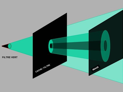
IMAGE IMAGE IMAGE
CACHE CACHE / / FILTRE FILTRE
FILTRE VERT

Dans un système linéaire, mesurer
l’amplitude du signal de sortie du système
pour une amplitude d’entrée constante
(l’approche de l’ingénieur) est équivalent à
mesurer l’amplitude entrante requise afin
d’obtenir un signal de sortie constant
(l’approche du psychophysicien).

LUMINANCE
BANDE DE MACH
ESPACE
BRILLANCE

L’INHIBITION LATERALE
Hartline, H.K., Wagne, H.G. & Ratliff, F.
(1956). INHIBITION IN THE EYE OF
LIMULUS. Journal of General Physiology 39,
651-673.

BRILLANCE
LUMINANCE
One version of the Craik-O’Brien-Cornsweet effect.

An illusion by Vasarely, left, and a
bandpass filtered version, right.

The simultaneous contrast effect.

Un ‘seul et même’ 1 CR pourrait donc
expliquer la fonction de transfert de
contraste humaine…
__________
1C.-à-d. une seule taile de CR.

FONCTION DE TRANSFERT DE
MODULATION
et
REPONSE IMPULSIONNELLE

Inhibition centre-pourtour.

Dans un système linéaire et rétinotopique, la représentation d’un ensemble de points / image par
un seul neurone est strictement identique à la représentation d’un point dans l’espace physique
par l’ensemble des neurones qui le traitent.

CHAMP RECEPTEUR
REPONSE IMPULSIONELLE

( ) = ΣE( l − k) • CR(k)
S k
l=+∞
l=−∞
( ) = ΣE() l • CR(l − k)
S k
l=+∞
l=−∞

CONVOLUTION
1 1 1 1 2 3 4 5 5 5 5
-1 3 -1
Σ
Champ récepteur
( ) E ∗h
= ∫ +∞ −∞
S X
= E(X − x) • h(x) dx
1 1 0 2 3 4 6 5 5
E(X) = Entrée (fct. de X)
S(X) = Sortie (fct. de X)
CR = h(x) = Réponse Implle (fct. de x)
Σ
1 1 1 1 2 3 4 5 5 5 5
-1 3 -1
Réponse impulsionnelle
3 -1
-1 3 -1
-1 3 -1
-1 3 -1
-2 6 -2
-3 9 -3
-4 12 -4
-5 15 -5
-5 15 -5
E ∗h
= E(X) • h(X − x)
-5 15 -5
-5 15
( ) ∫ +∞ −∞
S X
= dx
1 1 0 2 3 4 6 5 5

Campbell & Robson, 1968

Campbell & Robson, 1968

Campbell & Robson, 1968
4 ⎡ 1 1
⎤
I(fx) carré = 1+ C
⎢
sin( π fx) + sin(3π fx) + sin(5π fx) + L
π ⎣ 3 5
⎥
⎦
Réponse / sensibilité prédite pour un réseau carré de fréquence fx et de
contraste C :
4 ⎡
1 1
⎤
R(fx) carré = 1+ C
⎢
Rfx sin( π fx) + R3fx sin(3π fx) + R5fx
sin(5π fx) + L
3 5
⎥
sin sin sin
π ⎣ ⎦

Campbell & Robson, 1968
Mesuré
Prédit
4/π

Campbell & Robson, 1968

Il y aurait donc plusieurs tailles
de CRs ou, ce qui revient au
même, plusieurs filtres centrés
sur plusieurs fréquences
− + − − + −

1969
1969

Wilson, H.R & Bergen, J.R. (1979). A
four mechanisms model for spatial
vision. Vision Research 19, 19-32.

REPRESENTATION ‘MULTIECHELLE’ DE CHAQUE POINT RETINIEN
FOVEA
Excentricité

Un « canal » d’Orientation…

Les « canaux » / filtres rétiniens dans le domaine
chromatique (longueur d’onde) - normalisés

Les « canaux » / filtres
rétiniens dans le domaine
chromatique (longueur d’onde)
– non-normalisés

Description of the ideal observer in a 2-feature trial in Experiment 2. First the ideal observer computes the
ideal template, which is the difference between the target and the distractor. Then the ideal observer
cross-correlates (takes the dot product)* this difference with the stimuli at each location. The location with
the maximum dot product value is the stimulus that best matches the template, and is chosen as the
target location.
_______________________
*x i y j [template] x i y j [stimulus]
Shimozaki, S.S., Eckstein, M.P. & Abbey, C.K. (2002). Stimulus information contaminates summation
tests of independent neural representations of features. Journal of Vision, 2, 354-370.

Schematic of the linear summation model. A 2-feature search from Experiment 2 is depicted with the
target in the left locations. An independent response is generated for both spatial frequency and
orientation at each location. These responses are weighted by the d’ for the particular feature and
summed. The location with the maximal weighted linear response (xt-linear or xd-linear) is chosen as the
target location.
Shimozaki, S.S., Eckstein, M.P. & Abbey, C.K. (2002). Stimulus information contaminates summation
tests of independent neural representations of features. Journal of Vision, 2, 354-370.

Feature 2
Geometric description of linear summation. Each axis represents the sensitivity to each feature in d’ units.
The sensitivity when both feature cues are available is equal to the Euclidean vector sum of the individual
sensitivities. The orthogonal axes represent independence of the two features.
Shimozaki, S.S., Eckstein, M.P. & Abbey, C.K. (2002). Stimulus information contaminates summation
tests of independent neural representations of features. Journal of Vision, 2, 354-370.

Schematic of the probability summation model. A 2-feature search from Experiment 2 is depicted with the
target in the left locations. An independent response is generated for both spatial frequency and
orientation at each location, and the location with the maximal featural response is chosen as the target
location.
Shimozaki, S.S., Eckstein, M.P. & Abbey, C.K. (2002). Stimulus information contaminates summation
tests of independent neural representations of features. Journal of Vision, 2, 354-370.

CANAUX, BRUIT
et
LA THÉORIE DE LA DÉTECTION DU SIGNAL

Le principe de l’UNIVARIANCE
Réponse (s/s ou autre)
Intensité ou « qualité » du Stimulus
R
Intensité
«Qualité»(λ)
V

RESPONSE NORMALIZATION
Heeger, D.J. (1992) Normalization of cell responses in cat striate cortex. Visual Neuroscience, 9, 181-197.

LE MODÉLE STANDARD : LA THÉORIE DE LA DÉTECTION DU SIGNAL
RESPONSE
L
RESPONSE
L
RESPONSE
λ
λ
λ
R
«COULEUR»
V
R
«COULEUR»
V
ΔR
ΔR
PROBAB.
σ
PROBAB.
σ
CONTINUUM SENSORIEL (R-V)
CONTINUUM SENSORIEL (R-V)
d’ n’est pas mesurable
d’= ΔR σ

CANAUX & PROBABILITÉ DE RÉPONSE
LE PLUS RÉPONDANT GAGNE
RÉPONSE
p Max
p min
REPONSE (e.g. s/s)
R V
p(s/s)
p min
x p max
pmin x p max
R V
p[R(Y/G) largest]

CANAUX & PROBABILITÉ DE RÉPONSE
« OFF-LOOKING » CHANNEL
RÉPONSE
REPONSE (e.g. s/s)
R
V
p(s/s)
REPONSE (e.g. s/s)
R
V
p(s/s)