these simulation numerique et modelisation de l'ecoulement autour ...

ARTIFICIAL VISCOSITY MODELS
A.2.1
The Jameson sensor
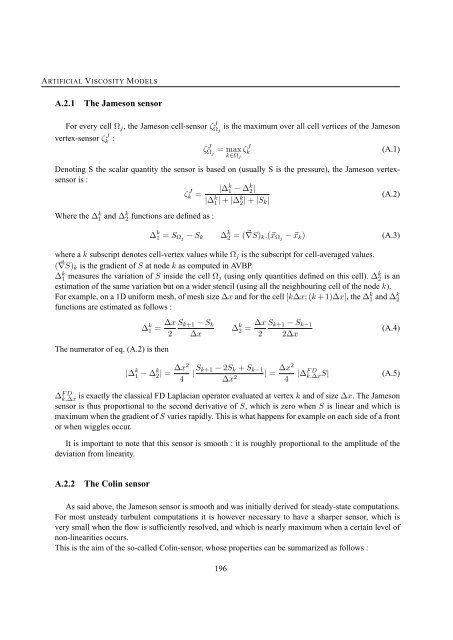
For every cell Ω j , the Jameson cell-sensor ζ J Ω j
is the maximum over all cell vertices of the Jameson
vertex-sensor ζ J k :
ζ J Ω j
= max
k∈Ω j
ζ J k
(A.1)
Denoting S the scalar quantity the sensor is based on (usually S is the pressure), the Jameson vertexsensor
is :
ζk J |∆ k 1
=
− ∆k 2 |
|∆ k 1 | + |∆k 2 | + |S (A.2)
k|
Where the ∆ k 1 and ∆k 2 functions are defined as :
∆ k 1 = S Ωj − S k ∆ k 2 = ( ⃗ ∇S) k .(⃗x Ωj − ⃗x k ) (A.3)
where a k subscript denotes cell-vertex values while Ω j is the subscript for cell-averaged values.
( ∇S) ⃗ k is the gradient of S at node k as computed in AVBP.
∆ k 1 measures the variation of S inside the cell Ω j (using only quantities defined on this cell). ∆ k 2 is an
estimation of the same variation but on a wider stencil (using all the neighbouring cell of the node k).
For example, on a 1D uniform mesh, of mesh size ∆x and for the cell [k∆x; (k + 1)∆x], the ∆ k 1 and ∆k 2
functions are estimated as follows :
The numerator of eq. (A.2) is then
∆ k 1 = ∆x S k+1 − S k
2 ∆x
∆ k 2 = ∆x S k+1 − S k−1
2 2∆x
(A.4)
|∆ k 1 − ∆ k 2| = ∆x2
4
| S k+1 − 2S k + S k−1
∆x 2 | = ∆x2
4
|∆ F D
k,∆xS|
(A.5)
is exactly the classical FD Laplacian operator evaluated at vertex k and of size ∆x. The Jameson
sensor is thus proportional to the second derivative of S, which is zero when S is linear and which is
maximum when the gradient of S varies rapidly. This is what happens for example on each side of a front
or when wiggles occur.
∆ F k,∆x D
It is important to note that this sensor is smooth : it is roughly proportional to the amplitude of the
deviation from linearity.
A.2.2
The Colin sensor
As said above, the Jameson sensor is smooth and was initially derived for steady-state computations.
For most unsteady turbulent computations it is however necessary to have a sharper sensor, which is
very small when the flow is sufficiently resolved, and which is nearly maximum when a certain level of
non-linearities occurs.
This is the aim of the so-called Colin-sensor, whose properties can be summarized as follows :
196