these simulation numerique et modelisation de l'ecoulement autour ...
these simulation numerique et modelisation de l'ecoulement autour ...
these simulation numerique et modelisation de l'ecoulement autour ...

You also want an ePaper? Increase the reach of your titles
YUMPU automatically turns print PDFs into web optimized ePapers that Google loves.
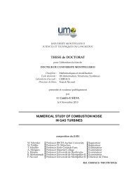
V<br />
U<br />
σ V inj<br />
j<strong>et</strong> cotan(α′ )<br />
V<br />
U<br />
σ V suc<br />
j<strong>et</strong> cotan(β ′ )<br />
σ V inj<br />
j<strong>et</strong><br />
0 0<br />
S W<br />
INJECTION SIDE<br />
S W<br />
σ Vj<strong>et</strong><br />
suc<br />
0 0<br />
S W<br />
SUCTION SIDE<br />
S W<br />
Figure 7. Representation of the uniform mo<strong>de</strong>l <strong>de</strong>scribed by Eq. 10 to 13: UM2.<br />
negligible b<strong>et</strong>ween the intermediate mo<strong>de</strong>l and the UM2 mo<strong>de</strong>l.<br />
C. Implementation of the LES mo<strong>de</strong>ls<br />
The mo<strong>de</strong>ls proposed in section III.B, UM1 and UM2, are implemented in the AVBP co<strong>de</strong><br />
(section IIA).<br />
To make the coupling easier, one assumes that the surface meshes on the injection and the<br />
suction si<strong>de</strong>s coinci<strong>de</strong> (see Fig.8). To d<strong>et</strong>ermine the operating conditions at a liner point, only<br />
the values at this no<strong>de</strong> and at the corresponding no<strong>de</strong> on the other si<strong>de</strong> of the plate (same<br />
streamwise and spanwise coordinates on the other si<strong>de</strong>) are used. At each iteration, the mass<br />
flow rate per surface unit through the plate, ϕ, is computed from the pressure drop across<br />
the liner, assessed as the difference b<strong>et</strong>ween the nodal pressures P inj and P suc (see Fig.8).<br />
For doing so, ϕ is related to the micro-j<strong>et</strong>s velocity V j , viz. ϕ = ρV j sin(α) σ. Introducing<br />
1<br />
the discharge coefficient C D to express V j as a function of ∆P = P suc − P inj , viz. ρV 2 =<br />
√<br />
2<br />
C 2 D ∆P, the mass flow rate per unit wall surface is then ϕ = sin(α) σ 2ρ suc C 2 D ∆P. Note<br />
that in this latter relation, the <strong>de</strong>nsity is assessed at the suction si<strong>de</strong>, viz. ρ = ρ suc .<br />
Once ϕ is known, the following quantities are imposed:<br />
• at the suction si<strong>de</strong>: the only variable imposed is the normal velocity, computed as<br />
V suc<br />
W<br />
= ϕ ρ suc<br />
. As only one quantity can be imposed for an outl<strong>et</strong> boundary condition,<br />
both uniform mo<strong>de</strong>ls are implemented with the same boundary conditions for the<br />
suction si<strong>de</strong>, corresponding to the UM2 mo<strong>de</strong>l (Eq. 12 and 13).<br />
• at the injection si<strong>de</strong>: ρ is d<strong>et</strong>ermined from the temperature T s uc (assumed to be also<br />
the fluid temperature at the hole outl<strong>et</strong>) and the pressure P inj . Then the normal<br />
velocity is V inj<br />
W<br />
UM1 and U inj<br />
W<br />
= ϕ ρ inj<br />
and the streamwise velocity is s<strong>et</strong> to U inj<br />
W<br />
= V inj<br />
W<br />
cotan(α′ ) in UM2.<br />
= V inj<br />
W<br />
cotan(α) in<br />
The number of imposed quantities corresponds to what is usually done for classical inl<strong>et</strong>s/outl<strong>et</strong>s.<br />
16 of 26