these simulation numerique et modelisation de l'ecoulement autour ...

LES of a bi-periodic turbulent flow with effusion 33
Figure 21. Reynolds stress and velocity fluctuations at the hole outlet. (a): Contours of the
the Reynolds stress −ρ(U) t (V ) tt , (b): Contours of the streamwise root mean square velocity,
(c): Contours of the vertical root mean square velocity.
0.0
vertical position
-0.5
-1.0
-1.5
-2.0
40
60
80
Flow/Jet angle (deg.)
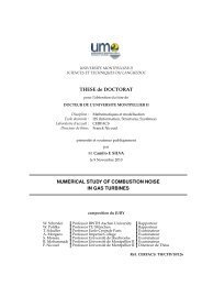
Figure 22. Flow angle ( ) and jet angle ( ) as a function of the vertical position:
y = −2 d is the position of the hole inlet and y = 0, the position of the hole outlet. The
geometric hole angle (α g = 30 ◦ ) is also plotted ( ).
100
especially near the centre of the hole outlet where the turbulence intensity is as large
as 30 %: figure 21(b,c) shows that streamwise and vertical root mean square velocity
can reach 20 % of the bulk velocity in the hole. However, as shown in figure 21(a), the
Reynolds stress −ρ(U) t (V ) tt is positive in the hole centre and negative in the wall region
so that its contribution to equation 5.4 is very small.
In the previous approximation of the momentum flux, the V ts term is easy to estimate,
as the mass flow rate is supposed to be known. On the contrary, the time-space average
over the hole inlet/outlet of the streamwise velocity is not known a priori. One way
to proceed is to relate these two quantities via the flow angle α defined as the angle
between the (x, z)-plane and the time-averaged, plane-averaged velocity vector. In other
words, the flow angle is such that V ts = U ts tan α: if the plane-averaged velocity vector
is vertical, the flow angle is 90 ◦ and if it is along the streamwise direction, α = 0 ◦ . Of
course, a natural modelling idea would be to assume that α is imposed by the geometrical
characteristics of the aperture (recall that the geometrical angle is α g = 30 ◦ ). In order
to test this simple idea, figure 22 shows the evolution of the flow angle in the hole as a
function of the vertical coordinate (solid line). The hole inlet (suction wall) is located at
y = −2 d and the hole outlet (injection wall) is at y = 0. The averaged orientation of
the flow within the hole changes along the aperture and proves to be different from the
hole angle. At the inlet of the hole, α is approximately 55 ◦ , almost twice as large as the