Manuscrit en Français - Institut de Physique du Globe de Paris
Manuscrit en Français - Institut de Physique du Globe de Paris
Manuscrit en Français - Institut de Physique du Globe de Paris

Create successful ePaper yourself
Turn your PDF publications into a flip-book with our unique Google optimized e-Paper software.
INSTITUT DE PHYSIQUE DU GLOBE DE PARIS<br />
Université <strong>Paris</strong> Di<strong>de</strong>rot<br />
Thèse <strong>de</strong> doctorat<br />
Dynamique <strong>de</strong>s instabilités gravitaires<br />
par modélisation et télédétection:<br />
Applications aux exemples marti<strong>en</strong>s<br />
ANTOINE LUCAS<br />
- 30 mars 2010 -
Dynamique <strong>de</strong>s instabilités gravitaires<br />
par modélisation et télédétection:<br />
Applications aux exemples marti<strong>en</strong>s<br />
Thèse <strong>de</strong> doctorat<br />
Prés<strong>en</strong>tée par<br />
Antoine Lucas<br />
pour l’obt<strong>en</strong>tion <strong>du</strong> titre <strong>de</strong> docteur <strong>de</strong> l’<strong>Institut</strong> <strong>de</strong> <strong>Physique</strong> <strong>du</strong> <strong>Globe</strong> <strong>de</strong> <strong>Paris</strong><br />
(Spécialité Géophysique planétaire)<br />
Devant le jury composé <strong>de</strong><br />
ANNE MANGENEY M.C. HDR IPGP, Université <strong>Paris</strong>-Di<strong>de</strong>rot (Directrice)<br />
DANIEL MÈGE M.C. HDR LPGN, Université <strong>de</strong> Nantes (Co-Directeur)<br />
PHILLIPE LOGNONNÉ Prof. IPGP, Université <strong>Paris</strong>-Di<strong>de</strong>rot (Examinateur)<br />
JEAN-PHILLIPE MALET C.R. CNRS EOST (Examinateur)<br />
FRANÇOIS COSTARD D.R. CNRS, Université <strong>Paris</strong> Sud, Orsay (Rapporteur)<br />
OLDRICH HUNGR Prof. University of British Columbia, Canada (Rapporteur)<br />
30 mars 2010
v<br />
Remerciem<strong>en</strong>ts<br />
De San Diego à Hong-Kong <strong>en</strong> passant par Nantes, Londres, Houston, Berlin et même Mars, ce<br />
travail <strong>de</strong> thèse m’a avant tout permis <strong>de</strong> voyager intellectuellem<strong>en</strong>t. C’est avec une imm<strong>en</strong>se<br />
sincérité que je remercie mes <strong>de</strong>ux directeurs <strong>de</strong> thèse, Anne Mang<strong>en</strong>ey et Daniel Mège<br />
pour m’avoir accordé leur confiance et permis <strong>de</strong> m<strong>en</strong>er à bi<strong>en</strong> ce travail dans d’excell<strong>en</strong>tes<br />
conditions. J’ai eu beaucoup <strong>de</strong> plaisir à travailler avec eux et suivre leurs conseils toujours<br />
pertin<strong>en</strong>ts et justifiés. C’est avec un grand plaisir que je continuerai à collaborer avec eux.<br />
Merci au jury composé <strong>de</strong> Jean-Philippe Malet, Philippe Lognonnée, François Costard et<br />
Oldrich Hungr pour avoir accepté d’évaluer ce travail.<br />
Je remercie toute l’équipe <strong>de</strong> sismologie pour son accueil, sa bonne humeur et sa disponibilité.<br />
Je ti<strong>en</strong>s à saluer tout particulièrem<strong>en</strong>t Pascal Favreau pour m’avoir initié à la sismologie.<br />
Un grand merci à G<strong>en</strong>eviève Moguilny et Patrick Stoclet pour leur souti<strong>en</strong> technique indisp<strong>en</strong>sable,<br />
Sylvie Contamina pour son ai<strong>de</strong> administrative sans faille. Merci à mes collègues<br />
<strong>de</strong> bureau, Diego, Adri<strong>en</strong>, Xavier, Gaël, Clém<strong>en</strong>t, Sébasti<strong>en</strong>, Stéphanie, Juli<strong>en</strong>, Alexandre,<br />
Laur<strong>en</strong>t, Matthieu, Mathieu, Huong, Élodie et les autres. . .Je t<strong>en</strong>ais égalem<strong>en</strong>t à adresser mes<br />
remerciem<strong>en</strong>ts aux sableuses et tractopelles <strong>du</strong> chantier <strong>de</strong> Jussieu pour m’avoir accompagné<br />
p<strong>en</strong>dant ces trois années <strong>de</strong> leur douce mélodie.<br />
Je remercie le laboratoire <strong>de</strong> planétologie et géodynamique <strong>de</strong> Nantes pour m’avoir, une<br />
secon<strong>de</strong> fois, accueilli p<strong>en</strong>dant sept mois. Merci à Stéphane Le Mouélic, Olivier Bourgeois,<br />
Christophe Sotin, Nicolas Mangold et Christophe Desaillie pour leur souti<strong>en</strong> sci<strong>en</strong>tifique et<br />
technique.<br />
Je t<strong>en</strong>ais égalem<strong>en</strong>t à remercier Jan Peter Muller et Peter Grindrod <strong>de</strong> UCL pour m’avoir donné<br />
accès à la station stéréo et ainsi nous permettre d’être la première équipe <strong>en</strong> Europe à utiliser<br />
les MNT HiRISE.<br />
Je salue les g<strong>en</strong>s qui, <strong>de</strong> près ou <strong>de</strong> loin, ont subi les dommages collatéraux d’un thésard <strong>en</strong><br />
pleine rédaction : Bertrand, B<strong>en</strong>oît, David, Fouk, Nico, Marx Dormoy & Co (Cor<strong>en</strong>tin, Juli<strong>en</strong>,<br />
Marie, Thomas, Sylvain(s), B<strong>en</strong>J, Pauline, Valérie, Jérémie. . .), la promo 2004 <strong>de</strong>s gogologues<br />
<strong>de</strong> Nantes.<br />
Évi<strong>de</strong>mm<strong>en</strong>t, ce travail n’aurait pas pu être m<strong>en</strong>é sans la participation <strong>de</strong> mes par<strong>en</strong>ts, il y a 28<br />
ans déjà. Ils ont, sans faille aucune, toujours su me sout<strong>en</strong>ir et m’<strong>en</strong>courager dans mes choix.<br />
Merci à ma famille égalem<strong>en</strong>t pour avoir accepté mes abs<strong>en</strong>ces, certains week-<strong>en</strong>ds passés au<br />
labo et surtout pour tout le reste.<br />
Enfin, un imm<strong>en</strong>se merci à Nadaya pour son souti<strong>en</strong> quotidi<strong>en</strong> <strong>de</strong>puis la Californie p<strong>en</strong>dant ces<br />
longs mois.
Résumé<br />
Les instabilités gravitaires contribu<strong>en</strong>t aux processus <strong>de</strong> transport <strong>de</strong> matière à la surface <strong>de</strong>s planètes et<br />
constitu<strong>en</strong>t <strong>de</strong>s risques importants pour les populations sur Terre. Afin d’apporter <strong>de</strong>s contraintes sur la<br />
dynamique <strong>de</strong>s instabilités gravitaires, notre étu<strong>de</strong> se base sur le couplage <strong>en</strong>tre simulation numérique<br />
et analyse <strong>de</strong>s données par télédétection. Le modèle utilisé s’est montré capable <strong>de</strong> repro<strong>du</strong>ire <strong>de</strong>s observations<br />
<strong>en</strong> laboratoire ainsi que la dynamique <strong>en</strong>registrée par <strong>de</strong>s signaux sismiques pour un exemple<br />
terrestre. En outre, nous avons développé une métho<strong>de</strong> <strong>de</strong> reconstruction topographique pré-glissem<strong>en</strong>t<br />
<strong>en</strong> utilisant les données satellitaires afin d’étudier les effets <strong>de</strong>s conditions initiales. En effet, la distance<br />
d’arrêt (runout) <strong>de</strong>s dépôts est très largem<strong>en</strong>t utilisée dans l’analyse <strong>de</strong> la dynamique <strong>de</strong>s glissem<strong>en</strong>ts <strong>de</strong><br />
terrain ainsi que dans la calibration <strong>de</strong>s paramètres rhéologiques impliqués dans la modélisation, et ce<br />
malgré les incertitu<strong>de</strong>s sur la géométrie initiale. Nous montrons par <strong>de</strong>s tests théoriques que le runout<br />
est faiblem<strong>en</strong>t affecté par la géométrie <strong>du</strong> plan <strong>de</strong> rupture. Au contraire, l’ext<strong>en</strong>sion latérale se révèle<br />
être contrôlée par la géométrie initiale ce qui fourni un cadre unique pour remonter égalem<strong>en</strong>t au volume<br />
initial. L’application aux exemples marti<strong>en</strong>s apporte <strong>de</strong>s contraintes sur les conditions <strong>de</strong> mise <strong>en</strong> place et<br />
ouvre <strong>de</strong> nouvelles perspectives pour la compréh<strong>en</strong>sion <strong>de</strong> la dynamique <strong>de</strong> ces processus. En outre, nous<br />
intro<strong>du</strong>isons un nouveau paramètre <strong>de</strong> dissipation empirique indép<strong>en</strong>dant <strong>de</strong> la topographie permettant,<br />
sans calibration, <strong>de</strong> retrouver par la simulation la bonne distance <strong>de</strong> runout dans un contexte géologique<br />
donné.<br />
vii
Abstract<br />
Slope instabilities take part in weathering and transport processes at the surface. The runout distance is<br />
ext<strong>en</strong>sively used in analysis of landsli<strong>de</strong> dynamics and in the calibration of the rheological parameters<br />
involved in numerical mo<strong>de</strong>lling. However, the unknown impact of the uncertainty in the shape of the<br />
initial released mass on the runout distance and on the overall shape of the <strong>de</strong>posit questions the relevance<br />
of these approaches. In<strong>de</strong>ed, the shape of the initial scar is g<strong>en</strong>erally unknown in real cases. Our study<br />
is based on numerical simulations coupled with remote s<strong>en</strong>sing data analysis. The mo<strong>de</strong>l used in this<br />
study has be<strong>en</strong> int<strong>en</strong>sively compared with laboratory experim<strong>en</strong>ts and well constrained natural cases<br />
in or<strong>de</strong>r to establish its range of use. We have also <strong>de</strong>veloped a pre-ev<strong>en</strong>t topographic reconstruction<br />
method using remote s<strong>en</strong>sing data allowing the study of the topographic and initial failure plane geometry<br />
effects. We show that the runout distance is a robust parameter that is only poorly affected by the initial<br />
scar geometry. On the contrary, the ext<strong>en</strong>t of the <strong>de</strong>posits perp<strong>en</strong>dicular to the main mass displacem<strong>en</strong>t<br />
direction is shown to be controlled by the scar geometry, providing a unique tool to retrieve information of<br />
the initial failure geometry, as well as on the released volume. A feedback analysis of Martian landsli<strong>de</strong>s<br />
shows excell<strong>en</strong>t agreem<strong>en</strong>t betwe<strong>en</strong> numerical results and geomorphological evid<strong>en</strong>ce, providing insight<br />
into the initial landsliding conditions. In addition, we intro<strong>du</strong>ce a new empirical dissipation parameter<br />
allowing a good prediction of the runout in the simulation without any calibration for a giv<strong>en</strong> geological<br />
context.<br />
viii
ix<br />
Notations et liste <strong>de</strong> symboles<br />
Sont regroupées ici les notations mathématiques employées dans le manuscript. Les scalairs sont<br />
notées <strong>en</strong> italique x. Les vecteurs 2D sont notés <strong>en</strong> gras c et les vecteurs 3D avec une flèche ⃗n. Les<br />
notations (x, y, z) ne sont pas réservées aux coordonnées cartési<strong>en</strong>nes. La lettre t est réservée pour<br />
le temps. La notation ∂ x (.) désigne la dérivée partielle première <strong>de</strong> (.) par rapport à x. La notation<br />
∇ X z désigne la dérivée partielle première <strong>de</strong> z dans le référ<strong>en</strong>tiel X.<br />
Symboles Latins<br />
dx<br />
dy<br />
incrém<strong>en</strong>t <strong>en</strong> x<br />
incrém<strong>en</strong>t <strong>en</strong> y<br />
f, F , F force<br />
g<br />
g<br />
h<br />
H max<br />
H 0 ,H i<br />
H f<br />
¯h<br />
h n i,j<br />
m<br />
p<br />
t<br />
constante <strong>de</strong> l’accélération <strong>de</strong> la gravité<br />
vecteur <strong>de</strong> l’accélération <strong>de</strong> la gravité<br />
épaisseur <strong>de</strong> l’avalanche<br />
hauteur maximale <strong>de</strong> l’avalanche<br />
Hauteur initiale <strong>de</strong> l’avalanche<br />
Hauteur finale <strong>de</strong> l’avalanche<br />
valeur moy<strong>en</strong>ne <strong>de</strong> h<br />
valeur numérique <strong>de</strong> h au point i, j et à l’incrém<strong>en</strong>t n<br />
Masse d’un corps<br />
Pression<br />
temps<br />
T<br />
Symboles Grecs<br />
δ<br />
∆x<br />
ρ<br />
Angle <strong>de</strong> friction<br />
Incrém<strong>en</strong>t <strong>de</strong> x <strong>en</strong> différ<strong>en</strong>ce finie<br />
D<strong>en</strong>sité
Table <strong>de</strong>s matières<br />
1 Intro<strong>du</strong>ction 1<br />
1.1 Phénoménologie d’un processus géophysique majeur . . . . . . . . . . . . . . . . . 1<br />
1.2 Résulats expérim<strong>en</strong>taux et numériques . . . . . . . . . . . . . . . . . . . . . . . . . 4<br />
1.3 Les exemples marti<strong>en</strong>s . . . . . . . . . . . . . . . . . . . . . . . . . . . . . . . . . 9<br />
1.4 Objectifs . . . . . . . . . . . . . . . . . . . . . . . . . . . . . . . . . . . . . . . . . 13<br />
2 Modélisation numérique d’avalanches granulaires 17<br />
2.1 Description <strong>du</strong> modèle . . . . . . . . . . . . . . . . . . . . . . . . . . . . . . . . . 17<br />
2.2 Évolution <strong>du</strong> co<strong>de</strong> pour une utilisation <strong>en</strong> géophysique . . . . . . . . . . . . . . . . 22<br />
2.2.1 Assimilation <strong>de</strong>s données . . . . . . . . . . . . . . . . . . . . . . . . . . . . 27<br />
2.3 Confrontation <strong>du</strong> modèle . . . . . . . . . . . . . . . . . . . . . . . . . . . . . . . . 29<br />
2.3.1 Estimation <strong>de</strong> la dissipation numérique . . . . . . . . . . . . . . . . . . . . . 29<br />
2.3.2 Confrontation aux expéri<strong>en</strong>ces <strong>en</strong> laboratoire . . . . . . . . . . . . . . . . . 32<br />
2.3.3 Confrontation à <strong>de</strong>s exemples naturels . . . . . . . . . . . . . . . . . . . . . 37<br />
2.4 Conclusions . . . . . . . . . . . . . . . . . . . . . . . . . . . . . . . . . . . . . . . 50<br />
3 Dynamique <strong>de</strong>s glissem<strong>en</strong>ts <strong>de</strong> terrain par sismologie 53<br />
3.1 Motivations et contexte . . . . . . . . . . . . . . . . . . . . . . . . . . . . . . . . . 53<br />
3.2 Dynamique et paramètres <strong>de</strong> friction . . . . . . . . . . . . . . . . . . . . . . . . . . 55<br />
3.3 Génération d’un signal sismique <strong>de</strong>puis une force ponctuelle . . . . . . . . . . . . . 60<br />
3.3.1 Résultats . . . . . . . . . . . . . . . . . . . . . . . . . . . . . . . . . . . . 61<br />
3.4 Conclusions . . . . . . . . . . . . . . . . . . . . . . . . . . . . . . . . . . . . . . . 70<br />
4 Données et Méthodologies 73<br />
4.1 Intro<strong>du</strong>ction . . . . . . . . . . . . . . . . . . . . . . . . . . . . . . . . . . . . . . . 73<br />
4.2 Imagerie . . . . . . . . . . . . . . . . . . . . . . . . . . . . . . . . . . . . . . . . . 74<br />
xi
xii<br />
TABLE DES MATIÈRES<br />
4.2.1 Imagerie visible . . . . . . . . . . . . . . . . . . . . . . . . . . . . . . . . . 74<br />
4.2.2 Imagerie Infrarouge . . . . . . . . . . . . . . . . . . . . . . . . . . . . . . . 75<br />
4.3 Traitem<strong>en</strong>t <strong>de</strong>s images . . . . . . . . . . . . . . . . . . . . . . . . . . . . . . . . . . 80<br />
4.3.1 Cont<strong>en</strong>u <strong>de</strong>s données . . . . . . . . . . . . . . . . . . . . . . . . . . . . . . 80<br />
4.3.2 Calibration radiométrique et correction <strong>du</strong> bruit . . . . . . . . . . . . . . . . 82<br />
4.4 Extraction topographique . . . . . . . . . . . . . . . . . . . . . . . . . . . . . . . . 88<br />
4.4.1 Intro<strong>du</strong>ction . . . . . . . . . . . . . . . . . . . . . . . . . . . . . . . . . . . 88<br />
4.4.2 Préparation et calibration <strong>de</strong>s données . . . . . . . . . . . . . . . . . . . . . 91<br />
4.4.3 Id<strong>en</strong>tification <strong>de</strong>s points homologues . . . . . . . . . . . . . . . . . . . . . . 92<br />
4.4.4 Validation <strong>du</strong> modèle numérique <strong>de</strong> terrain . . . . . . . . . . . . . . . . . . . 95<br />
4.4.5 Métho<strong>de</strong>s alternatives pour l’extraction topographique . . . . . . . . . . . . 100<br />
4.5 Méthodologie <strong>de</strong> reconstruction topographique pré-glissem<strong>en</strong>t . . . . . . . . . . . . 104<br />
4.5.1 Id<strong>en</strong>tification <strong>de</strong>s dépôts par télédétection . . . . . . . . . . . . . . . . . . . 104<br />
4.5.2 Modification vectorielle <strong>de</strong> l’information topographique . . . . . . . . . . . 104<br />
4.5.3 Régularisation <strong>de</strong> l’information topographique par estimation optimale . . . . 105<br />
4.6 Conclusions . . . . . . . . . . . . . . . . . . . . . . . . . . . . . . . . . . . . . . . 109<br />
5 Écoulem<strong>en</strong>ts granulaires marti<strong>en</strong>s 111<br />
5.1 Motivations . . . . . . . . . . . . . . . . . . . . . . . . . . . . . . . . . . . . . . . 111<br />
5.2 Ravines sinueuses et implications rhéologiques . . . . . . . . . . . . . . . . . . . . 112<br />
5.2.1 Expéri<strong>en</strong>ces numériques sur topographies modèles . . . . . . . . . . . . . . 115<br />
5.2.2 Bilan . . . . . . . . . . . . . . . . . . . . . . . . . . . . . . . . . . . . . . 129<br />
5.3 Ravines marti<strong>en</strong>nes digitées . . . . . . . . . . . . . . . . . . . . . . . . . . . . . . . 130<br />
5.4 Écoulem<strong>en</strong>t <strong>de</strong> type « slope streaks » . . . . . . . . . . . . . . . . . . . . . . . . . . 135<br />
5.5 Conclusions . . . . . . . . . . . . . . . . . . . . . . . . . . . . . . . . . . . . . . . 140<br />
6 Paramétrisation <strong>de</strong> la dissipation moy<strong>en</strong>ne 145<br />
6.1 Intro<strong>du</strong>ction . . . . . . . . . . . . . . . . . . . . . . . . . . . . . . . . . . . . . . . 152<br />
6.2 Résultats expérim<strong>en</strong>taux et numériques . . . . . . . . . . . . . . . . . . . . . . . . . 153<br />
6.3 Effets <strong>de</strong> la p<strong>en</strong>te et <strong>de</strong> la friction sur topographie 2D . . . . . . . . . . . . . . . . . 155<br />
6.4 Simulation sur topographie réalistes 3D . . . . . . . . . . . . . . . . . . . . . . . . 157<br />
6.4.1 Reconstruction <strong>de</strong> la topographie . . . . . . . . . . . . . . . . . . . . . . . . 157
TABLE DES MATIÈRES<br />
xiii<br />
6.4.2 Résultats et comparaisons avec les observations à l’échelle MOLA . . . . . . 158<br />
6.5 Vers une nouvelle mobilité, facteur <strong>de</strong> déplacem<strong>en</strong>t intrinsèque . . . . . . . . . . . . 158<br />
6.6 Conclusions . . . . . . . . . . . . . . . . . . . . . . . . . . . . . . . . . . . . . . . 160<br />
7 Effets <strong>de</strong> la géométrie <strong>de</strong> la rupture sur la dynamique 163<br />
7.1 Intro<strong>du</strong>ction . . . . . . . . . . . . . . . . . . . . . . . . . . . . . . . . . . . . . . . 167<br />
7.2 Cas d’étu<strong>de</strong> et contexte géologique . . . . . . . . . . . . . . . . . . . . . . . . . . . 170<br />
7.3 Données et méthodologie . . . . . . . . . . . . . . . . . . . . . . . . . . . . . . . . 174<br />
7.3.1 Id<strong>en</strong>tification <strong>de</strong>s dépôts . . . . . . . . . . . . . . . . . . . . . . . . . . . . 175<br />
7.3.2 Reconstruction <strong>du</strong> MNT . . . . . . . . . . . . . . . . . . . . . . . . . . . . 175<br />
7.4 Description <strong>du</strong> modèle numérique . . . . . . . . . . . . . . . . . . . . . . . . . . . 178<br />
7.5 Tests numériques théoriques . . . . . . . . . . . . . . . . . . . . . . . . . . . . . . 180<br />
7.5.1 Écoulem<strong>en</strong>ts 2D . . . . . . . . . . . . . . . . . . . . . . . . . . . . . . . . . 180<br />
7.5.2 Écoulem<strong>en</strong>ts 3D . . . . . . . . . . . . . . . . . . . . . . . . . . . . . . . . . 183<br />
7.6 Application aux exemples marti<strong>en</strong>s . . . . . . . . . . . . . . . . . . . . . . . . . . . 186<br />
7.6.1 Propriétés frictionelles <strong>de</strong>s glissem<strong>en</strong>ts <strong>de</strong> terrain marti<strong>en</strong>s . . . . . . . . . . 186<br />
7.6.2 Dépôts simulés et géométrie <strong>du</strong> plan <strong>de</strong> rupture . . . . . . . . . . . . . . . . 191<br />
7.6.3 Bilans <strong>de</strong> masse . . . . . . . . . . . . . . . . . . . . . . . . . . . . . . . . . 192<br />
7.6.4 Implications sur les conditions <strong>de</strong> mise <strong>en</strong> place . . . . . . . . . . . . . . . . 193<br />
7.7 Conclusions . . . . . . . . . . . . . . . . . . . . . . . . . . . . . . . . . . . . . . . 195<br />
8 Conclusions et perspectives 201
Chapitre 1<br />
Intro<strong>du</strong>ction<br />
1.1 Phénoménologie d’un processus géophysique majeur<br />
Dès qu’une masse <strong>de</strong> débris rocheux se déstabilise sur une p<strong>en</strong>te, elle s’écoule sous l’effet <strong>de</strong><br />
la gravité pour s’y déposer. Ces transferts peuv<strong>en</strong>t faire interv<strong>en</strong>ir <strong>de</strong>s matériaux d’une très gran<strong>de</strong><br />
variété granulométrique (<strong>du</strong> débris aux blocs rocheux). La taille <strong>de</strong>s grains mobilisés peut aller <strong>du</strong><br />
micromètres à <strong>de</strong>s blocs <strong>de</strong> plusieurs mètres <strong>de</strong> diamètre. Aussi, la gamme <strong>de</strong> vitesse varie <strong>de</strong> plusieurs<br />
ordres <strong>de</strong> gran<strong>de</strong>ur, <strong>de</strong> quelques mm.an −1 à plusieur m.s −1 . Ces événem<strong>en</strong>ts sont parfois<br />
imperceptibles, parfois particulièrem<strong>en</strong>t <strong>de</strong>structeurs. Observés à la surface <strong>de</strong> différ<strong>en</strong>ts corps planétaires<br />
comme la Terre, la Lune, Mars ou <strong>en</strong>core les satellites <strong>de</strong> Jupiter et Saturne (figure 1.1), ces<br />
effondrem<strong>en</strong>ts gravitaires jou<strong>en</strong>t un rôle majeur dans la dynamique <strong>de</strong>s paysages et contribu<strong>en</strong>t ainsi<br />
au transport <strong>de</strong> matière à la surface <strong>de</strong>s planètes.<br />
Tributaires <strong>de</strong> mécanismes mettant <strong>en</strong> jeu <strong>de</strong>s couplages complexes <strong>en</strong>tre climat, altération, tectonique,<br />
biomasse et activités anthropiques, ces processus sont le sujet <strong>de</strong> nombreuses étu<strong>de</strong>s, à la<br />
fois <strong>en</strong> mécanique, <strong>en</strong> géophysique, <strong>en</strong> géomorphologie et <strong>en</strong> planétologie. S’intéresser à ces processus,<br />
c’est t<strong>en</strong>ter <strong>de</strong> compr<strong>en</strong>dre la dynamique <strong>de</strong> surface <strong>de</strong>s corps planétaires soli<strong>de</strong>s. En outre,<br />
l’étu<strong>de</strong> <strong>de</strong>s instabilités gravitaires constitue un cadre important pour la gestion <strong>de</strong>s risques liés à ces<br />
processus.<br />
Le nombre <strong>de</strong> terme désignant les instabilités gravitaires illustre la difficulté à définir une classification<br />
cons<strong>en</strong>suelle, car les diverses communautés qui s’y intéress<strong>en</strong>t ne s’<strong>en</strong>t<strong>en</strong>d<strong>en</strong>t pas sur les<br />
critères pertin<strong>en</strong>ts à pr<strong>en</strong>dre <strong>en</strong> compte dans la terminologie [Hungr et al., 2001]. De plus, ces écou-<br />
1
2 CHAPITRE 1. INTRODUCTION<br />
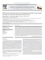
FIG. 1.1: Glissem<strong>en</strong>ts <strong>de</strong> terrain observés sur différ<strong>en</strong>ts corps planétaires comme les satellites <strong>de</strong> Jupiter (A)<br />
Callisto ,(Image SSI/Galileo, ce travail) et (B) dans la région d’Euboea Montes sur Io (topographie exagérée<br />
4 fois et extraite <strong>de</strong>puis <strong>de</strong>s images Voyager par P. Sch<strong>en</strong>k, [Sch<strong>en</strong>k and Bulmer, 1998]). (C) Exemple observé<br />
sur Japet, satellite <strong>de</strong> Saturne par la son<strong>de</strong> Cassini-Huyg<strong>en</strong>s. [Image NASA/JPL/Space Sci<strong>en</strong>ce <strong>Institut</strong>e]. (D)<br />
Glissem<strong>en</strong>t <strong>de</strong> terrain dans Ganges Chasma, sur Mars (Image HRSC drapée sur MNT HRSC, ce travail).
1.1. PHÉNOMÉNOLOGIE D’UN PROCESSUS GÉOPHYSIQUE MAJEUR 3<br />
lem<strong>en</strong>ts intrinsèquem<strong>en</strong>t non-perman<strong>en</strong>ts et non-uniformes peuv<strong>en</strong>t parfois évoluer d’un régime vers<br />
un autre, ce qui r<strong>en</strong>d l’emploi <strong>de</strong> toute classification confus. En outre, les mécanismes <strong>de</strong> décl<strong>en</strong>chem<strong>en</strong>t<br />
peuv<strong>en</strong>t être très différ<strong>en</strong>ts (séismes, précipitations, activité volcanique, phénomènes anthropiques.<br />
. .). Le comportem<strong>en</strong>t <strong>de</strong> ces écoulem<strong>en</strong>ts se montre tributaire <strong>de</strong> nombreux paramètres.<br />
Qu’il s’agisse d’éboulem<strong>en</strong>t sur un flanc volcanique, d’écoulem<strong>en</strong>t pyroclastique, d’avalanche <strong>de</strong><br />
roche ou d’écoulem<strong>en</strong>t <strong>de</strong> débris <strong>en</strong> montagne, la nature <strong>de</strong>s phénomènes physiques qui régiss<strong>en</strong>t les<br />
instabilités et les écoulem<strong>en</strong>ts gravitaires reste mal connue.<br />
Cep<strong>en</strong>dant, il convi<strong>en</strong>t <strong>de</strong> caractériser <strong>de</strong>s paramètres pertin<strong>en</strong>ts pour la <strong>de</strong>scription <strong>de</strong> la dynamique<br />
<strong>de</strong>s instabilités gravitaires (géométrie, volume, nature <strong>du</strong> matériau, rôle <strong>de</strong>s flui<strong>de</strong>s, vitesse,<br />
topographie. . .). Les étu<strong>de</strong>s sur le terrain montr<strong>en</strong>t que les instabilités gravitaires ont une gran<strong>de</strong><br />
mobilité, c’est à dire la capacité <strong>de</strong> parcourir <strong>de</strong> gran<strong>de</strong>s distances, les r<strong>en</strong>dant d’autant plus <strong>de</strong>structeurs<br />
[Heim, 1932 ; Legros, 2002]. Des relations <strong>en</strong>tre mobilité, volume, aire <strong>de</strong>s dépôts, friction<br />
appar<strong>en</strong>te ont pu être mises <strong>en</strong> évid<strong>en</strong>ce. En effet, le paramètre <strong>de</strong> mobilité, défini comme le rapport<br />
H max /L max , où H max est la hauteur <strong>de</strong> chute maximale et L max la longueur d’arrêt <strong>de</strong>s dépôts,<br />
semble dép<strong>en</strong>dre <strong>du</strong> volume (Figure 1.2a). Cette anti-corrélation suggère que la distance <strong>de</strong> parcours<br />
maximale L max (runout) est dép<strong>en</strong>dante <strong>du</strong> volume, comme le montre la Figure 1.2b. Cep<strong>en</strong>dant,<br />
une corrélation positive est observée <strong>en</strong>tre H max et L max (Figure 1.2c). L’explication proposée par<br />
Legros, [2002] est que, sur une faible p<strong>en</strong>te, une gran<strong>de</strong> augm<strong>en</strong>tation <strong>de</strong> L max correspondrait à<br />
une faible augm<strong>en</strong>tation <strong>de</strong> H max (puisque H max
4 CHAPITRE 1. INTRODUCTION<br />
FIG. 1.2: Relations <strong>en</strong>tre hauteur maximale d’effondrem<strong>en</strong>t H max , longueur d’arrêt L max et volume V pour<br />
les glissem<strong>en</strong>ts marti<strong>en</strong>s (●), les glissem<strong>en</strong>ts sous-marins (◆), les écoulem<strong>en</strong>ts <strong>de</strong> débris (×), les glissem<strong>en</strong>ts<br />
aéri<strong>en</strong>s volcaniques (△) et les glissem<strong>en</strong>ts aéri<strong>en</strong>s non volcaniques (■). (Figure modifée d’après Legros ,<br />
[2002]).<br />
giques visqueux [McEw<strong>en</strong>, 1989 ; Da<strong>de</strong> and Hupper, 1998]. La diversité <strong>de</strong>s mécanismes proposés<br />
met <strong>en</strong> lumière l’abs<strong>en</strong>ce <strong>de</strong> théorie unifiée pour expliquer cette mobilité [Legros, 2002].<br />
1.2 Résulats expérim<strong>en</strong>taux et numériques<br />
En outre, les observations sur les exemples naturels sont généralem<strong>en</strong>t effectuées après l’événem<strong>en</strong>t.<br />
Il est difficile dans ces conditions d’avoir accès aux informations concernant la dynamique <strong>de</strong><br />
l’écoulem<strong>en</strong>t. Comme nous v<strong>en</strong>ons <strong>de</strong> le voir, peu <strong>de</strong> paramètres sur le terrain permett<strong>en</strong>t ainsi <strong>de</strong><br />
vali<strong>de</strong>r la théorie. En outre, la complexité <strong>de</strong>s exemples naturels (granulométrie, géométrie, topographie.<br />
. .) r<strong>en</strong>d<strong>en</strong>t les comparaisons délicates d’un exemple à l’autre. Aussi, <strong>de</strong> nombreux travaux<br />
expérim<strong>en</strong>taux permettant <strong>de</strong> contrôler les propriétés <strong>du</strong> matériau et la géométrie <strong>du</strong> lit ont été m<strong>en</strong>és<br />
dans le but d’isoler le comportem<strong>en</strong>t <strong>de</strong> l’écoulem<strong>en</strong>t dans <strong>de</strong>s conditions définies [Gray et al, 1999 ;<br />
Grev and Hutter, 1993 ; Hutter et al, 1995 ; Pouliqu<strong>en</strong>, 1999]. Ces expéri<strong>en</strong>ces se sont montrées per-
1.2. RÉSULATS EXPÉRIMENTAUX ET NUMÉRIQUES 5<br />
tin<strong>en</strong>tes pour vali<strong>de</strong>r certaines théories [Savage and hutter, 1989]. Cep<strong>en</strong>dant, passer <strong>de</strong> l’échelle <strong>du</strong><br />
laboratoire à l’échelle <strong>du</strong> terrain pose souv<strong>en</strong>t problème.<br />
Récemm<strong>en</strong>t, <strong>de</strong>s étu<strong>de</strong>s expérim<strong>en</strong>tales et numériques ont montré que le rapport d’aspect initial<br />
a (où a = H i /L i avec H i la hauteur initiale et L i la longueur initiale) d’une masse granulaire<br />
s’effondrant sur un plan horizontal contrôlait la distance d’arrêt (ou distance <strong>de</strong> runout) <strong>de</strong>s dépôts<br />
[Lube et al., 2004 ; Lajeunesse et al., 2004 ; Mang<strong>en</strong>ey-Castelnau et al., 2005]. Les simulations<br />
numériques ont permis <strong>de</strong> montrer, <strong>en</strong> outre, que les équations ne dép<strong>en</strong>dai<strong>en</strong>t ni <strong>du</strong> volume, ni <strong>de</strong><br />
la gravité, mais seulem<strong>en</strong>t <strong>de</strong> ce rapport d’aspect initial. Ces lois d’échelles empiriques permett<strong>en</strong>t<br />
ainsi d’extrapôler les observations <strong>en</strong> laboratoire à l’échelle <strong>du</strong> terrain. Cep<strong>en</strong>dant, les expéri<strong>en</strong>ces<br />
ne permett<strong>en</strong>t pas d’avoir accès aux forces mises <strong>en</strong> jeu, ni <strong>de</strong> véritablem<strong>en</strong>t tester les conditions<br />
initiales comme la géométrie, le volume ou <strong>en</strong>core la topographie.<br />
C’est pourquoi <strong>de</strong> nombreux modèles numériques ont été développés, même si la <strong>de</strong>scription <strong>du</strong><br />
comportem<strong>en</strong>t <strong>de</strong> toutes les particules (polydisperses et hétérogènes) sur une topographie réaliste et<br />
avec la prise <strong>en</strong> compte <strong>de</strong>s intéractions év<strong>en</strong>tuelles <strong>en</strong>tre fraction soli<strong>de</strong> et fraction flui<strong>de</strong> (liée à<br />
la prés<strong>en</strong>ce <strong>de</strong> l’eau par exemple) est inaccessible aujourd’hui. Certains <strong>de</strong> ces processus sont mal<br />
compris. De plus, les temps <strong>de</strong> calcul alors <strong>de</strong>mandés sont in<strong>en</strong>visageables malgré les progrès <strong>en</strong><br />
calcul haute performance réalisés ces <strong>de</strong>rnières années. C’est pourquoi les modélisateurs s’attach<strong>en</strong>t<br />
à développer <strong>de</strong>s modèles peu coûteux <strong>en</strong> temps <strong>de</strong> calcul mais néanmoins capables <strong>de</strong> repro<strong>du</strong>ire le<br />
comportem<strong>en</strong>t moy<strong>en</strong> d’un écoulem<strong>en</strong>t granulaire afin d’étudier <strong>de</strong>s cas naturels.<br />
Il est donc nécessaire d’utiliser <strong>de</strong>s approximations sur la dynamique, la géométrie ou les lois <strong>de</strong><br />
comportem<strong>en</strong>t mécanique. La <strong>de</strong>scription <strong>du</strong> comportem<strong>en</strong>t d’un milieu granulaire à l’échelle microscopique<br />
(échelle <strong>du</strong> grain) est aujourd’hui correctem<strong>en</strong>t décrite. En revanche, le comportem<strong>en</strong>t<br />
à l’échelle <strong>de</strong> l’écoulem<strong>en</strong>t reste à ce jour mal comprise. C’est la capacité <strong>de</strong>s milieux granulaires<br />
<strong>de</strong> se comporter comme un soli<strong>de</strong> restant au repos avec une surface libre ou comme un liqui<strong>de</strong> qui<br />
s’écoule le long d’une p<strong>en</strong>te qui r<strong>en</strong>d la <strong>de</strong>scription physique difficile à cette échelle.<br />
Les modèles par élém<strong>en</strong>ts discrets décriv<strong>en</strong>t le comportem<strong>en</strong>t <strong>de</strong> chaque particule (ou grain) <strong>en</strong><br />
pr<strong>en</strong>ant <strong>en</strong> compte les interactions grain/grain. Les limites <strong>de</strong> temps <strong>de</strong> calcul impos<strong>en</strong>t néanmoins<br />
à ces modèles une taille <strong>de</strong> grain uniforme (ou quasi-uniforme) ce qui constitue une hypothèse forte<br />
au regard <strong>de</strong>s granulométries observées sur le terrain.
6 CHAPITRE 1. INTRODUCTION<br />
Dans ces conditions, si l’on cherche à modéliser <strong>de</strong>s exemples naturels, il convi<strong>en</strong>t d’utiliser<br />
l’approche dite "continue". Cette aproche, aussi appelée couche mince, se base sur l’hypothèse<br />
que l’épaisseur caractéristique <strong>de</strong> l’écoulem<strong>en</strong>t est significativem<strong>en</strong>t plus faible que la longueur <strong>de</strong><br />
celui-ci [Savage and Hutter, 1989]. Cette hypothèse s’appuie sur l’observation d’un certain nombre<br />
d’exemples naturels comme les avalanches <strong>de</strong> débris ou <strong>de</strong> neige. Les équations sont intégrées dans<br />
l’épaisseur h <strong>de</strong> l’écoulem<strong>en</strong>t ce qui permet <strong>de</strong> calculer une valeur moy<strong>en</strong>ne <strong>de</strong> la vitesse u et donc<br />
<strong>de</strong> s’abstraire <strong>de</strong> la connaissance exacte <strong>du</strong> champ <strong>de</strong> vitesse dans l’écoulem<strong>en</strong>t et ainsi <strong>de</strong> minimiser<br />
le temps <strong>de</strong> calcul.<br />
Malgré ces simplifications, ce type <strong>de</strong> modèle s’est montré capable <strong>de</strong> repro<strong>du</strong>ire <strong>de</strong>s observations<br />
effectuées <strong>en</strong> laboratoire et <strong>de</strong>s exemples naturels [Savage and Hutter, 1989 ; Hungr , 1995 ;<br />
2004 ; Heinrich et al., 1999 ; Kelfoun and Druitt, 2005 ; Mang<strong>en</strong>ey-Castelnau et al., 2005 ; Pirulli et<br />
al., 2004 ; Lucas and Mang<strong>en</strong>ey, 2007] (Figures 1.3 et 1.4).<br />
FIG. 1.3: Comparaison <strong>en</strong>tre simulation numérique (à gauche) et expéri<strong>en</strong>ce <strong>en</strong> laboratoire (à droite) d’un<br />
étalem<strong>en</strong>t <strong>de</strong> colonne cylindrique avec un rapport d’aspect a = 0.8. (Figure modifiée d’après Mang<strong>en</strong>ey-<br />
Castelanau, et al., [2005]).<br />
Sur la base <strong>de</strong>s travaux <strong>de</strong> Bouchut, [2003] et Bouchut and Westdick<strong>en</strong>berg, [2004], un modèle<br />
d’on<strong>de</strong> longue a été récemm<strong>en</strong>t développé et appliqué à <strong>de</strong>s écoulem<strong>en</strong>ts granulaires sur une topographie<br />
horizontale par Mang<strong>en</strong>ey-Castelnau et al., [2005]. Contrairem<strong>en</strong>t aux étu<strong>de</strong>s précéd<strong>en</strong>tes,<br />
le t<strong>en</strong>seur <strong>de</strong>s courbures <strong>de</strong> la topographie est dans ce nouveau modèle (nommé SHALT OP ) pris<br />
<strong>en</strong> compte avec toutes ses composantes. Ceci permet <strong>de</strong> décrire les équations d’écoulem<strong>en</strong>t sur une
1.2. RÉSULATS EXPÉRIMENTAUX ET NUMÉRIQUES 7<br />
FIG. 1.4: (à gauche) Glissem<strong>en</strong>t <strong>de</strong> terrain <strong>de</strong> Six <strong>de</strong>s Eaux Froi<strong>de</strong>s, Suisse. (à droite) Modélisation numérique<br />
<strong>du</strong> Glissem<strong>en</strong>t <strong>de</strong> Six <strong>de</strong>s Eaux Froi<strong>de</strong>s. Les dépôts observés sur le terrain sont cartographiés par la limite<br />
rouge. (Photographie d’après CREALP, Sion Suisse. Figure d’après Pirulli, et al., [2004]).<br />
topographie complexe <strong>de</strong> manière cohér<strong>en</strong>te avec l’approximation <strong>de</strong> couche mince [Mang<strong>en</strong>ey-<br />
Castelnau et al., 2005 ; Mang<strong>en</strong>ey et al., 2007].<br />
Un paramètre habituellem<strong>en</strong>t utilisé dans les étu<strong>de</strong>s géologiques liées aux avalanches <strong>de</strong> roche<br />
est la friction effective µ e [Lucchitta, 1987 ; Da<strong>de</strong> and Huppert, 1998 ; Legros, 2002 ; Quantin et al.,<br />
2004a ; Mang<strong>en</strong>ey-Castelnau et al., 2005]. Celle-ci représ<strong>en</strong>te le rapport <strong>en</strong>tre la hauteur initiale <strong>de</strong><br />
chute et la distance maximale parcourue par l’avalanche (ou runout) (Figure 1.5). Ainsi µ e <strong>de</strong>vi<strong>en</strong>t<br />
dans le problème adim<strong>en</strong>sionné :<br />
µ e = H i<br />
L f<br />
= ã L f<br />
. (1.2.1)<br />
L’équation 1.2.1 montre que la friction effective µ e varie linéairem<strong>en</strong>t <strong>en</strong> fonction <strong>du</strong> rapport d’aspect<br />
a. La figure 1.6 illustre que cette loi se vérifie égalem<strong>en</strong>t lors <strong>de</strong>s expéri<strong>en</strong>ces et <strong>de</strong>s simulations<br />
numériques. [Mang<strong>en</strong>ey et al., 2000].<br />
Li<br />
Lf<br />
Hi<br />
∆L = L f - Li<br />
FIG. 1.5: Paramètres morphométriques 2D d’un glissem<strong>en</strong>t <strong>de</strong> terrain. La friction effective µ e = H i /L f où<br />
H i est la hauteur initiale <strong>de</strong> la masse qui se déstabilise et L f la longueur finale <strong>du</strong> dépôt (runout).
8 CHAPITRE 1. INTRODUCTION<br />
FIG. 1.6: La friction effective µ e est corrélée au rapport d’aspect initial a dans les simulations numériques (◦)<br />
et les expéri<strong>en</strong>ces (X). D’après Mang<strong>en</strong>ey-Castelnau et al., [2005].<br />
Par ailleurs, Da<strong>de</strong> and Huppert, [1998] ont montré une forte corrélation <strong>en</strong>tre l’aire <strong>du</strong> dépôt et<br />
l’énergie pot<strong>en</strong>tielle <strong>de</strong> l’avalanche <strong>en</strong> se basant sur <strong>de</strong>s étu<strong>de</strong>s <strong>de</strong> terrain sur Terre mais égalem<strong>en</strong>t<br />
sur <strong>de</strong>s données obt<strong>en</strong>ues par télédétection sur la Lune et sur Mars. Il apparaît que les glissem<strong>en</strong>ts<br />
<strong>de</strong> terrains suiv<strong>en</strong>t tous la même t<strong>en</strong>dance quelle que soit la gravité (Figure 1.7). Les simulations<br />
numériques se sont montrées capables <strong>de</strong> repro<strong>du</strong>ire correctem<strong>en</strong>t ces observations (Figure 1.7).<br />
FIG. 1.7: Aire <strong>de</strong>s dépôts <strong>de</strong> glissem<strong>en</strong>ts <strong>de</strong> terrain <strong>en</strong> fonction <strong>de</strong> l’énergie pot<strong>en</strong>tielle sur Terre (△ et ◦) et<br />
extra-terrestres (X). Les résultats <strong>de</strong>s simulations numériques avec une gravité terrestre (• et ), marti<strong>en</strong>ne<br />
() et lunaire (). Données géologiques d’après Da<strong>de</strong> and Huppert, [1998]. Simulations numériques d’après<br />
Mang<strong>en</strong>ey-Castelnau et al., [2005].<br />
En outre, s’il est délicat <strong>de</strong> conclure sur la paramétrisation <strong>de</strong>s modèles pour simuler tel ou tel<br />
évènem<strong>en</strong>t, la repro<strong>du</strong>ction <strong>de</strong> structures morphologiques et <strong>de</strong> lois d’échelle <strong>en</strong> faisant varier les<br />
caractéristiques <strong>de</strong> l’écoulem<strong>en</strong>t, comme la géométrie initiale <strong>de</strong> la masse déstabilisée ou <strong>en</strong>core<br />
la topographie sous-jac<strong>en</strong>te, donne <strong>de</strong> fortes contraintes. Étudier ainsi <strong>de</strong>s exemples naturels dans
1.3. LES EXEMPLES MARTIENS 9<br />
<strong>de</strong>s contextes similaires (géologie, dim<strong>en</strong>sions, climat. . .) apporte une vision systématique <strong>de</strong>s paramètres<br />
nécessaires à la modélisation.<br />
Sur Terre, il est délicat <strong>de</strong> trouver plusieurs exemples dans un même contexte géologique. De<br />
plus, il est rare que les dépôts soi<strong>en</strong>t conv<strong>en</strong>ablem<strong>en</strong>t conservés pour une comparaison fine <strong>en</strong>tre<br />
observations et dépôts simulés. Les exemples marti<strong>en</strong>s prés<strong>en</strong>t<strong>en</strong>t donc plusieurs avantages à ce<br />
sujet. Une cinquantaine d’exemples ont été répertoriés dans la région <strong>de</strong> Valles Marineris [Lucchitta,<br />
1978 ; 1979]. Ces exemples prés<strong>en</strong>t<strong>en</strong>t <strong>de</strong>s volumes semblables [McEw<strong>en</strong>, 1989 ; Quantin et al.,<br />
2004a]. En outre, les lois d’échelle qui reli<strong>en</strong>t la géométrie initiale avec la morphologie <strong>de</strong>s dépôts<br />
sont égalem<strong>en</strong>t observées pour les exemples marti<strong>en</strong>s [Lajeunesse et al., 2006 ; Lucas and Mang<strong>en</strong>ey,<br />
2007].<br />
1.3 Les exemples marti<strong>en</strong>s<br />
Grâce aux missions spatiales <strong>de</strong>s quarante <strong>de</strong>rnières années, un nombre considérable <strong>de</strong> données<br />
ont été acquises sur les glissem<strong>en</strong>ts marti<strong>en</strong>s. Des nombreux travaux mett<strong>en</strong>t <strong>en</strong> évid<strong>en</strong>ce une<br />
très gran<strong>de</strong> mobilité <strong>de</strong> ces écoulem<strong>en</strong>ts gravitaires sur Mars [Lucchitta,1978 ; Lucchitta,1979 ; Lucchitta,1987<br />
; Mc Ew<strong>en</strong>, 1989 ; Crud<strong>en</strong> and Varnes, 1996 ; Legros, 2002 ; Quantin et al., 2004a].<br />
Que ce soit les précipitations, les recharges <strong>de</strong> nappes, les mouvem<strong>en</strong>ts <strong>de</strong> masse d’eau dans le<br />
régolite ainsi que l’évapotranspiration, l’<strong>en</strong>semble <strong>de</strong>s processus hydrologiques exerce un contrôle<br />
important sur les mécanismes <strong>de</strong> décl<strong>en</strong>chem<strong>en</strong>t et <strong>de</strong> propagation <strong>de</strong>s instabilités gravitaires sur<br />
Terre [Iverson and Major, 1987 ; Hungr and Evans, 2004].<br />
Depuis les missions Viking (1976), les glissem<strong>en</strong>ts <strong>de</strong> terrain marti<strong>en</strong>s font l’objet <strong>de</strong> multiples<br />
controverses concernant l’évid<strong>en</strong>ce <strong>de</strong> la prés<strong>en</strong>ce d’eau pour expliquer les mécanismes <strong>de</strong> mise <strong>en</strong><br />
place <strong>de</strong> ces écoulem<strong>en</strong>ts. Lucchitta [1979] et Shaller, [1989 ; 1991] ont proposé à partir d’analyses<br />
morphologiques qu’une forte contribution d’eau liqui<strong>de</strong> était nécessaire pour r<strong>en</strong>dre compte <strong>de</strong>s observations.<br />
Au contraire, Mc Ew<strong>en</strong> [1989], Quantin et al. [2004b], Lajeunesse et al. [2006] et Soukhovitskaya<br />
and Manga [2006] ont suggéré que l’influ<strong>en</strong>ce d’un quelconque flui<strong>de</strong> était négligeable.<br />
Par ailleurs, Harrisson and Grimm [2003] ont proposé, à partir <strong>de</strong> diverses simulations numériques,<br />
un modèle <strong>de</strong> fluidisation (incluant une pression <strong>de</strong> pore non nulle) causée par un liqui<strong>de</strong> (l’eau ?) ou
10 CHAPITRE 1. INTRODUCTION<br />
la sublimation d’un gaz (le CO 2 ?) pour r<strong>en</strong>dre compte <strong>de</strong> la dynamique <strong>de</strong>s glissem<strong>en</strong>ts <strong>de</strong> terrain<br />
dans Valles Marineris.<br />
Récemm<strong>en</strong>t, Quantin et al., [2004b] ont estimé les âges <strong>de</strong> mise <strong>en</strong> place <strong>de</strong>s grands glissem<strong>en</strong>ts<br />
<strong>de</strong> terrain marti<strong>en</strong>s observés dans la région <strong>de</strong> Valles Marineris <strong>en</strong>tre 100 millions et 2 milliards d’années,<br />
à partir <strong>de</strong> la métho<strong>de</strong> <strong>de</strong> datation par comptage <strong>de</strong> d<strong>en</strong>sité <strong>de</strong> cratères d’impact (métho<strong>de</strong> DCI)<br />
[Hartmann, 1970 ; 1973]. Cep<strong>en</strong>dant les incertitu<strong>de</strong>s liées à la métho<strong>de</strong> utilisée sont importantes.<br />
En outre Wieczorek and Le Feuvre, 2009, ont montré qu’un impact géant aurait réori<strong>en</strong>té la Lune.<br />
Si leurs résultats se confirmai<strong>en</strong>t, <strong>de</strong>s différ<strong>en</strong>ces <strong>de</strong> 30% serai<strong>en</strong>t obt<strong>en</strong>ues sur les âges estimés par<br />
la métho<strong>de</strong> DCI (M. Wieczorek, communication personnelle). C’est donc avec prud<strong>en</strong>ce qu’il faut<br />
considérer les âges estimés par la métho<strong>de</strong> DCI. Néanmoins, la mise <strong>en</strong> place <strong>de</strong>s glissem<strong>en</strong>ts <strong>de</strong> terrain<br />
post-date, nécessairem<strong>en</strong>t, l’ouverture <strong>de</strong> Valles Marineris. Celle-ci est estimée (toujours avec<br />
la métho<strong>de</strong> DCI) <strong>en</strong>tre 3.0 et 3.5 Ga [Hartmann and Neukum, 2001]. Depuis les missions Viking<br />
(1976), aucun nouveau glissem<strong>en</strong>t <strong>de</strong> terrain n’a été, à ce jour, observé dans la région <strong>de</strong> Valles Marineris.<br />
Il est probable que les conditions <strong>de</strong> décl<strong>en</strong>chem<strong>en</strong>t et <strong>de</strong> mise <strong>en</strong> place <strong>de</strong> ces processus ne<br />
soi<strong>en</strong>t plus réunies actuellem<strong>en</strong>t sur Mars.<br />
Les versants <strong>de</strong> Valles Marineris (VM) sur Mars prés<strong>en</strong>t<strong>en</strong>t une morphologie impliquant une<br />
histoire géologique complexe (Figure 1.8). Grâce aux images Viking 1 , THEMIS 2 ou plus récemm<strong>en</strong>t<br />
HRSC 3 , <strong>de</strong>s morphologies liées à <strong>de</strong>s processus tectoniques (facettes triangulaires, failles, grab<strong>en</strong>s.<br />
. .) et à <strong>de</strong>s processus érosifs (ravinem<strong>en</strong>ts, vallées, sappem<strong>en</strong>t, glissem<strong>en</strong>ts <strong>de</strong> terrain. . .) ont<br />
été id<strong>en</strong>tifiées (Figure 1.9) [Lucchitta, 1979 ; Peulvast et al., 2001]. De plus, les différ<strong>en</strong>ts spectroimageurs<br />
4 mis <strong>en</strong> orbite autour <strong>de</strong> Mars ont montré qu’au premier ordre la lithologie à l’échelle <strong>de</strong><br />
Valles Marineris était homogène et proche <strong>de</strong> celle d’un basalte [Bibring et al., 2001 ; Bibring et<br />
al., 2004]. Ainsi, les dim<strong>en</strong>sions extraordinaires <strong>de</strong> ces structures, l’abs<strong>en</strong>ce <strong>de</strong> végétation et une<br />
lithologie homogène font <strong>de</strong> Valles Marineris un laboratoire naturel unique pour vali<strong>de</strong>r les modèles<br />
expérim<strong>en</strong>taux et numériques <strong>de</strong> glissem<strong>en</strong>ts <strong>de</strong> terrain.<br />
D’autres exemples d’effondrem<strong>en</strong>ts granulaires sont observés sur Mars comme <strong>de</strong>s ravines (Figure<br />
1.10) ou <strong>en</strong>core <strong>de</strong>s écoulem<strong>en</strong>ts fins nommés « slope streaks » (Figure 1.11). Certaines ravines<br />
1 Mission <strong>de</strong> la Nasa (1976) compr<strong>en</strong>ant <strong>de</strong>ux lan<strong>de</strong>rs et <strong>de</strong>ux son<strong>de</strong>s orbitales – Res. 100 - 40 m/pixel<br />
2 THermal EMission Imaging System - Embarqué sur la son<strong>de</strong> Mars Odyssey – Res. 100 - 18 m/pixel<br />
3 High Resolution Stereoscopic Camera - Embarqué sur Mars Express – Res max . 10 m/pixel<br />
4 ISM : Spectro-imageur français, embarqué sur Phobos, 1989 et OMEGA : Spectro-imageur ISM <strong>de</strong> secon<strong>de</strong> génération<br />
– Embarqué sur Mars Express <strong>en</strong> orbite <strong>de</strong>puis 2003.
1.3. LES EXEMPLES MARTIENS 11<br />
FIG. 1.8: Carte altimétrique ombrée <strong>de</strong> la région <strong>de</strong> Valles Marineris d’après les données MOLA. Complexe<br />
morpho-tectonique <strong>de</strong> 4000 km <strong>de</strong> long, 500 km <strong>de</strong> large et <strong>de</strong> 8 km <strong>de</strong> profon<strong>de</strong>ur situé à l’équateur marti<strong>en</strong>.<br />
Les cadres blancs indiqu<strong>en</strong>t les trois glissem<strong>en</strong>ts sur lesquels s’est portée l’étu<strong>de</strong>, respectivem<strong>en</strong>t d’Ouest <strong>en</strong><br />
Est, Ius Chasma, Ophir Chasma (voir Figure 1.9) et Coprates Chasma.<br />
FIG. 1.9: Image HRSC , Nord <strong>de</strong> Valles Marineris, région d’Ophir Chasma, c<strong>en</strong>tre <strong>de</strong> l’image : -3,71 o N ,<br />
288 o E. (SPG) ravinem<strong>en</strong>t <strong>de</strong>s versants – (LDS) glissem<strong>en</strong>ts <strong>de</strong> terrain — (ILD) dépôts stratifiés – (PL) le<br />
plateau cratérisé – (CR) cratère d’impact. Quelques cotes altimétriques sont notées sur l’image.<br />
observées à haute latitu<strong>de</strong> sont actives aujourd’hui [Malin et al., 2006 ; Schorghofer et al., 2007]. Récemm<strong>en</strong>t,<br />
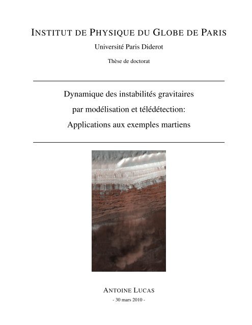
la son<strong>de</strong> Mars Reconnaissance Orbiter a fortuitem<strong>en</strong>t observé une avalanche au pôle Nord<br />
(photographie <strong>de</strong> couverture <strong>du</strong> manuscrit). Par ailleurs, <strong>de</strong> nouveaux slope streaks ont été observées
12 CHAPITRE 1. INTRODUCTION<br />
FIG. 1.10: Ravines formées sur les versants d’une <strong>du</strong>ne dans le Cratère Russell (−54.2 o N, 12.93 o E). Ces<br />
ravines prés<strong>en</strong>t<strong>en</strong>t <strong>de</strong>s levées ainsi que <strong>de</strong>s oscillations dont l’origine est discutée. (Image HiRISE).<br />
FIG. 1.11: Écoulem<strong>en</strong>ts fins (appelés « slope streaks ») observés ici sur le versant Nord d’Olympus Mons<br />
(23.3 o N, 223.7 o E), le plus grand volcan connu à ce jour. (Image HiRISE).
1.4. OBJECTIFS 13<br />
<strong>en</strong>tre <strong>de</strong>ux clichés différ<strong>en</strong>ts datant <strong>de</strong> 1999 et 2001 [Aharonson et al., 2003]. Ces événem<strong>en</strong>ts font<br />
l’objet <strong>de</strong> débats quant à la prés<strong>en</strong>ce ou non d’une phase flui<strong>de</strong> [Hoffman, 2000 ; Musselwhite et<br />
al., 2001 ; Mellon and Phillips, 2001 ; Costard et al., 2002 ; Schorghofer et. al., 2002 ; Aharonson et<br />
al., 2003 ; Mangold et al., 2003 ; Christ<strong>en</strong>s<strong>en</strong> et al., 2003 ; Treiman, 2003 ; Ishii and Sasaki, 2004 ;<br />
Heldmann and Mellon, 2004 ; Gerstell et al., 2004 ; Shinbrot et al., 2004 ; Heldmann et al., 2005 ;<br />
Balme et al., 2006 ; Levy et al., 2009 ; Mangold et al., 2010].<br />
Certains écoulem<strong>en</strong>ts prés<strong>en</strong>t<strong>en</strong>t <strong>de</strong>s sinuosités sur <strong>de</strong>s topographies complexes, interprétées<br />
comme le résultat d’écoulem<strong>en</strong>t aqueux bi<strong>en</strong> que les conditions d’eau liqui<strong>de</strong> à la surface <strong>de</strong> Mars ne<br />
soi<strong>en</strong>t pas prés<strong>en</strong>tes actuellem<strong>en</strong>t [Heldman and Mellon, 2004]. Néanmoins, <strong>de</strong>s travaux ont montré<br />
que la glace d’eau était stable <strong>en</strong> profon<strong>de</strong>ur à haute latitu<strong>de</strong> [Feldman et al., 2004]. D’autres étu<strong>de</strong>s<br />
ont proposé que les fortes variations d’obliquité <strong>de</strong> la planète pouvai<strong>en</strong>t <strong>en</strong>traîner <strong>de</strong>s changem<strong>en</strong>ts<br />
importants dans la distribution géographique <strong>de</strong> cette glace d’eau au cours <strong>du</strong> temps [Mellon and Jakosky,<br />
1995]. Enfin, d’autres types d’écoulem<strong>en</strong>ts granulaires sont observés sur <strong>de</strong>s topographies à<br />
faible p<strong>en</strong>te (< 10 o ) et prés<strong>en</strong>t<strong>en</strong>t ainsi une gran<strong>de</strong> mobilité. Comme pour les grands glissem<strong>en</strong>ts, la<br />
prise <strong>en</strong> compte <strong>de</strong> la topographie sous-jac<strong>en</strong>te permet-elle d’expliquer les morphologies observées ?<br />
1.4 Objectifs<br />
Les observations <strong>de</strong> terrain montr<strong>en</strong>t une gran<strong>de</strong> mobilité <strong>de</strong>s écoulem<strong>en</strong>ts naturels sur Terre<br />
comme sur Mars. Malgré le nombre d’étu<strong>de</strong>s qui se réfèr<strong>en</strong>t à cette mobilité, il semble qu’il y ait<br />
<strong>de</strong>s problèmes liés à la définition <strong>de</strong>s paramètres pris <strong>en</strong> compte. Y a-t-il <strong>de</strong>s effets géométriques ou<br />
topographiques <strong>de</strong>rrière ce paramètre <strong>de</strong> mobilité ? Comm<strong>en</strong>t peut-on alors les quantifier ? En outre,<br />
peut-on vali<strong>de</strong>r le pouvoir prédictif <strong>de</strong>s modèles et retrouver <strong>de</strong>s informations sur les conditions<br />
initiales à partir <strong>du</strong> dépôt ? Enfin, quelle gamme <strong>de</strong> valeur obti<strong>en</strong>t t-on pour le paramètre <strong>de</strong> friction ?<br />
Peut-on conclure à l’implication d’une phase liqui<strong>de</strong> ?<br />
La modélisation numérique s’avère indisp<strong>en</strong>sable pour, d’une part, extrapoler les résultats expérim<strong>en</strong>taux<br />
(lois d’échelle) à l’échelle <strong>du</strong> terrain et, d’autre part, tester différ<strong>en</strong>tes conditions initiales<br />
(géométrie <strong>de</strong> la masse, volume, morphologie <strong>de</strong> la surface <strong>de</strong> rupture. . .) ainsi que les effets topographiques.
14 CHAPITRE 1. INTRODUCTION<br />
Le travail m<strong>en</strong>é ici se propose donc d’étudier à l’ai<strong>de</strong> <strong>du</strong> modèle numérique SHALT OP les<br />
interactions complexes <strong>en</strong>tre topographie et écoulem<strong>en</strong>t granulaire et d’appliquer les analyses aux<br />
cas marti<strong>en</strong>s et terrestres. En effet, ces exemples offr<strong>en</strong>t un cadre unique d’étu<strong>de</strong> à la fois grâce à la<br />
bonne conservation <strong>de</strong>s dépôts et à la disponibilité <strong>de</strong> nombreuses données haute résolution.<br />
Dans un premier temps, il convi<strong>en</strong>t <strong>de</strong> circonscrire le domaine <strong>de</strong> validité <strong>du</strong> modèle numérique<br />
<strong>en</strong> le confrontant à <strong>de</strong>s expéri<strong>en</strong>ces <strong>en</strong> laboratoire et à <strong>de</strong>s cas naturels avec peu d’incertitu<strong>de</strong> sur le<br />
volume <strong>de</strong> la masse et sur la topographie <strong>du</strong> glissem<strong>en</strong>t.<br />
La dynamique repro<strong>du</strong>ite par la modélisation sera <strong>en</strong>suite confrontée à une analyse <strong>de</strong>s on<strong>de</strong>s<br />
sismiques générées par l’avalanche. Une confrontation avec <strong>de</strong>s données <strong>de</strong> terrain sera alors m<strong>en</strong>ée<br />
<strong>en</strong> partie 3.<br />
Les étu<strong>de</strong>s précéd<strong>en</strong>tes se bas<strong>en</strong>t généralem<strong>en</strong>t sur <strong>de</strong>s topographies planes ou inclinées. Nous<br />
nous proposons ici d’utiliser directem<strong>en</strong>t <strong>de</strong> vraies topographies. Cep<strong>en</strong>dant, la modélisation numérique<br />
d’avalanche <strong>de</strong> roche <strong>de</strong>man<strong>de</strong> <strong>de</strong> connaître la topographie sous-jac<strong>en</strong>te. Ceci implique, pour<br />
les cas marti<strong>en</strong>s <strong>en</strong> particulier, <strong>de</strong> reconstruire cette topographie. Le développem<strong>en</strong>t d’un tel procédé<br />
<strong>de</strong>man<strong>de</strong> <strong>en</strong> amont <strong>de</strong> maîtriser le traitem<strong>en</strong>t <strong>de</strong>s données (imagerie et topographie) acquises<br />
par les missions spatiales. Après avoir décrit la nature et le traitem<strong>en</strong>t <strong>de</strong> ces données, une métho<strong>de</strong><br />
d’extraction <strong>de</strong> topographie à haute résolution à partir <strong>de</strong> paires d’images par stéréoscopie sera prés<strong>en</strong>tée.<br />
Puis, la métho<strong>de</strong> <strong>de</strong> reconstrution topographique pour les glissem<strong>en</strong>ts <strong>de</strong> terrain marti<strong>en</strong>s sera<br />
détaillée.<br />
À l’ai<strong>de</strong> <strong>de</strong>s outils préalablem<strong>en</strong>t décrits, une analyse <strong>de</strong>s effets topographiques sur la morphologie<br />
<strong>de</strong>s dépôts d’écoulem<strong>en</strong>t granulaire sera m<strong>en</strong>ée afin d’<strong>en</strong> étudier les implications concernant<br />
les sinuosités observées sur les ravines marti<strong>en</strong>nes.<br />
Depuis une analyse dim<strong>en</strong>sionnelle, nous verrons qu’il est possible <strong>de</strong> détacher les effets topographiques<br />
<strong>de</strong>s effets géométriques dans la paramétrisation <strong>de</strong> la mobilité. Ce paramètre servira par<br />
la suite pour la calibration <strong>de</strong>s modèles.<br />
Enfin, <strong>de</strong>s expéri<strong>en</strong>ces numériques m<strong>en</strong>ées sur la géométrie <strong>de</strong> l’escarpem<strong>en</strong>t <strong>de</strong>s glissem<strong>en</strong>ts <strong>de</strong><br />
terrain seront détaillées. L’application directe sur <strong>de</strong>s modèles numériques <strong>de</strong> terrain reconstruits à<br />
partir <strong>de</strong>s métho<strong>de</strong>s décrites <strong>en</strong> partie 4 permettra <strong>de</strong> vali<strong>de</strong>r les tests théoriques. Nous <strong>en</strong> verrons les<br />
effets et les implications géologiques pour les glissem<strong>en</strong>ts <strong>de</strong> terrain marti<strong>en</strong>s.
Chapitre 2<br />
Modélisation numérique d’avalanches<br />
granulaires<br />
2.1 Description <strong>du</strong> modèle<br />
La modélisation physique <strong>de</strong>s écoulem<strong>en</strong>ts gravitaires est motivée par le risque que ces événem<strong>en</strong>ts<br />
in<strong>du</strong>is<strong>en</strong>t pour les populations dans les régions volcaniques et montagneuses <strong>en</strong> particulier. En<br />
outre, le contexte sci<strong>en</strong>tifique qu’offre ce type <strong>de</strong> processus concerne un large spectre disciplinaire,<br />
aussi bi<strong>en</strong> <strong>en</strong> mécanique, <strong>en</strong> géophysique qu’<strong>en</strong> géomorphologie.<br />
La compréh<strong>en</strong>sion physique <strong>de</strong> ces événem<strong>en</strong>ts <strong>de</strong>man<strong>de</strong> d’étudier les processus <strong>de</strong> décl<strong>en</strong>chem<strong>en</strong>t<br />
d’une part et la phase <strong>de</strong> propagation d’autre part. C’est cette secon<strong>de</strong> phase qui nous intéresse<br />
ici. Actuellem<strong>en</strong>t, la <strong>de</strong>scription physique <strong>de</strong> la propagation se heurte à l’abs<strong>en</strong>ce <strong>de</strong> loi <strong>de</strong> comportem<strong>en</strong>t<br />
correctem<strong>en</strong>t établie.<br />
L’approche empruntée est <strong>de</strong> tester, à l’ai<strong>de</strong> d’un modèle numérique, les lois <strong>de</strong> comportem<strong>en</strong>t<br />
et d’<strong>en</strong> évaluer les effets sur la dynamique et sur la morphologie <strong>de</strong>s dépôts. La mise au point <strong>de</strong><br />
modèles physiques implique nécessairem<strong>en</strong>t <strong>de</strong>s hypothèses, à la fois sur le comportem<strong>en</strong>t et sur<br />
le matériau lui-même, <strong>en</strong> particulier pour <strong>de</strong>s effondrem<strong>en</strong>ts naturels dont la nature (composition,<br />
granulométrie, structure. . .) n’est pas connue. Et même si la nature <strong>du</strong> matériau est connue, la <strong>de</strong>scription<br />
physique n’<strong>en</strong> est pas simple. En outre, la prise <strong>en</strong> compte <strong>de</strong> tous les processus connus pose<br />
<strong>de</strong>s problèmes <strong>de</strong> temps <strong>de</strong> calcul.<br />
17
18 CHAPITRE 2. MODÉLISATION NUMÉRIQUE D’AVALANCHES GRANULAIRES<br />
Deux approches basées sur <strong>de</strong>s concepts physiques coexist<strong>en</strong>t à l’heure actuelle : l’approche dite<br />
"granulaire" ou discrète et l’approche "hydrodynamique". Si la philosophie <strong>de</strong> ces <strong>de</strong>ux approches<br />
est radicalem<strong>en</strong>t différ<strong>en</strong>te, elles s’attach<strong>en</strong>t néanmoins toutes <strong>de</strong>ux à décrire le comportem<strong>en</strong>t d’une<br />
masse <strong>en</strong> mouvem<strong>en</strong>t sous l’influ<strong>en</strong>ce <strong>de</strong> la gravité. C’est l’aptitu<strong>de</strong> <strong>de</strong>s matériaux granulaires à se<br />
comporter parfois comme un soli<strong>de</strong>, parfois comme un liqui<strong>de</strong> et d’<strong>en</strong> décrire alors la transition qui<br />
justifie le nombre d’approches théoriques existantes aujourd’hui.<br />
Le modèle SHALT OP utilisé dans cette étu<strong>de</strong> est le fruit d’une collaboration étroite <strong>en</strong>tre l’<strong>Institut</strong><br />
<strong>de</strong> <strong>Physique</strong> <strong>du</strong> <strong>Globe</strong> <strong>de</strong> <strong>Paris</strong> et le Départem<strong>en</strong>t <strong>de</strong> Mathématiques Appliquées <strong>de</strong> l’École Normale<br />
Supérieure <strong>de</strong> <strong>Paris</strong>. Il décrit l’effondrem<strong>en</strong>t d’une masse granulaire s’écoulant sur une topographie<br />
complexe quelconque [Bouchut et al., 2003 ; Bouchut and Westdick<strong>en</strong>berg, 2004 ; Mang<strong>en</strong>ey-<br />
Castelnau et al., 2005, Mang<strong>en</strong>ey et al., 2007a]. Le modèle est basé sur l’approximation d’on<strong>de</strong><br />
longue se basant sur l’hypothèse que l’épaisseur <strong>de</strong> l’écoulem<strong>en</strong>t est significativem<strong>en</strong>t plus petite<br />
que la longueur <strong>de</strong> celui-ci. Il pr<strong>en</strong>d <strong>en</strong> compte une friction <strong>de</strong> type Coulomb suivant les travaux<br />
<strong>de</strong> Savage and Hutter [1989] et décrit l’évolution temporelle <strong>de</strong> l’épaisseur h(x, y) et <strong>de</strong> la vitesse<br />
intégrée <strong>de</strong> l’écoulem<strong>en</strong>t u(x, y) le long d’une topographie quelconque.<br />
À l’inverse <strong>de</strong> l’approche classique (Hutter et collaborateurs), les équations dans le modèle<br />
SHALT OP sont exprimées dans le repère cartési<strong>en</strong> (x, y, z), alors que l’approximation d’on<strong>de</strong><br />
longue est effectuée dans le repère lié à la topographie (X, Y, Z) (Figure 2.1). Ainsi, l’accélération<br />
normale à la topographie est négligée par rapport au gradi<strong>en</strong>t <strong>de</strong> pression normale à la topographie.<br />
L’analyse asymptotique rigoureuse 1 permet ainsi la prise <strong>en</strong> compte <strong>de</strong> la matrice <strong>de</strong> courbure <strong>de</strong> la<br />
topographie H définie par<br />
⎛<br />
⎞<br />
1<br />
H = ⎝√<br />
⎠<br />
1 + ||∇ x b|| 2<br />
3<br />
·<br />
⎛<br />
⎜<br />
⎝<br />
∂ 2 b<br />
∂x 2<br />
∂ 2 b<br />
∂x∂y<br />
∂ 2 b<br />
∂x∂y<br />
∂ 2 b<br />
∂ 2 b<br />
⎞<br />
⎟<br />
⎠ , (2.1.1)<br />
où la fonction scalaire b(x, y) décrit la topographie 3D, ∇ x est le vecteur gradi<strong>en</strong>t dans le plan<br />
horizontal x, y et le vecteur 2D x = (x, y) ∈ R 2 décrit les coordonnées dans le repère horizontal. Le<br />
1 Somme finie <strong>de</strong> fonctions <strong>de</strong> référ<strong>en</strong>ce donnant une approximation d’une fonction donnée plus complexe afin d’<strong>en</strong><br />
décrire le comportem<strong>en</strong>t au voisinage considéré.
2.1. DESCRIPTION DU MODÈLE 19<br />
vecteur unitaire 3D normal à la topographie est défini par<br />
⃗n ≡ (−s, c) ∈ R 2 × R, avec s =<br />
∇ x b<br />
√<br />
1 + ||∇ x b|| , et c = 1<br />
√1 2 + ||∇ x b|| , (2.1.2)<br />
2<br />
où c = cos θ, avec θ définissant l’angle <strong>en</strong>tre la normale à la topographie ⃗n et la verticale. Les<br />
vecteurs 3D sont notés avec une flèche⃗· et les vecteurs 2D sont notés <strong>en</strong> gras. Ainsi, l’écoulem<strong>en</strong>t<br />
est décrit par<br />
h(t, x) ≥ 0, u ′ (t, x) ∈ R 2 , (2.1.3)<br />
où h est l’épaisseur dans la direction normale à la topographie, et u ′ = (u, u t ) (avec l’indice t<br />
pour transverse) est une paramétrisation <strong>de</strong> la vitesse. La vitesse réelle 3D dans le repère cartési<strong>en</strong><br />
peut être dé<strong>du</strong>ite <strong>de</strong> cette paramétrisation <strong>de</strong> la vitesse et s’écrit<br />
−→ u = (cu ′ , s · u ′ ) . (2.1.4)<br />
Cette vitesse physique est tang<strong>en</strong>te à la topographie −→ u · −→ n = 0 et peut être exprimée comme<br />
vecteur 2D u = (u, v) dans le repère (X,Y ). À 1D, u ′ décrit alors la vitesse tang<strong>en</strong>te à la topographie.<br />
FIG. 2.1: Référ<strong>en</strong>tiel et variables utilisées dans le modèle, avec h l’épaisseur, u la vitesse, R x le rayon <strong>de</strong><br />
courbure, (X, Y, Z) le repère lié à la topographie et (x, y, z) le repère cartési<strong>en</strong>. Figure d’après Mang<strong>en</strong>ey et<br />
al., [2007a].<br />
Dans le cas d’un écoulem<strong>en</strong>t sur plan incliné dans la direction x, la vitesse réelle est décrite dans<br />
le repère (X, Y ) et a pour composantes u = (u, v) = (u, cu t ). Dans le repère horizontal, le modèle
20 CHAPITRE 2. MODÉLISATION NUMÉRIQUE D’AVALANCHES GRANULAIRES<br />
se formule<br />
∂ t (h/c) + ∇ x · (hu ′ ) = 0, (2.1.5)<br />
∂ t u ′ + cu ′ · ∇ x u ′ + 1 (Id − c sst ) ∇ x (g (hc + b)) =<br />
(<br />
− 1 c u ′t Hu ′) ( )<br />
s + 1 c (st Hu ′ ) u ′ gµcu<br />
− √<br />
′<br />
1 +<br />
u ′t Hu ′<br />
c 2 ‖u ′ ‖ 2 +(s·u ′ ) 2 gc<br />
+<br />
(2.1.6)<br />
où g est l’accélération <strong>de</strong> la gravité et µ le coeffici<strong>en</strong>t <strong>de</strong> friction. L’indice + indique la partie<br />
positive <strong>de</strong> l’expression x + = max(0, x). Dans le cas d’un écoulem<strong>en</strong>t sur plan incliné dans la<br />
direction x, les équations se ré<strong>du</strong>is<strong>en</strong>t à<br />
∂h<br />
∂t + c∂(hu) ∂x<br />
+ ∂(hv)<br />
∂y<br />
= 0, (2.1.7)<br />
∂u<br />
∂t + cu∂u ∂x + v ∂u<br />
∂y + c∂(ghc) ∂x<br />
= −g sin θ + f x , (2.1.8)<br />
∂v<br />
∂t + cu∂v ∂x + v ∂v<br />
∂y + ∂(ghc)<br />
∂y<br />
= f y (2.1.9)<br />
où f = (f x , f y ) décrit la force <strong>de</strong> friction parallèle à la topographie. Les coordonnées notées<br />
X sont définies par X = x/c, c∂/∂x = ∂/∂X et (2.1.7)-(2.1.9) peuv<strong>en</strong>t ainsi être ré<strong>du</strong>ites aux<br />
équations classiques <strong>de</strong> Savage and Hutter, [1989].<br />
La transition <strong>en</strong>tre l’état statique (pour lequel u = 0) et l’état dynamique (où u ≠ 0) est modélisée<br />
par l’intro<strong>du</strong>ction d’un seuil <strong>de</strong> Coulomb σ c . La mise <strong>en</strong> mouvem<strong>en</strong>t est alors possible lorsque<br />
la force motrice ‖f‖ <strong>de</strong>vi<strong>en</strong>t plus élevée que ce seuil σ c [Mang<strong>en</strong>ey-Castelnau et al., 2003]. Dans le<br />
modèle (2.1.8)-(2.1.9), f est exprimée par<br />
‖f‖ ≥ σ c ⇒ f = −gcµ u<br />
‖u‖ , (2.1.10)<br />
‖f‖ < σ c ⇒ u = 0,<br />
où σ c = gcµ, avec µ = tan δ le coeffici<strong>en</strong>t <strong>de</strong> friction (et δ l’angle <strong>de</strong> friction). Lorsque le<br />
matériau dépasse le seuil σ c , la loi <strong>de</strong> Coulomb implique que la force <strong>de</strong> friction ait une direction<br />
opposée au champ <strong>de</strong> vitesse tang<strong>en</strong>tielle moy<strong>en</strong>né et l’amplitu<strong>de</strong> <strong>de</strong> cette force <strong>de</strong> friction est alors<br />
proportionnelle à la contrainte normale et au coeffici<strong>en</strong>t <strong>de</strong> friction µ.
2.1. DESCRIPTION DU MODÈLE 21<br />
L’avalanche <strong>de</strong> débris est donc traitée ici comme un matériau monophasique, sec, <strong>de</strong> type coulombi<strong>en</strong>.<br />
Le coeffici<strong>en</strong>t <strong>de</strong> friction µ est alors supposé être<br />
1. constant dans le cas <strong>de</strong> la loi <strong>de</strong> Coulomb :<br />
µ = tan δ, (2.1.11)<br />
où δ est l’angle <strong>de</strong> friction constant, ou<br />
2. dép<strong>en</strong>dant <strong>de</strong> l’épaisseur h <strong>de</strong> l’écoulem<strong>en</strong>t et <strong>du</strong> nombre <strong>de</strong> Frou<strong>de</strong> F r = ||u||/ √ gh, où<br />
||u|| est la norme <strong>de</strong> la vitesse moy<strong>en</strong>née <strong>de</strong> l’écoulem<strong>en</strong>t, dans le cas <strong>de</strong> la loi <strong>de</strong> Pouliqu<strong>en</strong><br />
[Pouliqu<strong>en</strong> et al., 1999] :<br />
– Si F r > β<br />
– Si F r = 0<br />
1<br />
µ(h, F r) = tan δ 1 + (tan δ 2 − tan δ 1 )<br />
βh<br />
(2.1.12)<br />
+ 1.<br />
F rL<br />
µ(h, F r) = tan δ 3 + (tan δ 4 − tan δ 3 )<br />
h<br />
L<br />
1<br />
(2.1.13)<br />
+ 1.<br />
où δ i , i = 1, 4 sont les angles <strong>de</strong> friction caractéristiques <strong>du</strong> matériau, L est une longueur<br />
caractéristique dé<strong>du</strong>ite <strong>de</strong>s expéri<strong>en</strong>ces <strong>en</strong> laboratoire et β = 0.136 un paramètre sans dim<strong>en</strong>sion<br />
proposé par Pouliqu<strong>en</strong>, [1999] pour les billes <strong>de</strong> verre. Ainsi, la friction augm<strong>en</strong>te lorsque<br />
l’épaisseur h est faible et la vitesse u est gran<strong>de</strong>.<br />
La loi <strong>de</strong> Pouliqu<strong>en</strong> a permis <strong>de</strong> repro<strong>du</strong>ire <strong>de</strong>s expéri<strong>en</strong>ces d’effondrem<strong>en</strong>ts granulaires [Mang<strong>en</strong>ey-<br />
Castelnau et al., 2005] ainsi que <strong>de</strong> simuler les morphologies <strong>de</strong> type levées-ch<strong>en</strong>al observées sur<br />
le terrain [ Mang<strong>en</strong>ey et al., 2007a ; Mangold et al., 2010]. Néanmoins, le nombre important <strong>de</strong><br />
paramètres impliqués la r<strong>en</strong>d délicate à l’emploi et il n’est pas clair qu’elle apporte une réelle amélioration<br />
dans la simulation d’écoulem<strong>en</strong>ts géophysiques réels par rapport à la loi <strong>de</strong> Coulomb qui<br />
n’implique qu’un seul paramètre [Pirulli et al., 2007 ; ıPirulli and Mang<strong>en</strong>ey, 2008 ; ıKuo et al. ,<br />
2009, Lucas et al., 2010].<br />
La pertin<strong>en</strong>ce <strong>de</strong> l’approximation d’on<strong>de</strong> longue avec la loi <strong>de</strong> friction <strong>de</strong> type Coulomb a été<br />
testée <strong>en</strong> comparant le modèle SHALT OP à <strong>de</strong>s simulations par élém<strong>en</strong>ts discrets. Plusieurs simulations<br />
d’effondrem<strong>en</strong>ts <strong>de</strong> colonne ont été effectuées <strong>en</strong> changeant le rapport d’aspect initial<br />
(a = H i /L i , où H i et L i sont respectivem<strong>en</strong>t l’épaisseur et la longueur initiales <strong>de</strong> la masse) [Mang<strong>en</strong>ey<br />
et al., 2006]. Les résultats ont montré que le modèle intégré ne donnait pas <strong>de</strong> bons résultats
22 CHAPITRE 2. MODÉLISATION NUMÉRIQUE D’AVALANCHES GRANULAIRES<br />
pour <strong>de</strong>s rapports d’aspects a > 1. Dans ce cas, l’accélération verticale doit être prise <strong>en</strong> compte<br />
dans le modèle. Néanmoins, pour la majorité <strong>de</strong>s cas naturels, le rapport d’aspect est inférieur à 1,<br />
permettant ainsi l’utilisation <strong>de</strong>s modèles <strong>de</strong> couche mince.<br />
2.2 Évolution <strong>du</strong> co<strong>de</strong> pour une utilisation <strong>en</strong> géophysique<br />
Les dim<strong>en</strong>sions <strong>de</strong>s exemples naturels ont <strong>de</strong>mandé la parallélisation <strong>du</strong> modèle initial sous<br />
instructions MPI 2 . La parallélisation <strong>du</strong> co<strong>de</strong> a été effectuée par Patrick Stoclet, alors ingénieur <strong>en</strong><br />
calculs parallèles à l’IPGP <strong>en</strong> 2007. Cette évolution se tra<strong>du</strong>it par un découpage <strong>de</strong> la grille d’espace<br />
<strong>en</strong> sous-domaines distribués à chaque unité <strong>de</strong> calcul 3 . Le travail prés<strong>en</strong>té dans cette thèse correspond<br />
aux premières utilisations <strong>de</strong> cette version. La validation <strong>de</strong> cette nouvelle version <strong>du</strong> co<strong>de</strong> (nommée<br />
SHALT OP mpi ) a été effectuée <strong>en</strong> partie par P. Stoclet et <strong>en</strong> partie dans le cadre <strong>de</strong> ce travail par<br />
comparaison avec la version séqu<strong>en</strong>tielle (SEQ).<br />
Les différ<strong>en</strong>ces observées <strong>en</strong>tre les <strong>de</strong>ux versions sont illustrées ici à travers <strong>de</strong>s exemples <strong>de</strong><br />
simulations réalisées <strong>de</strong>puis un profil topographique 2D issu <strong>du</strong> MNT 4 <strong>de</strong> l’avalanche <strong>de</strong> Punta<br />
Thurwieser <strong>du</strong> 18 septembre 2004 <strong>en</strong> Italie (Figure 2.2). La grille utilisée est constituée <strong>de</strong> 324 × 50<br />
points <strong>de</strong> calcul avec <strong>de</strong>s pas d’espace ∆x = 10 m et ∆y = 2 m. Le temps complet <strong>de</strong> simulation<br />
est <strong>de</strong> 100 secon<strong>de</strong>s.<br />
Dans le modèle SHALT OP , le pas <strong>en</strong> temps est contrôlé par une condition <strong>de</strong> type CFL 5 qui est<br />
une fonction <strong>de</strong> la vitesse, <strong>du</strong> pas <strong>de</strong> temps et <strong>du</strong> pas d’espace. Ainsi, pour un pas d’espace donné,<br />
plus la vitesse est gran<strong>de</strong> et plus petit sera le pas <strong>de</strong> temps. Ceci permet d’obt<strong>en</strong>ir une meilleure<br />
<strong>de</strong>scription <strong>de</strong> l’écoulem<strong>en</strong>t lorsque les gradi<strong>en</strong>ts sont grands. Ainsi, les temps <strong>de</strong> sortie dép<strong>en</strong>d<strong>en</strong>t<br />
<strong>de</strong>s gradi<strong>en</strong>ts calculés au cours <strong>du</strong> temps. Les temps <strong>de</strong> sortie sont strictem<strong>en</strong>t les mêmes <strong>en</strong>tre<br />
séqu<strong>en</strong>tiel et MPI jusqu’à l’incrém<strong>en</strong>t 40 soit t = 78s. L’écart maximal <strong>en</strong>tre séqu<strong>en</strong>tiel et MPI est<br />
<strong>de</strong> 0.0115s pour un ∆t = 0.036s (Figure 2.3). La différ<strong>en</strong>ce <strong>en</strong>tre les <strong>de</strong>ux versions est inférieure<br />
au pas <strong>de</strong> temps ∆t. Ces très faibles différ<strong>en</strong>ces à la fin <strong>de</strong> la simulation s’expliqu<strong>en</strong>t si l’on regar<strong>de</strong><br />
2 Message Passing Interface : standard <strong>de</strong> communication pour <strong>de</strong>s nœuds exécutant <strong>de</strong>s programmes parallèles sur<br />
<strong>de</strong>s systèmes à mémoire distribuée comme un cluster.<br />
3 L’arrivée <strong>de</strong> processeurs à plusieurs noyaux amène à considérer un noyau comme unité <strong>de</strong> calcul et non le processeur.<br />
Dans le cas <strong>du</strong> service <strong>de</strong> calcul parallèle et <strong>de</strong> traitem<strong>en</strong>t <strong>de</strong> données <strong>en</strong> sci<strong>en</strong>ces <strong>de</strong> la Terre (S-CAPAD) <strong>de</strong> l’IPGP, la<br />
grille <strong>de</strong> calcul utilise <strong>de</strong>s nœuds cont<strong>en</strong>ant <strong>de</strong>ux processeurs quad-core soit huit unités <strong>de</strong> calcul par nœud.<br />
4 Modèle Numérique <strong>de</strong> Terrain issu <strong>de</strong>s données SRTM.<br />
5 Courant-Friedrichs-Levy
2.2. ÉVOLUTION DU CODE POUR UNE UTILISATION EN GÉOPHYSIQUE 23<br />
FIG. 2.2: Évolution <strong>de</strong> la masse (<strong>en</strong> rouge) le long <strong>du</strong> profil topographique (<strong>en</strong> noir) au cours <strong>du</strong> temps.<br />
l’épaisseur et la vitesse <strong>de</strong> l’écoulem<strong>en</strong>t dans les <strong>de</strong>ux simulations. La comparaison <strong>de</strong> l’évolution <strong>de</strong><br />
l’épaisseur h(x, y, t) au c ours <strong>du</strong> temps montre un excell<strong>en</strong>t accord <strong>en</strong>tre les <strong>de</strong>ux versions <strong>du</strong> co<strong>de</strong><br />
et, ce, pour l’<strong>en</strong>semble <strong>de</strong>s sorties <strong>en</strong> temps disponibles (Figure 2.4). À l’inverse, l’évolution <strong>de</strong> la<br />
composante x <strong>de</strong> la vitesse u au cours <strong>du</strong> temps diffère <strong>du</strong> co<strong>de</strong> SEQ au co<strong>de</strong> MPI à t = 68s (Figure<br />
2.5). Il s’agit <strong>de</strong> régions pour lesquelles l’épaisseur h est nulle ou très petite <strong>de</strong>vant 1. Le caractère<br />
continu <strong>du</strong> modèle <strong>en</strong>traîne <strong>de</strong> fortes vitesses pour un h très petit. Ce sont dans ces régions que les<br />
différ<strong>en</strong>ces <strong>en</strong>tre le co<strong>de</strong> SEQ et le co<strong>de</strong> MPI sont observées. Si la vitesse u est filtrée par rapport à<br />
l’épaisseur h pour h < d avec d = 0.01, 0.5m, un excell<strong>en</strong>t accord <strong>en</strong>tre les <strong>de</strong>ux versions <strong>du</strong> co<strong>de</strong><br />
est alors obt<strong>en</strong>u (Figures 2.6,2.7 et 2.8). Les différ<strong>en</strong>ces observées sont liées à la nature continue <strong>du</strong><br />
modèle qui nécessite d’imposer une épaisseur minimale qui pourra varier <strong>en</strong> fonction <strong>du</strong> cas d’étu<strong>de</strong>.
24 CHAPITRE 2. MODÉLISATION NUMÉRIQUE D’AVALANCHES GRANULAIRES<br />
De plus, les précisions <strong>de</strong>s machines utilisées (station et cluster) peuv<strong>en</strong>t <strong>en</strong>traîner <strong>de</strong> très légères<br />
différ<strong>en</strong>ces.<br />
FIG. 2.3: (<strong>en</strong> haut) Temps physique pour chaque itération <strong>de</strong> sortie <strong>de</strong> fichiers pour les <strong>de</strong>ux versions <strong>du</strong> co<strong>de</strong>.<br />
(<strong>en</strong> bas) Différ<strong>en</strong>ce <strong>en</strong>tre ces <strong>de</strong>ux temps <strong>de</strong> sortie (t SEQ − t MP I ).<br />
Afin <strong>de</strong> quantifier l’efficacité <strong>de</strong> cette version MPI, une série <strong>de</strong> tests a été m<strong>en</strong>ée à partir d’un<br />
exemple simple : l’étalem<strong>en</strong>t <strong>de</strong> colonne sur un plan horizontal. La géometrie <strong>de</strong> la masse initiale<br />
est cylindrique avec un rapport d’aspect initial <strong>de</strong> 0.56, afin <strong>de</strong> respecter l’approximation d’on<strong>de</strong><br />
longue. Nous avons utilisé une grille <strong>de</strong> 1000x1000 points et un temps <strong>de</strong> simulation <strong>de</strong> 700ms avec<br />
les options <strong>de</strong> compilations suivantes :<br />
ifort : -i4 -assume byterecl -O2 -axS<br />
Les résultats illustrés par la figure 2.9 montr<strong>en</strong>t la bonne scalabilité <strong>du</strong> co<strong>de</strong> MPI jusqu’à un<br />
nombre d’unités <strong>de</strong> calcul égal à 48 lorsque le nombre <strong>de</strong> noyaux utilisés est égal à 4 par nœuds.<br />
Cette scalabilité est meilleure si la totalité <strong>de</strong>s unités <strong>de</strong> calcul par nœud est alors utilisée (ici 8).<br />
En définitive, le modèle MPI donne <strong>de</strong>s résultats très proches <strong>de</strong> ceux <strong>de</strong> la version séqu<strong>en</strong>tielle.<br />
Les différ<strong>en</strong>ces sont majoritairem<strong>en</strong>t observées pour <strong>de</strong>s épaisseur h très petite pour lesquelles la<br />
vitesse est gran<strong>de</strong>. Ceci ne pose donc pas problème pour la modélisation d’écoulem<strong>en</strong>ts naturels.
2.2. ÉVOLUTION DU CODE POUR UNE UTILISATION EN GÉOPHYSIQUE 25<br />
FIG. 2.4: Évolution <strong>de</strong> l’épaisseur <strong>de</strong> la masse au cours <strong>du</strong> temps pour les <strong>de</strong>ux versions <strong>du</strong> co<strong>de</strong>.<br />
FIG. 2.5: Évolution <strong>de</strong> la composante x <strong>de</strong> la vitesse au cours <strong>du</strong> temps pour les <strong>de</strong>ux versions <strong>du</strong> co<strong>de</strong>.<br />
En outre, la version MPI montre une bonne scalabilité <strong>en</strong> particulier si l’<strong>en</strong>semble <strong>de</strong>s CPU d’un<br />
même nœud est utilisé. Cette version <strong>du</strong> co<strong>de</strong> sous instructions MPI va permettre l’étu<strong>de</strong> <strong>de</strong> cas
26 CHAPITRE 2. MODÉLISATION NUMÉRIQUE D’AVALANCHES GRANULAIRES<br />
FIG. 2.6: Évolution <strong>de</strong> la composante x <strong>de</strong> la vitesse filtrée pour h > 0.01m au cours <strong>du</strong> temps pour les <strong>de</strong>ux<br />
versions <strong>du</strong> co<strong>de</strong>.<br />
FIG. 2.7: Évolution <strong>de</strong> la composante x <strong>de</strong> la vitesse filtrée pour h > 0.5m au cours <strong>du</strong> temps pour les <strong>de</strong>ux<br />
versions <strong>du</strong> co<strong>de</strong>.<br />
géophysiques qui <strong>de</strong>mand<strong>en</strong>t <strong>de</strong> gran<strong>de</strong>s grilles <strong>de</strong> calcul (> 10 6 nœuds) et une quantité <strong>de</strong> mémoire<br />
trop importante pour la version séqu<strong>en</strong>tielle (> 4 Go).
2.2. ÉVOLUTION DU CODE POUR UNE UTILISATION EN GÉOPHYSIQUE 27<br />
FIG. 2.8: Différ<strong>en</strong>ce <strong>en</strong>tre les <strong>de</strong>ux modèles <strong>de</strong>s profils <strong>de</strong> vitesse aux temps t = 28, 68 et 100s pour différ<strong>en</strong>ts<br />
filtrages sur h.<br />
FIG. 2.9: Résultats <strong>de</strong>s tests <strong>de</strong> la version MPI <strong>du</strong> co<strong>de</strong>. À gauche est représ<strong>en</strong>té le temps <strong>de</strong> calcul <strong>en</strong> fonction<br />
<strong>du</strong> nombre d’unités <strong>de</strong> calcul. À droite est représ<strong>en</strong>tée l’efficacité <strong>du</strong> calcul <strong>en</strong> fonction <strong>du</strong> nombre d’unités <strong>de</strong><br />
calcul.<br />
2.2.1 Assimilation <strong>de</strong>s données<br />
L’approximation d’on<strong>de</strong> longue est effectuée dans le repère normal à la topographie (X, Y ) (voir<br />
section 2.1), ainsi l’épaisseur <strong>de</strong> l’écoulem<strong>en</strong>t est elle-même décrite selon la normale à la topographie<br />
sous-jac<strong>en</strong>te. Ceci ne pose pas <strong>de</strong> problème pour <strong>de</strong>s expéri<strong>en</strong>ces numériques simples, comme<br />
l’étalem<strong>en</strong>t <strong>de</strong> colonne sur un plan horizontal ou pour les écoulem<strong>en</strong>ts auto-ch<strong>en</strong>alisants sur plan in-
28 CHAPITRE 2. MODÉLISATION NUMÉRIQUE D’AVALANCHES GRANULAIRES<br />
cliné. En revanche, la simulation <strong>de</strong> cas naturels <strong>de</strong>man<strong>de</strong> un changem<strong>en</strong>t <strong>de</strong> repère car les données<br />
décrivant la masse à modéliser sont décrites initialem<strong>en</strong>t dans un repère cartési<strong>en</strong> (x, y).<br />
Si b x est le champ scalaire topographique dans le repère (x, y) et h X le champ scalaire <strong>de</strong> la<br />
masse dans le repère (X, Y ), alors le champ scalaire Hz x <strong>de</strong> la hauteur totale (masse + topographie)<br />
s’obti<strong>en</strong>t par :<br />
avec<br />
Hz x (x ′ , y ′ ) = b(x, y) + h(x, y) × c(x, y), (2.2.1)<br />
x ′ = x − s x (x, y) × h(x, y) × c(x, y), (2.2.2)<br />
et<br />
y ′ = x − s y (x, y) × h(x, y) × c(x, y), (2.2.3)<br />
où x ′ et y ′ sont les coordonnées cartési<strong>en</strong>nes <strong>du</strong> champ scalaire Hz x , s i sont les composantes x et<br />
y <strong>du</strong> gradi<strong>en</strong>t <strong>de</strong> la topographie et c = cos θ. Ainsi, Hz x est décrit dans un repère cartési<strong>en</strong> non<br />
régulier.<br />
FIG. 2.10: La surface marron représ<strong>en</strong>te la topographie sous-jac<strong>en</strong>te à la masse, représ<strong>en</strong>tée par la surface<br />
bleue transpar<strong>en</strong>te. Le champ normal à la topographie est représ<strong>en</strong>té par les vecteurs <strong>en</strong> rouges.<br />
Si ce changem<strong>en</strong>t <strong>de</strong> repère est simple dans le s<strong>en</strong>s (X, Y ) → (x, y) (équations (2.2.1)-(2.2.3)),<br />
il l’est beaucoup moins dans le s<strong>en</strong>s inverse qui nous intéresse ici. En effet, la surface qui décrit la<br />
masse n’est pas nécessairem<strong>en</strong>t parallèle à la surface topographique sous-jac<strong>en</strong>te (Figure 2.10).
2.3. CONFRONTATION DU MODÈLE 29<br />
Dans la plupart <strong>de</strong>s cas, la projection <strong>de</strong> H sur la normale à la topographie permet d’obt<strong>en</strong>ir une<br />
valeur approchée <strong>de</strong> l’épaisseur dans le repère topographique.<br />
2.3 Confrontation <strong>du</strong> modèle<br />
Dans le cadre <strong>de</strong> l’IFDLM 2007 (the 2007 International Forum on Landsli<strong>de</strong> Disaster Managem<strong>en</strong>t,<br />
Hong-Kong), nous avons bénéficié <strong>de</strong> données issues d’expéri<strong>en</strong>ces <strong>en</strong> laboratoire et<br />
d’exemples naturels étudiés à Hong Kong <strong>en</strong> particulier [Lucas et al., 2007]. L’objectif était <strong>de</strong><br />
déterminer les capacités et les limites <strong>de</strong> notre modèle numérique <strong>en</strong> terme <strong>de</strong> repro<strong>du</strong>ction et <strong>de</strong><br />
prédiction. Ces tests ont montré que dans presque tous les cas, le modèle que nous utilisons est<br />
capable <strong>de</strong> repro<strong>du</strong>ire les observations à l’échelle <strong>du</strong> terrain.<br />
2.3.1 Estimation <strong>de</strong> la dissipation numérique<br />
Mang<strong>en</strong>ey et al., [2000] ont proposé une solution analytique (SA) pour calibrer les modèles<br />
numériques d’effondrem<strong>en</strong>t granulaire et ainsi évaluer la dissipation numérique. Ce test décrit la<br />
position <strong>du</strong> front h(x, t) d’une masse <strong>en</strong> écoulem<strong>en</strong>t sur une p<strong>en</strong>te topographique d’angle θ avec un<br />
angle <strong>de</strong> friction δ qui est défini par<br />
⎧<br />
⎪⎨<br />
h(x, t) =<br />
⎪⎩<br />
1<br />
9g cos θ<br />
H<br />
(<br />
2c0 − x t − mt<br />
2<br />
; x ≤ −x r<br />
) 2<br />
; −x r < x < x l<br />
0 ; x l ≤ x<br />
avec<br />
m = g(cos θ tan δ − sin θ), (2.3.1)<br />
c 0 =<br />
√<br />
gH cos θ, (2.3.2)<br />
x l = 2c 0 t − 1 2 mt2 , (2.3.3)<br />
x r = c 0 t + 1 2 mt2 , (2.3.4)
30 CHAPITRE 2. MODÉLISATION NUMÉRIQUE D’AVALANCHES GRANULAIRES<br />
où H est la hauteur initiale <strong>de</strong> la masse, g la gravité, θ l’angle <strong>de</strong> la p<strong>en</strong>te et δ l’angle <strong>de</strong> friction<br />
(Figure 2.11).<br />
FIG. 2.11: Conditions initiales <strong>du</strong> test analytique. H est la hauteur initiale <strong>de</strong> la masse, θ l’angle <strong>de</strong> la p<strong>en</strong>te et<br />
δ l’angle <strong>de</strong> friction à la base <strong>du</strong> banc.<br />
Une comparaison simple <strong>en</strong>tre solution analytique et solution numérique utilisant les paramètres<br />
suivants :<br />
– épaisseur initiale : H = 10m ,<br />
– angle <strong>de</strong> la p<strong>en</strong>te : θ = 30 o ,<br />
– angle <strong>de</strong> friction : δ = 25 o ,<br />
illustre la faible dissipation numérique <strong>du</strong> modèle utilisé (Figure 2.12).<br />
Plus réc<strong>en</strong>t, le modèle SHALT OP est basé sur un schéma numérique d’ordre 2 et montre ainsi<br />
un meilleur accord avec la solution analytique que le modèle RASH 3D [Mang<strong>en</strong>ey et al., 2003].<br />
Le nouveau modèle repro<strong>du</strong>it avec un écart moindre à la solution analytique le profil <strong>de</strong> hauteur<br />
au niveau <strong>du</strong> front <strong>de</strong> l’écoulem<strong>en</strong>t (fig. 2.13). La surestimation <strong>de</strong> la distance au front, pour un<br />
temps donné avec le modèle cinétique, est directem<strong>en</strong>t reliée à la dissipation numérique, résultat<br />
d’une estimation <strong>de</strong>s dérivées trop simpliste. Ainsi, la calibration <strong>de</strong> ce modèle, par ajustem<strong>en</strong>t <strong>de</strong><br />
la distance <strong>de</strong> parcours maximale <strong>de</strong> l’écoulem<strong>en</strong>t, <strong>de</strong>man<strong>de</strong> nécessairem<strong>en</strong>t un angle <strong>de</strong> friction<br />
supérieur (+2 o dans notre exemple). Ceci à donc pour effet d’ajouter une incertitu<strong>de</strong> à l’angle <strong>de</strong><br />
friction. Dans le cadre <strong>du</strong> forum IFDLM, le modèle SHALT OP s’est montré particulièrem<strong>en</strong>t<br />
efficace pour repro<strong>du</strong>ire la solution analytique.
2.3. CONFRONTATION DU MODÈLE 31<br />
En conséqu<strong>en</strong>ce, le modèle d’ordre 2 apporte une amélioration importante <strong>en</strong> permettant <strong>de</strong><br />
ré<strong>du</strong>ire les incertitu<strong>de</strong>s liées à la discrétisation <strong>de</strong>s équations et ainsi augm<strong>en</strong>ter la confiance sur les<br />
paramètres utilisés dans la modélisation.<br />
FIG. 2.12: Hauteur h <strong>de</strong> l’écoulem<strong>en</strong>t aux temps t = 10, 20, 30 s pour la solution analytique (AS <strong>en</strong> rouge)<br />
et numérique (NS <strong>en</strong> noir) pour un incrém<strong>en</strong>t spatial <strong>en</strong> x, ∆x = 1.2 m. La solution analytique est très bi<strong>en</strong><br />
repro<strong>du</strong>ite par la solution numérique attestant d’une très faible dissipation numérique <strong>du</strong> modèle SHALT OP .<br />
1<br />
Fluid thickness h<br />
0.8<br />
0.6<br />
0.4<br />
0.2<br />
0<br />
500 1000 1500 2000<br />
x in m<br />
FIG. 2.13: (<strong>en</strong> haut) – Comparaison <strong>en</strong>tre le modèle RASH 3D et la solution analytique (<strong>de</strong>puis Mang<strong>en</strong>ey et<br />
al., [2003]). (<strong>en</strong> bas) – Comparaison <strong>en</strong>tre le modèle SHALT OP et la solution analytique.
32 CHAPITRE 2. MODÉLISATION NUMÉRIQUE D’AVALANCHES GRANULAIRES<br />
2.3.2 Confrontation aux expéri<strong>en</strong>ces <strong>en</strong> laboratoire<br />
Le modèle utilisé dans cette étu<strong>de</strong> a déjà fait l’objet <strong>de</strong> comparaisons avec <strong>de</strong>s expéri<strong>en</strong>ces <strong>en</strong><br />
laboratoire. Dans le cadre <strong>de</strong> l’article Mang<strong>en</strong>ey et al., [2005], <strong>de</strong>s étalem<strong>en</strong>ts <strong>de</strong> colonnes granulaires<br />
<strong>en</strong> laboratoire ont servi <strong>de</strong> témoin pour évaluer le modèle. Les principaux résultats montr<strong>en</strong>t que la<br />
distance maximale L f <strong>de</strong>s dépôts est fonction <strong>du</strong> rapport d’aspect initial a = H i /L i , avec H i la<br />
hauteur initiale et L i le rayon initial <strong>de</strong> la colonne.<br />
FIG. 2.14: Comparaison <strong>en</strong>tre la simulation et une expéri<strong>en</strong>ce d’effondrem<strong>en</strong>t <strong>de</strong> colonne Mang<strong>en</strong>ey et al.,<br />
[2005]. La morphologie <strong>de</strong>s dépôts est ici correctem<strong>en</strong>t repro<strong>du</strong>ite par la simulation pour un rapport d’aspect<br />
a = 0.56.<br />
Les expéri<strong>en</strong>ces montr<strong>en</strong>t égalem<strong>en</strong>t que, pour un tas <strong>de</strong> sable sec, il existe <strong>de</strong>ux régimes contrôlés<br />
par ce rapport d’aspect. Si a < 1 , la distance <strong>de</strong> parcours est une fonction linéaire <strong>de</strong> a. Si<br />
a > 1, la distance <strong>de</strong> parcours est contôlée par une loi <strong>de</strong> puissance. Il semble que, dans ce second<br />
cas, l’accélération verticale domine la phase <strong>de</strong> déstabilisation, alors qu’elle est négligeable lorsque<br />
que le rapport d’aspect a est inférieur à 1. Le modèle numérique utilisé ne pr<strong>en</strong>d pas <strong>en</strong> compte<br />
cette accélération verticale considérée négligeable face au gradi<strong>en</strong>t <strong>de</strong> pression vertical. D’autre<br />
part, l’hypothèse <strong>de</strong> couche mince n’est plus vérifiée dans le cas d’un rapport d’aspect élevé. Il n’est<br />
donc pas surpr<strong>en</strong>ant que le modèle ne repro<strong>du</strong>ise pas correctem<strong>en</strong>t la dynamique <strong>de</strong> l’étalem<strong>en</strong>t <strong>de</strong><br />
colonne pour <strong>de</strong> grands rapports d’aspect (typiquem<strong>en</strong>t a >> 1). À l’inverse, lorsque celui-ci est<br />
petit (a < 1), la dynamique et la géométrie <strong>de</strong>s dépôts observées dans les expéri<strong>en</strong>ces so nt correctem<strong>en</strong>t<br />
repro<strong>du</strong>ites par le modèle (Figure 2.14). Il existe ainsi un domaine <strong>de</strong> validité <strong>du</strong> modèle au<br />
regard <strong>du</strong> rapport d’aspect initial. Heureusem<strong>en</strong>t, les exemples naturels se trouv<strong>en</strong>t, dans une très<br />
large proportion, dans ce domaine <strong>de</strong> validité.
2.3. CONFRONTATION DU MODÈLE 33<br />
Le Ch<strong>en</strong>al 3D d’après Iverson et al., [2004]<br />
Iverson et al., [2004] ont proposé une expéri<strong>en</strong>ce d’effondrem<strong>en</strong>t <strong>de</strong> grains <strong>de</strong> sable le long d’un<br />
ch<strong>en</strong>al irrégulier réalisée <strong>en</strong> laboratoire. Le modèle numérique <strong>de</strong> terrain, obt<strong>en</strong>u par scanner laser,<br />
a permis d’effectuer la comparaison avec la simulation numérique.<br />
L’expéri<strong>en</strong>ce modèle est constituée <strong>de</strong> trois parties : un réservoir <strong>en</strong> amont, le ch<strong>en</strong>al lui-même<br />
placé <strong>en</strong>tre 9,14 cm et 39,12 cm et un réceptacle <strong>en</strong> aval (figure 2.15).<br />
Les caractéristiques géométriques <strong>de</strong> cette topographie sont :<br />
– angle moy<strong>en</strong> <strong>de</strong> la p<strong>en</strong>te dans le ch<strong>en</strong>al : 31.6 o ,<br />
– largeur <strong>de</strong> l’ouverture <strong>du</strong> réservoir : 12 cm,<br />
– X distance <strong>de</strong> l’ouverture : 8.858 cm,<br />
– Localisation <strong>du</strong> revêtem<strong>en</strong>t d’urethane <strong>de</strong> x = 9.14 cm à x = 39.12 cm<br />
– le prisme triangulaire <strong>du</strong> réservoir s’ét<strong>en</strong>d sur la largeur totale <strong>du</strong> modèle et atteint une hauteur<br />
<strong>de</strong> 4,35 cm au niveau <strong>de</strong> l’ouverture. L’épaisseur maximale <strong>de</strong> la masse h 0 = 4, 35 cm.<br />
Un revêtem<strong>en</strong>t d’uréthane a été placé au niveau <strong>du</strong> ch<strong>en</strong>al et <strong>du</strong> formica a été utilisé pour le<br />
réservoir et le réceptacle. La friction basale n’est donc pas homogène sur l’<strong>en</strong>semble <strong>du</strong> domaine <strong>de</strong><br />
l’expéri<strong>en</strong>ce. Les angles <strong>de</strong> friction basale calculés dans l’expéri<strong>en</strong>ce sont <strong>de</strong> 23.45 o pour le formica<br />
et 19.85 o pour l’uréthane [Iverson et al., 2004].<br />
Un ajustem<strong>en</strong>t <strong>du</strong> modèle numérique a été effectué pour pr<strong>en</strong>dre <strong>en</strong> compte ces variations <strong>de</strong><br />
friction. Aussi, pour les besoins <strong>de</strong> la simulation, le modèle numérique <strong>de</strong> terrain a été interpolé avec<br />
un pas d’espace ∆x = ∆y = 1.10 −3 m soit une grille <strong>de</strong> 562 × 201 points.<br />
Plusieurs simulations ont été réalisées. Les meilleurs résultats ont été obt<strong>en</strong>us avec un angle<br />
<strong>de</strong> friction <strong>de</strong> 26 o pour le réservoir et le réceptacle et <strong>de</strong> 23 o pour le ch<strong>en</strong>al (figure 2.16). Comme<br />
pour l’effondrem<strong>en</strong>t <strong>de</strong> colonne, le modèle à besoin d’angles <strong>de</strong> friction plus élevés (+ 3 o ) que ceux<br />
mesurés <strong>en</strong> laboratoire pour obt<strong>en</strong>ir la bonne dynamique.<br />
Cep<strong>en</strong>dant, la masse est déposée jusqu’à la sortie <strong>du</strong> ch<strong>en</strong>al dans les expéri<strong>en</strong>ces, alors qu’elle<br />
ne s’y dépose pas dans la simulation (Figure 2.17-(9)), la hauteur maximale <strong>de</strong>s dépôts est bi<strong>en</strong><br />
repro<strong>du</strong>ite par le modèle (Figure 2.17-(10)).<br />
L’analyse <strong>du</strong> champ <strong>de</strong> vitesse au niveau <strong>du</strong> réservoir permet <strong>de</strong> compr<strong>en</strong>dre la dynamique et<br />
la forme <strong>de</strong>s dépôts <strong>en</strong> amont à la fin <strong>de</strong> l’expéri<strong>en</strong>ce (Figure 2.18). En particulier, on observe sans
34 CHAPITRE 2. MODÉLISATION NUMÉRIQUE D’AVALANCHES GRANULAIRES<br />
FIG. 2.15: Ch<strong>en</strong>al irrégulier expérim<strong>en</strong>tal. La masse (ici <strong>en</strong> couleur) est initialem<strong>en</strong>t placée dans un réservoir<br />
<strong>en</strong> amont <strong>du</strong> ch<strong>en</strong>al. Le réceptacle et le réservoir sont revêtus <strong>de</strong> formica. Le ch<strong>en</strong>al est réalisé <strong>en</strong> uréthane.<br />
surprise que la vitesse est très faible au niveau <strong>de</strong>s dièdres (coins <strong>de</strong>rrière le mur <strong>du</strong> réservoir).<br />
À l’inverse, la vitesse maximale est observée au c<strong>en</strong>tre <strong>de</strong> l’ouverture. La purge s’effectue donc<br />
axialem<strong>en</strong>t d’où la forme <strong>en</strong> "V" obt<strong>en</strong>ue dans l’expéri<strong>en</strong>ce et dans la simulation (Figures 2.17-(6,8)<br />
et 2.18). Très rapi<strong>de</strong>m<strong>en</strong>t (t = 0.7 s), la vitesse dans les <strong>de</strong>ux coins <strong>de</strong>vi<strong>en</strong>t nulle. Ainsi un dépôt<br />
triangulaire s’y forme à chaque coin (2.17-(8) et 2.18).<br />
FIG. 2.16: Comparaison <strong>en</strong>tre simulation numérique (<strong>en</strong> haut) et expéri<strong>en</strong>ces (<strong>en</strong> bas) à différ<strong>en</strong>ts pas <strong>de</strong><br />
temps. Morphologiquem<strong>en</strong>t, les structures observées dans les expéri<strong>en</strong>ces sont bi<strong>en</strong> repro<strong>du</strong>ites par le modèle.<br />
La distribution <strong>de</strong> la masse est similaire dans les <strong>de</strong>ux cas et, ce, à différ<strong>en</strong>t pas <strong>de</strong> temps. Ceci illustre que la<br />
dynamique simulée n’est pas éloignée <strong>de</strong> celle observée <strong>en</strong> laboratoire.<br />
Le modèle numérique SHALT OP s’est montré capable <strong>de</strong> repro<strong>du</strong>ire la dynamique et la géométrie<br />
<strong>de</strong>s dépôts observés dans les expéri<strong>en</strong>ces <strong>de</strong> laboratoire. Les meilleurs résultats sont obt<strong>en</strong>us
2.3. CONFRONTATION DU MODÈLE 35<br />
FIG. 2.17: Agrandissem<strong>en</strong>ts sur les comparaisons <strong>en</strong>tre expéri<strong>en</strong>ces et simulations <strong>de</strong> la figure 2.16. (a) Pour<br />
t = 0.30s dans l’experi<strong>en</strong>ce et t = 0.22 s dans la simulaton, 1 : le modèle est <strong>en</strong> mesure <strong>de</strong> repro<strong>du</strong>ire la<br />
séparation observée dans les expéri<strong>en</strong>ces, 2 : les morphologies <strong>de</strong>s bor<strong>du</strong>res <strong>de</strong> la masse <strong>en</strong> écoulem<strong>en</strong>t sont<br />
très similaires dans les <strong>de</strong>ux cas ; 3 : la géométrie concave vers l’aval est égalem<strong>en</strong>t bi<strong>en</strong> repro<strong>du</strong>ite. (b) pour<br />
t = 2.81 s dans l’expéri<strong>en</strong>ce et t = 2.89 s dans la simulation, 4 : morphologie aux bords bi<strong>en</strong> repro<strong>du</strong>ite ; 5 :<br />
la masse est divisée <strong>en</strong> <strong>de</strong>ux ch<strong>en</strong>aux, 6 : alors que le réservoir est presque purgé dans l’expéri<strong>en</strong>ce, il reste<br />
<strong>en</strong>core un peu <strong>de</strong> masse dans la simulation ; (c) pour t = 8 s (dans les <strong>de</strong>ux cas) <strong>en</strong> amont <strong>du</strong> domaine, la<br />
répartition <strong>de</strong> la masse est bi<strong>en</strong> repro<strong>du</strong>ite dans le réservoir (8) et à la sortie (7), (d) <strong>en</strong> aval <strong>du</strong> domaine, la<br />
masse est dé posée jusqu’à la sortie <strong>du</strong> ch<strong>en</strong>al dans les expéri<strong>en</strong>ces, alors qu’elle ne s’y dépose pas dans la<br />
simulation (9), la hauteur maximale <strong>de</strong>s dépôts est bi<strong>en</strong> repro<strong>du</strong>ite par le modèle (10).<br />
avec <strong>de</strong>s angles <strong>de</strong> friction supérieurs à 3 o par rapport aux valeurs mesurées dans les expéri<strong>en</strong>ces.<br />
En outre, nous avons observé <strong>de</strong>s décalages temporels <strong>en</strong>tre simulations et expéri<strong>en</strong>ces. Le modèle<br />
a t<strong>en</strong>dance à être plus rapi<strong>de</strong> lors <strong>de</strong> la phase initiale <strong>de</strong> déstabilisation <strong>de</strong> la masse pour t ∈ [0, 30]s<br />
(Figures 2.16 et 2.17). P<strong>en</strong>dant la phase <strong>de</strong> propagation le modèle <strong>en</strong> revanche se montre légèrem<strong>en</strong>t<br />
plus l<strong>en</strong>t que les expéri<strong>en</strong>ces t ∈ [0.30, 8.00]s (Figures 2.16 et 2.17). La surestimation <strong>de</strong>s<br />
vitesses simulées dans la phase initiale d’étalem<strong>en</strong>t est égalem<strong>en</strong>t observée dans le cas d’étalem<strong>en</strong>t<br />
<strong>de</strong> colonnes granulaires sur un plan horizontal [Mang<strong>en</strong>ey-Castelnau et al., 2005] et a été interprétée<br />
comme étant liée à l’accélération vert icale qui est négligée dans les modèles <strong>de</strong> couche mince. Il<br />
est néanmoins intéressant d’observer que le temps écoulé p<strong>en</strong>dant l’effondrem<strong>en</strong>t observé dans les<br />
expéri<strong>en</strong>ces est correctem<strong>en</strong>t repro<strong>du</strong>it par le modèle.<br />
Le modèle repro<strong>du</strong>it correctem<strong>en</strong>t les expéri<strong>en</strong>ces avec <strong>de</strong>s angles <strong>de</strong> friction raisonnables. Quand<br />
est-il avec <strong>de</strong>s exemples naturels, objets <strong>de</strong> notre étu<strong>de</strong> ?
36 CHAPITRE 2. MODÉLISATION NUMÉRIQUE D’AVALANCHES GRANULAIRES<br />
FIG. 2.18: (à gauche) Évolution <strong>de</strong> la masse. Épaisseur minimale représ<strong>en</strong>tée h min = 0.0005 m, (à droite) et<br />
<strong>du</strong> champ <strong>de</strong> vitesse dans le réservoir.
2.3. CONFRONTATION DU MODÈLE 37<br />
2.3.3 Confrontation à <strong>de</strong>s exemples naturels<br />
L’année 1995 a été pour Hong-Kong particulièrem<strong>en</strong>t désastreuse <strong>en</strong> ce qui concerne les glissem<strong>en</strong>ts<br />
<strong>de</strong> terrain. Ces glissem<strong>en</strong>ts ont été attribués à la montée <strong>de</strong>s nappes, conséqu<strong>en</strong>ce <strong>de</strong> pluies<br />
importantes. En effet, 370 mm <strong>de</strong> pluie sont tombés le 12 août 1997. Le l<strong>en</strong><strong>de</strong>main, <strong>de</strong>ux glissem<strong>en</strong>ts<br />
<strong>de</strong> terrain majeurs ont eu lieu, causant la mort <strong>de</strong> plusieurs personnes. Le GEO (service gouvernem<strong>en</strong>tal<br />
<strong>de</strong> géotechnique à Hong Kong) a m<strong>en</strong>é une campagne sur le terrain <strong>de</strong>puis laquelle les surfaces<br />
<strong>de</strong> glissem<strong>en</strong>t ont pu être caractérisées avec précision, permettant ainsi la modélisation <strong>de</strong> ces<br />
événem<strong>en</strong>ts. Les informations relatives à ces glissem<strong>en</strong>ts sont disponibles dans le rapport <strong>du</strong> GEO,<br />
1996 et partiellem<strong>en</strong>t <strong>en</strong> ligne 6 .<br />
Cas HK 1 : Shum Wan landsli<strong>de</strong><br />
Ce glissem<strong>en</strong>t <strong>de</strong> terrain est le plus grand qui ait eu lieu à Hong Kong <strong>de</strong>puis 1976. Son volume<br />
<strong>de</strong> 26 000 m 3 , composé <strong>de</strong> roche et <strong>de</strong> sol, s’est ét<strong>en</strong><strong>du</strong> sur <strong>en</strong>viron 5 000 m 2 (Figure 2.19). Un<br />
effondrem<strong>en</strong>t <strong>du</strong> remblai <strong>de</strong> Shum Wan road a décl<strong>en</strong>ché le glissem<strong>en</strong>t sur le versant <strong>de</strong> la colline<br />
<strong>en</strong>tre les routes Shum Wan et Nam Long, causant la mort <strong>de</strong> <strong>de</strong>ux personnes et la <strong>de</strong>struction <strong>de</strong><br />
bâtim<strong>en</strong>ts <strong>en</strong> aval. Le rapport d’aspect initial est estimé à 0,4 et la p<strong>en</strong>te sur laquelle s’éffondrée la<br />
masse est <strong>de</strong> 25 o (Figure 2.20).<br />
FIG. 2.19: Photographie <strong>du</strong> glissem<strong>en</strong>t <strong>de</strong> Shum Wan (<strong>de</strong>puis GEO, Hong Kong).<br />
La simulation <strong>de</strong> ce glissem<strong>en</strong>t a été réalisée avec la loi <strong>de</strong> Coulomb sur une grille <strong>de</strong> 113 × 85<br />
points, soit un ∆x = 2 mètres. Plusieurs tests ont été effectués <strong>en</strong> faisant varier l’angle <strong>de</strong> friction<br />
6 http ://civcal.media.hku.hk/landsli<strong>de</strong>/
38 CHAPITRE 2. MODÉLISATION NUMÉRIQUE D’AVALANCHES GRANULAIRES<br />
δ ∈ [20 o , 30 o ] par intervalles <strong>de</strong> 1 o , soit dix simulations. Les résultats obt<strong>en</strong>us avec δ = 20 o ne<br />
permett<strong>en</strong>t pas d’obt<strong>en</strong>ir la bonne distance <strong>de</strong> parcours, nous avons donc exploré d’autres angles<br />
friction δ < 20 o tous les 0.5 o . Les meilleurs résultats ont alors été obt<strong>en</strong>us avec δ = 18 o pour lequel<br />
la distance maximale <strong>de</strong> parcours (runout) est atteinte <strong>en</strong> 30 secon<strong>de</strong>s (Figure 2.21 et Tab. 2.1).<br />
FIG. 2.20: (à gauche) MNT <strong>du</strong> glissem<strong>en</strong>t <strong>de</strong> Shum Wan avec <strong>en</strong> trait plein noirs la zone affectée par le<br />
glissem<strong>en</strong>t <strong>de</strong> terrain. (à droite) Carte <strong>de</strong> la p<strong>en</strong>te calculée <strong>de</strong>puis le MNT. La p<strong>en</strong>te moy<strong>en</strong>ne, le long <strong>de</strong><br />
laquelle le glissem<strong>en</strong>t s’est pro<strong>du</strong>it, est d’<strong>en</strong>viron 30 o .<br />
Velocity Stats.<br />
Temps (sec.) u (m.s −1 ) U max (m.s −1 ) σ σ/u<br />
4 2.39 11.18 2.71 1.14<br />
16 5.16 16.53 4.85 0.94<br />
28 2.56 13.35 4.17 1.62<br />
TAB. 2.1: Vitesses obt<strong>en</strong>ues dans la simulation au cours <strong>du</strong> temps avec u, la vitesse moy<strong>en</strong>ne, U max la vitesse<br />
maximale et σ l’écart-type.<br />
Le modèle SHALT OP est <strong>en</strong> mesure <strong>de</strong> repro<strong>du</strong>ire les dépôts observés. Cep<strong>en</strong>dant, la différ<strong>en</strong>ce<br />
majeure avec le cas réel rési<strong>de</strong> dans le fait que dans la réalité le batim<strong>en</strong>t s’est écroulé, ce<br />
qui ne peut évi<strong>de</strong>mem<strong>en</strong>t pas être pris <strong>en</strong> compte dans la modélisation, où le bâtim<strong>en</strong>t est considéré<br />
comme un élém<strong>en</strong>t <strong>de</strong> la topographie.
2.3. CONFRONTATION DU MODÈLE 39<br />
FIG. 2.21: (à gauche) Évolution <strong>de</strong> la masse au cours <strong>du</strong> temps (épaisseur minimale représ<strong>en</strong>tée h min = 0.10<br />
m). (à droite) Champs <strong>de</strong> vitesse aux mêmes temps.
40 CHAPITRE 2. MODÉLISATION NUMÉRIQUE D’AVALANCHES GRANULAIRES<br />
Cas HK 2 : Fei Tsui<br />
Le second glissem<strong>en</strong>t analysé à Hong Kong a eu lieu sur Fei Tsui Road (Figure 2.22). Le volume<br />
total est estimé à 14 000 m 3 avec un rapport d’aspect initial estimé à 0,66. Les débris ont traversé la<br />
route Fei Tsui pour atteindre une église et un terrain <strong>de</strong> jeu 40 mètres <strong>en</strong> aval (Figure 2.23), <strong>en</strong>traînant<br />
la mort d’une personne. La profon<strong>de</strong>ur <strong>de</strong> la surface <strong>de</strong> rupture a été mesurée à <strong>en</strong>viron 15 mètres.<br />
Cette surface prés<strong>en</strong>te une p<strong>en</strong>te <strong>de</strong> 60 o pour une hauteur totale <strong>de</strong> 27 mètres au <strong>de</strong>ssus <strong>de</strong> la route.<br />
Le glissem<strong>en</strong>t s’est pro<strong>du</strong>it principalem<strong>en</strong>t dans <strong>de</strong>s tufs volcaniques altérés.<br />
FIG. 2.22: Photographie <strong>du</strong> glissem<strong>en</strong>t Fei Tsui (<strong>de</strong>puis GEO, Hong Kong).<br />
FIG. 2.23: (à gauche) – MNT <strong>de</strong> Fei Tsui. Le parcours <strong>du</strong> glissem<strong>en</strong>t est indiqué par le trait noir. (à droite)<br />
P<strong>en</strong>te calculée <strong>de</strong>puis le MNT. La loupe d’arrachem<strong>en</strong>t prés<strong>en</strong>te une forte p<strong>en</strong>te [30 o , 60 o ].<br />
La modélisation <strong>de</strong> ce glissem<strong>en</strong>t a été effectuée avec la loi <strong>de</strong> Coulomb <strong>en</strong> faisant varier l’angle<br />
<strong>de</strong> friction δ ∈ [20 o , 30 o ] par pas <strong>de</strong> 1 o , soit dix simulations.
2.3. CONFRONTATION DU MODÈLE 41<br />
FIG. 2.24: (à gauche) Évolution <strong>de</strong> l’écoulem<strong>en</strong>t <strong>du</strong> glissem<strong>en</strong>t <strong>de</strong> terrain <strong>de</strong> Fei Tsui modélisé avec un angle<br />
<strong>de</strong> friction δ = 26 o . Équidistance 1 mètre (épaisseur minimale représ<strong>en</strong>tée h min = 0.10 m). (à droite) Champ<br />
<strong>de</strong> vitesse représ<strong>en</strong>té tous les quatre points <strong>de</strong> la grille.
42 CHAPITRE 2. MODÉLISATION NUMÉRIQUE D’AVALANCHES GRANULAIRES<br />
Velocity Stats.<br />
Time (sec.) u (m.s −1 ) U max (m.s −1 ) σ σ/u<br />
2 4.5 29.05 3.40 0.76<br />
8 2.38 68.33 3.08 1.29<br />
14 1.34 47.39 2.35 1.75<br />
TAB. 2.2: Récapitulatif <strong>de</strong>s vitesses simulées pour le glissem<strong>en</strong>t <strong>de</strong> Fei Tsui avec u, la vitesse moy<strong>en</strong>ne,U max<br />
la vitesse maximale et σ l’écart-type.<br />
Les meilleurs résultats ont été obt<strong>en</strong>us avec δ = 26 o ( Figure 2.24), où la distance <strong>de</strong> parcours<br />
observée est correctem<strong>en</strong>t modélisée ainsi que l’ext<strong>en</strong>sion latérale. Le profil <strong>de</strong> vitesse (Figure 2.24)<br />
simulé montre que celle-ci augm<strong>en</strong>te rapi<strong>de</strong>m<strong>en</strong>t après le décl<strong>en</strong>chem<strong>en</strong>t et atteint 70 m.s −1 (Tab.<br />
2.2). À t ≃ 15 s, le glissem<strong>en</strong>t s’arrête ( Figure 2.24).<br />
Le champ <strong>de</strong> vitesse modélisé indique qu’<strong>en</strong>tre les temps 8 et 14 secon<strong>de</strong>s, la partie amont<br />
<strong>de</strong> la masse est <strong>en</strong>core <strong>en</strong> mouvem<strong>en</strong>t, alors que le front a déjà atteint sa position finale. Ceci est<br />
ess<strong>en</strong>tiellem<strong>en</strong>t dû à la forte p<strong>en</strong>te <strong>de</strong> l’escarpem<strong>en</strong>t (Figure 2.23). La conséqu<strong>en</strong>ce est l’ext<strong>en</strong>sion<br />
latérale importante observée sur le terrain (Figure 2.22) correctem<strong>en</strong>t modélisée (Figure 2.24).<br />
La loi <strong>de</strong> Pouliqu<strong>en</strong> a égalem<strong>en</strong>t été utilisée pour cet exemple avec les paramètres suivants :<br />
δ 1 = 24 o , δ 2 = 36 o , δ 3 = 26 o , δ 4 = 38 o et L = 2 m (Figure 2.25). Les dépôts obt<strong>en</strong>us sont très<br />
similaires pour les <strong>de</strong>ux lois <strong>de</strong> friction.
2.3. CONFRONTATION DU MODÈLE 43<br />
FIG. 2.25: Comparaison <strong>en</strong>tre dépôts simulés avec une friction <strong>de</strong> type Coulomb (à gauche) et une friction <strong>de</strong><br />
type Pouliqu<strong>en</strong> (à droite).
44 CHAPITRE 2. MODÉLISATION NUMÉRIQUE D’AVALANCHES GRANULAIRES<br />
Cas réel n o 3 : Frank sli<strong>de</strong> , Canada (1903)<br />
Le glissem<strong>en</strong>t <strong>de</strong> terrain <strong>de</strong> la ville <strong>de</strong> Frank reste aujourd’hui le plus meurtrier <strong>de</strong> l’histoire <strong>du</strong><br />
Canada. 70 personnes trouvèr<strong>en</strong>t la mort sous cette avalanche <strong>de</strong> 36.10 6 m 3 <strong>de</strong> roche, à 2.5 km <strong>en</strong><br />
aval <strong>de</strong> la montagne Turtle (Figure 2.26). Le rapport d’aspect est estimé à 0,6. La principale cause<br />
<strong>de</strong> l’éboulem<strong>en</strong>t <strong>de</strong> Frank a été attribuée à la structure instable <strong>du</strong> mont Turtle formé <strong>de</strong> grès et <strong>de</strong><br />
schistes à la base. Les calcaires qui les chevauch<strong>en</strong>t sont très fracturés. Les précipitations aurai<strong>en</strong>t<br />
fortem<strong>en</strong>t infiltrées la roche. De plus, la veille <strong>de</strong> l’événem<strong>en</strong>t <strong>de</strong>s températures négatives ont été<br />
<strong>en</strong>registrées. Le gel aurait donc affaiblie la roche. Enfin la prés<strong>en</strong>ce d’une mine <strong>de</strong> charbon dans le<br />
massif aurait égalem<strong>en</strong>t contribué au décl<strong>en</strong>chem<strong>en</strong>t <strong>du</strong> glissem<strong>en</strong>t.<br />
L’escarpem<strong>en</strong>t <strong>de</strong>puis lequel s’est déstabilisée la masse repose sur une p<strong>en</strong>te <strong>de</strong> plus <strong>de</strong> 50 o<br />
(Figure 2.27). Ces fortes p<strong>en</strong>tes ont contribué à la gran<strong>de</strong> distance <strong>de</strong> parcours <strong>du</strong> glissem<strong>en</strong>t.<br />
La grille <strong>de</strong> calcul fait 201 × 201 points avec un ∆x = 20 m.<br />
FIG. 2.26: Glissem<strong>en</strong>t <strong>de</strong> terrain <strong>de</strong> Frank (Photo <strong>du</strong> Frank Sli<strong>de</strong> Interpretive C<strong>en</strong>tre).<br />
Des travaux antérieurs effectués avec le co<strong>de</strong> RASH 3D (voir section 2.3.1) ont montré qu’un<br />
angle <strong>de</strong> friction δ = 14 o permettait <strong>de</strong> retrouver la distance <strong>de</strong> parcours observée [Pirulli and
2.3. CONFRONTATION DU MODÈLE 45<br />
FIG. 2.27: (à gauche) – Modèle numérique <strong>de</strong> terrain (MNT) <strong>du</strong> glissem<strong>en</strong>t <strong>de</strong> Frank Sli<strong>de</strong>, CA. La zone<br />
affectée par le glissem<strong>en</strong>t est annotée par la courbe <strong>en</strong> noir. (à droite) – P<strong>en</strong>te calculée <strong>de</strong>puis le MNT.<br />
Mang<strong>en</strong>ey, 2007]. Avec le modèle SHALT OP , ce même angle <strong>en</strong>traîne une sous-estimation <strong>de</strong><br />
cette distance <strong>de</strong> parcours (Figure 2.28). De meilleurs résultats sont obt<strong>en</strong>us avec δ = 12 o (Figure<br />
2.29).<br />
La différ<strong>en</strong>ce <strong>en</strong>tre les angles <strong>de</strong> friction permettant <strong>de</strong> retrouver le bon runout dans les <strong>de</strong>ux<br />
co<strong>de</strong>s provi<strong>en</strong>t <strong>de</strong> la dissipation numérique liée à la discrétisation <strong>de</strong> la grille topographique où<br />
∆x = 20 m (voir la discussion sur la solution analytique <strong>en</strong> page 29). Cet exemple illustre l’erreur<br />
que cette dissipation peut intro<strong>du</strong>ire sur les paramètres <strong>de</strong> friction.<br />
FIG. 2.28: Résultats <strong>de</strong> simulations <strong>du</strong> glissem<strong>en</strong>t <strong>de</strong> Franksli<strong>de</strong> avec δ = 14 o
46 CHAPITRE 2. MODÉLISATION NUMÉRIQUE D’AVALANCHES GRANULAIRES<br />
FIG. 2.29: Résultats <strong>de</strong> simulations <strong>du</strong> glissem<strong>en</strong>t <strong>de</strong> Frank Sli<strong>de</strong> δ = 12 o<br />
FIG. 2.30: Résultats <strong>de</strong> simulations <strong>du</strong> glissem<strong>en</strong>t <strong>de</strong> Franksli<strong>de</strong> avec la loi <strong>de</strong> Pouliqu<strong>en</strong> (δ 1 = 12 o , δ 2 = 26 o ,<br />
δ 3 = 14 o , δ 4 = 28 o et L = 1.5 m)
2.3. CONFRONTATION DU MODÈLE 47<br />
La loi <strong>de</strong> Pouliqu<strong>en</strong> a égalem<strong>en</strong>t été testée pour cet exemple avec les paramètres suivants : δ 1 =<br />
12 o , δ 2 = 26 o , δ 3 = 14 o , δ 4 = 28 o et L = 1.5 m. Des résultats très similaires ont été obt<strong>en</strong>us (Figure<br />
2.30). La distance <strong>de</strong> parcours est id<strong>en</strong>tique et la forme <strong>de</strong>s dépôts est très proche <strong>de</strong>s observations.<br />
Les différ<strong>en</strong>ces sont observées sur la vitesse comme le montre le tableau 2.3. De manière générale, la<br />
vitesse augm<strong>en</strong>te et ral<strong>en</strong>tit plus vite avec la loi <strong>de</strong> Pouliqu<strong>en</strong> (Figure 2.31). Sans aucune information<br />
sur la dynamique <strong>du</strong> glissem<strong>en</strong>t, il est difficile <strong>de</strong> conclure sur la meilleure loi <strong>de</strong> comportem<strong>en</strong>t. En<br />
outre, dans le cadre <strong>du</strong> forum, certains modèles utilis<strong>en</strong>t une troisième loi <strong>de</strong> comportem<strong>en</strong>t : la<br />
loi <strong>de</strong> Voellmy [Voellmy , 1955]. Cette loi fait interv<strong>en</strong>ir dans le modèle frictionnel un terme <strong>de</strong><br />
turbul<strong>en</strong>ce qui dép<strong>en</strong>d <strong>de</strong> la vitesse moy<strong>en</strong>née au carré. Les résultats montr<strong>en</strong>t que l’aire <strong>de</strong>s dépôts<br />
est s<strong>en</strong>siblem<strong>en</strong>t mieux repro<strong>du</strong>ite avec cette loi <strong>de</strong> comportem<strong>en</strong>t par rapport aux lois frictionnelles<br />
Coulomb et Pouliqu<strong>en</strong> (Figure 2.32).<br />
Stats. <strong>de</strong> vitesse (Friction <strong>de</strong> type Coulomb )<br />
Temps (sec.) u (m.s −1 ) U max (m.s −1 ) σ σ/u<br />
10 7.25 15.31 3.71 0.51<br />
20 24.45 65.70 12.63 0.52<br />
30 24.85 79.26 15.15 0.61<br />
40 20.26 67.00 13.54 0.67<br />
50 17.41 67.64 22.86 1.31<br />
70 3.85 69.80 8.85 2.30<br />
Stats. <strong>de</strong> vitesse (Friction <strong>de</strong> type Pouliqu<strong>en</strong>)<br />
Temps (sec.) u (m.s −1 ) U max (m.s −1 ) σ σ/u<br />
10 7.30 15.16 3.81 0.55<br />
20 24.50 65.70 12.63 0.52<br />
30 24.92 79.31 15.19 0.64<br />
40 20.80 76.14 13.50 0.69<br />
50 17.49 67.69 22.90 1.35<br />
70 3.97 47.25 8.65 2.17<br />
TAB. 2.3: Récapitulatif sur les vitesses modélisées pour le glissem<strong>en</strong>t <strong>de</strong> Frank avec u, la vitesse<br />
moy<strong>en</strong>ne,U max la vitesse maximale et σ l’écart-type.
48 CHAPITRE 2. MODÉLISATION NUMÉRIQUE D’AVALANCHES GRANULAIRES<br />
FIG. 2.31: Champ <strong>de</strong> vitesse <strong>de</strong> l’effondrem<strong>en</strong>t <strong>de</strong> Frank avec friction <strong>de</strong> type Coulomb (à gauche) et <strong>de</strong> type<br />
Pouliqu<strong>en</strong> (à droite).
2.3. CONFRONTATION DU MODÈLE 49<br />
FIG. 2.32: Résultats <strong>de</strong> simulations <strong>du</strong> glissem<strong>en</strong>t <strong>de</strong> Frank avec la loi <strong>de</strong> Voellmy (modèle) DAN d’après [M.<br />
McKinnon et al Hungr, 1995 ; ]
50 CHAPITRE 2. MODÉLISATION NUMÉRIQUE D’AVALANCHES GRANULAIRES<br />
2.4 Conclusions générales et cadre d’utilisation <strong>du</strong> modèle<br />
La confrontation à <strong>de</strong>s expéri<strong>en</strong>ces <strong>de</strong> laboratoire ainsi qu’à <strong>de</strong>s cas naturels dont les paramètres<br />
sont contraints montre que le modèle numérique SHALT OP est <strong>en</strong> mesure <strong>de</strong> repro<strong>du</strong>ire la morphologie<br />
<strong>de</strong>s dépôts. Cep<strong>en</strong>dant, l’approximation d’on<strong>de</strong> longue impose <strong>de</strong>s limites d’utilisation au<br />
modèle. Le rapport d’aspect initial <strong>de</strong> la masse doit être inférieur à 1. Nous avons vu que c’était très<br />
largem<strong>en</strong>t le cas pour les exemples simulés ici. Nous verrons qu’il <strong>en</strong> est <strong>de</strong> même pour les exemples<br />
marti<strong>en</strong>s <strong>en</strong> parties 6 et 7.<br />
La comparaison avec les expéri<strong>en</strong>ces montre que le modèle à t<strong>en</strong>dance à être plus rapi<strong>de</strong> lors<br />
<strong>de</strong> la phase <strong>de</strong> décl<strong>en</strong>chem<strong>en</strong>t, mais moins rapi<strong>de</strong> lors <strong>de</strong> la phase <strong>de</strong> propagation. Cep<strong>en</strong>dant, le<br />
temps total <strong>de</strong> l’événem<strong>en</strong>t est correctem<strong>en</strong>t repro<strong>du</strong>it par le modèle. En outre, il est nécessaire<br />
d’utiliser un angle <strong>de</strong> friction supérieur à 3 o par rapport aux mesures <strong>de</strong> laboratoire pour repro<strong>du</strong>ire<br />
conv<strong>en</strong>ablem<strong>en</strong>t les observations.<br />
La comparaison avec les cas naturels a montré que le modèle était égalem<strong>en</strong>t capable <strong>de</strong> repro<strong>du</strong>ire<br />
les observations <strong>de</strong> terrain sur <strong>de</strong>s topographies quelconques. En outre, ces simulations ont<br />
montré l’importance <strong>de</strong> la métho<strong>de</strong> numérique utilisée dans le modèle SHALT OP . Cette métho<strong>de</strong><br />
ré<strong>du</strong>it l’erreur <strong>de</strong> 2 o sur l’angle <strong>de</strong> friction empirique par rapport aux autres métho<strong>de</strong>s numériques.<br />
Les lois <strong>de</strong> comportem<strong>en</strong>t utilisées ici (Coulomb et Pouliqu<strong>en</strong>) donn<strong>en</strong>t <strong>de</strong>s résultats similaires<br />
pour les glissem<strong>en</strong>ts <strong>de</strong> terrain. Par ailleurs, la différ<strong>en</strong>ce <strong>en</strong>tre les paramètres <strong>de</strong> friction qu’il faut<br />
utiliser pour repro<strong>du</strong>ire les dépôts dans chaque cas, pose le problème <strong>du</strong> pouvoir prédictif <strong>de</strong>s modèles.<br />
De plus, il a fallut pour chaque exemple tester différ<strong>en</strong>ts angles avant d’obt<strong>en</strong>ir <strong>de</strong> bons résultats.<br />
La lithologie pour les exemples simulés dans cette partie varie fortem<strong>en</strong>t (tufs, calcaire, sol).<br />
Les propriétés <strong>de</strong> ces différ<strong>en</strong>ts matériaux vari<strong>en</strong>t fortem<strong>en</strong>t. De plus, l’eau a pour chaque exemple<br />
contribué au moins au décl<strong>en</strong>chem<strong>en</strong>t <strong>du</strong> glissem<strong>en</strong>t et peut-être même à la phase <strong>de</strong> propagation.<br />
Or, la pression <strong>de</strong> pore excercée par le flui<strong>de</strong> va ré<strong>du</strong>ire la friction <strong>du</strong> matériau global (phase soli<strong>de</strong><br />
+ phase flui<strong>de</strong>). On voit que dans ces conditions, il est difficile <strong>de</strong> tirer <strong>de</strong>s conclusions sur les<br />
paramètres <strong>de</strong> friction nécessaire pour repro<strong>du</strong>ire les observations.<br />
Il est donc important <strong>de</strong> pouvoir calibrer ces paramètres dans un contexte géologique donné et<br />
ainsi fournir <strong>de</strong>s estimations <strong>de</strong> distances <strong>de</strong> parcours maximales. Nous verrons que le chapitre 6<br />
répond à ce problème.
Chapitre 3<br />
Dynamique <strong>de</strong>s glissem<strong>en</strong>ts <strong>de</strong> terrain par<br />
sismologie<br />
3.1 Motivations et contexte<br />
Comme nous l’avons évoqué <strong>en</strong> intro<strong>du</strong>ction, les glissem<strong>en</strong>ts <strong>de</strong> terrain et plus généralem<strong>en</strong>t,<br />
les instabilités gravitaires, constitu<strong>en</strong>t un risque <strong>en</strong> domaines volcaniques, montagneux, sismiques<br />
et côtiers. La détection et la prédiction à la fois <strong>de</strong>s zones d’instabilités, <strong>de</strong>s vitesses et <strong>de</strong>s distances<br />
maximales <strong>de</strong> parcours <strong>de</strong>s effondrem<strong>en</strong>ts gravitaires constitu<strong>en</strong>t ainsi un <strong>en</strong>jeux important<br />
qui impose le développem<strong>en</strong>t d’outils pour y répondre. Le manque d’<strong>en</strong>registrem<strong>en</strong>ts sur le terrain<br />
empêche toute analyse sur la dynamique ainsi que sur les propriétés mécaniques <strong>de</strong> ces évènem<strong>en</strong>ts.<br />
Dans ce contexte, l’analyse <strong>de</strong>s signaux sismiques générés par les instabilités gravitaires fourni un<br />
paradigme unique à l’étu<strong>de</strong> <strong>de</strong> cette dynamique, ainsi que <strong>de</strong> nouvelles contraintes pour la discrimination<br />
<strong>de</strong>s processus physiques mis <strong>en</strong> jeu p<strong>en</strong>dant la phase d’effondrem<strong>en</strong>t. Elle permet égalem<strong>en</strong>t<br />
d’analyser la validité d’un modèle numérique d’effondrem<strong>en</strong>t gravitaire.<br />
Actuellem<strong>en</strong>t, la détection <strong>de</strong>s processus <strong>de</strong> p<strong>en</strong>te à travers l’analyse <strong>de</strong>s signaux sismiques se développe<br />
fortem<strong>en</strong>t. De nombreux <strong>en</strong>registrem<strong>en</strong>ts <strong>en</strong> continu sont effectués <strong>en</strong> région montagneuse,<br />
pour les risques liés aux avalanches <strong>en</strong> particulier, ainsi que sur certains volcans actifs. Néanmoins,<br />
ces <strong>en</strong>registrem<strong>en</strong>ts sismiques ne sont pas clairem<strong>en</strong>t caractérisés (<strong>du</strong>rée <strong>du</strong> signal, gamme fréqu<strong>en</strong>tielle,<br />
amplitu<strong>de</strong>, contribution respective <strong>de</strong>s on<strong>de</strong>s <strong>de</strong> volume et <strong>de</strong> surface. . .) [Dahl<strong>en</strong>, 1993 ; Kishimura<br />
and Izumi, 1997 ; Rousseau, 1999 ; De Angelis et al., 2007 ; Bessason et al., 2007].<br />
53
54 CHAPITRE 3. DYNAMIQUE DES GLISSEMENTS DE TERRAIN PAR SISMOLOGIE<br />
Il semble a priori possible <strong>de</strong> remonter à l’information concernant le glissem<strong>en</strong>t <strong>de</strong> terrain <strong>en</strong> tant<br />
que source <strong>de</strong>puis l’analyse <strong>du</strong> signal sismique pro<strong>du</strong>it [Suriach et al., 2000 ; Brodsky et al., 2003 ;<br />
La Rocca et al., 2004 ; Vilajosana et al., 2007 ; Huggel et al., 2007 ; Cole et al., 2009]. Mais ce<br />
processus d’inversion n’est pas trivial et <strong>de</strong>man<strong>de</strong> la prise <strong>en</strong> compte <strong>du</strong> rôle <strong>de</strong> la topographie sousjac<strong>en</strong>te,<br />
<strong>de</strong> la masse déstabilisée, <strong>de</strong> la géométrie <strong>de</strong> la rupture, <strong>de</strong> la dynamique <strong>de</strong> l’écoulem<strong>en</strong>t, <strong>de</strong>s<br />
paramètres <strong>de</strong> friction <strong>du</strong> milieu dans lequel se propag<strong>en</strong>t les on<strong>de</strong>s sismiques, etc. La modélisation<br />
numérique d’effondrem<strong>en</strong>t gravitaire, couplée à la simulation <strong>de</strong>s signaux sismiques générés par<br />
la contrainte imposée par le glissem<strong>en</strong>t sur la p<strong>en</strong>te, offre un cadre unique pour répondre à ces<br />
questions. L’initiation <strong>de</strong> ce travail est prés<strong>en</strong>tée ici et constitue une première dans le domaine.<br />
Le 18 septembre 2004, une masse rocheuse <strong>de</strong> 2,5 millions <strong>de</strong> mètres cubes s’est arrachée <strong>du</strong><br />
versant Sud <strong>du</strong> mont Thurwieser (Alpes Itali<strong>en</strong>nes) et s’est effondrée au <strong>de</strong>là <strong>du</strong> glacier <strong>de</strong> Zebrù, 2,2<br />
kilomètres <strong>en</strong> aval à 350 mètres <strong>de</strong>s limites <strong>du</strong> village <strong>de</strong> Baita <strong>de</strong>l Pastor (46 o 28’N, 10 o 31’E, Figure<br />
3.1). Il a été montré numériquem<strong>en</strong>t que la prés<strong>en</strong>ce <strong>du</strong> glacier sur le passage <strong>de</strong> l’effondrem<strong>en</strong>t a<br />
joué un rôle sur sa dynamique [Sosio et al., 2008].<br />
FIG. 3.1: Image Spot <strong>de</strong>s dépôts <strong>de</strong> l’avalanche <strong>de</strong> Thurweiser Punta, Italie. Le parcours <strong>de</strong> l’avalanche est<br />
indiqué par les tiretés. Le sommet <strong>de</strong> la Punta culmine à 3574 m et le front <strong>de</strong>s dépôts est à 2275 m <strong>en</strong> aval.<br />
De surcroît, <strong>de</strong>ux stations sismiques Fuorn et Berni localisées <strong>en</strong> Suisse ont <strong>en</strong>registré l’effondrem<strong>en</strong>t<br />
<strong>de</strong> Thurwieser (Figure 3.2). La magnitu<strong>de</strong> est estimée à M w = 3.5 (Figure 3.3). En col-
3.2. DYNAMIQUE ET PARAMÈTRES DE FRICTION 55<br />
laboration étroite avec Pascal Favreau (équipe <strong>de</strong> sismologie à l’IPG <strong>de</strong> <strong>Paris</strong>) un couplage <strong>en</strong>tre<br />
la modélisation d’effondrem<strong>en</strong>t gravitaire et la simulation <strong>de</strong>s on<strong>de</strong>s sismiques a été <strong>en</strong>trepris. Les<br />
objectifs <strong>de</strong> ce travail sont<br />
(1) évaluer la faisabilité <strong>de</strong> ce couplage, (2) analyser l’effet <strong>du</strong> glacier et <strong>de</strong>s paramètres <strong>de</strong> friction<br />
sur les on<strong>de</strong>s sismiques générées, (3) analyser les on<strong>de</strong>s sismiques pour remonter aux paramètres<br />
<strong>de</strong> friction [Favreau et al., 2010].<br />
FIG. 3.2: Localisation <strong>de</strong>s stations sismiques Fuorn et Berni situées <strong>en</strong> Suisse respectivem<strong>en</strong>t à 25.38 km et<br />
39.6 km <strong>du</strong> glissem<strong>en</strong>t <strong>de</strong> terrain Thurwieser.<br />
3.2 Dynamique et paramètres <strong>de</strong> friction<br />
Une série <strong>de</strong> simulations numériques a été m<strong>en</strong>ée à partir <strong>du</strong> modèle numérique <strong>de</strong> terrain préet<br />
post-avalanche fourni par Sosio et al., [2008]. Ce MNT a été ré<strong>du</strong>it à une résolution spatiale <strong>de</strong><br />
2 mètres soit 1473 × 983 points <strong>de</strong> grille. Le matériau mis <strong>en</strong> jeu dans ce glissem<strong>en</strong>t <strong>de</strong> terrain est<br />
ess<strong>en</strong>tiellem<strong>en</strong>t constitué <strong>de</strong> calcaire dont la friction att<strong>en</strong><strong>du</strong>e est typique d’un matériau granulaire<br />
sec.<br />
En repr<strong>en</strong>ant l’approche classique <strong>en</strong> modélisation <strong>de</strong>s glissem<strong>en</strong>ts <strong>de</strong> terrain, un angle <strong>de</strong> friction<br />
empirique (tan(δ) = µ) a été utilisé afin d’obt<strong>en</strong>ir la bonne distance <strong>de</strong> parcours observée sur le<br />
terrain. Pour δ = 26 o , la masse reste <strong>en</strong> totalité sur le plateau, avant la rupture <strong>de</strong> p<strong>en</strong>te, et la phase
56 CHAPITRE 3. DYNAMIQUE DES GLISSEMENTS DE TERRAIN PAR SISMOLOGIE<br />
FIG. 3.3: Sismogrammes non filtrés (courbes noires), filtrés à 5–15s (courbes vertes) et à 20–50s (courbes<br />
rouges) avec le spectrogramme associé pour les trois composantes sur les <strong>de</strong>ux stations Berni et Fuorn. Données<br />
fournies par Giovanni Crosta (Université <strong>de</strong> Milan, Italie).
3.2. DYNAMIQUE ET PARAMÈTRES DE FRICTION 57<br />
d’arrêt est observée à t = 38s. La distance <strong>de</strong> parcours maximale observée sur le terrain est atteinte<br />
pour δ = 23 o au bout <strong>de</strong> 112 secon<strong>de</strong>s (Figure 3.4).<br />
FIG. 3.4: (gauche) Dépôts obt<strong>en</strong>us par modélisation pour un angle <strong>de</strong> friction unique δ = 26 o . (droite) Dépôts<br />
simulés pour δ = 23 o .<br />
Afin <strong>de</strong> pr<strong>en</strong>dre <strong>en</strong> compte l’effet <strong>du</strong> glacier sur la dynamique <strong>de</strong> l’écoulem<strong>en</strong>t, la friction a été<br />
ré<strong>du</strong>ite à l’<strong>en</strong>droit où il se trouvait (Figure 3.5). Les résultats obt<strong>en</strong>us pour δ v = 26 o (friction sur les<br />
versants) et δ g = 9 o (friction sur le glacier) sont montrés sur la Figure 3.6. L’arrêt a lieu à t f = 92s.<br />
La prise <strong>en</strong> compte <strong>du</strong> glacier, implique une dynamique très différ<strong>en</strong>te. L’écoulem<strong>en</strong>t subit une<br />
forte accélération <strong>en</strong> sortie <strong>du</strong> glacier (Figure 3.7) [Favreau et al., 2010]. De surcroît, la faible friction<br />
au niveau <strong>du</strong> glacier implique que l’<strong>en</strong>semble <strong>de</strong> la masse s’effondre vers l’aval. Ainsi, aucun dépôt<br />
n’est observé sur le plateau amont contrairem<strong>en</strong>t aux dépôts obt<strong>en</strong>us avec la première simulation<br />
(Figure 3.4). Ce second scénario permet <strong>de</strong> retrouver la forme et la localisation <strong>de</strong>s dépôts observés<br />
sur le terrain [Sosio et al., 2008] .
58 CHAPITRE 3. DYNAMIQUE DES GLISSEMENTS DE TERRAIN PAR SISMOLOGIE<br />
FIG. 3.5: Localisation <strong>de</strong>s filtres contrôlant les paramètres <strong>de</strong> friction : La zone <strong>en</strong> noir correspond aux versants<br />
rocheux (δ = δ v ), la zone <strong>en</strong> vert correspond au plan <strong>de</strong> rupture (δ = δ r ) et la zone <strong>en</strong> rouge correspond au<br />
glacier (avec δ = δ g ).<br />
FIG. 3.6: Simulation avec δ v = 26 o , δ r = 26 o et δ g = 6 o représ<strong>en</strong>tant respectivem<strong>en</strong>t les angles <strong>de</strong> friction<br />
sur les versants, le plan <strong>de</strong> rupture et le glacier.
3.2. DYNAMIQUE ET PARAMÈTRES DE FRICTION 59<br />
t = 10s<br />
t = 10s<br />
t = 40s<br />
t = 40s<br />
t = 60s<br />
t = 60s<br />
t = 110s<br />
t = 92s<br />
FIG. 3.7: Évolution temporelle issue <strong>de</strong> la simulation pour (à gauche) le cas sans glacier (δ v = 23 o ) et (à<br />
droite) avec glacier (δ v = 26 o et δ g = 6 o ) au temps 10, 40, 60 s, le temps d’arrêt étant respectivem<strong>en</strong>t<br />
t f = 110 s et t f = 92 s.
60 CHAPITRE 3. DYNAMIQUE DES GLISSEMENTS DE TERRAIN PAR SISMOLOGIE<br />
3.3 Génération d’un signal sismique <strong>de</strong>puis une force ponctuelle<br />
La masse <strong>en</strong> mouvem<strong>en</strong>t génère un champ <strong>de</strong> contrainte basale qui dép<strong>en</strong>d <strong>du</strong> temps et qui<br />
s’applique à la surface <strong>du</strong> terrain. Cette contrainte génère <strong>de</strong>s on<strong>de</strong>s sismiques. Dans le référ<strong>en</strong>tiel<br />
lié à la topographie (e X , e Y , e Z ), avec e Z ori<strong>en</strong>té vers le haut et (e X , e Y ) définissant alors un<br />
référ<strong>en</strong>tiel orthonormé, la contrainte T = (T X , T Y , T Z ) est alors définie par<br />
T(x, y, z) = ρgh<br />
(<br />
cos θ + ut hHu h<br />
g cos 2 θ<br />
) (<br />
µ u X<br />
‖|u‖| , µ u Y<br />
‖|u‖| , −1 )<br />
, (3.3.1)<br />
avec u h = (u x , u y ) la vitesse projetée dans le plan horizontal, g l’accélération <strong>de</strong> la gravité et<br />
ρ la masse volumique <strong>de</strong> l’écoulem<strong>en</strong>t. L’expression (3.3.1) illustre que la source est fonction <strong>de</strong><br />
la charge/décharge, liée aux variations <strong>en</strong> temps et <strong>en</strong> espace <strong>de</strong> l’épaisseur <strong>de</strong> l’écoulem<strong>en</strong>t, ellemême<br />
fonction <strong>de</strong>s équilibres complexes <strong>en</strong>tre force d’inertie, gradi<strong>en</strong>t <strong>de</strong> pression, gravité, force<br />
<strong>de</strong> friction et accélération c<strong>en</strong>trifuge liée au rayon <strong>de</strong> courbure <strong>de</strong> la topographie qui intervi<strong>en</strong>t dans<br />
le terme cont<strong>en</strong>ant H <strong>de</strong> l’equation (3.3.1) [Mang<strong>en</strong>ey-Castelnau et al., 2007]. Ainsi, la résultante 1<br />
<strong>de</strong>s forces calculée <strong>de</strong>puis ce champ <strong>de</strong> contrainte (équation (3.3.1)) est alors utilisée comme source<br />
pour générer <strong>de</strong>s on<strong>de</strong>s sismiques (Figure 3.8) [Favreau et al., 2010].<br />
Net forces (Without Glacier)<br />
Net forces (Without Glacier)<br />
4 x 10⁹ Time (sec.)<br />
2<br />
0<br />
East<br />
North<br />
Up<br />
0.5<br />
1 x 10¹⁰ Time (sec.)<br />
East<br />
North<br />
Up<br />
−2<br />
0<br />
−4<br />
−6<br />
−0.5<br />
−8<br />
−1<br />
−10<br />
−1.5<br />
−12<br />
−14<br />
0 10 20 30 40 50 60 70 80 90 100<br />
−2<br />
0 10 20 30 40 50 60 70 80 90 100<br />
FIG. 3.8: Résultantes <strong>de</strong>s forces obt<strong>en</strong>ues respectivem<strong>en</strong>t <strong>de</strong> gauche à droite sans et avec la prise <strong>en</strong> compte<br />
<strong>du</strong> glacier.<br />
La nature continue <strong>du</strong> modèle shaltop implique que seules les basses fréqu<strong>en</strong>ces peuv<strong>en</strong>t être<br />
modélisées. En effet, les hautes fréqu<strong>en</strong>ces liées à la chute et aux impacts <strong>de</strong> blocs ne peuv<strong>en</strong>t pas<br />
1 obt<strong>en</strong>ue par intégration spatiale <strong>de</strong> la contrainte par unité <strong>de</strong> surface projetée, à laquelle la valeur initiale est retirée<br />
pour chaque sortie <strong>en</strong> temps.
3.3. GÉNÉRATION D’UN SIGNAL SISMIQUE DEPUIS UNE FORCE PONCTUELLE 61<br />
apparaître dans le signal source généré par ce type <strong>de</strong> modélisation. C’est pour cette raison que<br />
les signaux sont filtrés et analysés dans une gamme <strong>de</strong> pério<strong>de</strong> T comprise <strong>en</strong>tre 5 et 50 secon<strong>de</strong>s.<br />
Pour une pério<strong>de</strong> T ≥ 20s , la longueur d’on<strong>de</strong> caractéristique est λ = cT > 50 km pour une<br />
vitesse c = 2500 km/s. Dans cette gamme <strong>de</strong> fréqu<strong>en</strong>ce, les effets liés à la topographie et aux<br />
hétérogénéités sont considérés comme faibles. Ainsi, le signal sismique peut être considéré dans<br />
cet exemple comme un champ proche au regard <strong>de</strong>s distances <strong>en</strong>tre la source et les <strong>de</strong>ux stations<br />
(25 < d < 40 km) (Figure 3.2). ppropriée.<br />
Modèle <strong>de</strong> propagation d’on<strong>de</strong>s :<br />
Le modèle <strong>de</strong> propagation d’on<strong>de</strong>s sismiques à partir d’une force ponctuelle a été développé par<br />
Pascal Favreau (IPGP) à partir <strong>de</strong>s travaux <strong>de</strong> K<strong>en</strong>nett and Kerry, [1979] et <strong>de</strong> Bouchon, [1981]. Ce<br />
modèle résoud les équations <strong>de</strong> l’élasto-dynamique dans un <strong>de</strong>mi-espace stratifié horizontalem<strong>en</strong>t,<br />
pour une sollicitation effectuée par une force ponctuelle à la surface.<br />
Dans le modèle employé, les effets topographiques et <strong>de</strong> structure sont négligés. Une condition<br />
<strong>de</strong> surface libre est imposée <strong>en</strong> haut <strong>du</strong> modèle avec <strong>de</strong>s conditions <strong>de</strong> continuité à chaque interface<br />
<strong>du</strong> milieu stratifié (6 couches horizontales sont considérées ici). Les déplacem<strong>en</strong>ts et les contraintes<br />
sont obt<strong>en</strong>us <strong>de</strong> manière discrète <strong>en</strong> surface, à la distance r et à l’azimuth θ <strong>de</strong> la source par la<br />
métho<strong>de</strong> <strong>de</strong>s nombres d’on<strong>de</strong>s discrets [Bouchon, 1981] à partir <strong>de</strong> la réponse fréqu<strong>en</strong>tielle et <strong>du</strong><br />
diagramme <strong>de</strong> radiation par une transformée <strong>de</strong> Laplace <strong>en</strong> temps et une tranformée <strong>de</strong> Fourrier <strong>en</strong><br />
espace horizontal x, y. Le déplacem<strong>en</strong>t u au temps t et au point i, j est alors obt<strong>en</strong>u <strong>de</strong>puis<br />
u ij (t, r, θ) =<br />
2∑<br />
n=0<br />
∫ ɛ+i∞ ∫ ∞<br />
R ijn (θ) e pt dp T n (p, k)J n (kr)kdk (3.3.2)<br />
ɛ−i∞ 0<br />
où R ijn (θ) sont les termes <strong>de</strong> radiation, T n (p, k) la réponse fréqu<strong>en</strong>tielle <strong>du</strong> milieu à la sollicitation<br />
et J n la fonction <strong>de</strong> Bessel 2 d’ordre n.<br />
3.3.1 Résultats<br />
À partir <strong>du</strong> champ <strong>de</strong> contrainte T(x, y, z, t) issu <strong>de</strong> la modélisation <strong>de</strong> l’avalanche <strong>de</strong> roche,<br />
<strong>de</strong>ux types <strong>de</strong> sources ont été calculés : (1) une source obt<strong>en</strong>ue par intégration spatiale sur l’<strong>en</strong>semble<br />
2 Solutions <strong>de</strong> l’équation différ<strong>en</strong>tielle <strong>de</strong> Bessel.
62 CHAPITRE 3. DYNAMIQUE DES GLISSEMENTS DE TERRAIN PAR SISMOLOGIE<br />
<strong>du</strong> champ <strong>de</strong> contrainte, (2) plusieurs sources qui sont chacune une intégration spatiale d’un kernel<br />
<strong>de</strong> points (16 × 16) <strong>de</strong> la grille complète. Le cas multisource, permet d’avoir une <strong>de</strong>scription <strong>de</strong> la<br />
distribution spatiale <strong>du</strong> champ <strong>de</strong> contrainte tout <strong>en</strong> ré<strong>du</strong>isant le nombre <strong>de</strong> points et donc le temps<br />
<strong>de</strong> calcul.<br />
Le co<strong>de</strong> <strong>de</strong> calcul <strong>de</strong> force ponctuelle est <strong>en</strong> mesure <strong>de</strong> pr<strong>en</strong>dre <strong>en</strong> compte une ou plusieurs<br />
sources. La Figure 3.9 illustre que les différ<strong>en</strong>ces observées <strong>en</strong>tre le mono- et le multi-source sont<br />
très faibles. Ceci s’explique par les dim<strong>en</strong>sions <strong>du</strong> glissem<strong>en</strong>t lui-même (volume <strong>de</strong> la masse, et<br />
distance <strong>de</strong> parcours. . .), au regard <strong>de</strong>s distances qui le sépare <strong>de</strong>s stations d’<strong>en</strong>registrem<strong>en</strong>t Fuorn et<br />
Berni.<br />
x 10 −7<br />
Berni EAST<br />
x 10 −7<br />
Fuorn EAST<br />
2<br />
2<br />
V (m/s)<br />
1<br />
0<br />
−1<br />
V (m/s)<br />
1<br />
0<br />
−1<br />
−2<br />
−2<br />
V (m/s)<br />
V (m/s)<br />
200 250 300 350 400<br />
Time (s)<br />
x 10 −7<br />
Berni NORTH<br />
2<br />
1<br />
0<br />
−1<br />
−2<br />
200 250 300 350 400<br />
Time (s)<br />
x 10 −7<br />
Berni UP<br />
2<br />
1<br />
0<br />
−1<br />
−2<br />
200 250 300 350 400<br />
Time (s)<br />
V (m/s)<br />
V (m/s)<br />
200 250 300 350 400<br />
Time (s)<br />
x 10 −7<br />
Fuorn NORTH<br />
2<br />
1<br />
0<br />
−1<br />
−2<br />
200 250 300 350 400<br />
Time (s)<br />
x 10 −7<br />
Fuorn UP<br />
2<br />
1<br />
0<br />
−1<br />
−2<br />
200 250 300 350 400<br />
Time (s)<br />
FIG. 3.9: Comparaison <strong>en</strong>tre les résultats monosources (violet) décalées verticalem<strong>en</strong>t <strong>de</strong> +2.10 −8 et multisources<br />
(bleu) pour chaque composante aux <strong>de</strong>ux stations. Signaux filtrés <strong>en</strong>tre 20 et 50s.<br />
Les résultats non filtrés sont illustrés sur la Figures 3.10. Les résultats filtrés <strong>en</strong>tre 10 et 30<br />
secon<strong>de</strong>s sont illustrés <strong>en</strong> Figure 3.11. Et les résultats filtrés <strong>en</strong>tre 20 et 40 secon<strong>de</strong>s sont illustrés <strong>en</strong><br />
Figure 3.12. Il apparaît clairem<strong>en</strong>t que le signal obt<strong>en</strong>u sur la station Fuorn est meilleur que celui <strong>de</strong><br />
la station Berni. La distance à l’événem<strong>en</strong>t peut expliquer ces différ<strong>en</strong>ces.
3.3. GÉNÉRATION D’UN SIGNAL SISMIQUE DEPUIS UNE FORCE PONCTUELLE 63<br />
x 10 −6<br />
3<br />
Berni e<br />
x 10 −6<br />
3<br />
Fuorn e<br />
2<br />
2<br />
1<br />
V (m .s − 1 )<br />
1<br />
0<br />
−1<br />
V (m .s − 1 )<br />
1<br />
0<br />
−1<br />
−2<br />
−2<br />
−3<br />
x 10 −6<br />
3<br />
260 280 300 320 340 360<br />
T im e (se c s.)<br />
Berni n<br />
−3<br />
x 10 −6<br />
3<br />
260 280 300 320 340 360<br />
T im e (se c s.)<br />
Fuorn n<br />
2<br />
2<br />
V (m .s − 1 )<br />
1<br />
0<br />
−1<br />
V (m .s − 1 )<br />
1<br />
0<br />
−1<br />
−2<br />
−2<br />
−3<br />
x 10 −6<br />
3<br />
260 280 300 320 340 360<br />
T im e (se c s.)<br />
Berni u<br />
−3<br />
x 10 −6<br />
3<br />
2<br />
V (m .s − 1 )<br />
1<br />
0<br />
−1<br />
−2<br />
1<br />
260 280 300 320 340 360<br />
T im e (se c s.)<br />
Fuorn u<br />
2<br />
V (m .s − 1 )<br />
1<br />
0<br />
−1<br />
−2<br />
−3<br />
260 280 300 320 340 360<br />
T im e (se c s.)<br />
−3<br />
260 280 300 320 340 360<br />
T im e (se c s.)<br />
x 10 −6<br />
3<br />
Berni e<br />
x 10 −6<br />
3<br />
Fuorn e<br />
2<br />
2<br />
1<br />
V (m .s − 1 )<br />
1<br />
0<br />
−1<br />
V (m .s − 1 )<br />
1<br />
0<br />
−1<br />
−2<br />
−2<br />
−3<br />
x 10 −6<br />
3<br />
260 280 300 320 340 360<br />
T im e (se c s.)<br />
Berni n<br />
−3<br />
x 10 −6<br />
3<br />
260 280 300 320 340 360<br />
T im e (se c s.)<br />
Fuorn n<br />
2<br />
2<br />
V (m .s − 1 )<br />
1<br />
0<br />
−1<br />
V (m .s − 1 )<br />
1<br />
0<br />
−1<br />
−2<br />
−2<br />
−3<br />
x 10 −6<br />
3<br />
260 280 300 320 340 360<br />
T im e (se c s.)<br />
Berni u<br />
−3<br />
x 10 −6<br />
3<br />
2<br />
V (m .s − 1 )<br />
1<br />
0<br />
−1<br />
−2<br />
1<br />
260 280 300 320 340 360<br />
T im e (se c s.)<br />
Fuorn u<br />
2<br />
V (m .s − 1 )<br />
1<br />
0<br />
−1<br />
−2<br />
−3<br />
260 280 300 320 340 360<br />
T im e (se c s.)<br />
−3<br />
260 280 300 320 340 360<br />
T im e (se c s.)<br />
FIG. 3.10: (haut) Sismogrammes non filtrés obt<strong>en</strong>us <strong>de</strong>puis la modélisation sans la prise <strong>en</strong> compte <strong>du</strong> glacier<br />
(δ = 23 o ). (bas) Sismogrammes non filtrés obt<strong>en</strong>us <strong>de</strong>puis la modélisation avec glacier (δ v = 26 o et δ g = 6 o ).<br />
(Observations <strong>en</strong> rouge, simulations <strong>en</strong> bleu).
64 CHAPITRE 3. DYNAMIQUE DES GLISSEMENTS DE TERRAIN PAR SISMOLOGIE<br />
Pour l’<strong>en</strong>semble <strong>de</strong>s tests effectués, la phase et l’amplitu<strong>de</strong> <strong>de</strong>s on<strong>de</strong>s sismiques simulées sont <strong>en</strong><br />
bon accord avec les <strong>en</strong>registrem<strong>en</strong>ts dans les gammes <strong>de</strong> fréqu<strong>en</strong>ce exploitables (10-40 secon<strong>de</strong>s).<br />
Les amplitu<strong>de</strong>s sont <strong>de</strong> l’ordre <strong>de</strong> V up ≃ 1.2 × 10 −7 m.s −1 pour la station Fuorn et V up ≃ 0.5 ×<br />
10 −7 m.s −1 pour la station Berni. De plus, les premiers mouvem<strong>en</strong>ts sont correctem<strong>en</strong>t obt<strong>en</strong>us avec<br />
et sans la prise <strong>en</strong> compte <strong>du</strong> glacier.<br />
La prise <strong>en</strong> compte <strong>du</strong> glacier permet, <strong>en</strong> revanche, d’obt<strong>en</strong>ir les <strong>de</strong>rniers mouvem<strong>en</strong>ts observés<br />
sur les données. Sur la Figure 3.13 où les composantes verticales pour les <strong>de</strong>ux stations ont été<br />
assemblées, il apparaît clairem<strong>en</strong>t que le second pic à t = 40s n’est pas obt<strong>en</strong>u si le glacier n’est<br />
pas pris <strong>en</strong> compte dans la simulation. La majorité <strong>de</strong> la masse est à ce mom<strong>en</strong>t là <strong>en</strong> décélération<br />
et ne va pas tar<strong>de</strong>r à s’arrêter (Figure 3.7), même si une faible partie continue <strong>de</strong> s’étaler <strong>en</strong> aval. À<br />
l’inverse, lorsque l’effet <strong>du</strong> glacier est pris <strong>en</strong> compte, l’<strong>en</strong>semble <strong>du</strong> signal est modélisé, à la fois<br />
<strong>en</strong> amplitu<strong>de</strong> et <strong>en</strong> phase, et le second pic à t = 40s est correctem<strong>en</strong>t repro<strong>du</strong>it. C’est à ce mom<strong>en</strong>t<br />
que la masse dépasse le glacier et arrive à la rupture <strong>de</strong> p<strong>en</strong>te (Figure 3.7). Ces résultats amèn<strong>en</strong>t<br />
à interpréter ce second pic à t = 40s comme la réponse <strong>du</strong> sol à l’accélération <strong>de</strong> la masse sur<br />
le glacier. Ce phénomène est correctem<strong>en</strong>t repro<strong>du</strong>it par la modélisation. Ces simulations montr<strong>en</strong>t<br />
l’influ<strong>en</strong>ce <strong>de</strong> la rhéologie et <strong>de</strong> la topographie sur le signal sismique généré. Ainsi, il paraît possible<br />
d’accé<strong>de</strong>r <strong>de</strong>puis l’<strong>en</strong>registrem<strong>en</strong>t sismique à <strong>de</strong>s informations sur la dynamique et la rhéologie d’un<br />
effondrem<strong>en</strong>t gravitaire, si les effet topographiques sont correctem<strong>en</strong>t pris <strong>en</strong> compte. En outre, les<br />
différ<strong>en</strong>ts tests concernant l’angle <strong>de</strong> friction employé pour modéliser l’effet <strong>du</strong> glacier montr<strong>en</strong>t que<br />
celui-ci est compris <strong>en</strong>tre 4 et 8 <strong>de</strong>grés. Les meilleurs résultats <strong>en</strong> comparaison avec la sismologie<br />
sont obt<strong>en</strong>us avec δ g = 6 o (Figure 3.14). Ceci montre que le glacier a un effet lubrifiant significatif<br />
sur la dynamique <strong>de</strong> l’écoulem<strong>en</strong>t, puisqu’une diminution <strong>de</strong> 20 <strong>de</strong>grés <strong>de</strong> l’angle <strong>de</strong> friction est<br />
nécessaire.<br />
Dans le détail, on note <strong>de</strong>s différ<strong>en</strong>ces au début <strong>du</strong> signal sismique. Les amplitu<strong>de</strong>s observées<br />
sont plus élevées que les amplitu<strong>de</strong>s simulées. La rupture avant l’effondrem<strong>en</strong>t n’est pas modélisée.<br />
On s’att<strong>en</strong>d à ce que celle-ci génère un signal haute-fréqu<strong>en</strong>ce. D’autre part, les modèles <strong>de</strong> type<br />
on<strong>de</strong> longue ont t<strong>en</strong>dance à être trop rapi<strong>de</strong>s lors <strong>de</strong> la phase <strong>de</strong> décl<strong>en</strong>chem<strong>en</strong>t. Il n’est donc pas<br />
surpr<strong>en</strong>ant que les premiers mouvem<strong>en</strong>ts ne soi<strong>en</strong>t pas correctem<strong>en</strong>t modélisés.<br />
Le couplage <strong>en</strong>tre modélisation numérique d’avalanche <strong>de</strong> roche et génération d’on<strong>de</strong> sismique<br />
permet égalem<strong>en</strong>t <strong>de</strong> mettre <strong>en</strong> évid<strong>en</strong>ce l’importance <strong>de</strong>s forces <strong>de</strong> courbure. La figure 3.15 illustre<br />
l’écart obt<strong>en</strong>u <strong>en</strong>tre la simulation avec courbure et la simulation sans prise <strong>en</strong> compte <strong>de</strong> la cour-
3.3. GÉNÉRATION D’UN SIGNAL SISMIQUE DEPUIS UNE FORCE PONCTUELLE 65<br />
bure. Qualitativem<strong>en</strong>t, le signal généré <strong>de</strong>puis la simulation avec prise <strong>en</strong> compte <strong>de</strong> la courbure<br />
se rapproche beaucoup plus <strong>de</strong>s données (Figure 3.15). Aussi, le rapport <strong>de</strong> l’énergie (Intégration<br />
temporelle <strong>du</strong> signal) simulée sur les celles mesurée est 0.99 pour la simulation avec courbure et<br />
0.56 pour la simulation sans courbure. Ceci illustre l’importance <strong>de</strong> la prise <strong>en</strong> compte <strong>de</strong>s forces <strong>de</strong><br />
courbures qui peuv<strong>en</strong>t atteindre jusqu’à 20% <strong>de</strong>s forces totales.
66 CHAPITRE 3. DYNAMIQUE DES GLISSEMENTS DE TERRAIN PAR SISMOLOGIE<br />
x 10 −7<br />
3<br />
Berni e<br />
x 10 −7<br />
3<br />
Fuorn e<br />
2<br />
2<br />
1<br />
V (m .s − 1 )<br />
1<br />
0<br />
−1<br />
V (m .s − 1 )<br />
1<br />
0<br />
−1<br />
−2<br />
−2<br />
−3<br />
x 10 −7<br />
3<br />
260 280 300 320 340 360<br />
T im e (se c s.)<br />
Berni n<br />
−3<br />
x 10 −7<br />
3<br />
260 280 300 320 340 360<br />
T im e (se c s.)<br />
Fuorn n<br />
2<br />
2<br />
V (m .s − 1 )<br />
1<br />
0<br />
−1<br />
V (m .s − 1 )<br />
1<br />
0<br />
−1<br />
−2<br />
−2<br />
−3<br />
x 10 −7<br />
3<br />
260 280 300 320 340 360<br />
T im e (se c s.)<br />
Berni u<br />
−3<br />
x 10 −7<br />
3<br />
2<br />
V (m .s − 1 )<br />
1<br />
0<br />
−1<br />
−2<br />
1<br />
260 280 300 320 340 360<br />
T im e (se c s.)<br />
Fuorn u<br />
2<br />
V (m .s − 1 )<br />
1<br />
0<br />
−1<br />
−2<br />
−3<br />
260 280 300 320 340 360<br />
T im e (se c s.)<br />
−3<br />
260 280 300 320 340 360<br />
T im e (se c s.)<br />
x 10 −7<br />
3<br />
Berni e<br />
x 10 −7<br />
3<br />
Fuorn e<br />
2<br />
2<br />
1<br />
V (m .s − 1 )<br />
1<br />
0<br />
−1<br />
V (m .s − 1 )<br />
1<br />
0<br />
−1<br />
−2<br />
−2<br />
−3<br />
x 10 −7<br />
3<br />
260 280 300 320 340 360<br />
T im e (se c s.)<br />
Berni n<br />
−3<br />
x 10 −7<br />
3<br />
260 280 300 320 340 360<br />
T im e (se c s.)<br />
Fuorn n<br />
2<br />
2<br />
V (m .s − 1 )<br />
1<br />
0<br />
−1<br />
V (m .s − 1 )<br />
1<br />
0<br />
−1<br />
−2<br />
−2<br />
−3<br />
x 10 −7<br />
3<br />
260 280 300 320 340 360<br />
T im e (se c s.)<br />
Berni u<br />
−3<br />
x 10 −7<br />
3<br />
2<br />
V (m .s − 1 )<br />
1<br />
0<br />
−1<br />
−2<br />
1<br />
260 280 300 320 340 360<br />
T im e (se c s.)<br />
Fuorn u<br />
2<br />
V (m .s − 1 )<br />
1<br />
0<br />
−1<br />
−2<br />
−3<br />
260 280 300 320 340 360<br />
T im e (se c s.)<br />
−3<br />
260 280 300 320 340 360<br />
T im e (se c s.)<br />
FIG. 3.11: Sismogrammes filtrés <strong>en</strong>tre 10 et 30 secon<strong>de</strong>s, (haut) obt<strong>en</strong>us sans la prise <strong>en</strong> compte <strong>du</strong> glacier<br />
(δ = 23 o ) et (bas) avec la prise <strong>en</strong> compte <strong>du</strong> glacier (δ v = 26 o et δ g = 6 o ). (Observations <strong>en</strong> rouge,<br />
simulations <strong>en</strong> bleu)
3.3. GÉNÉRATION D’UN SIGNAL SISMIQUE DEPUIS UNE FORCE PONCTUELLE 67<br />
x 10 −7<br />
3<br />
Berni e<br />
x 10 −7<br />
3<br />
Fuorn e<br />
1<br />
2<br />
2<br />
V (m/s)<br />
1<br />
0<br />
−1<br />
V (m/s)<br />
1<br />
0<br />
−1<br />
−2<br />
−2<br />
V (m/s)<br />
V (m/s)<br />
−3<br />
2<br />
1<br />
0<br />
−1<br />
−2<br />
−3<br />
−1<br />
−2<br />
x 10 −7<br />
3<br />
x 10 −7<br />
3<br />
2<br />
1<br />
0<br />
260 280 300 320 340 360<br />
Time (secs.)<br />
Berni n<br />
260 280 300 320 340 360<br />
Time (secs.)<br />
Berni u<br />
V (m/s)<br />
V (m/s)<br />
−3<br />
2<br />
1<br />
0<br />
−1<br />
−2<br />
−3<br />
−1<br />
−2<br />
x 10 −7<br />
3<br />
x 10 −7<br />
3<br />
2<br />
1<br />
0<br />
260 280 300 320 340 360<br />
Time (secs.)<br />
Fuorn n<br />
1<br />
260 280 300 320 340 360<br />
Time (secs.)<br />
Fuorn u<br />
−3<br />
260 280 300 320 340 360<br />
Time (secs.)<br />
−3<br />
260 280 300 320 340 360<br />
Time (secs.)<br />
x 10 −7<br />
3<br />
Berni e<br />
x 10 −7<br />
3<br />
Fuorn e<br />
2<br />
2<br />
1<br />
V (m .s − 1 )<br />
1<br />
0<br />
−1<br />
V (m .s − 1 )<br />
1<br />
0<br />
−1<br />
−2<br />
−2<br />
−3<br />
x 10 −7<br />
3<br />
260 280 300 320 340 360<br />
T im e (se c s.)<br />
Berni n<br />
−3<br />
x 10 −7<br />
3<br />
260 280 300 320 340 360<br />
T im e (se c s.)<br />
Fuorn n<br />
2<br />
2<br />
V (m .s − 1 )<br />
1<br />
0<br />
−1<br />
V (m .s − 1 )<br />
1<br />
0<br />
−1<br />
−2<br />
−2<br />
−3<br />
x 10 −7<br />
3<br />
260 280 300 320 340 360<br />
T im e (se c s.)<br />
Berni u<br />
−3<br />
x 10 −7<br />
3<br />
2<br />
V (m .s − 1 )<br />
1<br />
0<br />
−1<br />
−2<br />
1<br />
260 280 300 320 340 360<br />
T im e (se c s.)<br />
Fuorn u<br />
2<br />
V (m .s − 1 )<br />
1<br />
0<br />
−1<br />
−2<br />
−3<br />
260 280 300 320 340 360<br />
T im e (se c s.)<br />
−3<br />
260 280 300 320 340 360<br />
T im e (se c s.)<br />
FIG. 3.12: Sismogrammes filtrés <strong>en</strong>tre 20 et 40 secon<strong>de</strong>s,(haut) obt<strong>en</strong>us sans la prise <strong>en</strong> compte <strong>du</strong> glacier<br />
(δ = 23 o ), (bas) et avec la prise <strong>en</strong> compte <strong>du</strong> glacier (δ v = 26 o et δ g = 6 o ). (Observations <strong>en</strong> rouge,<br />
simulations <strong>en</strong> bleu).
68 CHAPITRE 3. DYNAMIQUE DES GLISSEMENTS DE TERRAIN PAR SISMOLOGIE<br />
V (m/s)<br />
2<br />
0<br />
x 10 −7<br />
(a)<br />
FUORN UP 20−50 s.<br />
t 0<br />
|v<br />
t 10<br />
|v<br />
t 40<br />
|v<br />
−2<br />
V (m/s)<br />
200 250 300 350 400<br />
Time (s)<br />
x 10 −7 BERNI UP 20−50 s.<br />
2<br />
0<br />
(b)<br />
t 0<br />
|v<br />
t 10<br />
|v<br />
t 40<br />
|v<br />
−2<br />
200 250 300 350 400<br />
Time (s)<br />
x 10 −7 FUORN UP 10−30 s.<br />
2<br />
(c)<br />
V (m/s)<br />
0<br />
−2<br />
200 250 300 350 400<br />
Time (s)<br />
FIG. 3.13: (a) Sismogrammes filtrés <strong>en</strong>tre 20 et 40 secon<strong>de</strong>s pour la composante verticale à la station Fuorn.<br />
(b)Sismogrammes filtrés <strong>en</strong>tre 20 et 40 secon<strong>de</strong>s pour la composante verticale à la station Berni. (c) Sismogrammes<br />
filtrés <strong>en</strong>tre 10 et 30 secon<strong>de</strong>s pour la composante verticale à la station Fuorn. (Observations <strong>en</strong><br />
rouge, modélisation sans glacier <strong>en</strong> vert, modélisation avec glacier <strong>en</strong> bleu). Figure utilisée dans [Favreau et<br />
al., 2010]
3.3. GÉNÉRATION D’UN SIGNAL SISMIQUE DEPUIS UNE FORCE PONCTUELLE 69<br />
3 x 10⁻⁷ Berni up<br />
2<br />
1<br />
V (m/s)<br />
0<br />
−1<br />
−2<br />
Seismic Records<br />
δ r = 26 o (no glacier)<br />
δ r = 26 o and δ g = 4 o<br />
δ r = 26 o and δ g = 6 o<br />
δ r = 26 o and δ g = 8 o<br />
−3<br />
200 220 240 260 280 300 320 340 360 380 400<br />
Time (s)<br />
3 x 10⁻⁷ Fuorn up<br />
2<br />
1<br />
V (m/s)<br />
0<br />
−1<br />
−2<br />
−3<br />
200 220 240 260 280 300 320 340 360 380 400<br />
Time (s)<br />
FIG. 3.14: Effet <strong>de</strong> l’angle <strong>de</strong> friction au niveau <strong>du</strong> glacier δ g . Signaux filtrés <strong>en</strong>tre 20 et 50s.<br />
FIG. 3.15: Effet <strong>de</strong> la courbure topographique pour la composante verticale <strong>de</strong> la station Fuorn. Données (<strong>en</strong><br />
rouge), simulation avec coubure (<strong>en</strong> bleu), simulation sans courbure (<strong>en</strong> cyan). Signaux filtrés <strong>en</strong>tre 20 et 50s.
70 CHAPITRE 3. DYNAMIQUE DES GLISSEMENTS DE TERRAIN PAR SISMOLOGIE<br />
3.4 Conclusions<br />
Les on<strong>de</strong>s sismiques générées <strong>de</strong>puis la modélisation numérique <strong>de</strong> glissem<strong>en</strong>t <strong>de</strong> terrain sont<br />
<strong>en</strong> bon accord avec les signaux sismiques basses fréqu<strong>en</strong>ces <strong>en</strong>registrés (T > 15 s). Ceci montre<br />
que le modèle est capable <strong>de</strong> r<strong>en</strong>dre compte <strong>de</strong>s contraintes <strong>de</strong> manière réaliste sur une topographie<br />
complexe.<br />
Par ailleurs, l’analyse <strong>de</strong>s on<strong>de</strong>s sismiques générées par un glissem<strong>en</strong>t <strong>de</strong> terrain semble permettre<br />
<strong>de</strong> discriminer <strong>de</strong>s scénarii d’écoulem<strong>en</strong>t (comme la prés<strong>en</strong>ce ou non d’un glacier pour le cas<br />
étudié ici) et, le cas échéant, d’<strong>en</strong> évaluer l’influ<strong>en</strong>ce sur la propagation <strong>de</strong> la masse. En effet, les<br />
signaux sismiques diffèr<strong>en</strong>t suffisamm<strong>en</strong>t pour discriminer les paramètres <strong>de</strong> friction. Ce couplage<br />
<strong>en</strong>tre modélisation d’effondrem<strong>en</strong>t gravitaire et simulation <strong>de</strong>s on<strong>de</strong>s sismiques se montre ainsi être<br />
un outil pertin<strong>en</strong>t pour l’étu<strong>de</strong> <strong>de</strong> la phase dynamique d’une avalanche <strong>de</strong> roche. Cette métho<strong>de</strong><br />
permet <strong>de</strong> plus d’estimer le volume impliqué.<br />
Le modèle d’écoulem<strong>en</strong>t gravitaire est <strong>en</strong> mesure <strong>de</strong> correctem<strong>en</strong>t repro<strong>du</strong>ire les observations<br />
dans la gamme <strong>de</strong> fréqu<strong>en</strong>ces f ∈ [0.02, 0.1] Hz. Une large part <strong>du</strong> spectre n’est donc pas exploitée<br />
dans cette étu<strong>de</strong>. Des informations sur la dynamique sont probablem<strong>en</strong>t prés<strong>en</strong>tes dans les fréqu<strong>en</strong>ces<br />
plus élevées f ∈ [1, 10] Hz. Il convi<strong>en</strong>t à l’av<strong>en</strong>ir d’exploiter ces fréqu<strong>en</strong>ces.<br />
En outre, la d<strong>en</strong>sité <strong>de</strong>s réseaux <strong>de</strong> surveillance sismique installés dans les zones à risques (volcans,<br />
montagnes. . .) constitue une base <strong>de</strong> données importante permettant d’y appliquer la métho<strong>de</strong><br />
utilisée ici. Ainsi, l’analyse <strong>de</strong> la dynamique <strong>de</strong>s instabilités gravitaires par la sismologie <strong>de</strong>vrait<br />
apporter <strong>de</strong> meilleures connaissances sur <strong>de</strong> nombreux cas.
Chapitre 4<br />
Données et Méthodologies<br />
4.1 Intro<strong>du</strong>ction<br />
Si la modélisation numérique s’est montrée pertin<strong>en</strong>te pour l’étu<strong>de</strong> <strong>de</strong> la dynamique <strong>de</strong>s glissem<strong>en</strong>ts<br />
<strong>de</strong> terrain, cet outil nécessite <strong>de</strong>s données précises <strong>de</strong> la topographie et <strong>de</strong> la masse impliquée<br />
dans le glissem<strong>en</strong>t. En effet, pour les besoins <strong>de</strong> la modélisation, la topographie pré-glissem<strong>en</strong>t, la<br />
géométrie <strong>de</strong> la surface <strong>de</strong> rupture ainsi que celle <strong>de</strong> la masse qui va s’effondrer doiv<strong>en</strong>t être reconstituées<br />
à partir <strong>de</strong>s observations fournies par l’imagerie et la topographie. De plus, la connaissance<br />
<strong>de</strong> la géométrie <strong>de</strong>s dépôts observés sur le terrain doit être précise, <strong>de</strong> manière à pouvoir la comparer<br />
avec les résultats numériques.<br />
La gran<strong>de</strong> majorité <strong>de</strong>s exemples étudiés dans ce travail <strong>de</strong> thèse se trouv<strong>en</strong>t sur Mars. Sur Terre,<br />
les données topographiques (SRTM et ASTER) sont disponibles <strong>en</strong> ligne. En revanche, les images<br />
SPOT et LandSat sont plus difficile d’accès, certaines sont même payantes. Si obt<strong>en</strong>ir les données<br />
marti<strong>en</strong>nes brutes ne pose pas <strong>de</strong> difficulté, le traitem<strong>en</strong>t <strong>de</strong> celles-ci est à la charge <strong>de</strong> l’utilisateur<br />
et requiert <strong>de</strong>s procédés <strong>de</strong> traitem<strong>en</strong>t d’image et <strong>de</strong> reconstruction topographique. Ainsi, ce travail<br />
s’inscrit à l’interface <strong>en</strong>tre sci<strong>en</strong>ces <strong>de</strong> la Terre, planétologie et mathématiques appliquées.<br />
L’id<strong>en</strong>tification <strong>de</strong>s dépôts est réalisée à partir d’imagerie satellitaire dans la gamme spectrale visible<br />
à infrarouge. En parallèle, nous avons assemblé les données topographiques disponibles <strong>de</strong>puis<br />
le PDS 1 . Sous un logiciel <strong>de</strong> cartographie vectorielle, les données (imagerie + topographie) ont été<br />
assemblées <strong>en</strong>tre elles <strong>de</strong> manière à éditer la topographie et ainsi obt<strong>en</strong>ir la surface pré-glissem<strong>en</strong>t.<br />
1 Planetary Data System : http ://pds.jpl.nasa.gov<br />
73
74 CHAPITRE 4. DONNÉES ET MÉTHODOLOGIES<br />
Après avoir décrit les données et les traitem<strong>en</strong>ts <strong>de</strong> celles-ci, les procédés d’extraction topographique<br />
à haute résolution seront prés<strong>en</strong>tés. Enfin, la métho<strong>de</strong> <strong>de</strong> reconstruction <strong>de</strong> topographie<br />
pré-glissem<strong>en</strong>t sera détaillée.<br />
4.2 Imagerie<br />
Deux types d’imagerie ont été employés dans cette étu<strong>de</strong>. D’une part, l’imagerie visible à moy<strong>en</strong>ne<br />
et haute résolution, fournie par les caméra HRSC, THEMIS-Vis., MOC, CTX et HiRISE, apporte<br />
<strong>de</strong>s informations morphologiques sur les objets, d’autre part, la caméra infra-rouge THEMIS-IR<br />
fournit <strong>de</strong>s informations qualitatives sur la nature <strong>de</strong>s objets observés.<br />
Avant <strong>de</strong> r<strong>en</strong>trer dans les détails, voici toutes les données disponibles avec spécifiées celles qui<br />
sont utilisées ici.<br />
4.2.1 Imagerie visible<br />
HRSC (High Resolution Stereoscopic Camera)<br />
Élaborée au DLR à Berlin et embarquée sur la son<strong>de</strong> europé<strong>en</strong>ne Mars Express (MEX) lancée <strong>en</strong><br />
2003, La caméra HRSC pro<strong>du</strong>it <strong>de</strong>s images sur 9 canaux dans le visible avec une résolution pouvant<br />
atteindre 10 m/pixel selon les orbites. Un mo<strong>de</strong> stéréoscopique permet égalem<strong>en</strong>t d’effectuer <strong>de</strong>s<br />
MNT (50-120 m <strong>de</strong> résolution au sol). Cep<strong>en</strong>dant, le traitem<strong>en</strong>t, lourd <strong>en</strong> calcul et <strong>en</strong> temps, <strong>de</strong>man<strong>de</strong><br />
<strong>de</strong>s algorithmes non distribués à la communauté, il n’a donc pas pu être réalisé pour cette étu<strong>de</strong><br />
[Neukum an Jaumann, 2004].<br />
THEMIS Visible (THermal EMission Imaging System)<br />
Embarquée sur la son<strong>de</strong> Mars Odyssey (MO) lancée <strong>en</strong> 2001, la caméra visible THEMIS travaille<br />
sur 5 canaux c<strong>en</strong>trés <strong>en</strong>tre 0,425 et 0,860 µm dans le spectre visible [Christ<strong>en</strong>s<strong>en</strong> et al., 2003]. En<br />
pratique, les images fournies par THEMIS visible n’ont pas été utilisées ici car elles n’offr<strong>en</strong>t pas<br />
d’intérêt particulier au regard d’autres données comme HRSC ou CTX.
4.2. IMAGERIE 75<br />
MOC (Mars Orbiter Camera)<br />
À bord <strong>de</strong> Mars Global Surveyor (MGS), 2 MOC a fourni <strong>de</strong>s images visibles jusqu’à 1,3 m/pixel<br />
<strong>de</strong> résolution permettant une étu<strong>de</strong> morpho-géologique détaillée comme pour la limite <strong>de</strong>s dépôts<br />
<strong>de</strong>s glissem<strong>en</strong>ts <strong>de</strong> terrain. L’appareil fonctionne dans <strong>de</strong>s longueurs d’on<strong>de</strong> <strong>du</strong> visible <strong>en</strong>tre 0,5 et<br />
0,8 µm avec une largeur <strong>de</strong> la fauchée d’<strong>en</strong>viron 3 km [Malin et al., 1998].<br />
CTX (Context Camera)<br />
À bord <strong>de</strong> la son<strong>de</strong> Mars Reconnaissance Orbiter (MRO), cette caméra est similaire à MOC 3 , 1<br />
canal couvrant la gamme spectrale <strong>de</strong> 0,5 à 0,8 µm. À la différ<strong>en</strong>ce <strong>de</strong> la caméra MOC, la largeur <strong>de</strong><br />
la scène acquise atteint 30 km avec une longueur <strong>de</strong> 160 km. Ainsi, la couverture est très gran<strong>de</strong> ce<br />
qui ré<strong>du</strong>it le mosaïquage [Malin et al., 2007].<br />
HiRISE (High Resolution Imaging Sci<strong>en</strong>ce Experim<strong>en</strong>t)<br />
Égalem<strong>en</strong>t à bord <strong>de</strong> MRO, la caméra HiRISE offre <strong>de</strong>s images à très haute résolution spatiale<br />
(0.3 m/pixel) sur quartoze canaux <strong>de</strong> 0.1 à 1 µm. Dix <strong>de</strong> ces canaux correspond<strong>en</strong>t à la ban<strong>de</strong> rouge<br />
(550–850 nm) et acquièr<strong>en</strong>t <strong>de</strong>s images sur 20 000 × 126 000 pixels, ce qui génère <strong>de</strong>s fichiers<br />
parfois difficiles à manipuler à cause <strong>de</strong> la taille (plusieurs Go par image). Outre la résolution <strong>de</strong>s<br />
images, cette caméra offre pour quelques sites <strong>de</strong>s paires d’images permettant l’extraction <strong>de</strong> modèle<br />
topographique <strong>de</strong> terrain (MNT) par stéréoscopie.<br />
4.2.2 Imagerie Infrarouge<br />
Les images multispectrales infrarouge THEMIS IR/MO (100 m/pixel) : (THermal EMission Imaging<br />
System) sont composées <strong>de</strong> 10 canaux <strong>de</strong> longueurs d’on<strong>de</strong>s comprises <strong>en</strong>tre 6,8 et 14,9 µm<br />
(infrarouge proche à IR thermique), avec une résolution spatiale <strong>de</strong> 100 m par pixel. Les données<br />
sont acquises à la fois <strong>de</strong> jour (caractérisation géomorphologique <strong>de</strong>s objets) et <strong>de</strong> nuit (caractérisation<br />
<strong>de</strong>s différ<strong>en</strong>ces d’inertie thermique <strong>de</strong>s objets géologiques observés) [Christ<strong>en</strong>s<strong>en</strong> et al., 2003].<br />
2 Le contact avec la son<strong>de</strong> a été per<strong>du</strong> à la fin <strong>de</strong> l’année 2006.<br />
3 Elle est d’ailleurs fabriqué par la même équipe : http ://www.msss.com.
76 CHAPITRE 4. DONNÉES ET MÉTHODOLOGIES<br />
Les variations <strong>de</strong> température <strong>en</strong> surface liées aux cycles diurnes sont dép<strong>en</strong>dantes <strong>de</strong>s propriétés<br />
physiques et thermiques <strong>de</strong>s matériaux sur les premiers c<strong>en</strong>timètres <strong>du</strong> sol. Plusieurs facteurs ont<br />
<strong>de</strong>s effets sur cette température comme l’albedo, la pression atmosphérique, la conc<strong>en</strong>tration <strong>de</strong><br />
poussière, mais c’est l’inertie thermique qui contrôle principalem<strong>en</strong>t ces oscillations thermiques.<br />
L’inertie thermique est définie comme<br />
I ≡<br />
√<br />
κρC (4.2.1)<br />
où κ est la con<strong>du</strong>ctivité thermique, ρ la d<strong>en</strong>sité et C la capacité calorifique spécifique. Pour une<br />
composition donnée, une surface est caractérisée par une inertie thermique différ<strong>en</strong>te <strong>en</strong> fonction<br />
<strong>de</strong> sa granulométrie et <strong>de</strong> son <strong>de</strong>gré d’in<strong>du</strong>ration (Tab. 4.1 et figure 4.1). Ainsi, les terrains in<strong>du</strong>rés<br />
ont une forte inertie thermique et sont caractérisés par un signal clair sur les images IR acquises <strong>de</strong><br />
nuit. À l’inverse, les matériaux peu in<strong>du</strong>rés (faible inertie thermique) sont caractérisés par un signal<br />
sombre.<br />
Les images visibles permett<strong>en</strong>t d’id<strong>en</strong>tifier morphologiquem<strong>en</strong>t les dépôts, alors que les images<br />
IR permett<strong>en</strong>t d’id<strong>en</strong>tifier les dépôts grâce à leur texture (Figure 4.2). Les dépôts <strong>de</strong>s glissem<strong>en</strong>ts <strong>de</strong><br />
terrain sont caractérisés par un signal plus sombre que celui <strong>de</strong>s versants car le matériel se désagrège<br />
lors <strong>de</strong> l’effondrem<strong>en</strong>t. Ceci a pour conséqu<strong>en</strong>ce une diminution <strong>du</strong> <strong>de</strong>gré d’in<strong>du</strong>ration et donc <strong>de</strong><br />
l’inertie thermique <strong>de</strong>s matériaux qui constitu<strong>en</strong>t les dépôts <strong>du</strong> glissem<strong>en</strong>t.<br />
Ainsi à l’ai<strong>de</strong> <strong>du</strong> couplage <strong>de</strong> toutes les données disponibles (Tab. 4.2 et figure 4.3), une cartographie<br />
<strong>de</strong>s dépôts a été réalisée pour chacun <strong>de</strong>s glissem<strong>en</strong>ts <strong>de</strong> terrain étudiés.
4.2. IMAGERIE 77<br />
Matériau D<strong>en</strong>sité Capacité thermique C Con<strong>du</strong>ctivité thermique κ Inertie thermique I<br />
(Kg.m −3 ) (J.Kg −1 .K −1 ) (W.m −1 .K −1 ) (J.m −2 .s −1/2 .K −1 )<br />
Basalte 2600 800 2,5 2280<br />
Gravier 2300 800 0,5 960<br />
Sable fin 1500 800 0,02 155<br />
Poussière fine 1000 800 0,001 28<br />
TAB. 4.1: Estimation <strong>de</strong>s propriétés thermiques <strong>de</strong>s matériaux <strong>de</strong> composition basaltique r<strong>en</strong>contrés sur Mars.<br />
La granulométrie et le <strong>de</strong>gré d’in<strong>du</strong>ration vari<strong>en</strong>t selon les exemples. D’après [Mellon et al., 2000].<br />
FIG. 4.1: Spectres <strong>de</strong> réflectance (rapport <strong>en</strong>tre l’énergie réflechie et l’énergie reçue par la surface) <strong>en</strong> unité<br />
arbitraire, observés sur une mosaïque THEMIS-IR acquise <strong>de</strong> jour (à gauche) et <strong>de</strong> nuit (à droite) pour différ<strong>en</strong>tes<br />
unités géomorphologiques (plateau, dépôts <strong>du</strong> glissem<strong>en</strong>t, sol et versant <strong>du</strong> relief). Trait plein : réflectance<br />
moy<strong>en</strong>née sur 16 × 16 pixels avec l’écart-type ±σ <strong>en</strong> tiretés. Les versants qui prés<strong>en</strong>t<strong>en</strong>t <strong>de</strong>s fortes<br />
variations d’ori<strong>en</strong>tation par rapport au Soleil montr<strong>en</strong>t un écart-type plus important que les autres unités. Si<br />
<strong>de</strong> jour les spectres se différ<strong>en</strong>ci<strong>en</strong>t mal, la nuit <strong>en</strong> revanche, les dépôts <strong>du</strong> glissem<strong>en</strong>t <strong>de</strong> terrain se distingu<strong>en</strong>t<br />
spectralem<strong>en</strong>t <strong>du</strong> reste <strong>de</strong>s unités géomorphologiques.<br />
Caméra (Sat.) {λ} (µm) Canaux (n#) Résolution (m) Utilité (Fauchée <strong>en</strong> km)<br />
HRSC (MeX) [0.395–1.015] 9 [12.5–50] Géomorphologie régionale (60)<br />
THEMIS-Vis (MO) [0.425–0.860] 5 [18-75] Géomorphologie locale (20)<br />
THEMIS-IR (MO) [6.78–14.88] 10 100 Géologie régionale (30)<br />
CTX (MRO) [0.5–0.8] 1 [5–6] Géomorphologie locale (30)<br />
MOC (MGS) [0.5–0.9] 1 [1.5–6] Géomorphologie locale (6)<br />
HiRISE (MRO) [0.4–1.0] 14 [0.3–0.5] Géomorphologie haute résolution (5)<br />
TAB. 4.2: Récapitulatif <strong>de</strong>s données d’imagerie avec leurs principales caractéristiques.
78 CHAPITRE 4. DONNÉES ET MÉTHODOLOGIES<br />
FIG. 4.2: Images multispectrales THEMIS-IR drapées sur un MNT HRSC sur le glissem<strong>en</strong>t <strong>de</strong> Ius Chasma<br />
(86 o W , 5 o S, Mars). (<strong>en</strong> haut) Image acquise <strong>de</strong> jour. (<strong>en</strong> bas) Image acquise <strong>de</strong> nuit. L’image infrarouge <strong>de</strong><br />
nuit permet <strong>de</strong> distinguer les dépôts <strong>du</strong> glissem<strong>en</strong>t <strong>de</strong> terrain par rapport aux terrains <strong>en</strong>vironnants <strong>en</strong> l’abs<strong>en</strong>ce<br />
<strong>de</strong> végétation, comme c’est la cas sur Mars.
4.2. IMAGERIE 79<br />
FIG. 4.3: Comparaison <strong>de</strong>s empreintes sol <strong>de</strong>s données marti<strong>en</strong>nes CTX, HiRISE et MOC sur une mosaïque<br />
THEMIS-IR.
80 CHAPITRE 4. DONNÉES ET MÉTHODOLOGIES<br />
4.3 Traitem<strong>en</strong>t <strong>de</strong>s images<br />
Ces images sont acquises <strong>de</strong>puis <strong>de</strong>s satellites différ<strong>en</strong>ts et dans <strong>de</strong>s conditions géométriques et<br />
photométriques variées. Aussi, la mise <strong>en</strong> commun <strong>de</strong>s informations qu’elles conti<strong>en</strong>n<strong>en</strong>t <strong>de</strong>man<strong>de</strong><br />
un traitem<strong>en</strong>t radiométrique et géométrique. Ensuite, ces images doiv<strong>en</strong>t être projetées sur la surface<br />
marti<strong>en</strong>ne (Figure 4.3).<br />
Les données d’imagerie ont toutes été traitées à l’ai<strong>de</strong> <strong>de</strong> la distribution ISIS 4 (Integrated Software<br />
for Imagers and Spectrometers) version 3. Il s’agit d’un <strong>en</strong>semble <strong>de</strong> programmes développés<br />
et distribués par l’USGS 5 permettant <strong>de</strong> manipuler les images acquises par les missions planétaires<br />
<strong>de</strong> la NASA 6 et <strong>de</strong> l’ESA 7 . Les capacités uniques d’ISIS se trouv<strong>en</strong>t dans la prise <strong>en</strong> compte rigoureuse<br />
<strong>de</strong>s paramètres <strong>de</strong>s modèles <strong>de</strong> caméras ainsi que <strong>de</strong>s éphéméri<strong>de</strong>s <strong>de</strong>s satellites qui les<br />
emport<strong>en</strong>t, comme Mars Global Surveyor, Mars Odyssey, Mars Express ou <strong>en</strong>core Mars Reconnaissance<br />
Orbiter. ISIS peut ainsi importer les données brutes (disponibles sur le site <strong>du</strong> PDS 8 ), les traiter<br />
puis les exporter vers <strong>de</strong>s fichiers gé oréfér<strong>en</strong>cés aux formats lisibles par <strong>de</strong>s logiciels <strong>de</strong> type SIG.<br />
4.3.1 Cont<strong>en</strong>u <strong>de</strong>s données<br />
De manière générale, les images utilisées sont multi ou hyperspectrales. C’est à dire qu’elles<br />
conti<strong>en</strong>n<strong>en</strong>t <strong>en</strong> plus d’une information spatiale, une information spectrale à différ<strong>en</strong>tes longueurs<br />
d’on<strong>de</strong>s. Ainsi, une image se prés<strong>en</strong>te sous la forme d’une matrice 3D comme l’illustre la figure 4.4.<br />
Chaque pixel conti<strong>en</strong>t une valeur numérique généralem<strong>en</strong>t appelée digital number (DN), qui peut<br />
alors correspondre à différ<strong>en</strong>tes caractéristiques physiques <strong>de</strong> la surface :<br />
– Radiance : énergie éléctromagnétique émise par la surface observée,<br />
– Réflectance : le rapport <strong>en</strong>tre l’énergie réfléchie et l’énergie reçue par la surface (la source<br />
étant le Soleil),<br />
– Émissivité : rapport <strong>en</strong>tre l’énergie rayonnée par un corps et celle d’un corps noir à la même<br />
température.<br />
4 Distribution disponible à http ://isis.astrogeology.usgs.gov<br />
5 United States Geological Survey<br />
6 National Aeronautics and Space Administration<br />
7 European Space Ag<strong>en</strong>cy<br />
8 Planetary Data System, http ://pds-imaging.jpl.nasa.gov/
4.3. TRAITEMENT DES IMAGES 81<br />
FIG. 4.4: Une image multispectrale ou hyperspectrale se prés<strong>en</strong>te comme une matrice 3D ou un cube défini<br />
selon trois dim<strong>en</strong>sions : <strong>de</strong>ux dim<strong>en</strong>sions spatiales (samples et lines) et une dim<strong>en</strong>sion spectrale (bands).<br />
En outre, certains pixels conti<strong>en</strong>n<strong>en</strong>t <strong>de</strong>s informations différ<strong>en</strong>tes, ils sont alors qualifiés <strong>de</strong> pixels<br />
spéciaux.<br />
Lors <strong>de</strong> l’acquisition, certains pixels <strong>du</strong> capteur reçoiv<strong>en</strong>t trop ou pas assez <strong>de</strong> photons. La quantité<br />
d’énergie est alors <strong>en</strong> <strong>de</strong>hors <strong>de</strong>s limites <strong>de</strong> détection <strong>du</strong> capteur, on parle alors <strong>de</strong> sous-saturation<br />
lorsque cette quantité est trop faible et <strong>de</strong> sur-saturation lorsque celle-ci est trop élevée. Ces pixels<br />
sont respectivem<strong>en</strong>t nommés LIS (Low Instrum<strong>en</strong>t Saturation) et HIS (High Instrum<strong>en</strong>t Saturation).<br />
Lorsqu’un pixel est <strong>en</strong>dommagé, aucune information n’est <strong>en</strong>registrée, on parle <strong>de</strong> pixel NULL (No<br />
Data Collected). Par ailleurs, lors <strong>de</strong>s différ<strong>en</strong>ts traitem<strong>en</strong>ts, l’information cont<strong>en</strong>ue dans l’image<br />
change. Ainsi, il existe <strong>de</strong>s pixels spéciaux liés aux traitem<strong>en</strong>ts. Les pixels LRS (Low Repres<strong>en</strong>tation<br />
Saturation) et HRS (High Repres<strong>en</strong>tation Saturation) sont respectivem<strong>en</strong>t les pixels pour lesquels<br />
l’information obt<strong>en</strong>ue après traitem<strong>en</strong>t est inférieure et supérieure aux valeurs limites permises.<br />
Enfin, certains traitem<strong>en</strong>ts comme le masquage ou les corrections géométriques peuv<strong>en</strong>t aboutir à la<br />
suppression <strong>de</strong> l’information. Le pixel est indiqué comme NULL (Data removed). ISIS est capable<br />
d’id<strong>en</strong>tifier ces différ<strong>en</strong>ts pixels spéciaux <strong>de</strong> manière à éviter toute mauvaise interprétation.<br />
Si les images utilisées provi<strong>en</strong>n<strong>en</strong>t <strong>de</strong> caméras très différ<strong>en</strong>tes par leur conception et leurs caractéristiques<br />
propres, la chaîne <strong>de</strong> traitem<strong>en</strong>t est néanmoins similaire pour l’<strong>en</strong>semble <strong>de</strong> ces données.
82 CHAPITRE 4. DONNÉES ET MÉTHODOLOGIES<br />
La première étape consiste à convertir les données brutes au format PDS (PDS files ou raw files<br />
<strong>en</strong> anglais) vers le format CUBE compréh<strong>en</strong>sible par ISIS (ISIS cube <strong>en</strong> anglais). Cette opération<br />
tra<strong>du</strong>it simplem<strong>en</strong>t l’<strong>en</strong>-tête <strong>du</strong> fichier sans modifier les données elles-mêmes.<br />
Comme nous v<strong>en</strong>ons <strong>de</strong> l’évoquer, une <strong>de</strong>s capacités d’ISIS est <strong>de</strong> caractériser les pixels <strong>de</strong>s<br />
données brutes <strong>de</strong> missions planétaires géométriquem<strong>en</strong>t et photométriquem<strong>en</strong>t. Des informations<br />
comme la localisation, l’angle <strong>de</strong> phase, l’angle d’émission, le temps solaire local, la position <strong>du</strong><br />
Soleil peuv<strong>en</strong>t ainsi être connues pour chaque pixel. Afin <strong>de</strong> retrouver ces informations, le SPICE 9<br />
doit être déterminé pour chaque fichier brut. Ces données SPICE conti<strong>en</strong>n<strong>en</strong>t la position, la vitesse et<br />
l’ori<strong>en</strong>tation <strong>en</strong> fonction <strong>du</strong> temps <strong>de</strong> la caméra, les caractéristiques spécifiques <strong>de</strong> la caméra (focale,<br />
temps d’exposition, ouverture, taille <strong>de</strong>s pixels. . .) ainsi que la position <strong>de</strong> la surface <strong>de</strong> la planète<br />
au cours <strong>du</strong> temps. Ces données SPICE qui conti<strong>en</strong>n<strong>en</strong>t les éphéméri<strong>de</strong>s <strong>du</strong> système solaire fournies<br />
avec la distribution ISIS doiv<strong>en</strong>t donc être mises à jour régulièrem<strong>en</strong>t afin <strong>de</strong> pr<strong>en</strong>dre <strong>en</strong> compte les<br />
nouvelles données acquises 10 .<br />
4.3.2 Calibration radiométrique et correction <strong>du</strong> bruit<br />
Les données sont maint<strong>en</strong>ant prêtes à être traitées. Le premier traitem<strong>en</strong>t consiste à corriger <strong>du</strong><br />
bruit les données et à les calibrer radiométriquem<strong>en</strong>t <strong>de</strong> manière à obt<strong>en</strong>ir la réflectance <strong>de</strong> la surface<br />
observée.<br />
Correction <strong>de</strong> bruit<br />
Derrière le terme bruit se cache différ<strong>en</strong>tes anomalies liées à l’acquisition, la transmission et le<br />
post-traitem<strong>en</strong>t <strong>de</strong>s données. Ce "bruit" peut donc être <strong>de</strong> diverse nature comme <strong>de</strong>s effets mouchetés,<br />
piqués, tâchés, réticulaires etc. Ainsi, trois types <strong>de</strong> bruits se distingu<strong>en</strong>t :<br />
– Bruit aléatoire : lié à <strong>de</strong>s erreurs <strong>de</strong> transmission <strong>de</strong>s données causant aléatoirem<strong>en</strong>t une altération<br />
dans l’image. Un filtrage <strong>de</strong> type "passe-bas" peut généralem<strong>en</strong>t corriger ce type <strong>de</strong><br />
bruit.<br />
– Bruit fixe : lié à <strong>de</strong>s pixels défaillants sur le capteur CCD, ce type <strong>de</strong> bruit est souv<strong>en</strong>t corrigé<br />
<strong>en</strong> recalculant une valeur <strong>de</strong> pixel par moy<strong>en</strong>ne pondérée <strong>de</strong>s pixels adjac<strong>en</strong>ts.<br />
9 Spacecraft and Planetary ephemere<strong>de</strong>s, Instrum<strong>en</strong>t C-matrix and Ev<strong>en</strong>t kernel<br />
10 <strong>en</strong> particulier pour les missions actuellem<strong>en</strong>t <strong>en</strong> cours autour <strong>de</strong> Mars, <strong>de</strong> Vénus ou <strong>en</strong>core <strong>de</strong> Titan.
4.3. TRAITEMENT DES IMAGES 83<br />
– Bruit cohér<strong>en</strong>t : résultant <strong>de</strong> signaux électroniques erronés lors <strong>de</strong> l’acquisition à bord <strong>du</strong><br />
satellite. Le bruit résultant se prés<strong>en</strong>te sous la forme <strong>de</strong> trames s’additionnant aux données<br />
acquises. Des algorithmes spécifiques sont implém<strong>en</strong>tés dans ISIS pour supprimer ce type <strong>de</strong><br />
bruit.<br />
À cela, s’ajout<strong>en</strong>t <strong>de</strong>s artéfacts <strong>de</strong> diverses natures liés à <strong>de</strong>s défauts <strong>de</strong>s l<strong>en</strong>tilles sur les téléscopes<br />
ou <strong>en</strong>core sur les capteurs CCD qu’équip<strong>en</strong>t les caméras. Ces artéfacts sont supprimés par les mêmes<br />
métho<strong>de</strong>s que celles utilisées contre le bruit.<br />
Calibration radiométrique<br />
Cette étape consiste à recalculer le DN à l’ai<strong>de</strong> <strong>de</strong> paramètres propres à la caméra comme la vitesse<br />
d’ouverture (temps d’exposition <strong>du</strong> capteur CCD à la lumière), le vignettage – assombrissem<strong>en</strong>t<br />
à la périphérie <strong>de</strong> l’image lié à l’optique utilisée par la caméra– la température, etc. La vignettage<br />
peut <strong>en</strong>traîner jusqu’à 20% d’écart <strong>de</strong> luminosité <strong>en</strong>tre la périphérie et le c<strong>en</strong>tre <strong>de</strong> l’image (Figure<br />
4.5).<br />
FIG. 4.5: Exemple <strong>de</strong> vignettage (ou dark field) sur une image acquise par le Mars Exploration Rover Microscopic<br />
Imager. L’écart sur cette image atteint 30%, un système idéal <strong>de</strong>vrait obt<strong>en</strong>ir un DN id<strong>en</strong>tique sur toute<br />
l’image.<br />
Une image radiométriquem<strong>en</strong>t corrigée conti<strong>en</strong>t donc <strong>de</strong>s valeurs <strong>de</strong> DN proportionnelles à la<br />
luminance <strong>de</strong> la scène observée. Ainsi, le cont<strong>en</strong>u d’une image ISIS radiométriquem<strong>en</strong>t calibrée<br />
n’est ri<strong>en</strong> d’autre que la réflectance, c’est à dire le rapport <strong>en</strong>tre l’énergie réflechie sur l’énergie<br />
incid<strong>en</strong>te. On parle <strong>de</strong> rapport I/F pour Irradiance sur le Flux solaire. Cette réflectance se calcule<br />
dans ISIS <strong>de</strong>puis la relation :
84 CHAPITRE 4. DONNÉES ET MÉTHODOLOGIES<br />
[<br />
R = s2 I − z + ∆<br />
− γ ]<br />
ω 0 α ɛ − µ<br />
(4.3.1)<br />
où I est la valeur mesurée, z l’offset fixe, ∆ l’offset système, α le gain système, γ le gain<br />
dép<strong>en</strong>dant <strong>de</strong> l’offset, ɛ le temps d’ouverture, µ le dark, s la distance au Soleil et ω 0 un paramètre <strong>de</strong><br />
s<strong>en</strong>sibilité <strong>de</strong> la caméra à la distance au Soleil. Le résultat obt<strong>en</strong>u pour <strong>de</strong>s images CTX et MOC est<br />
illustré à la Figure 4.6.<br />
Cas particulier <strong>de</strong> la caméra HiRISE<br />
Composée <strong>de</strong> 14 capteurs CCD (10 pour le rouge, 2 pour le bleu-vert et 2 pour le proche infrarouge),<br />
la caméra HiRISE se montre beaucoup plus complexe.Comme pour les autres caméras,<br />
l’<strong>en</strong>semble <strong>de</strong>s traitem<strong>en</strong>ts préliminaires sont effectués sous ISIS. La calibration radiométrique s’effectue<br />
pour chacun <strong>de</strong>s canaux, corrigeant ainsi l’offset, le vignettage, le gain pour ainsi obt<strong>en</strong>ir le<br />
rapport I/F , soit la réflectance <strong>en</strong> chacun <strong>de</strong>s pixels, suivant l’équation :<br />
Z = H − B 0 ∗ L<br />
L<br />
∗ A 0 ∗ G ∗ I ∗<br />
( ) 1.5 2<br />
AU<br />
où, H est l’image corrigée <strong>de</strong> l’offset et <strong>du</strong> vignettage, B 0 = un facteur <strong>de</strong> correction <strong>du</strong> vignettage<br />
intra-canal, A 0 = correction <strong>de</strong> gain intra-canal, G = correction <strong>de</strong> gain global, normalisé par<br />
canal, L = le temps d’observation par ligne, I le facteur <strong>de</strong> conversion <strong>du</strong> rapport I/F à la distance<br />
Mars-Soleil, AU la distance Mars-Soleil à l’instant <strong>de</strong> l’observation et Z l’image radiométriquem<strong>en</strong>t<br />
corrigée.<br />
À ce sta<strong>de</strong>, <strong>de</strong>s instabilités <strong>de</strong> l’instrum<strong>en</strong>t (liées aux vibrations lors <strong>du</strong> frottem<strong>en</strong>t avec l’atmosphère<br />
marti<strong>en</strong>ne <strong>en</strong> particulier) ne permett<strong>en</strong>t généralem<strong>en</strong>t pas <strong>de</strong> corriger tous les défauts dans<br />
l’image. Ainsi, une secon<strong>de</strong> étape <strong>de</strong> correction permet d’homogénéiser l’image colonne par colonne,<br />
canal par canal et capteur CCD par capteur CCD. Cette correction colonne-colonne s’effectue<br />
par simple calcul <strong>de</strong> la valeur moy<strong>en</strong>ne par colonne puis un filtrage passe-haut afin d’éliminer l’information<br />
basse fréqu<strong>en</strong>ce attribuée à l’information <strong>de</strong> la scène.<br />
Le résultat <strong>du</strong> filtre passe-haut est <strong>en</strong>suite retiré <strong>de</strong> l’image. Les canaux CCD sont <strong>en</strong>fin ajustés<br />
<strong>en</strong>tre-eux <strong>de</strong> manière à s’accor<strong>de</strong>r radiométriquem<strong>en</strong>t <strong>en</strong> bor<strong>du</strong>re et ainsi obt<strong>en</strong>ir une image homogène<br />
sur l’<strong>en</strong>semble <strong>de</strong> la scène.
4.3. TRAITEMENT DES IMAGES 85<br />
(a) (b) (c) (d)<br />
FIG. 4.6: Exemples <strong>de</strong> calibration pour <strong>de</strong>s images CTX et MOC. (a) Une image CTX brute (n o<br />
P20_008906_1685_XN_11S067W). (b) Image CTX calibrée. (c) Image MOC (n o R0600915) brute. (d) Image<br />
MOC calibrée. On observe <strong>de</strong>s pixels erronés réman<strong>en</strong>ts sur les <strong>de</strong>ux images calibrées qui n’ont pas pu être<br />
corrigés.
86 CHAPITRE 4. DONNÉES ET MÉTHODOLOGIES<br />
Le capteur HiRISE est particulièrem<strong>en</strong>t complexe, ainsi les images <strong>de</strong>mand<strong>en</strong>t un traitem<strong>en</strong>t<br />
lourd <strong>en</strong> temps <strong>de</strong> calcul (<strong>de</strong> l’ordre <strong>de</strong> plusieurs jours pour une image).<br />
Projection <strong>de</strong>s données<br />
Outre les corrections radiométriques, ISIS a la capacité <strong>de</strong> convertir les coordonnées <strong>de</strong> chaque<br />
pixel <strong>en</strong> coordonnées géograhiques à partir <strong>de</strong>s données SPICE préalablem<strong>en</strong>t chargées. Reste à<br />
définir le type <strong>de</strong> projection voulu et les paramètres associés (Figure 4.7).<br />
La taille <strong>de</strong>s images pouvant parfois atteindre <strong>de</strong>s volumes importants (plusieurs gigaoctets) et<br />
le nombre nécessaire d’images à traitées étant significatif, <strong>de</strong>s procé<strong>du</strong>res semi-automatiques ont été<br />
mises <strong>en</strong> place à l’IPGP sur un serveur dédié à ce travail <strong>de</strong> thèse.
4.3. TRAITEMENT DES IMAGES 87<br />
FIG. 4.7: Exemples d’image projetée MOC (n o R0600915).
88 CHAPITRE 4. DONNÉES ET MÉTHODOLOGIES<br />
4.4 Extraction topographique par stéréoscopie :<br />
Application aux images HiRISE<br />
4.4.1 Intro<strong>du</strong>ction<br />
Il existe aujourd’hui trois types <strong>de</strong> données altimétriques sur Mars.<br />
1. La son<strong>de</strong> américaine Mars Global Surveyor (MGS), lancée <strong>en</strong> 1996, est équipée d’un laser<br />
altimètre MOLA (Mars Orbiter Laser Altimeter). Le temps d’aller-retour d’un laser <strong>en</strong>tre la son<strong>de</strong><br />
et la surface permet <strong>de</strong> remonter à l’altitu<strong>de</strong> après avoir corrigé les effets atmosphériques et les<br />
variations <strong>de</strong> gravité modifiant l’orbite <strong>du</strong> satellite. L’acquisition se fait donc le long <strong>de</strong>s orbites <strong>du</strong><br />
satellite avec une mesure tous les 300 mètres <strong>en</strong>viron. Les données exist<strong>en</strong>t sous <strong>de</strong>ux formes : (1)<br />
les points <strong>de</strong> mesure PEDR 11 (Precision Experim<strong>en</strong>t Data Records ) et (2) une grille interpôlée à<br />
463 m/pixel <strong>de</strong>puis ces points <strong>de</strong> mesures MEGDR 12 (Mission Experim<strong>en</strong>t Grid<strong>de</strong>d Data Records)<br />
[Zuber et al., 1992]. Il est donc possible d’apprécier la d<strong>en</strong>sité <strong>de</strong>s points <strong>de</strong> mesure dans une région<br />
donnée (Figure 4.8). Si la qualité <strong>de</strong> l’acquistion n’est pas à mettre <strong>en</strong> doute, la d<strong>en</strong>sité <strong>de</strong> ces points<br />
est faible, <strong>en</strong> particulier à l’équateur, région où se trouve la majorité <strong>de</strong>s grands glissem<strong>en</strong>ts <strong>de</strong> terrain<br />
sur Mars. MOLA étant hors service, d’autres métho<strong>de</strong>s ont été <strong>en</strong>visagées <strong>de</strong>puis.<br />
2. La caméra HRSC, est <strong>en</strong> mesure <strong>de</strong> fournir <strong>de</strong>s grilles topographiques par stéréoscopie. Certains<br />
MNT extraits <strong>de</strong>puis HRSC sont disponibles avec une résolution spatiale <strong>de</strong> 125 m/pixel (Figure<br />
4.8). Cep<strong>en</strong>dant, la carte d’appariem<strong>en</strong>t n’est pas fournie, il est donc difficile d’utiliser ces<br />
données pour <strong>de</strong>s analyses quantitatives d’autant qu’elles prés<strong>en</strong>t<strong>en</strong>t parfois <strong>de</strong>s artefacts liés au<br />
procédé d’extraction (non connu).<br />
3. Depuis févier 2010, quelques MNT extraits à partir <strong>de</strong>s images HiRISE sont disponibles <strong>en</strong><br />
ligne. Le même problème que pour HRSC se pose concernant les cartes d’appariem<strong>en</strong>t. Nous verrons<br />
cep<strong>en</strong>dant que ces MNT sont néanmoins <strong>de</strong> bonne qualité.<br />
De plus, il est possible <strong>de</strong> faire <strong>de</strong> la stéréoscopie avec l’<strong>en</strong>semble <strong>de</strong>s données images disponibles<br />
(Themis, MOC et même Viking). Cep<strong>en</strong>dant, le besoin <strong>de</strong> topographie à haute résolution<br />
(<strong>en</strong> particulier pour la modélisation <strong>de</strong> petits écoulem<strong>en</strong>ts granulaires comme les ravines) a justifié<br />
un travail d’extraction topographique à partir <strong>de</strong>s données HiRISE. Cette extraction est un procédé<br />
11 Les données sont disponibles à l’adresse : http ://pds-geosci<strong>en</strong>ces.wustl.e<strong>du</strong>/missions/mgs/pedr.html<br />
12 Ces grilles sont disponibles à l’adresse : http ://pds-geosci<strong>en</strong>ces.wustl.e<strong>du</strong>/missions/mgs/megdr.html
4.4. EXTRACTION TOPOGRAPHIQUE 89<br />
complexe qui <strong>de</strong>man<strong>de</strong> une station <strong>de</strong> travail équipée d’écran à opturation et <strong>du</strong> logiciel commercial<br />
SOCET SET. Une seule machine <strong>en</strong> Europe est disponible <strong>de</strong>puis septembre 2009 à UCL, Londres.<br />
Grâce à J.-P. Muller et P. Grindrod qui ont permis l’accès à cette station, <strong>de</strong>ux MNT HiRISE ont pu<br />
être réalisés pour ce travail <strong>de</strong> thèse.<br />
Traditionnellem<strong>en</strong>t, sur Terre, l’extraction topographique par stéréoscopie (ETS) s’effectue à<br />
l’ai<strong>de</strong> <strong>de</strong> capteurs spécifiquem<strong>en</strong>t conçus à cet effet (SPOT, ASTER pour ne citer que les plus<br />
connus). Dans le cas marti<strong>en</strong>, <strong>en</strong> <strong>de</strong>hors d’HRSC, les caméras ne sont pas <strong>de</strong>s capteurs proprem<strong>en</strong>t<br />
dits "stéréoscopiques". En effet, il n’y a qu’une seule prise <strong>de</strong> vue à un instant donné. Ce sont les<br />
passages successifs sur la même cible qui permett<strong>en</strong>t alors d’obt<strong>en</strong>ir <strong>de</strong>s images prises à différ<strong>en</strong>ts<br />
angles d’émission (Figure 4.9). Cela n’est pas sans poser plusieurs problèmes, parmis lesquels : (1) la<br />
géométrie <strong>du</strong> couple d’images par rapport à la surface n’étant pas idéale doit être recalculée (elle est<br />
fixe dans le cas d’un vrai capteur stéréoscopique) ; (2) l’éclairage peut avoir beaucoup changé d’une<br />
image à l’autre car le temps qui sépare les prises <strong>de</strong> vue est aléatoire et peux atteindre plusieurs mois<br />
marti<strong>en</strong>s. Aussi, l’état <strong>de</strong> surface peut év<strong>en</strong>tuellem<strong>en</strong>t avoir évolué. L’atmosphère, certes ténue, <strong>de</strong><br />
la planète permet néanmoins <strong>de</strong>s déplacem<strong>en</strong>ts <strong>de</strong> masses d’air <strong>en</strong>traînant alors la poussière déposée<br />
à la surface. Ces difficultés r<strong>en</strong>d<strong>en</strong>t donc l’extraction topographique très délicate. Nous avions<br />
<strong>en</strong>visagé au préalable plusieurs techniques comme la stéréophotométrie ou <strong>en</strong>core la photoclinométrie<br />
<strong>en</strong> particulier dans le cadre d’une collaboration avec Jean-D<strong>en</strong>is Durou <strong>du</strong> CMLA et <strong>de</strong> l’IRIT.<br />
Si le problème posé a suscité <strong>de</strong>s étu<strong>de</strong>s <strong>en</strong> mathématiques appliquées pour régler ces problèmes,<br />
les résultats actuels ne nous permett<strong>en</strong>t aucune application. Cep<strong>en</strong>dant, ces résultats préliminaires<br />
constitu<strong>en</strong>t un axe <strong>de</strong> recherche prometteur et sont discutés à la fin <strong>de</strong> cette section.<br />
Cep<strong>en</strong>dant, la résolution spatiale <strong>de</strong> ces images (0,25 m/pixel) permet non seulem<strong>en</strong>t une analyse<br />
géomorphologique très détaillée, mais égalem<strong>en</strong>t la réalisation <strong>de</strong> modèles numériques <strong>de</strong> terrain à<br />
<strong>de</strong>s résolutions spatiales <strong>de</strong> l’ordre <strong>du</strong> mètre, offrant ainsi <strong>de</strong>s contraintes fortes pour la modélisation<br />
numérique.<br />
Le procédé a été mis <strong>en</strong> place par le départem<strong>en</strong>t d’astrogéologie <strong>de</strong> l’USGS et nécessite <strong>de</strong>ux<br />
stations <strong>de</strong> travail dédiées : la première dotée <strong>de</strong> la distribution ISIS (une telle station a été installée<br />
spécifiquem<strong>en</strong>t dans le cadre <strong>de</strong> cette thèse à l’IPGP), la secon<strong>de</strong> plus particulière doit disposer<br />
d’un écran stéréoscopique à opturation (Fig. 4.10). Une telle station n’est pas disponible <strong>en</strong> France ;<br />
c’est donc au C<strong>en</strong>tre For Planetary Sci<strong>en</strong>ces <strong>de</strong> l’UCL à Londres que ces travaux ont été réalisés <strong>en</strong><br />
septembre 2009.
90 CHAPITRE 4. DONNÉES ET MÉTHODOLOGIES<br />
image CTX MOLA PEDR MOLA MEGDR MNT HRSC<br />
FIG. 4.8: Comparaison <strong>en</strong>tre les MNT MOLA et HRSC pour la région couverte par l’image CTX. Les couleurs<br />
pour les points d’acquisition PEDR correspond<strong>en</strong>t au nombre <strong>de</strong> mesures effectuées au pixel donné<br />
(bleu : 1 mesure, Cyan : 2 mesures, vert : 3 mesures et rouge : 4 mesures). MEGDR est la grille interpôllée<br />
à 128 pixels/<strong>de</strong>gré <strong>de</strong>puis les points <strong>de</strong> mesure PEDR. Le MNT HRSC est égalem<strong>en</strong>t interpôlé, mais carte <strong>de</strong><br />
disparité <strong>en</strong>tre les <strong>de</strong>ux images n’est pas donnée. L’échelle <strong>de</strong> couleur pour MOLA MEGDR et HRSC est la<br />
même.
4.4. EXTRACTION TOPOGRAPHIQUE 91<br />
FIG. 4.9: Géométrie d’un modèle stéréoscopique. Chaque point P à la surface est représ<strong>en</strong>té dans les <strong>de</strong>ux<br />
images par <strong>de</strong>s points correspondants P ′ et P ”.<br />
FIG. 4.10: Stations <strong>de</strong> travail au RPIF <strong>du</strong> C<strong>en</strong>tre For Planetary Sci<strong>en</strong>ces <strong>de</strong> l’UCL à Londres. (a) Station <strong>de</strong><br />
pré-traitem<strong>en</strong>t <strong>de</strong>s données sous ISIS-3. (b) Station stéréoscopique Planar. (c) Station stéréoscopique Stereographics.<br />
Ce <strong>de</strong>rnier modèle <strong>de</strong>vrait être remplacé par le Planar qui offre une surface d’écran plus importante.<br />
La reconstruction topographique par stéréoscopie à partir <strong>de</strong>s images HiRISE s’effectue <strong>en</strong> six<br />
étapes majeures. Seuls les points importants sont décrits ici.<br />
4.4.2 Préparation et calibration <strong>de</strong>s données<br />
La première est réalisée à l’ai<strong>de</strong> d’ISIS et consistue <strong>en</strong> premier lieu, après avoir ajouté les SPICE<br />
kernels 13 , à corriger radiométriquem<strong>en</strong>t les images et à assembler les couples CCD <strong>en</strong>tre eux (voir<br />
section 4.3.2) sur les canaux rouges uniquem<strong>en</strong>t. Pour chaque image, 10 fichiers sont ainsi obte-<br />
13 Ensemble <strong>de</strong>s données <strong>de</strong> naviguation comme la vitesse, la position et le pointage <strong>de</strong> la caméra
92 CHAPITRE 4. DONNÉES ET MÉTHODOLOGIES<br />
nus. Dans un second temps, les paramètres <strong>de</strong> l’image (photométrie, position, pointage, temps) sont<br />
convertis dans un format compréh<strong>en</strong>sible pour SOCET SET. Puis, pour chacun <strong>de</strong>s capteurs CCD<br />
(10 au total par image), un réajustem<strong>en</strong>t géométrique par rapport au capteur c<strong>en</strong>tral (capteur CCD<br />
#5) est réalisé <strong>de</strong> manière à obt<strong>en</strong>ir une image "idéale" qu’aurait donné un capteur à CCD plan.<br />
Puis, l’<strong>en</strong>semble <strong>de</strong>s 10 canaux sont assemblés <strong>en</strong> une seule image mosaïque. Cette étape se fait<br />
sur les <strong>de</strong>ux images HiRISE et <strong>de</strong>man<strong>de</strong> un temps <strong>de</strong> calcul d’<strong>en</strong>viron 16 heures sur un PC réc<strong>en</strong>t.<br />
Il résulte <strong>de</strong> cette étape <strong>de</strong>ux fichiers mosaïques radiométriquem<strong>en</strong>t corrigés et ram<strong>en</strong>és à une géométrie<br />
plane dite "idéale" ansi que <strong>de</strong>ux fichiers au format SOCET SET cont<strong>en</strong>ant l’<strong>en</strong>semble <strong>de</strong>s<br />
informations utiles à la reconstruction stéréoscopique (positions caméra-sol, pointage <strong>de</strong> la caméra,<br />
géométrie optique).<br />
Le secon<strong>de</strong> étape consiste à récupérer les modèles numériques <strong>de</strong> terrain acquis par l’altimètre<br />
laser MOLA, à la fois <strong>de</strong>puis la grille interpolée MEGDR et <strong>de</strong>puis les points d’acquisitions PEDR.<br />
Ces données serviront par la suite comme a priori topographique ainsi que comme valeurs altimétriques<br />
<strong>de</strong> référ<strong>en</strong>ce 14 .<br />
4.4.3 Id<strong>en</strong>tification <strong>de</strong>s points homologues<br />
L’objectif <strong>de</strong> cette étape est la réalisation d’images épipolaires, c’est à dire <strong>de</strong>ux images dont la<br />
parallaxe <strong>en</strong> X (le long <strong>de</strong> l’orbite) est nulle. Ces images serviront alors pour l’extraction <strong>du</strong> modèle<br />
numérique <strong>de</strong> terrain par la suite. Après avoir converti l’<strong>en</strong>semble <strong>de</strong>s données au format SOCET<br />
SET 15 ainsi que les informations géométriques utilisées pour le procédé <strong>de</strong> photogrammétrie, cette<br />
étape consiste <strong>en</strong> l’id<strong>en</strong>tification <strong>de</strong> points d’ancrage ou points homologues (tie point) <strong>en</strong>tre les <strong>de</strong>ux<br />
images (ATM). Cette étape se déroule <strong>en</strong> quatre temps.<br />
(1) SOCET SET va id<strong>en</strong>tifier automatiquem<strong>en</strong>t quelques dizaines <strong>de</strong> points homologues dans les<br />
<strong>de</strong>ux images (Figure 4.11). Ceux-ci sont généralem<strong>en</strong>t bi<strong>en</strong> id<strong>en</strong>tifiés dans les <strong>de</strong>ux images et ne<br />
prés<strong>en</strong>t<strong>en</strong>t donc que peu d’erreurs. La RMS calculée ne dépasse pas 0,7 dans les exemples réalisés<br />
dans le cadre <strong>de</strong> ce travail.<br />
(2) Afin d’augm<strong>en</strong>ter les contraintes, l’utilisateur doit manuellem<strong>en</strong>t id<strong>en</strong>tifier <strong>de</strong>s points homologues<br />
supplém<strong>en</strong>taires. Cette étape - fastidieuse - permet d’ajouter <strong>de</strong> manière plus précise <strong>de</strong>s<br />
14 Ceci afin d’obt<strong>en</strong>ir une grille topographique avec la même altitu<strong>de</strong> que MOLA.<br />
15 procé<strong>du</strong>re mise <strong>en</strong> place par l’USGS.
4.4. EXTRACTION TOPOGRAPHIQUE 93<br />
points d’ancrage par rapport à l’étape précéd<strong>en</strong>te. Si cette étape est correctem<strong>en</strong>t effectuée, la RMS<br />
ne doit pas dépasser 0,7. Dans le cas contraire, il faut alors id<strong>en</strong>tifier les points erronés pour les<br />
corriger ou les supprimer.<br />
(3) À ce sta<strong>de</strong>, il n’existe aucune référ<strong>en</strong>ce topographique. Il est ainsi possible d’ajouter <strong>de</strong>s<br />
points d’ancrage altimétriques <strong>de</strong> manière à obt<strong>en</strong>ir <strong>de</strong>s MNT dans le même référ<strong>en</strong>tiel que MOLA.<br />
À partir <strong>du</strong> MNT interpolé MOLA (MEGDR), l’opération consiste à donner à certains points homologues<br />
la référ<strong>en</strong>ce altimétrique <strong>du</strong> point MOLA le plus proche. Pour cela, les points MOLA acquis<br />
sont ajoutés (ronds rouges sur la figure 4.11). Une troisième solution <strong>de</strong> correction est effectuée afin<br />
<strong>de</strong> contrôler l’erreur. Ainsi, les points MOLA peuv<strong>en</strong>t être ajoutés aux images (Figure 4.12).<br />
(4) Enfin, l’id<strong>en</strong>tification <strong>de</strong> ces points homologues va permettre <strong>de</strong> calculer <strong>de</strong>s images épipolaires.<br />
Les figures 4.13 et 4.14 illustr<strong>en</strong>t la différ<strong>en</strong>ce <strong>en</strong>tre les images brutes et les images épipolaires<br />
rectifiées. Sur <strong>de</strong>s images HiRISE, le temps <strong>de</strong> calcul est <strong>de</strong> l’ordre d’une quinzaine <strong>de</strong> minutes. Ces<br />
images épipolaires vont ainsi servir <strong>de</strong> base à l’extraction <strong>du</strong> modèle numérique <strong>de</strong> terrain.<br />
FIG. 4.11: Id<strong>en</strong>tification <strong>de</strong>s points homologues par SOCET SET sur une paire d’images HiRISE. Les icônes<br />
jaunes représ<strong>en</strong>t<strong>en</strong>t les points homologues sans contrainte topographique. Les icônes rouges correspond<strong>en</strong>t<br />
aux points avec contrainte topographique.
94 CHAPITRE 4. DONNÉES ET MÉTHODOLOGIES<br />
FIG. 4.12: Les points d’acquisition MOLA (croix rouges) serv<strong>en</strong>t ici <strong>de</strong> référ<strong>en</strong>ce altimétrique pour quelques<br />
points d’ancrage (ronds rouges sur la figure 4.11). Notons que ces points MOLA ne sont pas localisés aux<br />
mêmes <strong>en</strong>droits sur les <strong>de</strong>ux images non rectifiées.<br />
FIG. 4.13: Paire d’images HiRISE non épipolaires. La parallaxe <strong>en</strong>tre les <strong>de</strong>ux images n’est pas <strong>en</strong>core corrigée.
4.4. EXTRACTION TOPOGRAPHIQUE 95<br />
FIG. 4.14: Images HiRISE épipolaires.<br />
4.4.4 Validation <strong>du</strong> modèle numérique <strong>de</strong> terrain<br />
Afin d’apprécier la qualité <strong>du</strong> MNT extrait <strong>de</strong>puis une paire d’image HiRISE, une analyse qualitative<br />
a été m<strong>en</strong>ée. La première étape a été <strong>de</strong> comparer la grille altimétrique MOLA avec la grille<br />
HiRISE (Figure 4.15). Sans surprise, la grille HiRISE prés<strong>en</strong>te beaucoup plus <strong>de</strong> détails morphologiques<br />
(Figure 4.16). La comparaison <strong>de</strong> profils sélectionnés sur les <strong>de</strong>ux grilles altimétriques le<br />
confirme (Figures 4.17–4.18). La grille HiRISE conti<strong>en</strong>t <strong>du</strong> signal haute fréqu<strong>en</strong>ce non prés<strong>en</strong>t dans<br />
la grille MOLA. Cep<strong>en</strong>dant, MOLA conti<strong>en</strong>t l’information topographique au premier ordre, ce qui,<br />
au vu <strong>de</strong> la résolution spatiale, atteste <strong>de</strong> la bonne qualité <strong>de</strong>s acquisitions par laser.<br />
Néanmoins, la grille extraite HiRISE conti<strong>en</strong>t <strong>de</strong>s artefacts souv<strong>en</strong>t aisés à id<strong>en</strong>tifier. La figure<br />
4.19 illustre trois localisations (Figure 4.16) où la grille HiRISE conti<strong>en</strong>t <strong>de</strong>s erreurs. Certaines<br />
zones non texturées sur les images HiRISE r<strong>en</strong>d<strong>en</strong>t difficile l’id<strong>en</strong>tification <strong>de</strong> points homologues.<br />
Les contraintes pour extraire la topographie y sont donc plus faibles. Dans SOCET SET, ces régions<br />
sont traitées par interpolation. Ce traitem<strong>en</strong>t in<strong>du</strong>it manifestem<strong>en</strong>t <strong>de</strong>s artefacts sous forme<br />
<strong>de</strong> quadrillage (Figure 4.19e-f). Des lignes sont égalem<strong>en</strong>t observables sur le MNT HiRISE (Figure<br />
4.19e-f). Celles-ci correspond<strong>en</strong>t aux joints <strong>en</strong>tre canaux dont l’accord radiométrique n’est pas parfait.<br />
Ces différ<strong>en</strong>ces sur les images HiRISE in<strong>du</strong>is<strong>en</strong>t nécessairem<strong>en</strong>t <strong>de</strong>s erreurs p<strong>en</strong>dant le procédé
96 CHAPITRE 4. DONNÉES ET MÉTHODOLOGIES<br />
d’extraction <strong>de</strong> topographie. À ce jour, la correction radiométrique <strong>de</strong>s images HiRISE ne permet<br />
pas d’obt<strong>en</strong>ir <strong>de</strong> meilleurs résultats.En outre, les dim<strong>en</strong>sions <strong>de</strong> la scène acquise par les images Hi-<br />
RISE sont petites. Aussi, il a été <strong>en</strong>visagé d’exploiter les données disponibles et <strong>en</strong> particulier les<br />
images CTX afin d’étudier la possibilité d’effectuer <strong>de</strong> l’extraction topographique.<br />
FIG. 4.15: Comparaison <strong>de</strong>s grilles altimétriques MOLA et HiRISE. (<strong>en</strong> haut) La grille interpolée MOLA<br />
(MEGDR) à 231 m/pixel. (au c<strong>en</strong>tre) Le MNT HiRISE avec une précision <strong>de</strong> 5 m/pixel. (<strong>en</strong> bas) L’image<br />
orthorectifiée HiRISE drapée sur la topographie HiRISE.
4.4. EXTRACTION TOPOGRAPHIQUE 97<br />
FIG. 4.16: Comparaison <strong>de</strong>s grilles altimétriques MOLA et HiRISE. (à gauche) La grille interpolée MOLA<br />
(MEGDR) à 231 m/pixel sur laquelle les points <strong>de</strong> mesures MOLA PEDR (croix rouges) ainsi que l’empreinte<br />
<strong>de</strong> la couverture au sol <strong>du</strong> MNT HiRISE (cadre blanc) ont été juxtaposés. (à droite) Le MNT HiRISE avec<br />
une précision <strong>de</strong> 5 m/pixel. Les cadres a,b et c font référ<strong>en</strong>ce respectivem<strong>en</strong>t aux figures 4.19–a,b,c.<br />
FIG. 4.17: Localisation <strong>de</strong>s profils pour la comparaison MOLA/HiRISE (Voir figure 4.18).
98 CHAPITRE 4. DONNÉES ET MÉTHODOLOGIES<br />
FIG. 4.18: Profils comparatifs MOLA/HiRISE. Globalem<strong>en</strong>t, les <strong>de</strong>ux grilles prés<strong>en</strong>t<strong>en</strong>t les même structures.
4.4. EXTRACTION TOPOGRAPHIQUE 99<br />
FIG. 4.19: Validation <strong>du</strong> MNT HiRISE. Les figures <strong>de</strong> la première ligne correspond<strong>en</strong>t à <strong>de</strong>s extraits <strong>de</strong> l’image<br />
HiRISE orthorectifiée (Figure 4.15 et 4.16). L’équidistance <strong>de</strong>s contours topographiques est <strong>de</strong> 10 mètres. la<br />
secon<strong>de</strong> ligne correspond à la p<strong>en</strong>te (dérivée première <strong>de</strong> la topographie) <strong>de</strong> l’image respectivem<strong>en</strong>t au-<strong>de</strong>ssus.<br />
Les figurés 1 indiqu<strong>en</strong>t <strong>de</strong>s cratères id<strong>en</strong>tifiés sur l’image visible, égalem<strong>en</strong>t correctem<strong>en</strong>t reconstruits sur le<br />
MNT. Le figuré 2 correspond à <strong>de</strong>s cannelures (ou on<strong>du</strong>lations) dans les dépôts <strong>du</strong> glissem<strong>en</strong>t <strong>de</strong> terrain. Le<br />
figuré 3 marque <strong>de</strong>s <strong>du</strong>nes dont les plus importantes sont reconstruites dans le MNT, la hauteur maximale <strong>de</strong><br />
celles-ci est <strong>de</strong> 2 mètres. Les figurés # indiqu<strong>en</strong>t <strong>de</strong>s quadrillages numériques dans le MNT. Ceux-ci sont<br />
prés<strong>en</strong>ts uniquem<strong>en</strong>t dans les rares zones où la texture <strong>de</strong>s images ne permet par d’id<strong>en</strong>tifier correctem<strong>en</strong>t les<br />
pixels (état <strong>de</strong> surface trop lisse, comme c’est l e cas lorsque <strong>de</strong> la poussière s’est déposée à la surface). Les<br />
figurés / indiqu<strong>en</strong>t <strong>de</strong>s lignes.
100 CHAPITRE 4. DONNÉES ET MÉTHODOLOGIES<br />
4.4.5 Métho<strong>de</strong>s alternatives pour l’extraction topographique<br />
Nous v<strong>en</strong>ons <strong>de</strong> le voir, d’une part, la topographie à haute résolution sur Mars <strong>de</strong>man<strong>de</strong> un<br />
temps <strong>de</strong> calcul conséqu<strong>en</strong>t et une id<strong>en</strong>tification manuelle fastidieuse et d’autre part, la couverture<br />
<strong>de</strong>s images HiRISE est très faible au regard <strong>de</strong>s dim<strong>en</strong>sions <strong>de</strong>s glissem<strong>en</strong>ts <strong>de</strong> terrains marti<strong>en</strong>s<br />
(quelques kilomètres contre plusieurs dizaines <strong>de</strong> kilomètres). En revanche, les images CTX<br />
sembl<strong>en</strong>t plus appropriées (Tab. 4.2). Aussi, il a été <strong>en</strong>visagé dans le cadre <strong>du</strong> Campus Spatial 16 <strong>de</strong><br />
mettre <strong>en</strong> place une collaboration <strong>en</strong>tre géophysici<strong>en</strong>s et mathématici<strong>en</strong>s <strong>du</strong> CMLA à Cachan dont<br />
la spécialité est la vision par ordinateur.<br />
À partir d’une paire d’images CTX traitées sous ISIS à l’IPGP, il a été <strong>en</strong>visagé dans un premier<br />
temps d’utiliser les techniques stéréoscopiques développées dans l’équipe <strong>de</strong> Jean-Michel Morel et<br />
Neus Sabater, alors <strong>en</strong> thèse au CMLA. Leurs premiers résultats montr<strong>en</strong>t que l’algorithme utilisé<br />
est <strong>en</strong> mesure d’id<strong>en</strong>tifier 60% <strong>de</strong>s pixels dans les <strong>de</strong>ux images (Figure 4.20) (N. Sabater, Thèse,<br />
2009). Une carte <strong>de</strong> profon<strong>de</strong>ur relative <strong>de</strong>s pixels a été obt<strong>en</strong>ue (Figure 4.20d). Néanmoins, 40%<br />
<strong>de</strong>s valeurs ont été interpolées car les pixels n’étai<strong>en</strong>t pas appariés d’une image à l’autre. Cette carte<br />
<strong>de</strong> profon<strong>de</strong>ur relative prés<strong>en</strong>te une inclinaison 17 (ou tilt) visible sur la figure 4.20d. La correction<br />
<strong>de</strong> ce <strong>de</strong>rnier peut être <strong>en</strong>visagée <strong>en</strong> utilisant les données MOLA.<br />
(a) (b) (c) (d)<br />
FIG. 4.20: (a) et (b) Deux images CTX traitées sous ISIS, projetées (travail effectué à l’IPGP) et rectifiées par<br />
le CMLA. (c) Carte <strong>de</strong> disparité. Les pixels blancs sont id<strong>en</strong>tifiés dans les <strong>de</strong>ux images par l’algorithme. (d)<br />
Carte <strong>de</strong> profon<strong>de</strong>ur relative interpôlée dans les zones non appariées. Image d’après N. Sabater, Thèse 2009.<br />
En l’état, ces résultats ne permett<strong>en</strong>t pas d’utiliser les topographies obt<strong>en</strong>ues pour <strong>de</strong>s simulations<br />
ou pour une analyse géomorphologique. En collaboration avec Jean-D<strong>en</strong>is Durou <strong>de</strong> l’IRIT, alors <strong>en</strong><br />
détachem<strong>en</strong>t au CMLA, <strong>de</strong>ux autres métho<strong>de</strong>s ont été testées pour t<strong>en</strong>ter d’améliorer ces premiers<br />
16 Structure d’échange et d’interaction au sein <strong>de</strong> l’Université <strong>Paris</strong> Di<strong>de</strong>rot <strong>en</strong>tre plusieurs disciplines associées à<br />
l’exploration <strong>de</strong> l’Univers et à l’observation spatiale <strong>de</strong> la Terre. http ://spacecampus-paris.fr<br />
17 Après extraction, la carte <strong>de</strong> profon<strong>de</strong>ur conti<strong>en</strong>t <strong>de</strong>s valeurs relatives dans le repère images/sol. La grille peut<br />
prés<strong>en</strong>ter une inclinaison par rapport à la surface réelle.
4.4. EXTRACTION TOPOGRAPHIQUE 101<br />
résultats : la stéréophotométrie et le shape-from-shading 18 . Si cette <strong>de</strong>rnière métho<strong>de</strong> a déjà été<br />
utilisée <strong>en</strong> planétologie [Davis et al., 1982 ; Davis and So<strong>de</strong>rblom, 1983 ; 1984 ; Davis and McEw<strong>en</strong>,<br />
1984 ; Kirk, 1989 ; McEw<strong>en</strong>, 1989 ; Mangold et al., 2003 ; Beyer et al., 2003 ; Lohsea et al., 2006],<br />
la stéréophotométrie n’a jamais été appliquée <strong>en</strong> planétologie.<br />
C’est la seule technique <strong>de</strong> reconstruction 3D photographique qui soit à la fois multi-oculaire<br />
et photométrique. Elle consiste à utiliser la relation <strong>en</strong>tre le niveau <strong>de</strong> gris <strong>de</strong>s images d’une même<br />
scène et les paramètres <strong>de</strong> la scène photographiée. Cette technique repose sur trois hypothèses :<br />
– la scène est id<strong>en</strong>tique d’une image à l’autre,<br />
– la surface photographiée est lamberti<strong>en</strong>ne, c’est-à-dire diffusante,<br />
– <strong>en</strong>fin, seuls les paramètres <strong>de</strong> l’éclairage sont différ<strong>en</strong>ts d’une image à l’autre.<br />
Dans le cas marti<strong>en</strong>, la première hypothèse est vérifiée car l’état <strong>de</strong> surface ne change pas d’une<br />
image à l’autre (<strong>du</strong> moins, dans les exemples d’images considérées ici). La secon<strong>de</strong> hypothèse est<br />
rarem<strong>en</strong>t vérifiée dans la nature, cep<strong>en</strong>dant plus une surface est rugueuse, plus elle diffuse la lumière.<br />
Malgré la poussière, cela est loin d’être le cas sur la Lune par exemple. Dans un premier temps,<br />
cette hypothèse peut être considérée comme satisfaite dans le cas marti<strong>en</strong>, mais reste à être vérifier.<br />
C’est la troisième hypothèse qui pose véritablem<strong>en</strong>t problème car la géométrie caméra–sol n’est pas<br />
la même d’une image à l’autre 19 . Dans ces conditions, la stéréophotométrie est <strong>en</strong>core applicable<br />
<strong>en</strong> théorie, mais <strong>de</strong>vi<strong>en</strong>t plus difficile à résoudre dans la pratique. Cela revi<strong>en</strong>t à trouver les points<br />
homologues pour apparier les images <strong>en</strong>tres elles et ainsi à retrouver les difficultés r<strong>en</strong>contrées quand<br />
on utilise la stéréoscopie. Sur le plan théorique, la stéréophotométrie se base sur la relation suivante :<br />
I i = ρ S T i N i ∈ [1, n] (4.4.1)<br />
où I est le niveau <strong>de</strong> gris <strong>de</strong> l’image (énergie normalisée par max(image)), ρ est l’albédo, S T la<br />
matrice éclairage, N le vecteur unitaire normal à la topographie et n le nombre d’images, avec pour<br />
inconnues ρ et N. Trois images sont nécessaires pour se ram<strong>en</strong>er à un problème bi<strong>en</strong> posé.<br />
En appliquant la stéréophotométrie aux images qui sont partiellem<strong>en</strong>t orthorectifiées 20 , le résultat<br />
est loin d’être satisfaisant (Figure 4.21).<br />
18 Technique qui consiste à extraire la p<strong>en</strong>te d’une surface <strong>de</strong>puis l’int<strong>en</strong>sité <strong>de</strong> celle-ci <strong>en</strong> fonction <strong>de</strong>s paramètres<br />
d’éclairage. La métho<strong>de</strong> se base sur l’hypothèse que la surface est lamberti<strong>en</strong>ne avec un albedo homogène.<br />
19 Ce n’est d’ailleurs pas le cas non plus au sein d’une même image puisque le capteur CTX est <strong>de</strong> type push-broom.<br />
20 Cette orthorectification est effectuée avec MOLA, soit <strong>en</strong> utilisant un MNT avec une résolution spatiale <strong>de</strong> <strong>de</strong>ux<br />
ordres <strong>de</strong> gran<strong>de</strong>ur plus élevés que les images elles-mêmes.
102 CHAPITRE 4. DONNÉES ET MÉTHODOLOGIES<br />
FIG. 4.21: (a-b) Images (grossièrem<strong>en</strong>t) ortho-rectifiées <strong>de</strong> la surface <strong>de</strong> Mars. (c) Premier résultat obt<strong>en</strong>u <strong>en</strong><br />
utilisant la stéréophotométrie.<br />
Ces mauvais résultats amèn<strong>en</strong>t assez naturellem<strong>en</strong>t à <strong>en</strong>visager <strong>de</strong> fusionner stéréoscopie et stéréophotométrie.<br />
En effet, sur la zone d’étu<strong>de</strong>, quatre images CTX sont disponibles aujourd’hui et<br />
prés<strong>en</strong>t<strong>en</strong>t <strong>de</strong>ux à <strong>de</strong>ux <strong>de</strong>s éclairages distincts (Figure 4.22 et Tab. 4.3). La mise <strong>en</strong> correspondance<br />
<strong>de</strong>s différ<strong>en</strong>tes images peut donc fournir <strong>de</strong>s appariem<strong>en</strong>ts précis et fiables, au moins <strong>en</strong> certains<br />
pixels comme cela a déjà été fait au CMLA (Figure 4.20). Il sera donc possible d’utiliser la stéréophotométrie<br />
<strong>en</strong> chacun <strong>de</strong>s points déjà appariés.<br />
Néanmoins, si un pixel ne possè<strong>de</strong> qu’un seul homologue sur les trois autres images, une ambiguïté<br />
(<strong>en</strong>tre <strong>de</strong>ux solutions) persiste sur la détermination <strong>de</strong> la normale <strong>en</strong> ce point.<br />
En outre, si la stéréophotométrie ne permet pas toujours d’obt<strong>en</strong>ir un champ <strong>de</strong> normale d<strong>en</strong>se,<br />
le shape-from-shading n’a pas ce défaut. Même si cette métho<strong>de</strong> reste délicate à appliquer dans notre<br />
cas, elle pourrait servir <strong>de</strong> technique complém<strong>en</strong>taire pour d<strong>en</strong>sifier le champ <strong>de</strong> normale <strong>du</strong> relief<br />
reconstruit préalablem<strong>en</strong>t.
4.4. EXTRACTION TOPOGRAPHIQUE 103<br />
P06 P07 P20 P22<br />
FIG. 4.22: Quatre images CTX acquises sur la même région (Coprates Chasma). Les images ont été traitées<br />
sous ISIS et projetées. L’ori<strong>en</strong>tation <strong>du</strong> Soleil (azimuth et incid<strong>en</strong>ce) est très différ<strong>en</strong>te d’une image à l’autre<br />
(cf. Tab. 4.3).<br />
Image i φ e S a<br />
P06 53.68 53.68 0.09 239.38<br />
P07 46.18 68.87 23.08 256.13<br />
P20 61.93 57 6.93 314.26<br />
P22 60.58 76.01 19.47 310.38<br />
TAB. 4.3: Récapitulatif <strong>de</strong>s paramètres photométriques <strong>de</strong>s images CTX (Figure 4.22) où i est l’angle d’incid<strong>en</strong>ce,<br />
φ l’angle <strong>de</strong> phase, e l’angle d’émission et S a l’azimuth <strong>du</strong> Soleil.
104 CHAPITRE 4. DONNÉES ET MÉTHODOLOGIES<br />
4.5 Méthodologie <strong>de</strong> reconstruction topographique pré-glissem<strong>en</strong>t<br />
Pour modéliser un effondrem<strong>en</strong>t naturel, plusieurs informations doiv<strong>en</strong>t être connues ou estimées<br />
: (1) la topographie sous-jac<strong>en</strong>te sur laquelle la masse s’est déstabilisée et s’est étalée, (2) la<br />
géométrie <strong>de</strong> la rupture, (3) la masse initiale et (4) la géométrie <strong>de</strong>s dépôts observés sur le terrain<br />
pour effectuer une comparaison avec la modélisation.<br />
Une reconstruction topographique à partir <strong>du</strong> modèle numérique <strong>de</strong> terrain est réalisée <strong>en</strong> couplant<br />
l’analyse géomorphologique fine réalisée à partir <strong>de</strong>s images et les informations topographiques<br />
fournies par les MNT disponibles ou extraits. Cette reconstruction s’opère <strong>en</strong> plusieurs<br />
étapes et est décrite dans ce chapitre.<br />
4.5.1 Id<strong>en</strong>tification <strong>de</strong>s dépôts par télédétection<br />
Les données acquises (cf. section 4.2 page 74) grâce aux satellites <strong>en</strong> orbite autour <strong>de</strong> Mars<br />
permett<strong>en</strong>t d’id<strong>en</strong>tifier et <strong>de</strong> caractériser la structure <strong>de</strong>s dépôts.<br />
L’analyse <strong>de</strong>s images <strong>en</strong> termes <strong>de</strong> morphologie et géologie consiste à interpréter les variations<br />
d’albedo ainsi que l’éclairage sur les images visibles (0,425 µm < λ < 0,860 µm) et infrarouges<br />
(6,8 µm < λ < 14,9 µm). Les images visibles permett<strong>en</strong>t d’appréh<strong>en</strong><strong>de</strong>r la géomorphologie, alors<br />
que les images infrarouges permett<strong>en</strong>t <strong>de</strong> déterminer les objets à partir <strong>de</strong> leur texture (cf. section<br />
4.2.2 page 75).<br />
Ainsi, <strong>en</strong> corrélant la morphologie avec l’altimétrie, il est donc possible <strong>de</strong> caractériser les objets<br />
par leurs formes, leurs dim<strong>en</strong>sions et leurs ag<strong>en</strong>cem<strong>en</strong>ts dans l’espace. Les structures observées<br />
peuv<strong>en</strong>t alors être interprétées comme <strong>de</strong>s structures géologiques ou géomorphologiques.<br />
4.5.2 Modification vectorielle <strong>de</strong> l’information topographique<br />
Une fois les dépôts id<strong>en</strong>tifiés, le MNT est vectorisé c’est à dire exporté vers le format shapefile 21<br />
qui conti<strong>en</strong>t l’information spatiale (ou géographique) et l’information altimétrique. En parallèle,<br />
les données d’imagerie préalablem<strong>en</strong>t traitées et projetées sous ISIS (cf. section 4.3 page 80) sont<br />
21 Format <strong>de</strong> fichier <strong>de</strong> type Systèmes d’Informations Géographiques (ou SIG) initialem<strong>en</strong>t développé par la société<br />
ESRI. Standard <strong>de</strong> facto, il est égalem<strong>en</strong>t utilisé par <strong>de</strong>s pro<strong>du</strong>its op<strong>en</strong>-sources comme Gdal, GvSIG ou GRASS.
4.5. MÉTHODOLOGIE DE RECONSTRUCTION TOPOGRAPHIQUE PRÉ-GLISSEMENT 105<br />
importées dans un logiciel <strong>de</strong> cartographie numérique 22 . L’<strong>en</strong>semble <strong>de</strong>s données (topographie +<br />
imagerie) est donc réuni dans un même système d’informations géographiques.<br />
En s’aidant <strong>de</strong> la cartographie <strong>de</strong>s dépôts (section 4.5.1), les données altimétriques sont alors<br />
éditées manuellem<strong>en</strong>t <strong>de</strong> manière à retirer le signal topographique lié aux dépôts <strong>du</strong> glissem<strong>en</strong>t <strong>de</strong><br />
terrain. Dans la pratique, il s’agit <strong>de</strong> déplacer/modifier/transformer les courbes <strong>de</strong> niveau (qui sont<br />
alors <strong>de</strong>s objets vectoriels) <strong>de</strong> manière à obt<strong>en</strong>ir la topographie escomptée. C’est l’étape la plus<br />
minutieuse car elle peut con<strong>du</strong>ire à <strong>de</strong> fortes incertitu<strong>de</strong>s. C’est pourquoi le traitem<strong>en</strong>t <strong>de</strong>s données<br />
au préalable est important ainsi que l’analyse <strong>de</strong> celle-ci. Par expéri<strong>en</strong>ce, c’est cette métho<strong>de</strong> qui<br />
donne les meilleurs résultats. En effet, faire appel à <strong>de</strong>s surfaces mathématiques offre beaucoup<br />
moins <strong>de</strong> liberté et ne permet pas <strong>de</strong> reconstruire conv<strong>en</strong>ablem<strong>en</strong>t les topographies <strong>de</strong> cas naturels.<br />
Deux reconstructions sont effectuées : (1) la première consiste à reconstruire la surface <strong>de</strong> glissem<strong>en</strong>t,<br />
à savoir le MNT auquel les dépôts ont été retirés, (2) la secon<strong>de</strong> reconstruction a pour but<br />
d’obt<strong>en</strong>ir la topographie initiale (pré-glissem<strong>en</strong>t). Ceci implique <strong>de</strong>s hypothèses sur la géométrie<br />
initiale <strong>de</strong> la masse qui s’est effondrée. Pour les cas marti<strong>en</strong>s, les versants <strong>de</strong> part et d’autre <strong>de</strong> l’escarpem<strong>en</strong>t<br />
laissés par le glissem<strong>en</strong>t ont servi <strong>de</strong> référ<strong>en</strong>ce à cette reconstruction <strong>de</strong> la morphologie<br />
ces versants.<br />
4.5.3 Régularisation <strong>de</strong> l’information topographique par estimation optimale<br />
La technique employée pour éditer la topographie <strong>en</strong>traîne <strong>de</strong> facto une dispersion <strong>de</strong> l’information.<br />
C’est pourquoi une interpolation est nécessaire pour retrouver une grille altimétrique spatialem<strong>en</strong>t<br />
régulière indisp<strong>en</strong>sable par la suite pour la modélisation 23 .<br />
Plusieurs algorithmes d’interpolation ont été testés <strong>en</strong> amont sur les données PEDR MOLA qui<br />
sont éparses. La figure 4.23 illustre les résultats obt<strong>en</strong>us sur <strong>de</strong>ux régions différ<strong>en</strong>tes. Le krigeage<br />
dans les <strong>de</strong>ux cas permet d’obt<strong>en</strong>ir les meilleurs résultats. En effet, les autres métho<strong>de</strong>s in<strong>du</strong>is<strong>en</strong>t <strong>de</strong>s<br />
artefacts (Figure 4.23).<br />
Il ne s’agit pas s<strong>en</strong>su stricto d’une interpolation, mais d’une métho<strong>de</strong> d’estimation statistique<br />
d’une fonction Z(x), x étant un champ scalaire. L’estimation <strong>de</strong> la fonction au point x 0 va ainsi<br />
dép<strong>en</strong>dre <strong>de</strong>s valeurs connues <strong>de</strong> la fonction aux points <strong>en</strong>vironnants x i et peut donc s’écrire :<br />
22 Actuellem<strong>en</strong>t, cette étape est réalisée sous le logiciel Didger® édité par Gold<strong>en</strong>Sofware. Cep<strong>en</strong>dant, une application<br />
IDL est <strong>en</strong> cours <strong>de</strong> développem<strong>en</strong>t pour effectuer les mêmes opérations.<br />
23 Nos modèles sont discrétisés sur une grille régulière.
106 CHAPITRE 4. DONNÉES ET MÉTHODOLOGIES<br />
N∑<br />
Z ∗ (x 0 ) = λ i Z(x i ), (4.5.1)<br />
i=1<br />
où Z ∗ est la fonction estimée au point x o et λ i est une pondération pour chaque x i . Contrairem<strong>en</strong>t<br />
aux métho<strong>de</strong>s plus classiques, le krigeage détermine ses coeffici<strong>en</strong>ts <strong>de</strong> pondérations <strong>en</strong> fonction <strong>du</strong><br />
<strong>de</strong>gré <strong>de</strong> similarité <strong>en</strong>tre les valeurs <strong>de</strong> la fonction Z à partir <strong>de</strong> la covariance <strong>en</strong>tre les valeurs <strong>de</strong><br />
Z aux points x i <strong>en</strong> fonction <strong>de</strong> la distance <strong>en</strong>tre ces points. L’intérêt <strong>de</strong> cette métho<strong>de</strong> est qu’elle<br />
pr<strong>en</strong>d <strong>en</strong> compte <strong>de</strong>ux facteurs : la position spatiale <strong>de</strong> l’information et la variabilité spatiale <strong>de</strong> cette<br />
information [Gratton, 2002]. Cette métho<strong>de</strong> d’interpolation 24 et d’extrapolation est optimale au s<strong>en</strong>s<br />
statistique et con<strong>du</strong>it à minimiser les erreurs dans le cas où l’information n’est pas régulière dans<br />
l’espace. Elle est donc tout à fait adaptée à la topographie et permet d’obt<strong>en</strong>ir une grille altimétrique<br />
régulière et sans artefact, nécessaire à la modélisation numérique.<br />
FIG. 4.23: Comparaison <strong>de</strong> différ<strong>en</strong>ts algorithmes d’interpolation appliqués aux données PEDR MOLA dans<br />
la région <strong>de</strong> Coprates Chasma. Les PEDR footprint correspond<strong>en</strong>t aux traces d’acquisition <strong>du</strong> laser MOLA.<br />
24 Actuellem<strong>en</strong>t réalisée sous le logiciel Surfer® ( Gold<strong>en</strong>Softwares).
4.5. MÉTHODOLOGIE DE RECONSTRUCTION TOPOGRAPHIQUE PRÉ-GLISSEMENT 107<br />
Pour les besoins <strong>de</strong> la simulation, une métho<strong>de</strong> <strong>de</strong> reconstruction <strong>de</strong> topographie pré-glissem<strong>en</strong>t<br />
a été mise au point dont les principales étapes sont résumées par le schéma <strong>de</strong> la figure 4.24. Cette<br />
métho<strong>de</strong> a été appliquée sur plusieurs exemples marti<strong>en</strong>s (Figure 4.25).<br />
FIG. 4.24: Récapitulatif <strong>de</strong>s gran<strong>de</strong>s étapes pour la reconstruction topographique.
108 CHAPITRE 4. DONNÉES ET MÉTHODOLOGIES<br />
Coprates Chasma landsli<strong>de</strong><br />
Ius Chasma landsli<strong>de</strong><br />
Ganges Chasma landsli<strong>de</strong><br />
Ophir Chasma landsli<strong>de</strong><br />
FIG. 4.25: Exemples <strong>de</strong> topographies pré-glissem<strong>en</strong>t reconstruites pour <strong>de</strong>s glissem<strong>en</strong>ts <strong>de</strong> terrain marti<strong>en</strong>s.<br />
(à gauche) Les données altimétriques, (à droite) la surface <strong>de</strong> glissem<strong>en</strong>t reconstruite.
4.6. CONCLUSIONS 109<br />
4.6 Conclusions<br />
Après avoir décrit les données satellitaires utilisées et les traitem<strong>en</strong>ts <strong>de</strong> celles-ci, les procédés<br />
d’extractions topographiques à haute résolution ont été détaillés. Ces MNT à haute résolution vont<br />
permettre la modélisation d’écoulem<strong>en</strong>ts <strong>de</strong> petite taille, comme les ravines observées sur Mars (voir<br />
chapitre 5).<br />
Par ailleurs, nous avons, à partir <strong>de</strong>s outils pré-existants comme ISIS, mis <strong>en</strong> place une métho<strong>de</strong><br />
<strong>de</strong> reconstruction <strong>de</strong> topographie pré-glissem<strong>en</strong>t. Cette métho<strong>de</strong> permet d’une part <strong>de</strong> modéliser les<br />
effondrem<strong>en</strong>ts <strong>en</strong> pr<strong>en</strong>ant <strong>en</strong> compte la topographie. D’autre part, elle permet <strong>de</strong> tester différ<strong>en</strong>tes<br />
géométries <strong>de</strong> la rupture et <strong>de</strong> la masse qui s’effondre. En outre, c’est la seule métho<strong>de</strong> qui permet<br />
d’effectuer <strong>de</strong>s calculs <strong>de</strong> volumes <strong>de</strong> manière précise. Nous verrons au chapitre 6 et 7 que ces<br />
métho<strong>de</strong>s et ces données vont servir à l’étu<strong>de</strong> <strong>de</strong>s interactions <strong>en</strong>tre topographie et dynamique <strong>de</strong>s<br />
effondrem<strong>en</strong>ts granulaires sur Mars.<br />
Enfin, <strong>en</strong> collaboration avec le CMLA, un travail <strong>en</strong> cours concernant la génération <strong>de</strong> modèle<br />
numérique <strong>de</strong> terrain à partir <strong>de</strong> diverses techniques a été abordé. Les résultats préliminaires ne sont<br />
pas <strong>en</strong>core utilisables, cep<strong>en</strong>dant <strong>de</strong>s pistes ont été explorées pour les améliorer.
Chapitre 5<br />
Écoulem<strong>en</strong>ts granulaires marti<strong>en</strong>s :<br />
réponse aux variations topographiques<br />
5.1 Motivations<br />
De nombreux écoulem<strong>en</strong>ts <strong>de</strong> type granulaire ont été observés sur Mars faisant l’objet <strong>de</strong> nombreux<br />
travaux [Hoffman, 2000 ; Musselwhite et al., 2001 ; Mellon and Phillips, 2001 ; Costard et al.,<br />
2002 ; Schorghofer et. al., 2002 ; Aharonson et al., 2003 ; Mangold et al., 2003 ; Christ<strong>en</strong>s<strong>en</strong> et al.,<br />
2003 ; Forget et al., 2003 ; Treiman, 2003 ; Ishii and Sasaki, 2004 ; Heldmann and Mellon, 2004 ;<br />
Gerstell et al., 2004 ; Shinbrot et al., 2004 ; Balme et al., 2006 ; Levy et al., 2009 ; Mangold et al.,<br />
2010]. L’un <strong>de</strong>s <strong>en</strong>jeux sci<strong>en</strong>tifiques concerne la prés<strong>en</strong>ce possible d’eau liqui<strong>de</strong> dans la mise <strong>en</strong><br />
place <strong>de</strong> ces processus dont certains sont actifs aujourd’hui. Beaucoup <strong>de</strong> travaux s’attèl<strong>en</strong>t à comparer<br />
morphologiquem<strong>en</strong>t ces objets avec <strong>de</strong>s exemples étudiés sur Terre pour <strong>en</strong> compr<strong>en</strong>dre les<br />
mécanismes. D’autres étu<strong>de</strong>s se bas<strong>en</strong>t sur <strong>de</strong>s approches expérim<strong>en</strong>tales <strong>en</strong> laboratoire [Vedié et al.,<br />
2008]. Les débats sont vifs et les questions, pour beaucoup d’<strong>en</strong>tres elles, rest<strong>en</strong>t ouvertes.<br />
Dans ce travail, nous nous proposons <strong>de</strong> rechercher les paramètres rhéologiques et topographiques<br />
nécessaires pour repro<strong>du</strong>ire <strong>de</strong>s caractéristiques morphologiques précises observées sur les<br />
exemples marti<strong>en</strong>s <strong>de</strong> ravines. Ces <strong>de</strong>rnières sont <strong>de</strong>s figures d’érosion observées généralem<strong>en</strong>t sur<br />
<strong>de</strong>s p<strong>en</strong>tes fortes comme par exemple les flancs <strong>de</strong> cratère d’impact. Ces ravines sont caractérisées <strong>en</strong><br />
amont par une alcove, puis d’un ch<strong>en</strong>al d’une dizaine <strong>de</strong> mètres <strong>de</strong> large et <strong>de</strong> plusieurs c<strong>en</strong>taines <strong>de</strong><br />
mètres <strong>de</strong> long et <strong>en</strong>fin par la prés<strong>en</strong>ce <strong>de</strong> dépôts vers l’aval. Certaines <strong>de</strong> ces ravines prés<strong>en</strong>t<strong>en</strong>t <strong>de</strong>s<br />
111
112 CHAPITRE 5. ÉCOULEMENTS GRANULAIRES MARTIENS<br />
levées comme le montre la Figure 5.1. Des tests préliminaires sur <strong>de</strong>s modèles numériques <strong>de</strong> terrain<br />
(MNT) extraits <strong>de</strong> paires d’images HiRISE sont m<strong>en</strong>és. L’objectif est <strong>de</strong> repro<strong>du</strong>ire les morphologies<br />
fines et <strong>de</strong> discuter <strong>de</strong>s conditions rhéologiques nécessaires dans la modélisation.<br />
5.2 Ravines sinueuses et implications rhéologiques<br />
Bi<strong>en</strong> que les conditions <strong>de</strong> prés<strong>en</strong>ce d’eau liqui<strong>de</strong> à la surface <strong>de</strong> Mars ne soi<strong>en</strong>t pas r<strong>en</strong>contrées<br />
actuellem<strong>en</strong>t, un certain nombre d’auteurs ont néanmoins proposé que les ravines (ou gullies<br />
<strong>en</strong> anglais) soi<strong>en</strong>t le résultat d’écoulem<strong>en</strong>ts d’eau liqui<strong>de</strong> liés à la prés<strong>en</strong>ce d’aquifères ou <strong>de</strong> fusion<br />
<strong>de</strong> glace <strong>en</strong> subsurface [Malin and Edgett, 2000]. D’autres étu<strong>de</strong>s ont évoqué le CO 2 liqui<strong>de</strong> [Hoffman,<br />
2000 ; Musselwhite et al., 2001] ou <strong>en</strong>core proposé <strong>de</strong> simples écoulem<strong>en</strong>ts granulaires secs<br />
[Treiman, 2003].<br />
Costard et al., [2002] et Mangold et al., [2003] ont montré que les morphologies observées<br />
étai<strong>en</strong>t compatibles avec la prés<strong>en</strong>ce d’eau, à l’instar d’exemples terrestres observés <strong>en</strong> Islan<strong>de</strong> et<br />
au Groënland. Les sinuosités observées sur certains exemples <strong>de</strong> ravines marti<strong>en</strong>nes suggèr<strong>en</strong>t la<br />
prés<strong>en</strong>ce d’instabilités p<strong>en</strong>dant l’écoulem<strong>en</strong>t, générées par une phase flui<strong>de</strong> (Figure 5.1).<br />
Sur Terre, <strong>de</strong>s sinuosités ou méandres peuv<strong>en</strong>t égalem<strong>en</strong>t être observés dans les coulées <strong>de</strong> débris<br />
[Johnson and Rodine, 1984]. Certains écoulem<strong>en</strong>ts terrestres, <strong>de</strong> taille similaire aux ravines marti<strong>en</strong>nes,<br />
sont observés sur les tabliers d’éboulis <strong>en</strong> milieu montagneux ainsi que sur les versants <strong>de</strong><br />
volcans. Les dépôts <strong>de</strong> ces écoulem<strong>en</strong>ts sont caractérisés par un ch<strong>en</strong>al bordé <strong>de</strong> levées et prés<strong>en</strong>t<strong>en</strong>t<br />
parfois <strong>de</strong>s variations d’ori<strong>en</strong>tation (Figure 5.1). L’origine <strong>de</strong> ces variations reste énigmatique et débattue.<br />
La topographie sous-jac<strong>en</strong>te peut prés<strong>en</strong>ter <strong>de</strong>s oscillations, comme cela peut être le cas aux<br />
piedmonts où se dépos<strong>en</strong>t <strong>de</strong> nombreux éboulis. Ces oscillations peuv<strong>en</strong>t <strong>en</strong>traîner <strong>de</strong>s changem<strong>en</strong>ts<br />
d’ori<strong>en</strong>tation <strong>de</strong> l’écoulem<strong>en</strong>t provoquant la formation <strong>de</strong> sinuosités. Par ailleurs, la prés<strong>en</strong>ce d’eau<br />
dans ces écoulem<strong>en</strong>ts est souv<strong>en</strong>t suggérée. Cette phase flui<strong>de</strong> est peut-être un bon candidat pour<br />
expliquer ces sinuosités.<br />
Plusieurs étu<strong>de</strong>s expérim<strong>en</strong>tales et numériques d’écoulem<strong>en</strong>ts granulaires secs sur plan incliné<br />
faisant varier le flux <strong>de</strong> particules ainsi que les propriétés <strong>du</strong> lit sous-jac<strong>en</strong>t (granulométrie, polydispersité,<br />
rugosité. . .) ont montré que les levées pouvai<strong>en</strong>t être repro<strong>du</strong>ites aussi bi<strong>en</strong> par <strong>de</strong>s écoulem<strong>en</strong>ts<br />
granulaires d<strong>en</strong>ses secs [Shinbrot et al., 2004 ; Félix and Thomas, 2004 ; Mang<strong>en</strong>ey et al.,
5.2. RAVINES SINUEUSES ET IMPLICATIONS RHÉOLOGIQUES 113<br />
FIG. 5.1: Exemples <strong>de</strong> ravines avec <strong>de</strong>s sinuosités sur Terre (à gauche) et sur Mars (à droite). Photographie<br />
Hungr ; image HiRISE n# PSP_010446_1255.<br />
2007a] que par <strong>de</strong>s coulées visqueuses mouillées. Cep<strong>en</strong>dant, si <strong>de</strong>s instabilités ont été observées,<br />
aucune expéri<strong>en</strong>ce n’a montré <strong>de</strong> sinuosité [GdR Midi, 2004 ; Forterre and Pouliqu<strong>en</strong>, 2003 ; 2008].<br />
D’autres travaux expérim<strong>en</strong>taux, sur lit érodable dans <strong>de</strong>s conditions proches <strong>du</strong> seuil <strong>de</strong> transition<br />
statique/mobile, ont montré la prés<strong>en</strong>ce d’on<strong>de</strong>s d’érosion lorsque la masse était relâchée ou lorsqu’une<br />
perturbation <strong>de</strong> la surface libre était imposée [Pouliqu<strong>en</strong> and Forterre, 2002 ; Maloggi et al.,<br />
2006 ; Mang<strong>en</strong>ey et al., 2007b]. Mais ici <strong>en</strong>core, aucune sinusoïté n’a pu être observée.<br />
À ce jour, les processus responsables <strong>de</strong> la formation <strong>de</strong>s levées sont relativem<strong>en</strong>t bi<strong>en</strong> compris.<br />
Les simulation numériques ont montré que pour la formation d’écoulem<strong>en</strong>ts auto-ch<strong>en</strong>alisés,<br />
la forme et la vitesse <strong>du</strong> front atteign<strong>en</strong>t un état stationnaire. De plus, <strong>en</strong> bor<strong>du</strong>re <strong>de</strong> l’écoulem<strong>en</strong>t,<br />
l’épaisseur est plus fine, ce qui <strong>en</strong>traîne une augm<strong>en</strong>tation <strong>de</strong> la force <strong>de</strong> friction qui <strong>de</strong>vi<strong>en</strong>t alors plus<br />
importante que la force motrice liée au gradi<strong>en</strong>t <strong>de</strong> la surface libre dans la direction transverse. La<br />
vitesse transverse <strong>de</strong>vi<strong>en</strong>t donc faible aux bords <strong>de</strong> l’écoulem<strong>en</strong>t. Ainsi, <strong>de</strong>s zones quasi-statiques se<br />
form<strong>en</strong>t <strong>en</strong> amont <strong>du</strong> front, où le vecteur vitesse s’ori<strong>en</strong>te transversalem<strong>en</strong>t à la direction <strong>de</strong> l’écoulem<strong>en</strong>t<br />
[Mang<strong>en</strong>ey et al., 2007a] (Figure 5.2).
114 CHAPITRE 5. ÉCOULEMENTS GRANULAIRES MARTIENS<br />
FIG. 5.2: (<strong>en</strong> haut) Simulation numérique d’un écoulem<strong>en</strong>t auto-ch<strong>en</strong>alisé avec la formation <strong>de</strong> lévées aux<br />
bor<strong>du</strong>res <strong>de</strong> l’écoulem<strong>en</strong>t. (<strong>en</strong> bas) Le champ <strong>de</strong> vitesse au front <strong>de</strong> l’écoulem<strong>en</strong>t montre une rotation. Figure<br />
modifiée d’après Mang<strong>en</strong>ey et al., [2007a].<br />
En revanche, l’origine <strong>de</strong>s sinuosités reste débattue. Au niveau <strong>de</strong>s piedmonts, la topographie<br />
prés<strong>en</strong>te très souv<strong>en</strong>t <strong>de</strong>s variations <strong>de</strong> quelques c<strong>en</strong>timètres à plusieurs dizaines <strong>de</strong> mètres. Il est<br />
possible que ces oscillations topographiques ai<strong>en</strong>t une influ<strong>en</strong>ce importante sur l’écoulem<strong>en</strong>t. Les<br />
intéractions complexes <strong>en</strong>tre un écoulem<strong>en</strong>t auto-ch<strong>en</strong>alisé et la topographie peuv<strong>en</strong>t-elles générer<br />
<strong>de</strong>s instabilités responsables <strong>de</strong> ces sinuosités ?<br />
En outre, les exemples marti<strong>en</strong>s montr<strong>en</strong>t que <strong>de</strong>s écoulem<strong>en</strong>t avec et sans sinuosités peuv<strong>en</strong>t<br />
co-exister sur le même versant. Ceci suggère qu’ils se pro<strong>du</strong>is<strong>en</strong>t dans <strong>de</strong>s conditions (p<strong>en</strong>te, flux,<br />
caractéristiques <strong>du</strong> matériau. . .) proches <strong>du</strong> seuil d’instabilité, si celle-ci existe. En fonction <strong>de</strong>s<br />
propriétés instrinsèques <strong>de</strong> l’écoulem<strong>en</strong>t ou <strong>de</strong> facteurs externes comme la topographie, une ravine<br />
pourrait atteindre ce seuil et ainsi prés<strong>en</strong>ter <strong>de</strong>s sinuosités.<br />
Dans le cadre <strong>de</strong> l’article Mangold et al., soumis à Journal of Geophysical Research, une série<br />
<strong>de</strong> simulations numériques a été con<strong>du</strong>ite pour évaluer le rôle <strong>de</strong>s variations topographiques dans<br />
la génération <strong>de</strong> sinuosités. Au-<strong>de</strong>là <strong>de</strong> l’article, une large gamme <strong>de</strong> topographies a été testée afin<br />
<strong>de</strong> mieux cerner l’influ<strong>en</strong>ce <strong>de</strong> ces variations sur l’écoulem<strong>en</strong>t lui-même ainsi que sur la géométrie<br />
<strong>de</strong>s dépôts. Au-<strong>de</strong>là <strong>de</strong>s problèmes soulevés par la prés<strong>en</strong>ce <strong>de</strong> sinuosités, beaucoup d’avalanches<br />
granulaires observées sur Mars suscit<strong>en</strong>t <strong>de</strong> nombreuses interrogations quant aux processus <strong>de</strong> mise<br />
<strong>en</strong> place (granulaire sec, CO 2 liqui<strong>de</strong>, givre, phase aqueuse saline, aquifère. . .).<br />
Aussi, <strong>de</strong>s expéri<strong>en</strong>ces numériques ont été m<strong>en</strong>ées sur <strong>de</strong>s modèles numériques <strong>de</strong> terrain à haute<br />
résolution. Les dépôts simulés sont comparés à trois types d’écoulem<strong>en</strong>ts granulaires observés sur<br />
Mars.
5.2. RAVINES SINUEUSES ET IMPLICATIONS RHÉOLOGIQUES 115<br />
5.2.1 Expéri<strong>en</strong>ces numériques sur topographies modèles<br />
Certains écoulem<strong>en</strong>ts observés sur les images HiRISE sont auto-ch<strong>en</strong>alisés et prés<strong>en</strong>t<strong>en</strong>t <strong>de</strong>s<br />
levées sur leurs bor<strong>du</strong>res (Figures 5.1 et 5.3). En outre, <strong>de</strong>s oscillations sont observées sur certains<br />
<strong>de</strong> ces écoulem<strong>en</strong>ts. Les ch<strong>en</strong>aux sinueux sont localisés sur <strong>de</strong>s p<strong>en</strong>tes comprises <strong>en</strong>tre 10 o et 20 o<br />
(estimation <strong>de</strong>puis les MNT HRSC, [Mangold et al., 2010]). De plus, les images suggèr<strong>en</strong>t que les<br />
morphologies <strong>de</strong> la topographie ai<strong>en</strong>t un effet sur la dynamique <strong>de</strong>s écoulem<strong>en</strong>ts. Aussi, nous nous<br />
proposons à l’ai<strong>de</strong> <strong>de</strong> topographies modèles <strong>de</strong> tester numériquem<strong>en</strong>t l’impact que peut avoir la<br />
topographie sur la dynamique <strong>de</strong>s écoulem<strong>en</strong>ts et ainsi tester si ces effets peuv<strong>en</strong>t ou non générer<br />
<strong>de</strong>s sinuosités.<br />
La loi <strong>de</strong> comportem<strong>en</strong>t utilisée pour ces tests numériques (Pouliqu<strong>en</strong> and Forterre, [2002]) s’est<br />
montrée capable <strong>de</strong> repro<strong>du</strong>ire les écoulem<strong>en</strong>ts granulaires dans les simulations numériques [Mang<strong>en</strong>ey<br />
et al., 2007a]. Cette loi <strong>de</strong> friction dép<strong>en</strong>d à la fois <strong>de</strong> l’épaisseur et <strong>de</strong> la vitesse <strong>de</strong> l’écoulem<strong>en</strong>t<br />
(voir chapitre 2) et fait interv<strong>en</strong>ir quatre angles <strong>de</strong> friction (δ i , i = 1, 4) dé<strong>du</strong>its <strong>de</strong>s expéri<strong>en</strong>ces <strong>en</strong><br />
laboratoire et représ<strong>en</strong>tatifs <strong>de</strong>s propriétés frictionnelles <strong>du</strong> matériau et <strong>du</strong> lit sous-jac<strong>en</strong>t pour un<br />
écoulem<strong>en</strong>t granulaire sec non-cohésif [Félix and Thomas, 2004 ; Mang<strong>en</strong>ey et al., 2007a]. Au premier<br />
ordre, dans les modèles numériques d’écoulem<strong>en</strong>t <strong>de</strong> débris, la prés<strong>en</strong>ce d’une phase flui<strong>de</strong> va<br />
avoir pour effet <strong>de</strong> ré<strong>du</strong>ire la friction effective. Cep<strong>en</strong>dant, les termes visqueux et les interactions<br />
<strong>en</strong>tre les grains et la phase flui<strong>de</strong> peuv<strong>en</strong>t jouer un rôle significatif [D<strong>en</strong>linger and Iverson, 2001 ;<br />
Pelanti et al., 2010]. En conséqu<strong>en</strong>ce , <strong>de</strong>s angles <strong>de</strong> friction inférieurs à 20 o suggèr<strong>en</strong>t <strong>de</strong>s écoulem<strong>en</strong>ts<br />
fluidisés, comme cela peut être le cas avec <strong>de</strong>s particules très fines <strong>en</strong> prés<strong>en</strong>ce d’air [Roche<br />
et al., 2006]. Le cas limite où δ = 0 o correspond alors à un écoulem<strong>en</strong>t d’eau pure non frictionnel.<br />
Afin <strong>de</strong> t<strong>en</strong>ter <strong>de</strong> repro<strong>du</strong>ire les observations, trois modèles rhéologiques ont été utilisés dans les<br />
simulations. En première approximation, le modèle rhéologique (R1) s’appar<strong>en</strong>te à un écoulem<strong>en</strong>t<br />
granulaire sec avec δ 1 = 20 o , δ 2 = 32 o , δ 3 = 21 o , δ 4 = 34 o ; le modèle (R2) à un écoulem<strong>en</strong>t fluidisé<br />
avec δ 1 = 15 o , δ 2 = 27 o , δ 3 = 16 o , δ 4 = 29 o ; et <strong>en</strong>fin, ne disposant pas d’un modèle bi-phasé, le<br />
modèle (R3) est un cas limite avec une friction très faible qui se rapproche ainsi d’un écoulem<strong>en</strong>t<br />
avec une très forte conc<strong>en</strong>tration d’eau liqui<strong>de</strong> et dont les paramètres sont δ 1 = 2 o , δ 2 = 14 o , δ 3 =<br />
3 o , δ 4 = 16 o .<br />
Les conditions aux limites imposées <strong>en</strong> amont <strong>de</strong>s modèles topographiques sont les suivantes :<br />
– épaisseur initiale h 0 = 1 m,
116 CHAPITRE 5. ÉCOULEMENTS GRANULAIRES MARTIENS<br />
– largeur initiale w 0 = 8 m,<br />
– vitesse intiale u 0 = 1 m.s −1 ,<br />
– flux constant Q 0 = 8 m 3 .s −1 ,<br />
Le flux imposé au départ in<strong>du</strong>it <strong>de</strong>s largeurs d’écoulem<strong>en</strong>t <strong>de</strong> plusieurs dizaines <strong>de</strong> mètres (>=<br />
50 m). Les simulations ont été effectuées <strong>en</strong> pr<strong>en</strong>ant <strong>en</strong> compte l’accélération <strong>de</strong> la gravité marti<strong>en</strong>ne<br />
(g = 3.71 m.s −1 ), sur <strong>de</strong>s grilles <strong>de</strong> 800 × 1500 points, soit <strong>de</strong>s pas d’espace ∆x = 1.8 m et<br />
∆y = 0.3 m, permettant ainsi <strong>de</strong> résoudre l’écoulem<strong>en</strong>t sur plus d’une c<strong>en</strong>taine <strong>de</strong> points dans la<br />
direction transverse. Les temps <strong>de</strong> simulations sont imposés à 3000 secon<strong>de</strong>s 1 .<br />
Les images HiRISE suggèr<strong>en</strong>t que les écoulem<strong>en</strong>ts sinueux se propag<strong>en</strong>t sur <strong>de</strong>s topographies<br />
complexes, non homogènes. Ces variations topographiques ont parfois <strong>de</strong>s dim<strong>en</strong>sions <strong>de</strong> l’ordre<br />
<strong>de</strong> la c<strong>en</strong>taine <strong>de</strong> mètres horizontalem<strong>en</strong>t et la dizaine <strong>de</strong> mètres verticalem<strong>en</strong>t (estimées <strong>de</strong>puis le<br />
MNT HRSC) (Figures 5.1,5.3). Dans d’autres situations, la topographie prés<strong>en</strong>te <strong>de</strong>s obstacles <strong>de</strong><br />
dim<strong>en</strong>sions similaires à celles <strong>de</strong> l’écoulem<strong>en</strong>t (Figure 5.10). Motivés par ces observations, quatre<br />
modèles topographiques représ<strong>en</strong>tatifs ont été testés :<br />
Topographie à rupture <strong>de</strong> p<strong>en</strong>te (Modèle T1)<br />
Des changem<strong>en</strong>ts <strong>de</strong> direction <strong>de</strong> la p<strong>en</strong>te maximale sont observés sur les images HiRISE (Figure<br />
5.3). Pour évaluer les effets d’un changem<strong>en</strong>t <strong>de</strong> p<strong>en</strong>te, nous avons considéré un premier modèle<br />
topographique composé <strong>de</strong> trois parties : (1) un plan incliné <strong>de</strong> p<strong>en</strong>te θ x = 20 o dans la direction<br />
principale x, (2) un plan incliné à θ x = 20 o et θ y = 3 o , 5 o et 10 o dans la direction transverse y, (3)<br />
une zone <strong>de</strong> transition <strong>en</strong>tre les parties 1 et 2 <strong>de</strong> manière à obt<strong>en</strong>ir une évolution douce d’une p<strong>en</strong>te à<br />
l’autre (Figure 5.4). La transition <strong>en</strong>tre ces <strong>de</strong>ux parties est contrôlée pas une interpolation linéaire.<br />
Pour <strong>de</strong>s besoins numériques, un filtrage passe-bas est effectué sur l’<strong>en</strong>semble <strong>de</strong> la grille <strong>de</strong> manière<br />
à obt<strong>en</strong>ir une transition douce le long <strong>de</strong> la p<strong>en</strong>te, comme l’illustre la figure 5.4 où la rupture <strong>de</strong> p<strong>en</strong>te<br />
est indiquée <strong>en</strong> pointillés. Ainsi, la p<strong>en</strong>te maximale est θ maxamont = θ x e n amont <strong>de</strong> la rupture <strong>de</strong><br />
p<strong>en</strong>te et θ maxaval = cos −1 ((tan 2 θ x + tan 2 θ y + 1) −1/2 ) <strong>en</strong> aval <strong>de</strong> la rupture <strong>de</strong> p<strong>en</strong>te (voir Tab. 5.1<br />
pour les valeurs <strong>de</strong> θ maxaval ).<br />
En utilisant les paramètres initiaux décrits précé<strong>de</strong>mm<strong>en</strong>t et le modèle rhéologique R1 (granulaire<br />
sec), les simulations montr<strong>en</strong>t que, pour les trois angles θ y considérés ici, la prés<strong>en</strong>ce <strong>de</strong> la<br />
1 Le temps <strong>de</strong> calcul sur 48 cores est <strong>de</strong> 12 heures.
5.2. RAVINES SINUEUSES ET IMPLICATIONS RHÉOLOGIQUES 117<br />
FIG. 5.3: Image HiRISE d’écoulem<strong>en</strong>ts le long <strong>de</strong>s versants d’une <strong>du</strong>ne située dans le cratère Russell. L’éclairage<br />
vi<strong>en</strong>t <strong>du</strong> coin haut gauche (−•). Les ombres projetées sur la <strong>du</strong>ne témoign<strong>en</strong>t <strong>de</strong> variations topographiques<br />
locales auxquelles les écoulem<strong>en</strong>ts sembl<strong>en</strong>t répondre (flèches blanches).<br />
FIG. 5.4: Description <strong>du</strong> modèle topographique avec rupture <strong>de</strong> p<strong>en</strong>te (T1). La zone <strong>de</strong> transition <strong>en</strong>tre θ y = 0 o<br />
et θ y > 0 o est indiquée <strong>en</strong> pointillés. En amont <strong>de</strong> cette zone, la p<strong>en</strong>te principale est contrôlée par l’angle<br />
θ x = 20 o . En aval, la p<strong>en</strong>te est contrôlée dans la direction principale x par θ x = 20 o et par θ y = 3 o , 5 o , 10 o<br />
dans la direction transverse y. Les dim<strong>en</strong>sions physiques <strong>du</strong> modèle sont Lx = 1500 m et Ly = 550 m.
118 CHAPITRE 5. ÉCOULEMENTS GRANULAIRES MARTIENS<br />
rupture <strong>de</strong> p<strong>en</strong>te in<strong>du</strong>it un changem<strong>en</strong>t <strong>de</strong> direction principale <strong>de</strong> l’écoulem<strong>en</strong>t et une diminution <strong>de</strong><br />
l’épaisseur (Figure 5.5).<br />
θ y = 10 o θ y = 5 o θ y = 3 o<br />
FIG. 5.5: Simulations avec le modèle topographique T1 utilisant respectivem<strong>en</strong>t <strong>de</strong> gauche à droite θ y =<br />
10 o , 5 o et 3 o avec le modèle rhéologique R1. L’écoulem<strong>en</strong>t est visualisé ici au temps t = 570 s.<br />
Ce changem<strong>en</strong>t <strong>de</strong> direction est observé à la rupture <strong>de</strong> p<strong>en</strong>te elle-même. La réponse <strong>de</strong> l’écoulem<strong>en</strong>t<br />
aux changem<strong>en</strong>ts topographiques est donc immédiate. Une fois l’écoulem<strong>en</strong>t ori<strong>en</strong>té <strong>de</strong> nouveau<br />
dans la direction <strong>de</strong> la plus gran<strong>de</strong> p<strong>en</strong>te (θ maxaval ), l’écoulem<strong>en</strong>t reste stable et il n’y a pas <strong>de</strong><br />
génération <strong>de</strong> sinuosités quelles que soi<strong>en</strong>t les conditions initiales <strong>de</strong> flux Q 0 et d’épaisseur h 0 . Cette<br />
réponse immédiate au changem<strong>en</strong>t <strong>de</strong> direction <strong>de</strong> la plus gran<strong>de</strong> p<strong>en</strong>te suggère une faible inertie <strong>de</strong><br />
l’écoulem<strong>en</strong>t dans ces conditions rhéologiques.<br />
En outre, l’épaisseur moy<strong>en</strong>ne amont h amont ≃ 0.6 m et la largeur caractéristique w amont ≃<br />
130 m sont similaires pour les trois simulations <strong>en</strong> amont <strong>de</strong> la rupture <strong>de</strong> p<strong>en</strong>te. Au <strong>de</strong>là, les épaisseurs<br />
diminu<strong>en</strong>t quand θ y augm<strong>en</strong>te. Il n’est pas étonnant d’observer un écoulem<strong>en</strong>t plus épais sur <strong>de</strong><br />
plus faibles p<strong>en</strong>tes, pour lesquelles les vitesses sont plus faibles. L’épaisseur maximale pour θ y = 10 o<br />
<strong>en</strong> aval <strong>de</strong> la rupture <strong>de</strong> p<strong>en</strong>te n’atteint pas 0.25 m. En revanche, cette épaisseur atteint 0.45 m avec<br />
θ y = 3 o . Dans tous les cas, l’épaisseur aval h aval (θ maxamont ) < h amont (θ maxaval ) et la largeur diminue<br />
à w aval ≃ 80 m après la rupture <strong>de</strong> p<strong>en</strong>te.<br />
La vitesse est égalem<strong>en</strong>t affectée par le changem<strong>en</strong>t <strong>de</strong> p<strong>en</strong>te (Figure 5.6 et tableau 5.1). La vitesse<br />
moy<strong>en</strong>ne amont ū amont est <strong>de</strong> 1 m.s −1 pour les trois topographies. Elle augm<strong>en</strong>te d’un facteur<br />
5 pour le cas avec θ y = 10 o (Tableau 5.1). Les vitesses maximales sont observées à la zone <strong>de</strong> transition,<br />
pour laquelle la p<strong>en</strong>te est la plus élevée (Figure 5.7(a)-5.7(c)). Elles atteign<strong>en</strong>t respectivem<strong>en</strong>t<br />
5.1 m.s −1 , 3.2 m.s −1 et 2.3 m.s −1 pour θ y = 10 o , 5 o et 3 o . De plus, comme le montre les Figures 5.6
5.2. RAVINES SINUEUSES ET IMPLICATIONS RHÉOLOGIQUES 119<br />
FIG. 5.6: Le champ <strong>de</strong> vitesse représ<strong>en</strong>té par les vecteurs, pour la simulation sur T1 avec θ y = 5 o et le modèle<br />
R1 au temps t = 870 s. Les courbes <strong>de</strong> niveau ont une équidistance <strong>de</strong> 25 mètres. Le changem<strong>en</strong>t <strong>de</strong> direction<br />
<strong>de</strong> la plus gran<strong>de</strong> p<strong>en</strong>te est situé <strong>en</strong>tre 250 mètres et 650 mètres (zone grisée). Les vecteurs vitesses montr<strong>en</strong>t<br />
que l’écoulem<strong>en</strong>t change <strong>de</strong> direction exactem<strong>en</strong>t dans cette zone, illustrant ainsi la s<strong>en</strong>sibilité à <strong>de</strong> faibles<br />
variations topographiques.<br />
et 5.7, l’écoulem<strong>en</strong>t se caractérise par une zone dynamique au c<strong>en</strong>tre et une zone à très faible vitesse<br />
sur les bords. Cette zone dynamique est trois fois plus large <strong>en</strong> aval <strong>de</strong> la zone <strong>de</strong> transition par<br />
rapport à la largeur observée <strong>en</strong> amont (Figures 5.7(b) et 5.7(c)). Par ailleurs, <strong>en</strong> sortie <strong>de</strong> la zone <strong>de</strong><br />
transition (Lx = 550, Ly = 50, pour θ y = 3 o , voir Figure 5.7(c)), <strong>de</strong>s oscillations sont observables sur<br />
les <strong>de</strong>ux composantes principales <strong>de</strong> la vitesse (u x et u z ). Ces on<strong>du</strong>lations dont l’axe est transversale<br />
à la direction <strong>de</strong> l’écoulem<strong>en</strong>t ont <strong>de</strong>s amplitu<strong>de</strong>s <strong>de</strong> 0.4 m.s −1 pour u x et 0.1 m.s −1 pour u z (Figure<br />
5.7(c)).<br />
Celles-ci sont égalem<strong>en</strong>t observées dans l’épaisseur <strong>de</strong> l’écoulem<strong>en</strong>t et <strong>en</strong> particulier avec θ y =<br />
10 o , puisque certaines on<strong>du</strong>lations doubl<strong>en</strong>t localem<strong>en</strong>t l’épaisseur (Figures 5.5, 5.8 et 5.9). Ces<br />
on<strong>du</strong>lations (ou surge) sont interprétées comme une réponse <strong>de</strong> l’écoulem<strong>en</strong>t au changem<strong>en</strong>t d’une<br />
p<strong>en</strong>te forte, pour laquelle la vitesse est gran<strong>de</strong>, à une p<strong>en</strong>te plus faible, et donc à une vitesse plus<br />
faible. La rupture <strong>de</strong> p<strong>en</strong>te est à l’origine d’un choc responsable <strong>de</strong> la formation d’on<strong>de</strong>lettes. Leur<br />
prés<strong>en</strong>ce dans les systèmes naturels reste une question ouverte. Mais elles ne correspond<strong>en</strong>t <strong>en</strong> aucun<br />
cas aux sinuosités évoquées préalablem<strong>en</strong>t et observées sur le terrain et sur les images HiRISE.<br />
En résumé, ces tests numériques illustr<strong>en</strong>t l’influ<strong>en</strong>ce <strong>de</strong> faibles variations topographiques souv<strong>en</strong>t<br />
prés<strong>en</strong>tes au piémont <strong>de</strong>s versants et sur lesquelles certains écoulem<strong>en</strong>ts montr<strong>en</strong>t <strong>de</strong>s changem<strong>en</strong>ts<br />
<strong>de</strong> direction (Figure 5.1). De faibles variations <strong>de</strong> la topographie suffis<strong>en</strong>t à modifier la<br />
direction principale ainsi que la dynamique <strong>de</strong> l’écoulem<strong>en</strong>t. Dans le cas d’une rhéologie <strong>de</strong> type
120 CHAPITRE 5. ÉCOULEMENTS GRANULAIRES MARTIENS<br />
θ y θ maxaval u amont (m.s −1 ) max u amont (m.s −1 ) u aval (m.s −1 ) max u aval (m.s −1 )<br />
10 o 22.02 o 1.0 2.0 3.1 4.8<br />
5 o 20.52 o 1.0 2.0 1.8 2.6<br />
3 o 20.19 o 1.0 2.0 1.1 1.2<br />
TAB. 5.1: Récapitulatif <strong>de</strong>s vitesses moy<strong>en</strong>nes et maximales <strong>en</strong> amont et <strong>en</strong> aval <strong>de</strong> la rupture <strong>de</strong> p<strong>en</strong>te pour<br />
les différ<strong>en</strong>ts angles θ y testés, avec θ maxaval la p<strong>en</strong>te maximale <strong>en</strong> aval <strong>de</strong> la zone <strong>de</strong> transition.<br />
granulaire sec, la rupture <strong>de</strong> p<strong>en</strong>te ne génère pas d’instabilité qui pourrait ressembler aux sinuosités<br />
observées dans les systèmes naturels. Les simulations montr<strong>en</strong>t au contraire que l’écoulem<strong>en</strong>t reste<br />
stable même s’il prés<strong>en</strong>te <strong>de</strong>s variations <strong>de</strong> géométrie et <strong>de</strong> dynamique. Les on<strong>de</strong>lettes observées<br />
sont, quant à elles, attribuées au choc in<strong>du</strong>it par ces variations topographiques.<br />
u x u y u z<br />
(a) θ y = 10 o<br />
FIG. 5.7: Composantes <strong>de</strong> la vitesse u = (u x , u y , u z ) exprimées <strong>en</strong> m.s −1 pour les différ<strong>en</strong>ts angles θ y testés<br />
à t = 1440 s. (suite <strong>de</strong> la Figure <strong>en</strong> page 121).
5.2. RAVINES SINUEUSES ET IMPLICATIONS RHÉOLOGIQUES 121<br />
u x u y u z<br />
(b) θ y = 5 o<br />
FIG. 5.7: (suite <strong>de</strong> la Figure 5.7)<br />
u x u y u z<br />
(c) θ y = 3 o<br />
FIG. 5.7: (suite et fin <strong>de</strong> la Figure 5.7)
122 CHAPITRE 5. ÉCOULEMENTS GRANULAIRES MARTIENS<br />
FIG. 5.8: Aggrandissem<strong>en</strong>t sur les on<strong>du</strong>lations pour θ y = 10 o avec le modèle R1. Le profil A–A’ est montré à<br />
la figure 5.9<br />
FIG. 5.9: Profils A–A’ (Figure 5.8) sur l’épaisseur h (<strong>en</strong> mètres) et les trois composantes <strong>de</strong> la vitesse u x , u y<br />
et u z (<strong>en</strong> m.s −1 ) pour θ y = 10 o avec le modèle R1. Les on<strong>du</strong>lations se form<strong>en</strong>t à la sortie <strong>de</strong> la zone <strong>de</strong><br />
transition (rupture <strong>de</strong> p<strong>en</strong>te) et augm<strong>en</strong>te <strong>en</strong> amplitu<strong>de</strong> vers l’aval.
5.2. RAVINES SINUEUSES ET IMPLICATIONS RHÉOLOGIQUES 123<br />
Obstacle topographique (Modèle T2)<br />
Parfois, certains écoulem<strong>en</strong>ts sont affectés par <strong>de</strong>s obstacles <strong>de</strong> taille plus importante que l’épaisseur<br />
<strong>de</strong> l’écoulem<strong>en</strong>t lui-même (Figure 5.10). Les images montr<strong>en</strong>t que <strong>de</strong>s sinuosités, abs<strong>en</strong>tes <strong>en</strong><br />
amont, apparaiss<strong>en</strong>t au <strong>de</strong>là <strong>de</strong> l’obstacle. Ces singularités topographiques pourrai<strong>en</strong>t donc être à<br />
l’origine d’instabilités dans l’écoulem<strong>en</strong>t.<br />
Pour tester cette hypothèse, le modèle topographique utilisé ici consiste <strong>en</strong> une surface inclinée à<br />
20 o sur laquelle est ajouté un relief parabolique d’une hauteur h = 20 m et d’une longueur l = 150 m<br />
(Figure 5.11).<br />
FIG. 5.10: Image HiRISE illustrant la réaction d’un écoulem<strong>en</strong>t à la prés<strong>en</strong>ce d’un obstacle (noté O). Figure<br />
issue <strong>de</strong> Mangold et al., [2010].<br />
Les simulations montr<strong>en</strong>t que la prés<strong>en</strong>ce d’un obstacle sur le parcours <strong>de</strong> l’effondrem<strong>en</strong>t implique<br />
une ret<strong>en</strong>ue <strong>de</strong> la masse <strong>en</strong> amont <strong>de</strong> celui-ci ainsi qu’une forte diminution <strong>de</strong> la largeur<br />
<strong>de</strong> l’écoulem<strong>en</strong>t (Figure 5.11). En amont, les caractéristiques <strong>de</strong> l’écoulem<strong>en</strong>t sont : la hauteur<br />
h = 1.5 m, la largeur w = 180 m, et la vitesse moy<strong>en</strong>ne v = 0.6 m.s −1 . En aval <strong>de</strong> l’obstacle,
124 CHAPITRE 5. ÉCOULEMENTS GRANULAIRES MARTIENS<br />
les caractéristiques <strong>de</strong> l’écoulem<strong>en</strong>t sont : la hauteur h = 0.5 m, la largeur w = 60 m, et la vitesse<br />
moy<strong>en</strong>ne v = 0.8 m.s −1 .<br />
FIG. 5.11: Simulation <strong>de</strong>s dépôts sur topographie T2 avec le modère R1. L’obstacle favorise la rét<strong>en</strong>tion d’une<br />
partie <strong>de</strong> la masse. La largeur <strong>de</strong> l’écoulem<strong>en</strong>t est ré<strong>du</strong>ite d’un facteur 2,5 <strong>en</strong> aval <strong>de</strong> l’obstacle.<br />
FIG. 5.12: Aggrandissem<strong>en</strong>t sur le champ <strong>de</strong> vitesse modélisé après l’obstacle. Une oscillation dans la vitesse<br />
est observée lorsque l’écoulem<strong>en</strong>t passe l’obstacle. Cette petite oscillation disparaît quelques mètres <strong>en</strong> aval.<br />
(L’échelle <strong>de</strong> couleurs correspondant à l’épaisseur est différ<strong>en</strong>te <strong>de</strong> celle <strong>de</strong> la Figure 5.11 pour permettre une<br />
meilleure visibilité <strong>du</strong> champ <strong>de</strong> vitesse.)<br />
Les simulations réalisées avec le modèle R1 ne montr<strong>en</strong>t donc pas <strong>de</strong> sinuosités contrairem<strong>en</strong>t<br />
aux observations sur le terrain (Figures 5.10-5.11). Malgré une petite oscillation observée dans le<br />
champ <strong>de</strong> vitesse lorsque l’écoulem<strong>en</strong>t dépasse l’obstacle, celle-ci s’atténue rapi<strong>de</strong>m<strong>en</strong>t et ne forme<br />
pas <strong>de</strong> sinuosités ; l’écoulem<strong>en</strong>t retrouve une direction selon la plus gran<strong>de</strong> p<strong>en</strong>te <strong>en</strong> aval <strong>de</strong> l’obstacle<br />
(Figure 5.12). De plus, la largeur diminue d’un facteur 2.5 dans la modélisation, ce qui n’est
5.2. RAVINES SINUEUSES ET IMPLICATIONS RHÉOLOGIQUES 125<br />
pas observé sur les exemples marti<strong>en</strong>s pour lesquels seule la direction d’écoulem<strong>en</strong>t est affectée par<br />
l’obstacle.<br />
Topographie rugueuse (Modèle T3)<br />
Si <strong>de</strong>s variations importantes <strong>de</strong> la topographie ne sembl<strong>en</strong>t pas générer d’instabilités dans les<br />
écoulem<strong>en</strong>ts granulaires, quand est-il <strong>de</strong> la rugosité ? Ce troisième test se base sur un modèle topographique<br />
construit sur un simple plan incliné <strong>de</strong> p<strong>en</strong>te θ x = 20 o avec <strong>de</strong>s fluctuations comprises<br />
<strong>en</strong>tre 0.1 et 0.5 mètres générées par une fonction aléatoire :<br />
Z(x, y) = − tan θ x + Rand(x) + Rand(y), (5.2.1)<br />
où les fonctions Rand(x) et Rand(y) r<strong>en</strong>voi<strong>en</strong>t <strong>de</strong>s valeurs aléatoires dans les directions x et y.<br />
Pour le modèle R1 (<strong>de</strong> type granulaire sec), la simulation donne une épaisseur maximale h =<br />
0.5 m, une largeur maximale <strong>de</strong> w = 70 m, et une vitesse moy<strong>en</strong>ne v = 0.6 m.s −1 (Figure 5.13).<br />
FIG. 5.13: Écoulem<strong>en</strong>ts simulés avec le modèle R1, sur topographies <strong>de</strong> type T3 inclinées à 20 o . (à gauche)<br />
La rugosité est <strong>de</strong> 0.1 m, (à droite) elle est <strong>de</strong> 0.5 m.<br />
Cet exemple montre une forte hétérogénéité <strong>de</strong> l’épaisseur <strong>de</strong> l’écoulem<strong>en</strong>t. En revanche, avec<br />
un modèle rhéologique à très faible friction (modèle R3), l’épaisseur <strong>de</strong> l’écoulem<strong>en</strong>t est beaucoup<br />
plus homogène (Figure 5.14). Une digitation <strong>de</strong> l’écoulem<strong>en</strong>t est observable sur le modèle à faible<br />
friction (R3). De plus, la forme <strong>de</strong> l’écoulem<strong>en</strong>t diffère d’un modèle frictionnel à l’autre. D’une<br />
forme <strong>en</strong> év<strong>en</strong>tail pour les faibles frictions, l’écoulem<strong>en</strong>t pr<strong>en</strong>d une morphologie <strong>de</strong> langue pour les<br />
fortes frictions (Figure 5.14).
126 CHAPITRE 5. ÉCOULEMENTS GRANULAIRES MARTIENS<br />
FIG. 5.14: Comparaison <strong>en</strong>tre le modèle R3 (<strong>en</strong> haut) et le modèle R1 (<strong>en</strong> bas) sur la topographie rugueuse<br />
à 0.5 m. Une digitation <strong>de</strong> l’écoulem<strong>en</strong>t est observable sur le modèle à faible friction (R3). La forme <strong>de</strong><br />
l’écoulem<strong>en</strong>t est égalem<strong>en</strong>t différ<strong>en</strong>te d’un modèle à l’autre. Mais aucune sinusoïté n’est observée.<br />
Cep<strong>en</strong>dant, quelque soit la friction, aucune sinusoïté ou changem<strong>en</strong>t <strong>de</strong> direction n’est observé.<br />
Les petites fluctuations <strong>de</strong> la topographie, perçues comme une rugosité, ne génèr<strong>en</strong>t donc aucune<br />
instabilité particulière dans l’écoulem<strong>en</strong>t simulé.<br />
Modèle à oscillations (T4)<br />
Dans ce <strong>de</strong>rnier test, nous nous proposons d’étudier comm<strong>en</strong>t l’écoulem<strong>en</strong>t est influ<strong>en</strong>cé par <strong>de</strong>s<br />
oscillations sinusoïdales prés<strong>en</strong>tes dans la topographie et dont les dim<strong>en</strong>sions caractéristiques sont<br />
similaires à celles <strong>de</strong> l’écoulem<strong>en</strong>t. Une topographie θ(x, y) à p<strong>en</strong>te décroissante expon<strong>en</strong>tiellem<strong>en</strong>t<br />
est générée :<br />
⎧<br />
⎪⎨<br />
⎪⎩<br />
∂ y θ = 0<br />
∂ x θ = −θ 0 ∗ exp(−x/κ)/κ,<br />
(5.2.2)<br />
où θ 0 = 21 o est l’angle maximum <strong>de</strong> la p<strong>en</strong>te et κ le facteur <strong>de</strong> paramétrisation <strong>de</strong> la décroissance<br />
dans la direction x <strong>de</strong> la grille.<br />
Deux fonctions T et U définies par :<br />
T = cos(x + Rand(x)), (5.2.3)<br />
U = sin(y + Rand(y)), (5.2.4)
5.2. RAVINES SINUEUSES ET IMPLICATIONS RHÉOLOGIQUES 127<br />
où x et y sont les vecteurs <strong>de</strong>s coordonnées spatiales, permett<strong>en</strong>t <strong>de</strong> définir <strong>de</strong>s oscillations. La<br />
fonction numérique Rand(x) r<strong>en</strong>voie un vecteur, <strong>de</strong> même dim<strong>en</strong>sion que x, <strong>de</strong> valeurs aléatoires<br />
<strong>de</strong> manière à intro<strong>du</strong>ire <strong>du</strong> bruit dans les fonctions U et T .<br />
Un atténuation expon<strong>en</strong>tielle <strong>de</strong> l’amplitu<strong>de</strong> est <strong>en</strong>suite appliquée à U et T :<br />
H = β ∗ exp(−x/ɛ) ∗ T (5.2.5)<br />
G = α ∗ exp(−y/γ) ∗ U (5.2.6)<br />
où β, α, γ et ɛ sont <strong>de</strong>s scalaires paramétriques. Enfin, la grille topopraphique Z est générée par<br />
la composée <strong>de</strong> fonctions<br />
Z = θ + (H · G). (5.2.7)<br />
La topographie ainsi obt<strong>en</strong>ue est illustrée à la Figure 5.15. Si les variations <strong>de</strong> la topographie<br />
sont faibles, la direction <strong>de</strong> la p<strong>en</strong>te maximale va néanmoins évoluer <strong>en</strong>tre la direction principale <strong>en</strong><br />
x et la direction transversale <strong>en</strong> y.<br />
Les p<strong>en</strong>tes sur lesquelles sont observées les instabilités gravitaires marti<strong>en</strong>nes sont comprises<br />
<strong>en</strong>tre 20 o et 10 o (estimation <strong>de</strong>puis les MNT HRSC, [Mangold et al., 2010]). Aussi, l’angle moy<strong>en</strong><br />
<strong>de</strong> la p<strong>en</strong>te topographique T4 diminue expon<strong>en</strong>tiellem<strong>en</strong>t <strong>de</strong> θ = 21 o <strong>en</strong> haut <strong>du</strong> modèle à θ = 12 o<br />
<strong>en</strong> bas <strong>du</strong> modèle sur lequel sont ajoutées <strong>de</strong>s oscillations sinusoïdales dont l’amplitu<strong>de</strong> A augm<strong>en</strong>te<br />
expon<strong>en</strong>tiellem<strong>en</strong>t vers l’aval <strong>de</strong> 0 à 2 mètres.<br />
Le cas extrême, pour lequel les oscillations ont pour longueur d’on<strong>de</strong> λ = 25 m et amplitu<strong>de</strong><br />
A = 1.5 m, c’est à dire respectivem<strong>en</strong>t les mêmes dim<strong>en</strong>sions que la largeur w et l’épaisseur h<br />
<strong>de</strong> l’écoulem<strong>en</strong>t, permet d’obt<strong>en</strong>ir <strong>de</strong>s sinuosités (Figure 5.16). Pour étudier les effets <strong>de</strong> λ et A,<br />
d’autres valeurs ont été testées.<br />
Les paramètres <strong>de</strong> friction contrôl<strong>en</strong>t la p<strong>en</strong>te minimale sur laquelle l’écoulem<strong>en</strong>t laisse la place<br />
à un dépôt. Différ<strong>en</strong>tes simulations ont été effectuées <strong>en</strong> diminuant les angles <strong>de</strong> friction (modèles<br />
R1, R2 et R3).<br />
Les simulations montr<strong>en</strong>t que les interactions <strong>en</strong>tre écoulem<strong>en</strong>t et topographie dép<strong>en</strong>d<strong>en</strong>t fortem<strong>en</strong>t<br />
<strong>de</strong>s paramètres <strong>de</strong> friction employés. Ainsi, lorsque la friction diminue, les sinuosités s’at-
128 CHAPITRE 5. ÉCOULEMENTS GRANULAIRES MARTIENS<br />
FIG. 5.15: Description <strong>du</strong> modèle topographique T4 où θ ∈ [12 o , 21 o ] est la p<strong>en</strong>te, A ∈ [0, 2] m l’amplitu<strong>de</strong><br />
<strong>de</strong>s oscillations (contrôlée par les fonctions H et G) et λ ∈ [25, 75] m la longueur d’on<strong>de</strong> <strong>de</strong>s oscillations<br />
(contrôlée par les fonctions U et T ).<br />
FIG. 5.16: Simulation sur une topographie T4 (A = 1.5 m, λ = 25 m) avec le modèle R1.<br />
ténu<strong>en</strong>t fortem<strong>en</strong>t (Figure 5.17). Pour le cas (R1), les sinuosités <strong>du</strong> dépôt sont <strong>du</strong> même odre <strong>de</strong><br />
gran<strong>de</strong>ur que celles <strong>de</strong> la topographie (∼ 70 m). L’arrêt est observé sur <strong>de</strong>s p<strong>en</strong>tes θ = 18 o . Dans le<br />
second cas (R2), <strong>de</strong>s sinuosités sont égalem<strong>en</strong>t observées <strong>en</strong> bas <strong>de</strong> p<strong>en</strong>te. L’écoulem<strong>en</strong>t s’arrête sur<br />
une p<strong>en</strong>te d’<strong>en</strong>viron θ = 13 o . Avec le modèle rhéologique (R3), les sinuosités s’observ<strong>en</strong>t très peu<br />
et l’écoulem<strong>en</strong>t ne forme pas <strong>de</strong> dépôt sur <strong>de</strong> telles p<strong>en</strong>tes (θ ∼ 12 o ).
5.2. RAVINES SINUEUSES ET IMPLICATIONS RHÉOLOGIQUES 129<br />
R1 R2 R3<br />
FIG. 5.17: Topographie T4 pour laquelle la p<strong>en</strong>te est comprise <strong>en</strong>tre 21 o <strong>en</strong> amont et 12 o <strong>en</strong> aval avec <strong>de</strong>s<br />
oscillations sinusoïdales d’amplitu<strong>de</strong> A = 0 m <strong>en</strong> amont à 2 m <strong>en</strong> aval. La longueur d’on<strong>de</strong> <strong>de</strong> ces oscillations<br />
est <strong>de</strong> 75 m. Les dépôts sont obt<strong>en</strong>us avec les modèles rhéologiques R1 et R2. Dans le cas <strong>du</strong> modèle R3<br />
l’écoulem<strong>en</strong>t ne se dépose pas.<br />
Les trois modèles frictionnels testés ici montr<strong>en</strong>t qu’il est impossible au matériau d’atteindre <strong>de</strong>s<br />
p<strong>en</strong>tes θ < δ 1 − 2 o . Les exemples observés sur Mars se dépos<strong>en</strong>t sur <strong>de</strong>s p<strong>en</strong>tes <strong>de</strong> 10 − 15 o (valeurs<br />
estimées <strong>de</strong>puis les MNT HRSC et récemm<strong>en</strong>t confirmées par les MNT HIRISE). Ceci suggère que<br />
la dissipation est plus faible dans les exemples marti<strong>en</strong>s que dans le cas d’un écoulem<strong>en</strong>t <strong>de</strong> type<br />
granulaire sec (modèle R1). Si le matériau simulé est <strong>en</strong> mesure d’atteindre <strong>de</strong>s p<strong>en</strong>tes <strong>de</strong> 10 − 15 o<br />
avec le modèle R2, il n’est <strong>en</strong> revanche pas capable <strong>de</strong> repro<strong>du</strong>ire <strong>de</strong>s sinuosités sur l’<strong>en</strong>semble <strong>du</strong><br />
versant. Par ailleurs, les dépôts simulés prés<strong>en</strong>t<strong>en</strong>t <strong>de</strong>s variations d’épaisseur d’un facteur 2 <strong>en</strong>tre les<br />
zones les plus fines et les zones les plus épaisses (Figure 5.17). Ces caractéristiques ne sembl<strong>en</strong>t pas<br />
exister dans les exemples naturels observés [Mangold et al., 2010].<br />
5.2.2 Bilan<br />
Dans ces simulations, le matériau ne prés<strong>en</strong>te pas <strong>de</strong> sinuosité lorsque la p<strong>en</strong>te est régulière et,<br />
ce, quelles que soi<strong>en</strong>t les conditions d’écoulem<strong>en</strong>t imposées (paramètres frictionels, flux, vitesse,<br />
hauteur <strong>de</strong> l’écoulem<strong>en</strong>t) et la valeur <strong>de</strong> la p<strong>en</strong>te. On peut égalem<strong>en</strong>t observer que l’écoulem<strong>en</strong>t<br />
s’arrête systématiquem<strong>en</strong>t pour <strong>de</strong>s valeurs <strong>de</strong> p<strong>en</strong>te θ >= δ 1 − 2 o .<br />
Sur les exemples marti<strong>en</strong>s, il apparaît que <strong>de</strong>s singularités topographiques peuv<strong>en</strong>t être à l’origine<br />
d’instabilités. En outre, la modélisation montre que <strong>de</strong>s oscillations <strong>de</strong> taille métrique, parfois<br />
observées sur les images, pourrai<strong>en</strong>t être <strong>de</strong> bonnes candidates pour la g<strong>en</strong>èse d’instabilités. Ce-
130 CHAPITRE 5. ÉCOULEMENTS GRANULAIRES MARTIENS<br />
p<strong>en</strong>dant, certains exemples d’écoulem<strong>en</strong>ts sinueux observés sur Mars se sont mis <strong>en</strong> place sur <strong>de</strong>s<br />
p<strong>en</strong>tes qui sembl<strong>en</strong>t ne pas montrer <strong>de</strong> telles oscillations topographiques. Or, la modélisation n’a<br />
pas été <strong>en</strong> mesure <strong>de</strong> repro<strong>du</strong>ire <strong>de</strong>s sinuosités dans <strong>de</strong> tels cas. Cette différ<strong>en</strong>ce <strong>en</strong>tre simulations<br />
et observations vi<strong>en</strong>t peut-être <strong>du</strong> fait que sont négligées la cohésion et la viscosité dans le modèle<br />
d’écoulem<strong>en</strong>t granulaire sec.<br />
En outres, <strong>de</strong>s calculs <strong>de</strong> viscosité ont été effectués à partir <strong>de</strong> la hauteur <strong>de</strong>s levées <strong>de</strong>s écoulem<strong>en</strong>ts<br />
marti<strong>en</strong>s. Ces estimations donn<strong>en</strong>t <strong>de</strong>s valeurs comprises <strong>en</strong>tre 10 et 10 00 Pa.s suggérant une<br />
fraction volumique liqui<strong>de</strong> comprise <strong>en</strong>tre 0.2 et 0.4 (voir discussion dans Mangold et al., [2010]).<br />
5.3 Ravines marti<strong>en</strong>nes digitées<br />
Des écoulem<strong>en</strong>ts nouveaux ont été observés par la caméra MOC dans la région <strong>de</strong> C<strong>en</strong>tauri<br />
Montes (96 o E,-38 o N) [Malin et al., 2006] (Figure 5.18). De longueur l = 600 m et <strong>de</strong> largeur w =<br />
35 m, ces dépôts se sont mis <strong>en</strong> place sur un flanc <strong>de</strong> cratère d’impact. Initialem<strong>en</strong>t interprétés comme<br />
le résultat d’écoulem<strong>en</strong>t aqueux [Malin et al., 2006], ils ont été simulés numériquem<strong>en</strong>t par Pelletier<br />
et al., [2008]. Ces auteurs ont montré qu’un modèle rhéologique <strong>de</strong> type granulaire sec pouvait<br />
repro<strong>du</strong>ire certaines morphologies observées et ont conclu à l’abs<strong>en</strong>ce d’eau dans la mise <strong>en</strong> place<br />
<strong>de</strong> ces dépôts.<br />
FIG. 5.18: Image HiRISE <strong>de</strong> l’intérieur <strong>du</strong> cratère où se trouv<strong>en</strong>t les dépôts clairs <strong>de</strong> ravines. L’<strong>en</strong>cadré noir<br />
se réfère à la figure 5.19.
5.3. RAVINES MARTIENNES DIGITÉES 131<br />
FIG. 5.19: (<strong>en</strong> haut) Aggrandissem<strong>en</strong>t sur les dépôts <strong>de</strong> la ravine <strong>de</strong>puis la figure 5.18. Le trait noir correspond<br />
au profil topographique <strong>en</strong> <strong>de</strong>ssous. (<strong>en</strong> bas) Le profil topographique est indiqué <strong>en</strong> vert et la p<strong>en</strong>te <strong>en</strong> rouge.<br />
Les dépôts repos<strong>en</strong>t sur une p<strong>en</strong>te comprise <strong>en</strong>tre ∼ 18 o pour la partie amont et ∼ 10 o pour le front (tiretés).<br />
D’après le MNT HiRISE 2 , le front <strong>de</strong>s dépôts repose sur une p<strong>en</strong>te θ < 12 o (Figure 5.19).<br />
En accord avec les résultats précéd<strong>en</strong>ts (voir section 5.2.1), cette valeur suggère <strong>de</strong>s paramètres<br />
frictionnels faibles. En effet, les matériaux granulaires comm<strong>en</strong>c<strong>en</strong>t à s’écouler lorsque la p<strong>en</strong>te<br />
dépasse l’angle d’avalanche θ a et comm<strong>en</strong>c<strong>en</strong>t à se déposer lorsque celle-ci est inférieure à l’angle<br />
<strong>de</strong> repos θ r .<br />
Dans ces conditions, l’angle <strong>de</strong> friction <strong>du</strong> matériau impliqué dans les ravines digitées considérées<br />
ici doit être faible (δ < 12 o ) au regard <strong>de</strong>s angles att<strong>en</strong><strong>du</strong>s pour <strong>de</strong>s matériaux granulaires secs<br />
(où δ ∼ 30 o pour <strong>du</strong> sable).<br />
Cep<strong>en</strong>dant, dans le cas <strong>de</strong> la ravine marti<strong>en</strong>ne <strong>de</strong> C<strong>en</strong>tauri Montes (Figure 5.18), la source supposée<br />
par Pelletier et al., [2008] se situerait 400 mètres <strong>en</strong> amont sur <strong>de</strong> fortes p<strong>en</strong>tes (θ > 40 o ).<br />
Pelletier et al., [2008] ont ainsi proposé que la force d’inertie puisse <strong>en</strong>traîner le matériau jusqu’à<br />
<strong>de</strong>s p<strong>en</strong>tes θ ≃ 10 o .<br />
Nous nous proposons ici <strong>de</strong> tester la loi <strong>de</strong> Pouliqu<strong>en</strong> (la même loi utilisée par Pelletier et al.,<br />
[2008]) afin d’étudier les paramètres nécessaires à la simulation <strong>de</strong>s observations. En repr<strong>en</strong>ant les<br />
valeurs expérim<strong>en</strong>talem<strong>en</strong>t dé<strong>du</strong>ites par Felix and Thomas, [2004] dans le cas <strong>de</strong> grains <strong>de</strong> sable<br />
(δ 1 = 22 o , δ 2 = 34 o , δ 3 = 23 o , δ 4 = 36 o , et L = 8.10 −4 m) et utilisées dans Mang<strong>en</strong>ey et al. [2007],<br />
2 Disponible <strong>en</strong> ligne à l’adresse http ://hirise.lpl.arizona.e<strong>du</strong>/dtm/dtm.php ?ID=PSP_001714_1415
132 CHAPITRE 5. ÉCOULEMENTS GRANULAIRES MARTIENS<br />
il n’est pas possible d’obt<strong>en</strong>ir <strong>de</strong>s dépôts à <strong>de</strong>s p<strong>en</strong>tes θ ≃ 10 o . Ainsi, la distance d’arrêt (runout)<br />
<strong>de</strong>s dépôts simulés est beaucoup plus faible que celle observée sur les images HiRISE (Figure 5.21).<br />
L’écoulem<strong>en</strong>t ne peut avoir lieu si la p<strong>en</strong>te θ < δ 3 = 23 o , comme le montr<strong>en</strong>t les nombreuses<br />
coulées granulaires observées sur le terrain (Figure 5.20)<br />
FIG. 5.20: Écoulem<strong>en</strong>ts granulaires observés sur l’une <strong>de</strong>s <strong>du</strong>nes <strong>de</strong> Kelso (Mojave National Preserve, Californie).<br />
La hauteur <strong>du</strong> banc est approximativem<strong>en</strong>t <strong>de</strong> 2 mètres et la p<strong>en</strong>te a été estimée à ∼ 30 o . Les écoulem<strong>en</strong>ts<br />
initiés à la corniche s’arrêt<strong>en</strong>t tous <strong>en</strong> milieu <strong>de</strong> p<strong>en</strong>te, lorsque celle-ci <strong>de</strong>vi<strong>en</strong>t plus faible (le dépôts est observé<br />
à t = 4 s). Photo Antoine Lucas.<br />
FIG. 5.21: (A) Résultat <strong>de</strong> la simulation avec les paramètres <strong>de</strong> friction obt<strong>en</strong>us à partir <strong>de</strong>s expéri<strong>en</strong>ces <strong>en</strong><br />
laboratoire. (B) Image HiRISE drapée sur le MNT HiRISE. La distance <strong>de</strong> runout simulée est beaucoup plus<br />
faible que celle observée.<br />
Néanmoins, la digitation observée sur les dépôts marti<strong>en</strong>s est correctem<strong>en</strong>t repro<strong>du</strong>ite par la<br />
simulation comme l’avait déjà montré Pelletier et al., [2008] avec la loi <strong>de</strong> Pouliqu<strong>en</strong> (mais dont les
5.3. RAVINES MARTIENNES DIGITÉES 133<br />
paramètres ne sont pas connus) (Figure 5.21). En se basant sur ce résultat, les auteurs ont conclu à<br />
l’abs<strong>en</strong>ce d’eau dans la mise <strong>en</strong> place <strong>de</strong> cette ravine.<br />
Le MNT utilisé dans les <strong>de</strong>ux étu<strong>de</strong>s (Pelletier et al., [2008] et celle-ci) a une résolution spatiale<br />
<strong>de</strong> 1 mètre. Celle-ci est suffisante pour résoudre correctem<strong>en</strong>t les ch<strong>en</strong>aux pré-existants observables<br />
sur les images HiRISE (Figures 5.19 et 5.22). Ainsi, ce type <strong>de</strong> digitation est lié à la topographie<br />
pré-existante et non au modèle rhéologique utilisé (Figure 5.14).<br />
FIG. 5.22: (à gauche) Aggrandissem<strong>en</strong>t <strong>de</strong>puis l’image HiRISE sur <strong>de</strong>s ch<strong>en</strong>aux pré-existants à la ravine. (à<br />
droite) MNT <strong>de</strong> la même zone qui résoud ces ravines.<br />
Concernant la dynamique, le temps total pour atteindre l’arrêt est <strong>de</strong> 800 s. Lors <strong>de</strong> la première<br />
phase (0–250 s), l’écoulem<strong>en</strong>t est ess<strong>en</strong>tiellem<strong>en</strong>t gouverné par les forces d’inertie et <strong>de</strong> gravité<br />
auxquelles s’oppose la force <strong>de</strong> friction (Figure 5.23). La force d’inertie <strong>de</strong>vi<strong>en</strong>t négligeable à partir<br />
<strong>de</strong> t > 250s. Lors <strong>de</strong> la phase <strong>de</strong> décélération, seule la gravité, contre-balancée par la friction, agit<br />
sur l’écoulem<strong>en</strong>t (t > 600s).<br />
Pour atteindre le runout observé, il faut ré<strong>du</strong>ire les paramètres <strong>de</strong> friction à δ 1 = 12 o , δ 2 =<br />
24 o , δ 3 = 13 o , δ 4 = 26 o . Pour expliquer <strong>de</strong> tels angles, plusieurs hypothèses peuv<strong>en</strong>t être avancées :<br />
(1) la prés<strong>en</strong>ce d’un flui<strong>de</strong> liqui<strong>de</strong> ou gazeux dans l’écoulem<strong>en</strong>t le r<strong>en</strong>dant ainsi moins frictionnel,<br />
(2) un écoulem<strong>en</strong>t fluidisé avec <strong>de</strong> l’air et cont<strong>en</strong>ant <strong>de</strong>s grains très fins (d < 100µm) s’est montré<br />
capable expérim<strong>en</strong>talem<strong>en</strong>t d’atteindre <strong>de</strong>s distances <strong>de</strong>ux fois plus gran<strong>de</strong>s que celles obt<strong>en</strong>ues avec<br />
<strong>de</strong>s grains plus gros [Roche et al., 2006].
134 CHAPITRE 5. ÉCOULEMENTS GRANULAIRES MARTIENS<br />
FIG. 5.23: Forces normalisées par ρg mesurées dans le s<strong>en</strong>s <strong>de</strong> la p<strong>en</strong>te, le long <strong>de</strong> l’écoulem<strong>en</strong>t aux temps<br />
50s (bleu), 250s (noir) et 1000s (rouge). Les forces apparaiss<strong>en</strong>t bruitées car les coupes sont prises au milieu<br />
<strong>de</strong> l’écoulem<strong>en</strong>t qui a lieu sur une topographie très accid<strong>en</strong>tée (cf. ch<strong>en</strong>aux pré-existants).
5.4. ÉCOULEMENT DE TYPE « SLOPE STREAKS » 135<br />
5.4 Écoulem<strong>en</strong>t <strong>de</strong> type « slope streaks »<br />
Les « slope streaks » sont <strong>de</strong>s écoulem<strong>en</strong>ts actifs observés à la surface <strong>de</strong> Mars et dont l’origine<br />
est débattue (Figure 5.24). Plusieurs modèles sont proposés : granulaires, écoulem<strong>en</strong>ts liqui<strong>de</strong>s ou<br />
<strong>en</strong>core transport par le v<strong>en</strong>t [Morris, 1982 ; Ferguson and Lucchitta, 1984 ; Malin and Edgett, 2000 ;<br />
Sullivan et al., 2001 ; Schorghofer et al., 2002 ; Aharonson et al., 2003 ; Baratoux et al., 2006 ; Frank<br />
et al., 2006 ; Phillips et al., 2006].<br />
Les images à haute résolution HiRISE apport<strong>en</strong>t <strong>de</strong> nouveaux élém<strong>en</strong>ts, <strong>en</strong> particulier la prés<strong>en</strong>ce<br />
<strong>de</strong> levées <strong>en</strong> bor<strong>du</strong>res <strong>de</strong> l’écoulem<strong>en</strong>t (Figure 5.25). Ainsi le modèle granulaire reste <strong>en</strong>visageable<br />
pour expliquer la formation <strong>de</strong> ces « slope streaks ».<br />
FIG. 5.24: Image HiRISE d’un « slope streak ». L’<strong>en</strong>cadré noir indique la position <strong>de</strong> la figure 5.25.<br />
Ce cas d’étu<strong>de</strong> prés<strong>en</strong>te un intérêt supplém<strong>en</strong>taire <strong>en</strong> raison <strong>de</strong> la mise <strong>en</strong> place <strong>de</strong>s dépôts sur<br />
une topographie prés<strong>en</strong>tant une corniche. Cette rupture <strong>de</strong> p<strong>en</strong>te est responsable <strong>de</strong> la séparation<br />
<strong>en</strong> <strong>de</strong>ux branches <strong>de</strong> l’écoulem<strong>en</strong>t (Figure 5.26(a)). Cet aspect constitue une contrainte importante<br />
pour les modèles. De plus, le front <strong>de</strong>s dépôts repose sur une p<strong>en</strong>te <strong>de</strong> 10 o (calculée <strong>de</strong>puis le MNT<br />
HiRISE, Figure 5.24). À l’instar <strong>de</strong>s exemples précéd<strong>en</strong>ts, ceci suggère que la friction s’appliquant<br />
sur ces écoulem<strong>en</strong>ts est faible.<br />
En suivant la même démarche que précé<strong>de</strong>mm<strong>en</strong>t et <strong>en</strong> bénéficiant d’un MNT 3 à haute résolution<br />
obt<strong>en</strong>u <strong>de</strong>puis les images HiRISE, différ<strong>en</strong>ts modèles frictionnels sont testés (R1 et R2 déjà utilisés<br />
3 Disponible <strong>en</strong> ligne à l’adresse http ://hirise.lpl.arizona.e<strong>du</strong>/dtm/dtm.php ?ID=PSP_003542_2035
136 CHAPITRE 5. ÉCOULEMENTS GRANULAIRES MARTIENS<br />
et un nouveau modèle R2bis pour lequel δ 1 = 10 o , δ 2 = 26 o , δ 3 = 12 o , δ 4 = 28 o et L = 3.4×10 −4 m)<br />
comme pour le paragraphe 5.2.1.<br />
FIG. 5.25: Image HiRISE aggrandit sur le front d’un « slope streak ». Les dépôts prés<strong>en</strong>t<strong>en</strong>t <strong>de</strong>s levées indiquées<br />
par les flèches noires.<br />
Il n’est pas étonnant que le modèle granulaire sec (R1) ne permette pas <strong>de</strong> simuler <strong>de</strong>s dépôts qui<br />
ne dépass<strong>en</strong>t pas la corniche contrairem<strong>en</strong>t aux observations (Figure 5.26(a)), car la p<strong>en</strong>te mesurée<br />
n’excè<strong>de</strong> pas 18 o localem<strong>en</strong>t. Le second modèle frictionnel (R2) permet d’obt<strong>en</strong>ir <strong>de</strong>s dépôts au-<strong>de</strong>là<br />
<strong>de</strong> la corniche. Cep<strong>en</strong>dant, la distance <strong>de</strong> runout observée sur les images n’est pas atteinte par ce<br />
modèle (Figure 5.26(b)). D’autre part, la forme <strong>de</strong>s dépôts <strong>en</strong> év<strong>en</strong>tail n’est pas repro<strong>du</strong>ite dans les<br />
simulations effectuées avec les <strong>de</strong>ux premiers modèles frictionnels (R1 et R2). Enfin, l’épaisseur <strong>de</strong>s<br />
dépôts (h > 1 m) simulée est incompatible avec les observations. Les images HiRISE suggèr<strong>en</strong>t au<br />
contraire <strong>de</strong>s épaisseurs très faibles (h
5.4. ÉCOULEMENT DE TYPE « SLOPE STREAKS » 137<br />
HiRISE (Figures 5.24-5.25). Enfin, l’aspect digité au front <strong>de</strong> l’écoulem<strong>en</strong>t observé sur ces images<br />
est égalem<strong>en</strong>t prés<strong>en</strong>t dans les simulations (Figures 5.26(c) et 5.27).<br />
En revanche, le modèle ne parvi<strong>en</strong>t pas à repro<strong>du</strong>ire la séparation <strong>en</strong> <strong>de</strong>ux écoulem<strong>en</strong>ts distincts.<br />
Plusieurs explications peuv<strong>en</strong>t être avancées : (1) ceci peut prov<strong>en</strong>ir <strong>du</strong> MNT qui ne résoud pas rigoureusem<strong>en</strong>t<br />
la topographie. Une petite aspérité prés<strong>en</strong>te sur le terrain et donc abs<strong>en</strong>te dans le MNT<br />
pourrait être à l’origine <strong>de</strong> ce dédoublem<strong>en</strong>t <strong>de</strong> l’écoulem<strong>en</strong>t. (2) La position initiale <strong>de</strong> l’écoulem<strong>en</strong>t<br />
n’est peut-être pas rigoureusem<strong>en</strong>t id<strong>en</strong>tique à celle sur le terrain. (3) Un second écoulem<strong>en</strong>t a pu se<br />
mettre <strong>en</strong> place.<br />
La faible friction nécessaire pour obt<strong>en</strong>ir <strong>de</strong>s morphologies semblables aux slope streaks soulève<br />
<strong>de</strong>s interrogations sur la dynamique <strong>de</strong> ces évènem<strong>en</strong>ts.<br />
(a) Modèle R1<br />
FIG. 5.26: (a) Dépôts modélisés avec le modèle frictionnel (R1). Les dépôts rest<strong>en</strong>t <strong>en</strong> amont <strong>de</strong> la corniche<br />
et s’accumul<strong>en</strong>t sur le replat. (b) Dépôts simulés avec le modèle (R2). Les dépôts dépass<strong>en</strong>t la corniche, mais<br />
ne se divis<strong>en</strong>t pas <strong>en</strong> <strong>de</strong>ux branches distinctes. (c) Dépôts modélisés avec le modèle R2bis. (suite <strong>de</strong> la figure<br />
<strong>en</strong> page 138)
138 CHAPITRE 5. ÉCOULEMENTS GRANULAIRES MARTIENS<br />
(b) Modèle R2<br />
FIG. 5.26: (suite <strong>de</strong> la figure 5.26)<br />
(c) Modèle R2bis<br />
FIG. 5.26: (suite et fin <strong>de</strong> la figure 5.26)
5.4. ÉCOULEMENT DE TYPE « SLOPE STREAKS » 139<br />
FIG. 5.27: Aggrandissem<strong>en</strong>t sur le front <strong>du</strong> dépôt simulé avec le modèle R2bis.
140 CHAPITRE 5. ÉCOULEMENTS GRANULAIRES MARTIENS<br />
5.5 Conclusions<br />
Si les tests numériques réalisés ne permett<strong>en</strong>t pas toujours <strong>de</strong> conclure sur l’origine <strong>de</strong>s sinuosités,<br />
ils mett<strong>en</strong>t néanmoins <strong>en</strong> avant l’importance <strong>de</strong>s effets topographiques sur la dynamique <strong>de</strong><br />
l’écoulem<strong>en</strong>t et sur la morphologie <strong>de</strong>s dépôts. Dans <strong>de</strong> nombreux cas, c’est la topographie ou la<br />
géologie qui impos<strong>en</strong>t <strong>de</strong>s changem<strong>en</strong>ts <strong>de</strong> direction <strong>de</strong> l’écoulem<strong>en</strong>t. La figure 5.28 montre un versant<br />
<strong>en</strong> Islan<strong>de</strong>, où <strong>de</strong>s couches sub-horizontales sont observables. La différ<strong>en</strong>ce <strong>de</strong> compét<strong>en</strong>ce <strong>de</strong><br />
ces couches se tra<strong>du</strong>it dans la topographie par <strong>de</strong>s morphologies d’érosion différ<strong>en</strong>tielle. Les ravines<br />
qui s’écoul<strong>en</strong>t sur ce versant montr<strong>en</strong>t <strong>de</strong>s sinuosités dès qu’elles franchiss<strong>en</strong>t un niveau plus<br />
compét<strong>en</strong>t et donc une topographie plus élévée.<br />
FIG. 5.28: Image Spot <strong>de</strong> ravines <strong>en</strong> Islan<strong>de</strong>. Certaines sinuosités sont contrôlées par <strong>de</strong>s changem<strong>en</strong>ts <strong>de</strong><br />
lithologie marquée dans la topographie <strong>du</strong> versant. Ces variations topographiques liées à la lithologie in<strong>du</strong>is<strong>en</strong>t<br />
<strong>de</strong>s oscillations dans les ravines (flèches blanches).<br />
Les tests numériques montr<strong>en</strong>t qu’une très faible variation <strong>de</strong> la p<strong>en</strong>te topographique (quelques<br />
<strong>de</strong>grés) peut s<strong>en</strong>siblem<strong>en</strong>t modifier la direction <strong>de</strong> l’écoulem<strong>en</strong>t. D’autre part, les tests ont égalem<strong>en</strong>t<br />
montré que <strong>de</strong>s oscillations topographiques <strong>de</strong> dim<strong>en</strong>sions (amplitu<strong>de</strong>, longueur d’on<strong>de</strong>) similaires<br />
à celles <strong>de</strong> l’écoulem<strong>en</strong>t (parfois observé <strong>en</strong> piedmont) <strong>en</strong>g<strong>en</strong>drai<strong>en</strong>t <strong>de</strong>s sinuosités dans les dépôts.<br />
Ainsi, le calcul <strong>de</strong> l’indice souv<strong>en</strong>t utilisé <strong>de</strong> sinuosité S = L 1 /L 0 (où L 1 est la longueur totale <strong>du</strong>
5.5. CONCLUSIONS 141<br />
ch<strong>en</strong>al et L O la longueur directe <strong>en</strong>tre la source et le dépôt) va être fortem<strong>en</strong>t affecté par ces effets<br />
topographiques.<br />
Enfin, les simulations sur <strong>de</strong>s MNT HiRISE montr<strong>en</strong>t que ces <strong>de</strong>rniers peuv<strong>en</strong>t ne pas cont<strong>en</strong>ir<br />
toutes les variations topographiques. Le processus d’extraction est incapable <strong>de</strong> les détecter, <strong>en</strong> particulier<br />
lorsque les images sont peu texturées. Ceci a donc <strong>de</strong>s implications <strong>en</strong> terme <strong>de</strong> modélisation.<br />
Il est indisp<strong>en</strong>sable que les fluctuations même faibles <strong>de</strong> la topographie soi<strong>en</strong>t prés<strong>en</strong>tes dans les<br />
MNT <strong>de</strong> manière à permettre à la simulation <strong>de</strong> pr<strong>en</strong>dre alors <strong>en</strong> compte tous ces effets topographiques.<br />
Ces conditions sont difficiles à satisfaire dans la pratique car les MNT, même à très haute<br />
résolution, ne sont pas toujours suffisamm<strong>en</strong>t précis dans la direction verticale. De plus, l’estimation<br />
<strong>de</strong> cette précision n’est pas toujours appréciable. En outre, il faut prêter att<strong>en</strong>tion à l’interprétation<br />
<strong>de</strong>s images lorsque la topographie fine n’est pas connue. Celle-ci peut être à l’origine <strong>de</strong> nombreuses<br />
fluctuations <strong>de</strong> l’écoulem<strong>en</strong>t.<br />
Les tests préliminaires sur les MNT ont tous montré que seuls les modèles à faible friction<br />
permettai<strong>en</strong>t <strong>de</strong> r<strong>en</strong>dre compte (au moins <strong>en</strong> partie) <strong>de</strong>s observations. Plusieurs hypothèses peuv<strong>en</strong>t<br />
être avancées pour expliquer <strong>de</strong> telles frictions : (1) l’apport d’une phase flui<strong>de</strong> est souv<strong>en</strong>t évoqué,<br />
(2) il a été montré expérim<strong>en</strong>talem<strong>en</strong>t que <strong>de</strong> fines particules (d < 100µm) montrai<strong>en</strong>t une forte<br />
mobilité par rapport à <strong>de</strong>s particules plus grosses dans le cas d’écoulem<strong>en</strong>ts fluidisés [Roche et al.,<br />
2006]. Les distances <strong>de</strong> parcours alors observées sont plus gran<strong>de</strong>s d’un facteur 2 lorsque la fraction<br />
<strong>de</strong> particules fines dépasse les 0.6. Ceci est <strong>en</strong> accord avec les images HiRISE qui suggèr<strong>en</strong>t <strong>de</strong> très<br />
fines épaisseurs à la fois pour les ravines digitées et les slope streaks. De plus, aucun bloc <strong>de</strong> roche<br />
n’est id<strong>en</strong>tifiable sur ces images dont la résolution est <strong>de</strong> 25 cm. La friction <strong>de</strong> l’écoulem<strong>en</strong>t serait<br />
faible car <strong>de</strong>s grains très fins participerai<strong>en</strong>t à l’écoulem<strong>en</strong>t.<br />
Afin <strong>de</strong> poursuivre ce travail, il convi<strong>en</strong>t dans un premier temps d’évaluer et d’améliorer la<br />
qualité <strong>de</strong>s MNT HiRISE. Les procé<strong>du</strong>res <strong>de</strong> traitem<strong>en</strong>ts <strong>de</strong>s images HiRISE évolu<strong>en</strong>t régulièrem<strong>en</strong>t<br />
ce qui permet d’améliorer peu à peu la qualité <strong>de</strong>s topographies extraites. Par ailleurs, l’utilisation<br />
d’un co<strong>de</strong> biphasé capable <strong>de</strong> pr<strong>en</strong>dre <strong>en</strong> compte les interactions <strong>en</strong>tre phase flui<strong>de</strong> et phase soli<strong>de</strong><br />
permettrait une comparaison avec les résultats obt<strong>en</strong>us ici pour les modèles topographiques testés.<br />
Ceci permettrait alors <strong>de</strong> compr<strong>en</strong>dre le rôle d’un flui<strong>de</strong> dans la dynamique et ainsi <strong>de</strong> tester les<br />
hypothèses d’écoulem<strong>en</strong>ts flui<strong>de</strong>s pour expliquer les morphologies observées.
142 CHAPITRE 5. ÉCOULEMENTS GRANULAIRES MARTIENS<br />
En plus <strong>de</strong>s ravines, <strong>de</strong>s glissem<strong>en</strong>ts <strong>de</strong> terrain ont été observés sur Mars. Des questions similaires<br />
se pos<strong>en</strong>t quant à leur dynamique, les processus <strong>de</strong> mise <strong>en</strong> place et les paramètres rhéologiques<br />
nécessaires à leur modélisation. Les chapitres 6 et 7 se consacr<strong>en</strong>t à ses questions.
Chapitre 6<br />
Paramétrisation <strong>de</strong> la dissipation moy<strong>en</strong>ne :<br />
Application aux exemples marti<strong>en</strong>s<br />
Note : Ce chapitre a fait l’objet d’une publication dans Geophysical Research Letters <strong>en</strong> 2007.<br />
Un résumé ainsi que les lég<strong>en</strong><strong>de</strong>s <strong>de</strong>s figures sont proposés <strong>en</strong> français.<br />
145
146 CHAPITRE 6. PARAMÉTRISATION DE LA DISSIPATION MOYENNE<br />
Résumé <strong>en</strong> français<br />
En dépit <strong>de</strong>s nombreuses étu<strong>de</strong>s m<strong>en</strong>ées sur les glissem<strong>en</strong>ts <strong>de</strong> terrain marti<strong>en</strong>s, le comportem<strong>en</strong>t<br />
mécanique <strong>de</strong> ces <strong>de</strong>rniers reste un problème ouvert [Lucchitta, 1979 ; McEw<strong>en</strong>, 1989 ; Crud<strong>en</strong> and<br />
Varnes, 1996 ; Legros, 2002 ; Quantin et al., 2004 ; Souhovistskaya and Manga, 2006]. La gran<strong>de</strong><br />
mobilité <strong>de</strong> ces événem<strong>en</strong>ts à fait l’objet <strong>de</strong> débats, <strong>en</strong> particulier <strong>en</strong> ce qui concerne la prés<strong>en</strong>ce<br />
d’eau, à l’instar <strong>de</strong> nombreux exemples terrestres [Crud<strong>en</strong> and Varnes, 1996 ; Legros, 2002]. En<br />
outre, les nombreux glissem<strong>en</strong>ts <strong>de</strong> terrain <strong>de</strong> la région <strong>de</strong> Valles Marineris prés<strong>en</strong>t<strong>en</strong>t l’avantage<br />
d’être dans un même <strong>en</strong>vironnem<strong>en</strong>t géologique. Ces exemples offr<strong>en</strong>t ainsi un cadre d’étu<strong>de</strong> exceptionnel<br />
pour compr<strong>en</strong>dre la dynamique <strong>de</strong>s glissem<strong>en</strong>ts <strong>de</strong> terrain.<br />
Récemm<strong>en</strong>t, <strong>de</strong>s expéri<strong>en</strong>ces <strong>en</strong> laboratoire ont mis <strong>en</strong> évid<strong>en</strong>ce <strong>de</strong>s lois d’échelle reliant les<br />
paramètres morphologiques avec la géométrie initiale <strong>de</strong> la masse [Lajeunesse et al., 2004 ; Lube et<br />
al., 2004]. La distance d’arrêt normalisée ∆L/L i (ou runout) s’avère être une fonction <strong>du</strong> rapport<br />
d’aspect a = H i /L i , avec H i et L i la hauteur et la largeur initiales respectivem<strong>en</strong>t <strong>de</strong> la masse<br />
(Figure 6.5).<br />
En fait, <strong>en</strong> repr<strong>en</strong>ant le système <strong>de</strong> Saint-V<strong>en</strong>ant Mang<strong>en</strong>ey-Castelnau et al., [2005] ont montré<br />
qu’<strong>en</strong> adim<strong>en</strong>sionnant les équations à partir <strong>du</strong> changem<strong>en</strong>t <strong>de</strong> variables suivant :<br />
(u, v) =<br />
le système d’équations se ram<strong>en</strong>ait à :<br />
√<br />
√<br />
Ri<br />
gH i (ũ, ṽ); h = H i˜h; (x, y) = Ri (˜x, ỹ); t =<br />
g ˜t<br />
√ a<br />
∂<br />
∂˜t (˜hũ) + a ∂<br />
∂˜x (˜hũ 2 ) + a ∂ ∂ỹ (˜hũṽ) = −a ∂<br />
∂˜x<br />
√ a<br />
∂<br />
∂˜t (˜hṽ) + a ∂<br />
∂˜x (˜hũṽ) + a ∂ ∂ỹ (˜hṽ 2 ) = −a ∂ ∂ỹ<br />
∂˜h<br />
∂˜t + √ a div(˜hũ) = 0, (6.0.1)<br />
) (˜h2<br />
− µ˜h ũx<br />
2 ‖ũ‖ , (6.0.2)<br />
(˜h2<br />
2<br />
)<br />
− µ˜h ũy<br />
‖ũ‖ . (6.0.3)<br />
Par conséqu<strong>en</strong>t, la solution adim<strong>en</strong>sionnée générale est indép<strong>en</strong>dante <strong>de</strong> la masse et <strong>de</strong> l’accélération<br />
<strong>de</strong> la gravité et ne dép<strong>en</strong>d donc plus que <strong>du</strong> rapport d’aspect a. Les résultats expérim<strong>en</strong>taux<br />
sont alors expliqués.
147<br />
Lajeunesse et al., [2006] ont observé une relation similaire, à la loi d’échelle mise <strong>en</strong> évid<strong>en</strong>ce<br />
expérim<strong>en</strong>talem<strong>en</strong>t sur les matériaux granulaires secs (voir chapitres 1 et 2), pour les exemples marti<strong>en</strong>s<br />
(Figure 6.5). Ils <strong>en</strong> ont conclu que les glissem<strong>en</strong>ts <strong>de</strong> terrain marti<strong>en</strong>s avai<strong>en</strong>t la même dynamique<br />
que les matériaux granulaires secs. Cep<strong>en</strong>dant, les distances d’arrêt normalisées observées sur<br />
Mars sont <strong>de</strong>ux fois plus gran<strong>de</strong>s qu’<strong>en</strong> laboratoire. Pour expliquer ce décalage, nous avons voulu<br />
tester les effets liés à la topographie. En repr<strong>en</strong>ant la solution analytique <strong>de</strong> [Mang<strong>en</strong>ey et al., 2000 ;<br />
Kerswell, 2005] (prés<strong>en</strong>tée <strong>en</strong> chapitre 2, section 2.3.1 page 29), on peut montrer que la distance<br />
d’arrêt (runout) dép<strong>en</strong>d <strong>de</strong> a, <strong>de</strong> l’angle <strong>de</strong> friction effectif δ et <strong>de</strong> la p<strong>en</strong>te θ :<br />
∆L<br />
L i<br />
=<br />
γa<br />
tan δ − tan θ<br />
(6.0.4)<br />
où a = H i /L i et γ est un paramètre empirique (proche <strong>de</strong> 1). Cette relation montre qu’<strong>en</strong> augm<strong>en</strong>tant<br />
la p<strong>en</strong>te θ ou <strong>en</strong> diminuant l’angle <strong>de</strong> friction δ, il est possible d’augm<strong>en</strong>ter la distance d’arrêt<br />
normalisée ∆L<br />
L i<br />
.<br />
Jusqu’à prés<strong>en</strong>t, les expéri<strong>en</strong>ces <strong>en</strong> laboratoire et les simulations numériques ont été réalisées<br />
uniquem<strong>en</strong>t sur <strong>de</strong>s plans horizontaux. L’objectif est <strong>de</strong> tester plusieurs topographies 2D <strong>en</strong> faisant<br />
varier la p<strong>en</strong>te θ et avec différ<strong>en</strong>ts angles <strong>de</strong> friction δ. Les topographies modèles sont décrites <strong>en</strong><br />
Figure 6.1. Pour réaliser ces tests, nous avons utilisé le co<strong>de</strong> SHALT OP avec une friction <strong>de</strong> type<br />
Coulomb (voir chapitre 2).<br />
FIG. 6.1: Protocole pour étudier l’influ<strong>en</strong>ce <strong>de</strong> la topographie. La p<strong>en</strong>te <strong>du</strong> plan (θ) est imposée ainsi que le<br />
rapport d’aspect initial a = H i /L i .<br />
En accord avec Mang<strong>en</strong>ey-Castelnau et al., [2005], les données expérim<strong>en</strong>tales sont bi<strong>en</strong> repro<strong>du</strong>ites<br />
par les simulations numériques avec un angle <strong>de</strong> friction δ = 32 o (Figures 6.2 et 6.5). La<br />
relation <strong>en</strong>tre a et ∆L/L i est bi<strong>en</strong> modélisée. En outre, la p<strong>en</strong>te <strong>de</strong> la droite représ<strong>en</strong>tant ∆L/L i<br />
dép<strong>en</strong>d <strong>de</strong> l’angle <strong>de</strong> friction δ. Lorsque δ diminue, le rapport ∆L/L i augm<strong>en</strong>te. À l’inverse, le rap-
148 CHAPITRE 6. PARAMÉTRISATION DE LA DISSIPATION MOYENNE<br />
port H f /L i est corrélé à l’angle <strong>de</strong> friction δ (Figure 6.2). De plus, H f /L i augm<strong>en</strong>te avec le rapport<br />
d’aspect a (Figure 6.2) <strong>en</strong> accord avec les résultats expérim<strong>en</strong>taux.<br />
FIG. 6.2: Résultats <strong>de</strong> simulations 2D. (a) Le rapport ∆L/L i <strong>en</strong> fonction <strong>de</strong> a. (b) Le rapport H f /L i <strong>en</strong><br />
fonction <strong>de</strong> a. H f est mesurée sur la hauteur finale maximale.<br />
Pour un δ donné, la p<strong>en</strong>te θ contrôle fortem<strong>en</strong>t le ∆L/L i (Figure 6.3-a). Les effets <strong>de</strong> la p<strong>en</strong>te<br />
θ contre-balanc<strong>en</strong>t les effets <strong>de</strong> l’angle <strong>de</strong> friction δ (cf. équation (6.0.4)). À l’inverse, lorsque θ<br />
augm<strong>en</strong>te alors le rapport H f /L i diminue (Figure 6.3-b). Ce qui <strong>en</strong>traîne un étalem<strong>en</strong>t plus important<br />
<strong>de</strong> la masse à forte p<strong>en</strong>te.<br />
FIG. 6.3: (a) ∆L/L i <strong>en</strong> fonction <strong>de</strong> a avec δ = 10 o avec différ<strong>en</strong>tes p<strong>en</strong>tes θ. (b) Le rapport H f /L i <strong>en</strong> fonction<br />
<strong>de</strong> a avec δ = 10 o et différ<strong>en</strong>tes p<strong>en</strong>tes θ.<br />
La comparaison <strong>en</strong>tre simulations, expéri<strong>en</strong>ces et exemples marti<strong>en</strong>s montre que la p<strong>en</strong>te topographique<br />
θ (∼ 2 o sur Mars) ne permet pas d’expliquer la différ<strong>en</strong>ce <strong>de</strong> runout qui existe <strong>en</strong>tre<br />
expéri<strong>en</strong>ces et cas naturels. Alors qu’un angle <strong>de</strong> friction δ = 32 o est nécessaire pour repro<strong>du</strong>ire<br />
les expéri<strong>en</strong>ces, l’angle <strong>de</strong> friction δ, dans les simulations avec la prise <strong>en</strong> compte <strong>de</strong> la topographie<br />
(θ ∼ 2 o ), doit être ré<strong>du</strong>it à 10 o pour obt<strong>en</strong>ir la distance d’arrêt normalisée <strong>de</strong>s glissem<strong>en</strong>ts marti<strong>en</strong>s<br />
(Figure 6.5). Cette valeur est particulièrem<strong>en</strong>t faible.
149<br />
Néanmoins, on peut se <strong>de</strong>man<strong>de</strong>r si une analyse 2D est suffisante pour compr<strong>en</strong>dre les différ<strong>en</strong>ces<br />
<strong>en</strong>tre expéri<strong>en</strong>ces et cas naturels <strong>en</strong> terme <strong>de</strong> runout ? Afin <strong>de</strong> vérifier si avec ce paramètre, il est<br />
possibe <strong>de</strong> retrouver la morphologie <strong>de</strong>s dépôts, nous avons réalisé <strong>de</strong>s tests 3D.<br />
À partir <strong>de</strong> la métho<strong>de</strong> <strong>de</strong> reconstruction <strong>de</strong> modèles topographiques <strong>de</strong> terrain basée sur l’analyse<br />
d’images (voir chapitre 4 et Figure 6.6 <strong>de</strong> l’article), <strong>de</strong>s simulations 3D ont été réalisées. L’étu<strong>de</strong><br />
<strong>de</strong> l’effet <strong>de</strong> l’incertitu<strong>de</strong> liée à la détermination <strong>de</strong> la surface <strong>de</strong> rupture est discutée dans le chapitre<br />
7. Les simulations 3D ont été effectuées sur le glissem<strong>en</strong>t d’Ophir Chasma (Figure 6.6). L’angle <strong>de</strong><br />
friction qui permet le mieux <strong>de</strong> repro<strong>du</strong>ire l’ét<strong>en</strong><strong>du</strong>e <strong>de</strong>s dépôts et la distance <strong>de</strong> runout est δ = 9.8 o<br />
(Figure 6.7).<br />
Pour t<strong>en</strong>ter d’expliquer ces observations, nous nous sommes basés sur la solution analytique<br />
(voir chapitre 2, section 2.3.1 page 29). En repr<strong>en</strong>ant la mobilité <strong>de</strong>s écoulem<strong>en</strong>ts géologiques classiquem<strong>en</strong>t<br />
utilisée<br />
m e = ∆L<br />
H , (6.0.5)<br />
où H est la hauteur parcourue par l’écoulem<strong>en</strong>t (voir insert <strong>en</strong> Figure 6.5) [Quantin et al., 2004a]. On<br />
a vu que cette mobilité augm<strong>en</strong>tait avec le volume <strong>de</strong>s glissem<strong>en</strong>ts <strong>de</strong> terrain. Legros, [2002] a montré<br />
que cette dép<strong>en</strong>dance par rapport au volume était <strong>en</strong> partie <strong>du</strong>e à la définition <strong>de</strong> la mobilité et non<br />
à la dynamique <strong>de</strong>s glissem<strong>en</strong>ts. Ainsi nous avons proposé une nouvelle définition <strong>de</strong> la mobilité.<br />
L’idée a été <strong>de</strong> séparer les effets géométriques <strong>de</strong> la masse initiale <strong>de</strong>s effets topographiques. En<br />
partant <strong>de</strong> l’équation (6.0.4) et <strong>en</strong> remplaçant le terme H (hauteur totale, cf. Figure 6.5) par H i<br />
(hauteur initiale <strong>de</strong> la masse), on obti<strong>en</strong>t une mobilité corrigée :<br />
m e = ∆L<br />
H i<br />
=<br />
γ<br />
tan δ − tan θ , (6.0.6)<br />
avec γ ≃ 1.24. Cette mobilité corrigée s’avère indép<strong>en</strong>dante <strong>du</strong> rapport d’aspect a comme le<br />
confirm<strong>en</strong>t les expéri<strong>en</strong>ces et les exemples marti<strong>en</strong>s (Figure 6.8). On peut noter que les effets topographiques<br />
qui apparaiss<strong>en</strong>t dans le terme tan θ sont clairem<strong>en</strong>t séparés <strong>de</strong> la friction (tan δ).<br />
Ainsi, <strong>en</strong> repr<strong>en</strong>ant les équations (6.0.4) et (6.0.6), il est possible <strong>de</strong> définir un nouveau paramètre<br />
intrinsèque (ou facteur <strong>de</strong> déplacem<strong>en</strong>t intrinsèque pour ne pas repr<strong>en</strong>dre l’anci<strong>en</strong> terme <strong>de</strong> mobilité)<br />
à l’écoulem<strong>en</strong>t car indép<strong>en</strong>dant <strong>de</strong> la topographie et <strong>du</strong> volume mis <strong>en</strong> jeu :
150 CHAPITRE 6. PARAMÉTRISATION DE LA DISSIPATION MOYENNE<br />
m ′ e = 1<br />
tan δ = 1<br />
tan θ + α H . (6.0.7)<br />
i<br />
∆L<br />
Ce facteur <strong>de</strong> déplacem<strong>en</strong>t m ′ e permet <strong>de</strong> retrouver l’angle <strong>de</strong> friction effectif δ à partir <strong>de</strong> la géométrie<br />
<strong>de</strong>s dépôts ( H i<br />
) et <strong>de</strong> la topographie (tan θ). Il peut ainsi servir comme paramètre <strong>de</strong> calibration<br />
∆L<br />
pour la modélisation numérique d’écoulem<strong>en</strong>t gravitaire dans un contexte géologique donné pour<br />
lequel la friction effective est supposée homogène (Figure 6.4).<br />
FIG. 6.4: Comparaison <strong>en</strong>tre simulations (à gauche) et observations (à droite) pour les glissem<strong>en</strong>ts Ophir<br />
(a), Coprates (b) et Ius (c), <strong>en</strong> utilisant la friction dé<strong>du</strong>ite <strong>de</strong> la nouvelle mobilité intrinsèque, respectivem<strong>en</strong>t<br />
δ = 9.8 o , 7.2 o , 8.2 o (équation 6.0.7).<br />
À partir <strong>de</strong>s mesures sur les dépôts (équation 6.0.7), nous <strong>en</strong> avons dé<strong>du</strong>it un angle <strong>de</strong> friction que<br />
nous avons <strong>en</strong>suite utilisé pour modéliser différ<strong>en</strong>ts exemples marti<strong>en</strong>s. Sans calibration, le modèle a<br />
été <strong>en</strong> mesure <strong>de</strong> repro<strong>du</strong>ire les dépôts observés (Figure 6.4). Par ailleurs, <strong>en</strong> repr<strong>en</strong>ant l’expression<br />
<strong>de</strong> m e (équation 6.0.6), on peut montrer que l’anci<strong>en</strong>ne mobilité s’exprime <strong>de</strong> la façon suivante :<br />
avec<br />
1<br />
m e<br />
= tan δ +<br />
1<br />
( ), (6.0.8)<br />
2 cos 2 θ A + V<br />
2Hi<br />
2<br />
A =<br />
α<br />
tan δ − tan θ − tan θ<br />
2<br />
(6.0.9)
151<br />
où V est le volume <strong>de</strong> la masse. Ainsi, l’équation (6.0.8) fournit une explication (et une expression<br />
analytique) <strong>de</strong> la dép<strong>en</strong>dance <strong>de</strong> la mobilité m e classiquem<strong>en</strong>t utilisée par rapport au volume<br />
V .<br />
En conclusion, les simulations numériques ont permis d’extrapoler les résultats expérim<strong>en</strong>taux à<br />
l’échelle <strong>du</strong> terrain (<strong>en</strong> pr<strong>en</strong>ant <strong>en</strong> compte les dim<strong>en</strong>sions, la topographie, la gravité marti<strong>en</strong>ne et le<br />
volume). Ces résultats confirm<strong>en</strong>t que le runout ne dép<strong>en</strong>d que <strong>du</strong> rapport d’aspect même dans le cas<br />
d’un écoulem<strong>en</strong>t sur une p<strong>en</strong>te inclinée. Par ailleurs, bi<strong>en</strong> que la topographie soit prise <strong>en</strong> compte,<br />
les angles <strong>de</strong> frictions nécessaires pour repro<strong>du</strong>ire les runout marti<strong>en</strong>s sont très faibles (δ < 10 o ).<br />
Pour expliquer ces faible dissipation, plusieurs hypothèse ont été avancées (cf. Legros, [2002]<br />
et Pudasaini and Hutter, [2007]) comme la prés<strong>en</strong>ce d’une phase flui<strong>de</strong> (liqui<strong>de</strong> ou gaz), celle <strong>de</strong><br />
fines particules, la fusion <strong>de</strong>s roches p<strong>en</strong>dant la phase d’écoulem<strong>en</strong>t, la fragm<strong>en</strong>tation <strong>de</strong>s grains<br />
[Davies et al., 1999], la polydispersité et la forme <strong>de</strong>s particules <strong>en</strong> mouvem<strong>en</strong>t [Goujon et al.,<br />
2007], la fluidisation acoustique [Melosh, 1989] ou <strong>en</strong>core l’érosion. Récemm<strong>en</strong>t, <strong>de</strong>s expéri<strong>en</strong>ces<br />
<strong>en</strong> laboratoire ont montré qu’un écoulem<strong>en</strong>t granulaire ayant lieu sur un lit érodable prés<strong>en</strong>tait une<br />
plus gran<strong>de</strong> mobilité [Mang<strong>en</strong>ey et al., 2007b ; Mang<strong>en</strong>ey et al., 2010].
GEOPHYSICAL RESEARCH LETTERS, VOL. 34, L10201, doi :10.1029/2007GL029835, 2007<br />
Mobility and topographic effects for<br />
large Valles Marineris landsli<strong>de</strong>s on Mars<br />
A. Lucas<br />
Équipe <strong>de</strong> sismologie – <strong>Institut</strong> <strong>de</strong> <strong>Physique</strong> <strong>du</strong> <strong>Globe</strong> <strong>de</strong> <strong>Paris</strong>, Université D<strong>en</strong>is Di<strong>de</strong>rot, France<br />
Planétologie et Géodynamique UMR-CNRS 6112, Université <strong>de</strong> Nantes, France<br />
A. Mang<strong>en</strong>ey<br />
Équipe <strong>de</strong> sismologie – <strong>Institut</strong> <strong>de</strong> <strong>Physique</strong> <strong>du</strong> <strong>Globe</strong> <strong>de</strong> <strong>Paris</strong>, Université D<strong>en</strong>is Di<strong>de</strong>rot, France<br />
Now at <strong>Institut</strong>e for Nonlinear Sci<strong>en</strong>ce, University of California, San Diego, CA, USA<br />
Received 28 February 2007 ; revised 9 April 2007 ; accepted 19 April 2007 ; published 19 May 2007.<br />
Abstract<br />
Rec<strong>en</strong>t experim<strong>en</strong>ts on dry granular flows over horizontal plane bare some similarities with large Martian<br />
landsli<strong>de</strong>s observed in Valles Marineris (VM). However, Martian normalized runout are twice as large as<br />
those that observed in dry granular flow experim<strong>en</strong>ts.<br />
Numerical simulations on theoretical 2D and real 3D topographies reconstructed from remote s<strong>en</strong>sing<br />
data show that slope effects significantly re<strong>du</strong>ce the shift betwe<strong>en</strong> experim<strong>en</strong>tal results and Martian observation.<br />
However, topography effects are not strong <strong>en</strong>ough to explain the high mobility of Martian<br />
landsli<strong>de</strong>s. As a result, other physical and/or geological processes should play a key role into the dynamics<br />
of Martian landsli<strong>de</strong>s.<br />
A new mobility is <strong>de</strong>fined that makes it possible to characterize the dynamics of the flow regardless of<br />
the geometry of the released mass and of the un<strong>de</strong>rlying topography.<br />
6.1 Intro<strong>du</strong>ction<br />
Thanks to orbital imagery, morphologies related to granular flows (landsli<strong>de</strong>s, <strong>de</strong>bris flows, gullies. . .)<br />
were id<strong>en</strong>tified on Mars [Lucchitta, 1979]. Martian granular flows may be still active today [Malin et al.,<br />
2006]. Former work highlights a very great mobility of large Martian landsli<strong>de</strong>s compared with terrestrial<br />
cases [Lucchitta, 1979 ; McEw<strong>en</strong>, 1989].<br />
In<strong>de</strong>ed, the behavior of these catastrophic ev<strong>en</strong>ts on Earth as well as on Mars is still poorly un<strong>de</strong>rstood<br />
in spite of many experim<strong>en</strong>tal and numerical studies. In addition, water oft<strong>en</strong> takes part in the dynamics of<br />
these ev<strong>en</strong>ts on Earth [Crud<strong>en</strong> and Varnes, 1996 ; Legros, 2002]. On Mars, Valles Marineris (VM) provi<strong>de</strong>s a<br />
152
6.2. RÉSULTATS EXPÉRIMENTAUX ET NUMÉRIQUES 153<br />
good paradigm to study differ<strong>en</strong>t landsli<strong>de</strong>s in a similar geological context. Due to the basalt-like lithology at<br />
VM scale [Bibring and Erard, 2001], the rheological properties of landsli<strong>de</strong>s are thought to be homog<strong>en</strong>eous<br />
within VM. Studying these landsli<strong>de</strong>s contribute to an un<strong>de</strong>rstanding of the dynamics of the landscapes and<br />
is expected to provi<strong>de</strong> insight into the climatic conditions <strong>du</strong>ring emplacem<strong>en</strong>t at Amazonian Time [Quantin<br />
et al., 2004b] as the pot<strong>en</strong>tial pres<strong>en</strong>ce of groundwater in liquid or solid phases.<br />
Former laboratory experim<strong>en</strong>ts have shown that the normalized runout (∆L/L i ) of a dry granular mass<br />
spreading on a horizontal plane is controlled by a, the initial aspect ratio of the mass, where ∆L = L f − L i<br />
and a = H i /L i with H i the initial height and L i and L f the inital and final l<strong>en</strong>gth, respectively [Lajeunesse<br />
et al., 2004 ; Lube et al., 2004] (see insert in Figure 6.5). A similar correlation for Martian landsli<strong>de</strong>s has be<strong>en</strong><br />
observed by Lajeunesse et al. [2006]. However, the Martian normalized runout distance is twice as high as<br />
that obtained experim<strong>en</strong>tally. As experim<strong>en</strong>tal and numerical mo<strong>de</strong>ls repres<strong>en</strong>t a huge simplification of natural<br />
processes, several parameters are expected to affect the mo<strong>de</strong>led runouts as grain size and shape effects [Frank<br />
et al., 2006], the pres<strong>en</strong>ce of a fluid phase, the fragm<strong>en</strong>tation of the grains [Davis et al., 2006] or topography<br />
effects.<br />
Curr<strong>en</strong>tly, very few studies focus on the simulation of gravitational flows on Mars [Harrison and Grimm,<br />
2003 ; Barnouin-Jha et al., 2005]. To the authors’ knowledge, no simulations of Martian landsli<strong>de</strong>s were<br />
performed on a real 3D topography. We investigate here the effect of the topography by using a numerical<br />
mo<strong>de</strong>l based on the Thin Layer Approximation (TLA) that takes into account the complex 3D curvature<br />
effects [Mang<strong>en</strong>ey et al., 2007]. A series of numerical simulations has be<strong>en</strong> performed on theoretical 2D and<br />
real 3D topographies reconstructed from remote s<strong>en</strong>sing data. Our results show that a very small change of<br />
the slope significantly increases the mobility of the granular flow but is not strong <strong>en</strong>ough to explain the high<br />
mobility of VM landsli<strong>de</strong>s. A new mobility is <strong>de</strong>fined to reflect the dynamics of the flow regardless of the<br />
geometry of the initial mass and of the un<strong>de</strong>rlying topography that can be useful for further investigation of<br />
long-runout landsli<strong>de</strong>s.<br />
6.2 Experim<strong>en</strong>tal and Numerical Results<br />
Numerical simulations are performed here using a <strong>de</strong>pth-averaged continuum mo<strong>de</strong>l based on the TLA (i.<br />
e. Saint-V<strong>en</strong>ant equations) and on a Coulomb-type friction law with a constant friction coeffici<strong>en</strong>t µ = tan δ,<br />
where δ is an empirical friction angle. This mo<strong>de</strong>l ma<strong>de</strong> it possible to repro<strong>du</strong>ce the basic behavior of the<br />
collapse of granular columns over an horizontal plane [Mang<strong>en</strong>ey-Castelnau et al., 2005]. In<strong>de</strong>ed, numerical<br />
results using a friction coeffici<strong>en</strong>t δ = 32 ◦ are in very good agreem<strong>en</strong>t with 2D as with axisymetric expe-
154 CHAPITRE 6. PARAMÉTRISATION DE LA DISSIPATION MOYENNE<br />
4<br />
3<br />
2<br />
1<br />
0<br />
-1<br />
-2<br />
-3<br />
-4<br />
-5<br />
H f<br />
L i<br />
∆L = L f - L i<br />
θ<br />
H i<br />
0 25 50 75<br />
Η<br />
4<br />
3<br />
2<br />
∆L / L i<br />
1<br />
0.5<br />
0.4<br />
0.3<br />
0.2<br />
0.1<br />
Mars<br />
Experi<strong>en</strong>ces in Lab. (Lajeunesse, Lube, 2004)<br />
δ = 10° - θ = 2°<br />
δ = 10° - θ = 0°<br />
δ = 32° - θ = 2°<br />
δ = 32° - θ = 0°<br />
0.2 0.3 0.4 0.5 1<br />
a = H i / L i<br />
FIG. 6.5: Normalized runout (∆L/L i ) as a function of a. Squares are experim<strong>en</strong>tal results in 2D channel<br />
geometry. Triangles are averadged Martian data . Courtesy [Lajeunesse et al., 2006]. Solid, dashed and dotted<br />
lines are numerical simulation using a 2D channel geometry (S2D). (upperleft box) Topographic profil of a<br />
Martian landsli<strong>de</strong> <strong>de</strong>fining H i initial height, L i initial l<strong>en</strong>gth, ∆L runout l<strong>en</strong>gth and θ the local slope.<br />
Distance d’arrêt normalisée (∆L/L i ) <strong>en</strong> fonction <strong>du</strong> rapport d’aspect initial a = H i /L i pour les expéri<strong>en</strong>ces<br />
(carrés jaunes), les simulations (traits) et les exemples moy<strong>en</strong>nées marti<strong>en</strong>s (triangles orange) d’après [Lajeunesse<br />
et al., 2006]. (insert <strong>en</strong> haut à gauche) Profil topographique définissant les paramètres H i , hauteur<br />
initiale„ L i longueur initiale,∆L distance maximale et θ angle moy<strong>en</strong> <strong>de</strong> la p<strong>en</strong>te.<br />
rim<strong>en</strong>ts on the spreading of granular columns over an horizontal plane for small aspect ratio of the initial<br />
column (a < 1) as it is the case for large Martian landsli<strong>de</strong>s observed in VM (Figure 6.5).Wh<strong>en</strong> a > 1,<br />
the TLA is not ascertained. Mang<strong>en</strong>ey-Castelnau et al. [2005] show that the scaling laws observed experim<strong>en</strong>tally<br />
are intrinsically contained in the Saint-V<strong>en</strong>ant equations. Furthermore, dim<strong>en</strong>sional analysis of these
6.3. EFFETS DE LA PENTE ET DE LA FRICTION SUR TOPOGRAPHIE 2D 155<br />
equations <strong>de</strong>monstrates that the normalized runout distance does not <strong>de</strong>p<strong>en</strong>d on the gravity : only the time of<br />
emplacem<strong>en</strong>t is gravity-<strong>de</strong>p<strong>en</strong>d<strong>en</strong>t.<br />
Martian normalized runouts appear to be a function of the initial aspect ratio a [Lajeunesse et al., 2006] but<br />
with values twice as high as that observed experim<strong>en</strong>tally (Figure 6.5). Analytical solutions provi<strong>de</strong> insights<br />
into the scaling laws observed experim<strong>en</strong>tally and numerically [Mang<strong>en</strong>ey et al., 2000 ; Kerswell, 2005].<br />
Analytically, the normalized runout distance <strong>de</strong>p<strong>en</strong>ds on the aspect ratio a, on the friction angle δ and on the<br />
angle θ of the sloping plane on which the material is flowing :<br />
∆L<br />
L i<br />
=<br />
γa<br />
tan δ − tan θ , (6.2.1)<br />
with γ ≃ 1. Experim<strong>en</strong>tal data of axisymetric granular collapse however suggest ∆L/L i = 1.24a [Lube et<br />
al., 2004]. Assuming that δ = 32 ◦ , the coeffici<strong>en</strong>t α is equal to 0.77. In or<strong>de</strong>r to fit the Martian long-runout<br />
according to equation (6.2.1), the slope inclination θ should be increased or the friction angle δ should be<br />
<strong>de</strong>creased.<br />
6.3 Slope and friction effects on a simple 2D topography<br />
Comparison of numerical results based on the TLA with experim<strong>en</strong>ts and discrete elem<strong>en</strong>t simulation<br />
show that the granular <strong>de</strong>posit is well repro<strong>du</strong>ced by the TLA but with a slightly higher friction angle (δ = 32 ◦ )<br />
than that expected for the involved granular material (i. e. glass beads). The need of such a high friction coeffici<strong>en</strong>t<br />
is probably <strong>du</strong>e to the neglected vertical acceleration [Mang<strong>en</strong>ey et al., 2006]. The friction coeffici<strong>en</strong>t<br />
used in TLA mo<strong>de</strong>ls should therefore be consi<strong>de</strong>red as an empirical coeffici<strong>en</strong>t making it possible to repro<strong>du</strong>ce<br />
granular flows in a giv<strong>en</strong> range of variation of morphological parameters as for example here wh<strong>en</strong> varying<br />
the aspect ratio of the column. It reflects the effective mobility of the flow.<br />
Previous laboratory and numerical experim<strong>en</strong>ts on granular collapse were carried out on an horizontal<br />
plane. We perform here a series of numerical simulation to study the behavior of the flow on a simple sloping<br />
plane before taking into account the real topography observed on Mars, which is very complex and thus<br />
involves high numerical cost. The 2D topography consists in a channel configuration where the slope on which<br />
settles the granular flow (initially as a vertical column) θ ∈ [0 ◦ , 2 ◦ ] and the initial aspect ratio a ∈ [0.3, 1.2]<br />
are controlled (see inset in Figure 6.5). This range of parameters correspond to the natural values observed on<br />
Mars.<br />
In the first series of simulation, the friction angle δ = 32 ◦ calibrated to repro<strong>du</strong>ce the experim<strong>en</strong>tal results<br />
is used. Figure 6.5 shows that the rescaled runout is strongly <strong>de</strong>p<strong>en</strong>d<strong>en</strong>t on the slope angle θ : very small
156 CHAPITRE 6. PARAMÉTRISATION DE LA DISSIPATION MOYENNE<br />
FIG. 6.6: Geological analysis of Ophir Chasma landsli<strong>de</strong>. (Upper left) Context image from IR THEMIS mosaic.<br />
Several scarps indicating that differ<strong>en</strong>t flows occured. (a) White narrows showing boundaries of <strong>de</strong>posits<br />
at THEMIS scale. (b) The variation of thermics inertia signal, from IR THEMIS at night time, makes it possible<br />
to discern <strong>de</strong>posits from differ<strong>en</strong>t landsli<strong>de</strong>s. (c) Curved grooves features indicating clearly that very<br />
distal aprons come from eastern scarp. (d) Deposits boundaries id<strong>en</strong>tified at MOC scale. (e) Geological intepretation<br />
using MOLA profile. Our study focused on <strong>de</strong>posits 2.<br />
Analyse géologique <strong>du</strong> glissem<strong>en</strong>t Ophir Chasma. (haut gauche) Image THEMIS IR contextuelle. Le nombre<br />
d’escarpem<strong>en</strong>ts montre que plusieurs glissem<strong>en</strong>ts <strong>de</strong> terrain ont eu lieu. (a) Les flèches blanches indiqu<strong>en</strong>t les<br />
limites <strong>du</strong> dépôt <strong>du</strong> glissem<strong>en</strong>t étudié. (b) Carte THEMIS IR acquise <strong>de</strong> nuit. (c) Cannelures prés<strong>en</strong>tant <strong>de</strong>s figures<br />
d’écoulem<strong>en</strong>t suggérant une origine Nord Est. (d) Limites <strong>de</strong>s dépôts à l’échelle MOC. (e) Interprétation<br />
géologique <strong>de</strong>s dépôts à partir d’un profil MOLA. L’étu<strong>de</strong> se conc<strong>en</strong>tre sur le dépôt 2.
6.4. SIMULATION SUR TOPOGRAPHIE RÉALISTES 3D 157<br />
FIG. 6.7: Numerical simulations (left) using δ = 9.8 ◦ compared to the MOLA DTM (right). Runout and area<br />
of <strong>de</strong>posits are similar in both cases.<br />
Comparaison <strong>en</strong>tre simulation numérique effectuée avec un angle <strong>de</strong> friction δ = 9.8 ◦ (à gauche) et les observations<br />
à l’échelle MOLA (à droite).<br />
change of this slope significantly increases the runout distance. However, numerical results <strong>de</strong>monstrate that<br />
topography effect can only partly explain the discrepancy betwe<strong>en</strong> experim<strong>en</strong>tal results and observed runout<br />
on Mars wh<strong>en</strong> a friction angle δ = 32 ◦ is consi<strong>de</strong>red (Figure 6.5). In the range of the inclination angles<br />
observed in VM, numerical simulation on shematic 2D topographies requires a very small friction angle<br />
(δ ∼ 10 ◦ ) to repro<strong>du</strong>ce the high mobility of Martian landsli<strong>de</strong>s. Small friction angle is also g<strong>en</strong>erally required<br />
wh<strong>en</strong> simulating terrestrial landsli<strong>de</strong> [see e. g. Pirulli et al., 2006] although its value is larger than for VM<br />
landsli<strong>de</strong>s (δ ∼ 15 ◦ ). Lajeunesse et al. [2006] propose that the pres<strong>en</strong>ce of surface flows (progressive flow<br />
localization in a surface layer which gets thinner and thinner) should be responsible for this high mobility.<br />
On the contrary, numerical mo<strong>de</strong>ling of granular collapse involving surface flows requires the use of higher<br />
friction angles as was discussed previously.<br />
6.4 Simulation on real 3D topography<br />
6.4.1 Topographic reconstitution<br />
Using 1D parameter as the runout distance in or<strong>de</strong>r to study a 3D complex process is obviously questionable.<br />
As the runout distance can always be repro<strong>du</strong>ced by fitting the friction coeffici<strong>en</strong>t, the area of <strong>de</strong>posit<br />
provi<strong>de</strong>s a stronger constraint on numerical mo<strong>de</strong>ls. Let us look at the calculated area of the <strong>de</strong>posit obtained<br />
by simulating a real landsli<strong>de</strong> on 3D topography.<br />
A major problem wh<strong>en</strong> simulating real flows is the reconstruction of the pre-ev<strong>en</strong>t DTM (Digital Topographic<br />
Mo<strong>de</strong>l). The id<strong>en</strong>tification of <strong>de</strong>posits in the DTM grid needs a geological analysis. Images from HRSC,<br />
THEMIS and MOC are used in or<strong>de</strong>r to find out the signal characterizing the <strong>de</strong>posits in the DTM grid. The
158 CHAPITRE 6. PARAMÉTRISATION DE LA DISSIPATION MOYENNE<br />
thickness is estimated by combining all data set in a GIS software. A geomorphological mapping of landsli<strong>de</strong>s<br />
<strong>de</strong>posits is thus performed (Figure 6.6). According to their thickness, the removal of the <strong>de</strong>posits is done using<br />
a vectorial mapping software. This withdrawal g<strong>en</strong>erates the dispersion of altimetrics information in the initial<br />
grid. The altimetric grid is thus rebuilt thanks to a geostatistic kriging method [Stein et al., 2002]. This method<br />
makes it possible to take into account the spacial position and the spacial variability of the information. As a<br />
result, it minimizes the errors and make it possible to bring the spacial resolution up to 115 m/pixel, i. e. four<br />
times better than MOLA (e.g. 463 m/pixel). Subsequ<strong>en</strong>tly, reconstruction of the original shape of the collapsed<br />
volume is obtained by the same method <strong>de</strong>scribed previously so as to be very similar to spur-and-gully<br />
featured wallslope.<br />
6.4.2 Simulated <strong>de</strong>posit and MOLA DTM<br />
The Ophir Chasma landsli<strong>de</strong> is simulated here because in that particular case, the material spread in a wi<strong>de</strong><br />
and op<strong>en</strong> valley avoiding reflection of the flow on the opposite cliff. Using the empirical friction coeffici<strong>en</strong>t<br />
δ ≃ 10 ◦ <strong>de</strong>termined in section 3 to fit Martian data in the simple 2D configuration makes it possible to recover<br />
the ext<strong>en</strong>t of the <strong>de</strong>posit (Figure 6.7). The calculated and observed <strong>de</strong>posit’s area are similar, respectively<br />
1 395 km 2 and 1 380 km 2 . The larger calculated area could be partly <strong>du</strong>e to the reconstruction of the initial<br />
wallslope. In<strong>de</strong>ed, local fluctuations of the topography as the weathering morphologies such as spur-and-gully<br />
are not tak<strong>en</strong> into account. Furthermore, the numerical mo<strong>de</strong>l <strong>de</strong>scribes the behavior of an incompressible<br />
fluid. Quantin et al., [2004a] actually noticed a <strong>de</strong>fici<strong>en</strong>t volume balance betwe<strong>en</strong> scarp hole and aprons<br />
volume close to 20%. In the case of Ophir Chasma, we calculate a total volume of <strong>de</strong>posits V <strong>de</strong>posits ≃ 7.5<br />
10 11 m 3 with a <strong>de</strong>fici<strong>en</strong>t volume balance close to 9%. Consi<strong>de</strong>ring spur-and-gully features pres<strong>en</strong>t before the<br />
spreading, this value is consist<strong>en</strong>t. But without a clear knowledge of the subtratum lying below <strong>de</strong>posits,<br />
this volume estimation is quite rough. Consequ<strong>en</strong>tly, the value of the initial volume is very s<strong>en</strong>sitive to the<br />
reconstruction method as will be discussed in a following paper [Lucas et al., 2010] (Part 7 on manuscript<br />
thesis).<br />
6.5 A new mobility<br />
The mobility of geological flows is classically <strong>de</strong>fined as<br />
m e = ∆L<br />
H , (6.5.1)
6.5. VERS UNE NOUVELLE MOBILITÉ, FACTEUR DE DÉPLACEMENT INTRINSÈQUE159<br />
where H is the total height of the granular mass (see inset in Figure 6.5). Several attempts have be<strong>en</strong> ma<strong>de</strong><br />
to <strong>de</strong>fine the mobility of a granular mass. In Mang<strong>en</strong>ey-Castelnau et al. [2005], the mobility was <strong>de</strong>fined as<br />
m e = L f<br />
H i<br />
but the a-<strong>de</strong>p<strong>en</strong>d<strong>en</strong>ce of this mobility does not make it a good parameter to reflect the dynamics<br />
of landsli<strong>de</strong>s. Lajeunesse et al. [2006] refer to ∆L/∆H, where ∆H = H i − H f , a mobility which actually<br />
<strong>de</strong>p<strong>en</strong>ds on the volume of the granular mass.<br />
We propose here a new mobility that is shown to be in<strong>de</strong>p<strong>en</strong>d<strong>en</strong>t of the aspect ratio and of the volume<br />
of the granular mass. The i<strong>de</strong>a is to separate the effect of the initial thickness of the released mass and that<br />
of the topography. Instead of the total height H in equation (6.5.1) [Quantin et al., 2004a], the mobility is<br />
<strong>de</strong>fined using the thickness H i of the granular mass on top of the topography. Owing to equation (6.2.1), the<br />
new mobility reads<br />
m e = ∆L<br />
H i<br />
=<br />
α<br />
tan δ − tan θ , (6.5.2)<br />
where α ≃ 1.24. This mobility is shown to be in<strong>de</strong>p<strong>en</strong>d<strong>en</strong>t of the aspect ratio both for the numerical results<br />
and for the Martian data (Figure 6.8). Martian landsli<strong>de</strong>s show a very high mobility (m e ≃ 10) compared to<br />
that observed experim<strong>en</strong>tally (m e = 1.24).<br />
In equation (6.5.2), the role of the topography (tan θ) has be<strong>en</strong> clearly separated from the role of the<br />
effective friction (tan δ). As a result, an "intrinsic" mobility only controlled by the effective friction can be<br />
<strong>de</strong>fined<br />
m ′ e = 1<br />
tan δ = 1<br />
tan θ + α H , (6.5.3)<br />
i<br />
∆L<br />
Using equation (6.5.3), the numerical simulation obtained with δ ≃ 10 ◦ and the Martian data repres<strong>en</strong>ted<br />
on figure 6.8 almost collapse to the value m ′ e = 5.6 − 6.3. As a result m ′ e really reflects the mobility of the<br />
flow in<strong>de</strong>p<strong>en</strong>d<strong>en</strong>tly of its initial volume, aspect ratio and of the un<strong>de</strong>rlying topography. It is obviously difficult<br />
to calculate θ for the flow on a complex topography. However, if we assume a mean slope θ ≃ 2 ± 1 ◦ for<br />
VM landsli<strong>de</strong>s, equation (6.5.3) together with the measurem<strong>en</strong>ts of H i /∆L on the field make it possible to<br />
estimate the mobility m ′ e of VM landsli<strong>de</strong>s. Furthermore, equation (6.5.3) provi<strong>de</strong>s a useful way to fit the<br />
friction coeffici<strong>en</strong>t in TLA mo<strong>de</strong>ls (tan δ = 1/m ′ e) in the field measurem<strong>en</strong>ts.<br />
Note that using equation (6.5.2) and geometrical consi<strong>de</strong>rations, the inverse of the classically used mobility<br />
m e reads<br />
1<br />
m e<br />
= tan δ +<br />
2 cos 2 θ<br />
1<br />
( ), (6.5.4)<br />
A +<br />
V<br />
2Hi<br />
2<br />
where A =<br />
α<br />
tan δ−tan θ − tan θ<br />
2 . Wh<strong>en</strong> substituting the volume V = 2L iH i , equation (6.5.4) shows that m e only<br />
<strong>de</strong>p<strong>en</strong>ds on the aspect ratio. Equation (6.5.4) could partly explain the artificial <strong>de</strong>crease of the mobility wh<strong>en</strong>
160 CHAPITRE 6. PARAMÉTRISATION DE LA DISSIPATION MOYENNE<br />
the volume increases which is g<strong>en</strong>erally observed on geological data. Furthermore, equation (6.5.4) show that<br />
for high volumes (and small aspect ratio) the mobitily is simply m e = 1/ tan θ which is observed at leading<br />
or<strong>de</strong>r on geological data.<br />
FIG. 6.8: Mobility (∆L/H i ) as a function of initial aspect ratio a. Black triangles are Martian data. Circles<br />
are dry granular flows simulation. Mobility of Martian landsli<strong>de</strong>s is one or<strong>de</strong>r of magnitu<strong>de</strong> larger.<br />
Mobilité (∆L/H i ) <strong>en</strong> fonction <strong>du</strong> rapport d’aspect a pour les glissem<strong>en</strong>ts <strong>de</strong> terrain marti<strong>en</strong>s (triangles noirs)<br />
et les simulations (cercles). La mobilité <strong>de</strong>s glissem<strong>en</strong>ts marti<strong>en</strong>s est plus élevée d’un ordre <strong>de</strong> gran<strong>de</strong>ur.<br />
6.6 Conclusions<br />
Numerical results show that the topography effects could only explain part of the high mobility observed<br />
for Martian landsli<strong>de</strong>s compared to simple granular flows in laboratory. As a result, fundam<strong>en</strong>tal processes,<br />
not active in laboratory experim<strong>en</strong>ts <strong>de</strong>aling with dry granular flows, occur in real landsli<strong>de</strong>s. The pres<strong>en</strong>ce<br />
of water could be a possible factor although the morphology of landsli<strong>de</strong>s in VM is very similar. It is thus<br />
difficult to call upon liquid water which would not be distributed in a homog<strong>en</strong>eous way in the sub-surface<br />
at VM scale. Other processes as <strong>de</strong>gazing by sublimation of ice l<strong>en</strong>ses in the ground [McK<strong>en</strong>zie et al., 2002]<br />
implying air cushioning are possible candidates.<br />
The TLA mo<strong>de</strong>l was able not only to extrapolate the laboratory experim<strong>en</strong>ts on simple sloping topography<br />
but also to take into account the 3D topography in a geophysical context. Despite the very small, and accordingly<br />
nonphysical, but nevertheless in agreem<strong>en</strong>t with [Quatin et al., 2004a], empirical friction coeffici<strong>en</strong>t<br />
used in the numerical mo<strong>de</strong>l, the area of the <strong>de</strong>posit is quite well repro<strong>du</strong>ced.<br />
Based on analytical solution, a new "intrinsic" mobility is <strong>de</strong>fined to reflect the dynamics of the flow but<br />
provi<strong>de</strong>d the initial aspect ratio a < 1. Contrary to the effective mobility proposed previously, this parameter<br />
<strong>de</strong>p<strong>en</strong>ds neither on the initial geometry of the released mass nor on the un<strong>de</strong>rlying topography, The new
6.6. CONCLUSIONS 161<br />
mobility can be calculated from field measurem<strong>en</strong>ts and provi<strong>de</strong>s a first estimation of the effective friction<br />
required in TLA mo<strong>de</strong>l to repro<strong>du</strong>ce the ext<strong>en</strong>t of the <strong>de</strong>posits.<br />
acknowledgm<strong>en</strong>ts<br />
We acknowledge the use of MOLA, THEMIS and MOC data from U.S. Geological Survey and NASA, HRSC<br />
images from ESA. We Thank N. Mangold, D. Mège, J.P. Vilotte, E. Lajeunesse, F. Bouchut for helpfull<br />
discussions. Thank to L. Malverti, C. Quantin, C. Delacourt, P. Allemand, K. Hutter and K. Kelfoun for their<br />
helpfull contributions to the initiation of this work. Thanks to Robert McKinney for <strong>en</strong>glish corrections.
Chapitre 7<br />
Influ<strong>en</strong>ce <strong>de</strong> la géométrie <strong>de</strong> la rupture sur la<br />
dynamique <strong>de</strong>s glissem<strong>en</strong>ts <strong>de</strong> terrain et la<br />
morphologie <strong>de</strong>s dépôts<br />
Note : Cette partie a fait l’objet d’un manuscrit soumis à Journal of Geophysical Research <strong>en</strong> 2010. Les<br />
sections 3 et 4 <strong>de</strong> l’article sont <strong>de</strong>s résumés <strong>de</strong>s chapitres 2 et 4 <strong>du</strong> manuscrit. Un résumé et les lég<strong>en</strong><strong>de</strong>s <strong>de</strong>s<br />
figures <strong>en</strong> français sont proposés.<br />
163
164 CHAPITRE 7. EFFETS DE LA GÉOMÉTRIE DE LA RUPTURE SUR LA DYNAMIQUE<br />
Résumé <strong>en</strong> français<br />
La distance d’arrêt maximale (runout <strong>en</strong> anglais) atteinte par les dépôts d’un glissem<strong>en</strong>t <strong>de</strong> terrain est un<br />
paramètre souv<strong>en</strong>t utilisé pour la calibration <strong>de</strong>s modèles numériques d’avalanche [Hungr, 1995 ; D<strong>en</strong>linger<br />
and Iverson, 2001 ; 2004 ; Harrison and Grimm, 2003 ; Mang<strong>en</strong>ey-Castelnau et al., 2003, 2005 ; Lucas and<br />
Mang<strong>en</strong>ey, 2007 ; Pudasaini and Hutter, 2007 ; Sosio et al., 2008].<br />
Cep<strong>en</strong>dant, <strong>de</strong> fortes incertitu<strong>de</strong>s persist<strong>en</strong>t sur la géométrie <strong>de</strong> la rupture 1 . En raison <strong>de</strong> nombreuses<br />
incertitu<strong>de</strong>s liées à la reconstruction <strong>de</strong> la topographie, <strong>en</strong> particulier <strong>en</strong> ce qui concerne la géométrie <strong>de</strong> la<br />
loupe d’arrachem<strong>en</strong>t. Cette incertitu<strong>de</strong> peut-elle avoir une influ<strong>en</strong>ce sur le runout et sur la forme <strong>de</strong>s dépôts ?<br />
Serait-il possible d’estimer la forme <strong>de</strong> la géométrie <strong>de</strong> la surface <strong>de</strong> rupture à partir <strong>de</strong> l’observation <strong>de</strong>s<br />
dépôts ?<br />
Si ces effets sont avérés, quelle serait la pertin<strong>en</strong>ce <strong>de</strong> la calibration, basée sur cette distance d’arrêt, <strong>de</strong>s<br />
modèles numériques ? Quelles implications pourrai<strong>en</strong>t avoir cette géométrie sur les glissem<strong>en</strong>ts naturels ?<br />
Les résultats théoriques sur topographies modèles offr<strong>en</strong>t donc un cadre unique pour l’exploration <strong>de</strong>s<br />
conditions initiales (géométrie, volume. . .) <strong>de</strong>s glissem<strong>en</strong>ts <strong>de</strong> terrain observés dans Valles Marineris. De plus,<br />
ces exemples naturels ont l’avantage <strong>de</strong> prés<strong>en</strong>ter <strong>de</strong>s dépôts peu érodés et peu affectés par la topographie<br />
<strong>en</strong>vironnante, permettant ainsi une analyse morphologique fine.<br />
Des expéri<strong>en</strong>ces numériques 2D et 3D sur <strong>de</strong>s topographies modèles ont été réalisées <strong>en</strong> faisant varier<br />
la géométrie <strong>de</strong> l’escarpem<strong>en</strong>t. Ces expéri<strong>en</strong>ces ont été m<strong>en</strong>ées <strong>en</strong> utilisant le co<strong>de</strong> numérique décrit dans<br />
le chapitre 2 avec la loi <strong>de</strong> friction <strong>de</strong> type Coulomb. Les tests 2D consist<strong>en</strong>t <strong>en</strong> trois géométries différ<strong>en</strong>tes<br />
allant d’une surface plane horizontale à une surface elliptique (Figure 7.6). Ces géométries con<strong>du</strong>is<strong>en</strong>t à <strong>de</strong>s<br />
volumes initiaux mis <strong>en</strong> jeu différ<strong>en</strong>ts (variation <strong>de</strong> 30%), comme l’illustre la figure 7.6. Un <strong>de</strong>s principaux<br />
résultats <strong>de</strong> ces tests 2D montr<strong>en</strong>t que la distance d’arrêt est un paramètre robuste qui ne dép<strong>en</strong>d pas <strong>de</strong> la<br />
géométrie <strong>de</strong> l’escarpem<strong>en</strong>t, ni <strong>du</strong> volume impliqué (Figure 7.7). Pour confirmer ces résultats, <strong>de</strong>s tests 3D<br />
ont été effectués. Les géométries d’escarpem<strong>en</strong>ts étudiées vari<strong>en</strong>t <strong>de</strong> formes ellipsoïdales à cylindriques (cf.<br />
figure 7.8a-c), justifiées par <strong>de</strong> nombreuses observations sur les exemples naturels terrestres. Une fois <strong>en</strong>core,<br />
le volume initial <strong>de</strong> la masse se voit ré<strong>du</strong>it (<strong>de</strong> 30%) d’une géométrie à l’autre. Les résultats à 3D confirm<strong>en</strong>t<br />
les précéd<strong>en</strong>ts obt<strong>en</strong>us à 2D. Dans la direction principale <strong>de</strong> l’écoulem<strong>en</strong>t, les profils topographiques <strong>de</strong>s<br />
dépôts à 2D et 3D montr<strong>en</strong>t peu <strong>de</strong> différ<strong>en</strong>ces liées à la géométrie <strong>de</strong> l’escarpem<strong>en</strong>t.<br />
À 3D, la distance d’arrêt reste robuste même si <strong>de</strong> faibles différ<strong>en</strong>ces sont observées d’une géométrie à<br />
l’autre (Figure 7.8d-f). En terme d’angle <strong>de</strong> friction, ces différ<strong>en</strong>ces correspond<strong>en</strong>t à moins <strong>de</strong> 2 o , comme le<br />
1 Cette surface <strong>de</strong> rupture est indifféremm<strong>en</strong>t appelée escarpem<strong>en</strong>t.
165<br />
montr<strong>en</strong>t les simulations à δ = 10 o et δ = 12 o (Figure 7.8d-l). En outre, les simulations confirm<strong>en</strong>t l’analyse<br />
<strong>de</strong> la partie 6 (page 145, équation 6.0.4) reliant le runout avec la p<strong>en</strong>te moy<strong>en</strong>ne <strong>de</strong> la topographie (angle θ)<br />
et la friction (angle δ).<br />
La distance d’arrêt obt<strong>en</strong>ue avec δ = 12 o sur une p<strong>en</strong>te θ = 2 o est la même que celle obt<strong>en</strong>ue avec<br />
δ = 10 o et θ = 0 o (respectivem<strong>en</strong>t figures 7.8g-i et 7.8j-l).<br />
En revanche, l’ext<strong>en</strong>sion latérale <strong>de</strong>s dépôts simulés est très différ<strong>en</strong>te suivant les géométries <strong>de</strong> rupture.<br />
Chaque géométrie mène à une morphologie assez caractéristique : lobée pour la géométrie ellispoïdale (nommée<br />
spoon-shape dans l’article) à une forme <strong>en</strong> flèche pour la géométrie cylindrique (nommée <strong>de</strong>ep-seated<br />
dans l’article) (figure 7.8). Il apparaît donc possible <strong>de</strong> déterminer la géométrie initiale <strong>de</strong> la rupture à partir<br />
<strong>de</strong> cette morphologie. Ces résultats ont <strong>de</strong>s implications importantes et montr<strong>en</strong>t <strong>en</strong> particulier que <strong>de</strong>s<br />
contraintes sur le volume initial <strong>de</strong> la masse mise <strong>en</strong> mouvem<strong>en</strong>t peuv<strong>en</strong>t être apportés.<br />
Or, il se trouve que les morphologies <strong>de</strong>s dépôts obt<strong>en</strong>ues avec les tests 3D correspond<strong>en</strong>t <strong>de</strong> manière<br />
surpr<strong>en</strong>ante aux morphologies réellem<strong>en</strong>t observées sur le terrain. À titre d’exemple, trois glissem<strong>en</strong>ts <strong>de</strong><br />
terrain marti<strong>en</strong>s correspondants respectivem<strong>en</strong>t aux trois morphologies simulées <strong>en</strong> 3D sont prés<strong>en</strong>tés (figure<br />
7.8m-o). Ces analogies nous ont am<strong>en</strong>é à nous intéroger sur le li<strong>en</strong> <strong>en</strong>tre la géométrie <strong>de</strong> la surface <strong>de</strong> rupture<br />
et le contexte géologique local.<br />
Quatre glissem<strong>en</strong>ts ont été étudiés : (A) Coprates Chasma, (B) Ius Chasma, (C) Ophir Chasma et (D)<br />
Ganges Chasma (figures 7.1 et 7.2). En utilisant la métho<strong>de</strong> <strong>de</strong> reconstruction topographique décrite dans le<br />
chapitre 4, différ<strong>en</strong>tes géométries <strong>de</strong> rupture ont été testées à partir <strong>de</strong>s MNT, comme l’illustre la figure 7.11<br />
pour le glissem<strong>en</strong>t <strong>de</strong> terrain <strong>de</strong> Coprates Chasma.<br />
Les résultats <strong>de</strong>s simulations sur ces topographies reconstruites permett<strong>en</strong>t <strong>de</strong> repro<strong>du</strong>ire avec précision la<br />
géométrie <strong>de</strong>s dépôts <strong>en</strong> utilisant <strong>de</strong>s angles <strong>de</strong> friction systématiquem<strong>en</strong>t faibles, inférieurs à 10 o De plus, les<br />
simulations t<strong>en</strong>d<strong>en</strong>t à montrer que chaque glissem<strong>en</strong>t est caractérisé par une géométrie <strong>de</strong> rupture différ<strong>en</strong>te.<br />
Ius and Coprates Chasma correspond<strong>en</strong>t à <strong>de</strong>s géométries <strong>de</strong> type <strong>de</strong>ep-seated. En revanche, les glissem<strong>en</strong>ts<br />
d’Ophir et Ganges Chasma correspond<strong>en</strong>t à <strong>de</strong>s géométries plus proches <strong>de</strong>s modèles ellipsoïdaux (égalem<strong>en</strong>t<br />
nommés spoon-shape).<br />
Une analyse <strong>du</strong> contexte géologique local autour <strong>de</strong> chaque glissem<strong>en</strong>t suggère une corrélation <strong>en</strong>tre<br />
géométrie <strong>de</strong> la rupture et contexte géologique.<br />
Deux cas <strong>de</strong> figures se prés<strong>en</strong>t<strong>en</strong>t : (1) Ius et Coprates sont localisés dans les parties <strong>de</strong> Valles Marineris où<br />
un contrôle tectonique ext<strong>en</strong>sif est clairem<strong>en</strong>t mis <strong>en</strong> évid<strong>en</strong>ce par la prés<strong>en</strong>ce <strong>de</strong> nombreuses failles normales<br />
et <strong>de</strong> grabb<strong>en</strong>s (figure 7.1 et 7.16). Les géométries <strong>de</strong> rupture <strong>de</strong> type <strong>de</strong>ep-seated sont <strong>en</strong> bon accord avec ce<br />
contrôle tectonique et avec les observations <strong>de</strong>puis les images THEMIS IR (figure 7.15) ; (2) Ophir et Ganges,
166 CHAPITRE 7. EFFETS DE LA GÉOMÉTRIE DE LA RUPTURE SUR LA DYNAMIQUE<br />
sont quant à eux localisés dans les régions plus périphériques <strong>de</strong> Valles Marineris dont les morphologies (plus<br />
douces) ne prés<strong>en</strong>t<strong>en</strong>t pas d’évid<strong>en</strong>ce d’un tel contrôle tectonique. Une géométrie <strong>de</strong> la loupe d’arrachem<strong>en</strong>t<br />
<strong>de</strong> type spoon-shape est cohér<strong>en</strong>te avec ce contexte géologique.<br />
Pour conclure, ces travaux confirm<strong>en</strong>t la pertin<strong>en</strong>ce <strong>de</strong> la distance d’arrêt comme paramètre <strong>de</strong> calibration<br />
et valid<strong>en</strong>t ainsi les différ<strong>en</strong>tes approch<strong>en</strong>t basées sur cette calibration. De plus, les simulations ont mis <strong>en</strong><br />
évid<strong>en</strong>ce <strong>de</strong>s relations <strong>en</strong>tre morphologie <strong>de</strong> dépôt et géométrie <strong>de</strong> la rupture. Ces résultats offr<strong>en</strong>t la possibilité<br />
d’apporter <strong>de</strong>s contraintes sur les conditions initiales et par conséqu<strong>en</strong>t <strong>de</strong> circonscrire les incertitu<strong>de</strong>s sur les<br />
calculs <strong>de</strong> bilan <strong>de</strong> masse (tableau 7.6.3).<br />
Par ailleurs, cette étu<strong>de</strong> procure <strong>de</strong>s données nouvelles pour l’étu<strong>de</strong> <strong>de</strong> la stabilité <strong>de</strong> p<strong>en</strong>te dans Valles<br />
Marineris qui permettrait d’avoir <strong>de</strong>s informations sur la nature <strong>de</strong>s matériaux impliqués dans les glissem<strong>en</strong>ts<br />
<strong>de</strong> terrain marti<strong>en</strong>s. Les premières applications <strong>de</strong> ce travail ont d’ailleurs déjà débuté à l’EOST dans le cadre<br />
<strong>du</strong> stage <strong>de</strong> recherche <strong>de</strong> Master d’Alexandre Richard sous la direction <strong>de</strong> Jean-Philippe Malet.
JOURNAL OF GEOPHYSICAL RESEARCH<br />
Influ<strong>en</strong>ce of initial scar geometry on landsli<strong>de</strong> dynamics and <strong>de</strong>posits :<br />
Application to large Martian landsli<strong>de</strong>s<br />
Antoine Lucas, Anne Mang<strong>en</strong>ey, Daniel Mège, François Bouchut<br />
Abstract<br />
Landsli<strong>de</strong>s take part in weathering and transport processes on Earth as well as on Mars. Prediction of<br />
their dynamics remains difficult in spite of a consi<strong>de</strong>rable amount of studies. The runout distance and to<br />
a lesser ext<strong>en</strong>t the shape of the 3D <strong>de</strong>posit are ext<strong>en</strong>sively used in analysis of landsli<strong>de</strong> dynamics and<br />
in the calibration of the rheological parameters involved in numerical mo<strong>de</strong>ling. However, the unknown<br />
impact of the significant uncertainty in the shape of the initial released mass on the runout distance<br />
and on the overall shape of the <strong>de</strong>posit questions the relevance of these approaches. The impact of the<br />
initial scar geometry on flow and distribution of the <strong>de</strong>posits is studied here using satellite data and<br />
numerical mo<strong>de</strong>ling of natural granular flows over complex topography. Simulation of granular flows<br />
over theoretical and real Martian landsli<strong>de</strong>s associated with geomorphological analysis of the <strong>de</strong>posits<br />
are performed by varying the initial scar geometry from spoon-shape to steep wall geometry. Our results<br />
show that the runout distance is a very robust parameter that is only poorly affected by the change<br />
in the geometry of the initial scar. On the contrary, the lateral ext<strong>en</strong>sion of the <strong>de</strong>posit is shown to<br />
be controlled by the scar geometry providing a unique tool to retrieve information of the initial failure<br />
geometry and process, as well as on the released volume. A feedback analysis of Valles Marineris Martian<br />
landsli<strong>de</strong>s, for which excell<strong>en</strong>t exposures of landsli<strong>de</strong> <strong>de</strong>bris aprons and reasonable hypotheses of initial<br />
scar geometry can be drawn show excell<strong>en</strong>t agreem<strong>en</strong>t betwe<strong>en</strong> numerical results and geomorphological<br />
analysis providing insight into the initial landsliding conditions on Mars. It is found that the geometry<br />
of the initial scar inferred from numerical mo<strong>de</strong>ling is strongly correlated with the regional tectonic<br />
history. The feedback analysis of landsli<strong>de</strong> <strong>de</strong>posit makes it possible to accurately recover the volume<br />
initially involved in the landsli<strong>de</strong>, an ess<strong>en</strong>tial ingredi<strong>en</strong>t for mass balance calculation. Contrary to former<br />
studies, our results show a systematic increase in volume betwe<strong>en</strong> the initial released mass and the final<br />
<strong>de</strong>posit which is consist<strong>en</strong>t with most of the observation on terrestrial landsli<strong>de</strong>s. Finally, a very small<br />
and constant friction angle δ = 8.5 ◦ ±1.3 ◦ is shown to repro<strong>du</strong>ce all the studied Martian landsli<strong>de</strong>, rising<br />
the ess<strong>en</strong>tial issue of the high mobility of natural landsli<strong>de</strong>s.<br />
KEYWORDS : geomorphology, landsli<strong>de</strong>, weathering, scar, mo<strong>de</strong>ling, Valles Marineris, Mars<br />
7.1 Intro<strong>du</strong>ction<br />
Landsli<strong>de</strong>s, <strong>de</strong>bris flows and avalanches sculpt the surface morphology on Earth as well as on other planets.<br />
They constitute one of the most effici<strong>en</strong>t weathering process curr<strong>en</strong>tly active on Mars [Malin et al., 2006 ;<br />
Schorghofer et al., 2007]. On Earth, mass failure result in the <strong>de</strong>struction of human lives and infrastructures.<br />
A great amount of studies have be<strong>en</strong> carried out to un<strong>de</strong>rstand the physical processes at play <strong>du</strong>ring<br />
the emplacem<strong>en</strong>t of landsli<strong>de</strong>s and their effects on flow <strong>de</strong>posit. Among other, experim<strong>en</strong>tal and numerical<br />
mo<strong>de</strong>ling of granular flows have provi<strong>de</strong>d some clues through the <strong>de</strong>velopm<strong>en</strong>t of scaling laws and theoretical<br />
167
168 CHAPITRE 7. EFFETS DE LA GÉOMÉTRIE DE LA RUPTURE SUR LA DYNAMIQUE<br />
mo<strong>de</strong>ls to quantify landsli<strong>de</strong> dynamics and the morphology of their <strong>de</strong>posit [e. g. Voellmy, 1955 ; Savage and<br />
Hutter, 1989 ; Hungr, 1995 ; Crud<strong>en</strong> and Varnes, 1996 ; Iverson, 1997 ; Da<strong>de</strong> and Huppert, 1998 ; Pouliqu<strong>en</strong><br />
et al., 1999 ; Legros, 2002 ; Kerswell, 2005 ; Roche et al., 2004 ; Mang<strong>en</strong>ey-Castelnau et al., 2003 ; Félix<br />
and Thomas, 2004 ; Mang<strong>en</strong>ey-Castelnau et al., 2005 ; Phillips et al., 2006 ; Pudasaini and Hutter, 2007 ;<br />
Mang<strong>en</strong>ey et al., 2007a ; Hungr, 2008]. Whereas laboratory experim<strong>en</strong>ts helped in id<strong>en</strong>tifying rheological<br />
properties and establish scaling laws relating the <strong>de</strong>posit and the flow dynamics [Pouliqu<strong>en</strong>, 1999 ; Pouliqu<strong>en</strong><br />
and Forterre, 2002 ; Lube et al., 2004 ; Lajeunesse et al., 2004 ; Siavoshi and Kudrolli, 2005 ; Phillips et<br />
al., 2006 ; Pudasaini and Hutter, 2007 ; Mang<strong>en</strong>ey et al., 2010], numerical mo<strong>de</strong>ling have be<strong>en</strong> useful to<br />
extrapolate and confront them to field observations as well as to provi<strong>de</strong> insight into the parameters involved<br />
in the observed scaling laws [Iverson et al., 2004 ; Mang<strong>en</strong>ey-Castelnau et al., 2005 ; Kerswell, 2005 ; Hogg,<br />
2008 ; Mang<strong>en</strong>ey et al., 2007a,b ; Lucas and Mang<strong>en</strong>ey, 2007 ; Lacaze et al., 2008].<br />
Landsli<strong>de</strong> dynamics strongly <strong>de</strong>p<strong>en</strong>ds on the un<strong>de</strong>rlying topography, on the geometry and volume of<br />
the released mass and on the nature and mechanical behaviour of the flowing material [e. g. Hungr, 1995 ;<br />
D<strong>en</strong>linger and Iverson, 2001 ; 2004 ; Harrison and Grimm, 2003 ; Mang<strong>en</strong>ey-Castelnau et al., 2003, 2005 ;<br />
Lucas and Mang<strong>en</strong>ey, 2007 ; Pudasaini and Hutter, 2007 ; Sosio et al., 2008]. None of these parameters<br />
are well constrained. The runout distance, i. e. the maximum distance reached by the landsli<strong>de</strong>, has be<strong>en</strong><br />
ext<strong>en</strong>sively used to calibrate friction coeffici<strong>en</strong>ts in numerical mo<strong>de</strong>ls of landsli<strong>de</strong> dynamics [e. g. Lucas and<br />
Mang<strong>en</strong>ey, 2007 ; Pirulli and Mang<strong>en</strong>ey, 2008] and to establish scaling laws relating the morphometry of the<br />
<strong>de</strong>posit to the initial characteristics of the released mass [Lube et al., 2004 ; Lajeunesse et al., 2004 ; Mang<strong>en</strong>ey-<br />
Castelnau, 2005, Mang<strong>en</strong>ey et al., 2010]. In particular, the so-called mobility of landsli<strong>de</strong> is calculated using<br />
measurem<strong>en</strong>ts of the runout distance [ e. g. Legros, 2002 ; Lucas and Mang<strong>en</strong>ey, 2007].<br />
Wh<strong>en</strong> comparing experim<strong>en</strong>tal and numerical results with field data, the question however remains as to<br />
wether the runout distance of real landsli<strong>de</strong>s <strong>de</strong>p<strong>en</strong>ds on the geometry of the initial scar that is hardly measured<br />
on the field <strong>du</strong>e to erosion and insuffici<strong>en</strong>t accuracy of the available topography data (Digital Topography<br />
Mo<strong>de</strong>ls). Actually the upper surface of the released mass can be reconstructed through extrapolation of the<br />
relief surrounding the scar. On the contrary the bottom of the scar is g<strong>en</strong>erally hidd<strong>en</strong> by the landsli<strong>de</strong> <strong>de</strong>posit<br />
or ero<strong>de</strong>d by subsequ<strong>en</strong>t ev<strong>en</strong>ts. What is the effect of the uncertainty on initial scar geometry on the calibration<br />
of rheological parameters in numerical mo<strong>de</strong>ls ? Does it change the scaling laws relating the characteristics of<br />
the <strong>de</strong>posits to the initial conditions ?<br />
The unknown geometry of the scar bottom makes it difficult to asses the initial volume of the released<br />
mass. The volume involved in landsliding is however a crucial input in numerical mo<strong>de</strong>ls and in the calculation<br />
of global mass balance in areas subjected to mass wasting. Furthermore, the differ<strong>en</strong>ce in volume betwe<strong>en</strong> the
7.1. INTRODUCTION 169<br />
initial (pre-failure) and final mass (post-failure) has be<strong>en</strong> used to draw conclusions about the emplacem<strong>en</strong>t<br />
processes. For example Quantin et al., 2004 found a <strong>de</strong>crease in volume betwe<strong>en</strong> the initial released mass<br />
and the final <strong>de</strong>posit for landsli<strong>de</strong>s observed in Valles Marineris on Mars and conclu<strong>de</strong> about the pres<strong>en</strong>ce of<br />
thermokarst implying l<strong>en</strong>ses of ice in the initial rock. On the contrary, Sato et al., [2007] found an increase in<br />
volume using the same data set. These opposite conclusions show the great uncertainty in volume calculation<br />
which, in that case, is higher than the differ<strong>en</strong>ce betwe<strong>en</strong> the initial and the final volume, excluding any<br />
realistic mass balance calculations.<br />
There is very few data on natural landsli<strong>de</strong>s that can help clarify these questions. The main issue is to find<br />
several landsli<strong>de</strong>s in the same geological context but with differ<strong>en</strong>t initial conditions. Actually, the differ<strong>en</strong>ce<br />
in the topography and in the material involved in various places on Earth hi<strong>de</strong>s the pot<strong>en</strong>tial effect of the inital<br />
scar geometry on landsli<strong>de</strong> dynamics and <strong>de</strong>posit. To this respect, the landsli<strong>de</strong>s (about fifty) observed on<br />
exploration probe imagery in Valles Marineris on Mars provi<strong>de</strong> a unique paradigm to study the effect of initial<br />
scar geometry [Lucchitta, 1978, 1979, 1987]. The topography is quite simple and homog<strong>en</strong>eous all along the<br />
valley : landsli<strong>de</strong>s are g<strong>en</strong>erated by mass failure in the canyon wall and the <strong>de</strong>bris flow over an almost flat<br />
bedrock. The <strong>de</strong>posits are easely id<strong>en</strong>tified through satellite data analysis <strong>du</strong>e to the small erosion rate and the<br />
abs<strong>en</strong>ce of vegetation.<br />
Landsliding in Valles Marineris have important implications in terms of climatic and hydrologic conditions.<br />
Valles Marineris landsli<strong>de</strong>s triggering mechanismes and emplacem<strong>en</strong>t processes have be<strong>en</strong> <strong>de</strong>bated based<br />
on geomorphological, experim<strong>en</strong>tal and numerical studies [Lucchitta, 1979,1987 ; McEw<strong>en</strong>, 1989 ; Shaller,<br />
1991 ; Legros, 2002 ; Harrison and Grimm, 2003 ; Quantin et al., 2004 ; Souhovistskaya et al., 2006 ;<br />
Lucas and Mang<strong>en</strong>ey, 2007]. Some studies have argued in favour of hydrated conditions for landsliding to<br />
occur [Lucchitta, 1978,1979,1987 ; Shaller et al., 1989], whereas others argue in favour of dry conditions<br />
[McEw<strong>en</strong>, 1989 ; Souhovistskaya et al., 2006 ; Lajeunesse et al., 2006]. Other studies have shown a high<br />
mobility of Martian landsli<strong>de</strong>s but without necessary call upon wet conditions [Lucchitta, 1979,1987,1992 ;<br />
Melosh 1979 ; Shaller, 1991 ; Legros, 2002 ; Harrison and Grimm, 2003 ; Quantin et al., 2004 ; Lucas and<br />
Mang<strong>en</strong>ey, 2007].<br />
The question here is to assess if the uncertainty in scar geometry can chall<strong>en</strong>ge or support the previous<br />
conclusions on volume change betwe<strong>en</strong> initial state and final <strong>de</strong>posits and on the high mobility of Valles<br />
Marineris landsli<strong>de</strong>s. This issue is adressed using satellite data imagery and numerical mo<strong>de</strong>ling of granular<br />
flows over complex topography.<br />
Section 7.2 <strong>de</strong>scribes the studied Valles Marineris landsli<strong>de</strong>s. First estimation of the effect of initial scar<br />
geometry on the dynamics and <strong>de</strong>posit of granular flows as well as on volume estimation is th<strong>en</strong> performed on
170 CHAPITRE 7. EFFETS DE LA GÉOMÉTRIE DE LA RUPTURE SUR LA DYNAMIQUE<br />
theoretical 2D and 3D geometry (section 7.5). Finally, in section 7.6 simulation of four Valles Marineris landsli<strong>de</strong>s<br />
are performed and the effect of the uncertainty in the initial scar geometry on landsli<strong>de</strong> dynamics and<br />
mobility is discussed in relation to the local geological context, in particular to chall<strong>en</strong>ge previous conclusions<br />
on landsli<strong>de</strong> emplacem<strong>en</strong>t mechanismes.<br />
7.2 Landsli<strong>de</strong>s and geological context<br />
The four Martian landsli<strong>de</strong>s studied here (Figures 7.1) are located in Valles Marineris, a series of large<br />
troughs (chasmata) cutting a thinly stratified plateau of probable volcanic composition [McEw<strong>en</strong>, 1999 ; Chirst<strong>en</strong>s<strong>en</strong><br />
et al., 2001]. The similar lithology and geologic setting of the investigated landsli<strong>de</strong>s minimizes the<br />
influ<strong>en</strong>ce of local geological peculiarities on flow dynamics and <strong>de</strong>posit. These landsli<strong>de</strong>s (Coprates Chasma,<br />
Ius Chasma, Ophir Chasma, and Ganges Chasma) have be<strong>en</strong> selected because of their easely id<strong>en</strong>tifiable<br />
<strong>de</strong>posit and the small influ<strong>en</strong>ce of the topography on their dynamics.<br />
FIG. 7.1: Valles Marineris topographic map (from MOLA data). Black boxes indicates the landsli<strong>de</strong>s shown<br />
just bellow on IR THEMIS daytime mosaics on figure 7.2.<br />
Carte topographique <strong>de</strong> Valles Marineris (<strong>de</strong>puis les données MOLA). Les <strong>en</strong>cadrés noirs indiqu<strong>en</strong>t la localisation<br />
<strong>de</strong>s glissem<strong>en</strong>ts étudiés et prés<strong>en</strong>tés <strong>en</strong> figure 7.2.<br />
Actually, contrary to most of the observed landsli<strong>de</strong>s, Coprates Chasma, Ophir Chasma, Ganges Chasma,<br />
do not reach the opposite wall within the valley (Figure 7.2A,C,D). Ius Chasma is only slighly <strong>de</strong>viated <strong>du</strong>e<br />
to topography barriers (Figure 7.2B). All these landsli<strong>de</strong>s are the result of slope failure in the canyon wall,<br />
g<strong>en</strong>erating mass flow down a g<strong>en</strong>tle slope of a few <strong>de</strong>grees inclination (typically ∼ 2 o ). As shown by Peulvast
7.2. CAS D’ÉTUDE ET CONTEXTE GÉOLOGIQUE 171<br />
et al., [2001], some areas in Valles Marineris are clearly controlled by normal faulting whereas some others<br />
do not pres<strong>en</strong>t evid<strong>en</strong>ce of tectonic control. Four landsli<strong>de</strong>s (two in each context) have be<strong>en</strong> studied here and<br />
are <strong>de</strong>tailed below together with quantitative informations estimated from satellite data imagery on the l<strong>en</strong>gth<br />
L i and thickness H i of the initial released mass, on the <strong>de</strong>posit area A f , and on the runout distance ∆L (i.e.<br />
maximum distance of the <strong>de</strong>posit front from the source area).<br />
FIG. 7.2: THEMIS IR images of studied landsli<strong>de</strong>s (A) Coprates Chasma, (B) Ius Chasma, (C) Ophir Chasma,<br />
and (D) Ganges Chasma. White arrows indicate the mean flow direction. Ligth comes from the West.<br />
Images THEMIS IR <strong>de</strong>s glissem<strong>en</strong>ts <strong>de</strong> terrain étudiés : (A) Coprates Chasma, (B) Ius Chasma, (C) Ophir<br />
Chasma et (D) Ganges Chasma. La flèche indique la direction principale <strong>de</strong> l’écoulem<strong>en</strong>t. La lumière vi<strong>en</strong>t<br />
<strong>de</strong> la gauche.
172 CHAPITRE 7. EFFETS DE LA GÉOMÉTRIE DE LA RUPTURE SUR LA DYNAMIQUE<br />
FIG. 7.3: (a) Zoom on the Coprates wallslope from Figure 7.1A, characterized by spur-and-gully features.<br />
White ⊥) indicate normal faults at the crest and in the wallslope of the ridge (CTX image) ; (b) Close up<br />
of the upper part of the wallslope showing surface flows (noted gully) and crestal fault with a very high <strong>de</strong>ep<br />
southwards (c) Southward bird view of Coprates landsli<strong>de</strong> showing <strong>de</strong>bris aprons overlapping and tilted blocks<br />
(also called Toreva block). White arrows indicate evid<strong>en</strong>ce of a former landsli<strong>de</strong>, coming from the North, that<br />
overcame the topography relief up to 800 m, suggesting high <strong>en</strong>ergetic flows (HRSC image).<br />
(a) Agrandissem<strong>en</strong>t d’une image CTX sur le versant <strong>de</strong> Coprates Chasma, caractérisé par <strong>de</strong>s morphologies<br />
<strong>en</strong> éperons-et-ravins. (b) Agrandissem<strong>en</strong>t <strong>de</strong> la partie sommitale <strong>du</strong> relief où <strong>de</strong>s traces <strong>de</strong> ravines (notées<br />
gully) sont id<strong>en</strong>tifiables. La faille crêtale notée par les "T" prés<strong>en</strong>te un p<strong>en</strong>dage vers le sud. (c) Images HRSC<br />
<strong>du</strong> glissem<strong>en</strong>t <strong>de</strong> Coprates Chasma caractérisé par ses dépôts et sa Toreva. Des dépôts d’un autre glissem<strong>en</strong>t<br />
<strong>de</strong> terrain, antérieur à celui <strong>de</strong> Coprates, prov<strong>en</strong>ant <strong>du</strong> nord, repos<strong>en</strong>t sur les versants <strong>du</strong> relief opposé (flèches<br />
blanches). Le front <strong>de</strong> ces dépôts culmine à 800 mètres au-<strong>de</strong>ssus <strong>du</strong> fond <strong>de</strong> la vallée suggérant <strong>de</strong> fortes<br />
vitesses.
7.2. CAS D’ÉTUDE ET CONTEXTE GÉOLOGIQUE 173<br />
– The Coprates Chasma landsli<strong>de</strong> is located at 67 o W and 12 o S within Valles Marineris (Figure 7.1A).<br />
Coprates Chasma is a 5±0.2 km <strong>de</strong>ep grab<strong>en</strong>, and landsliding occured at the exp<strong>en</strong>se of a horst [Schultz,<br />
1991 ; Peulvast and Masson, 1993 ; Mège and Masson, 1996 ; Peulvast et al., 2001]. Runout l<strong>en</strong>gth<br />
exceeds 48.9 km and the surface area covered by the landsli<strong>de</strong> material is 2 300 km 2 . The initial height<br />
of the involved mass is estimated to H i = 4.4 ± 0.5 km and the initial l<strong>en</strong>gth L i = 10.5 ± 1.2 km,<br />
resulting to an initial aspect ratio a = H i /L i = 0.42 (see Table 7.6). The landsli<strong>de</strong> <strong>de</strong>posit inclu<strong>de</strong>s<br />
tilted blocks upstream (noted TB and also called Toreva block) and <strong>de</strong>bris aprons (DA) downstream<br />
(Figure 7.3c). A Toreva block, is a distinctive feature observed in some specific landsli<strong>de</strong>s as shown by<br />
Reiche, [1937] or e. g. Kelfoun and Druitt [2005]. In his first interpretation, Reiche [1937] proposed that<br />
Toreva blocks may occur wh<strong>en</strong> a stronger material overlies a weaker material, an hypothesis difficult to<br />
check in the Martian context [Bigot-Cormier et al., 2007]. Due to the pres<strong>en</strong>ce of this Toreva blocks,<br />
the shape of the bottom scar is hidd<strong>en</strong>. The chasma floor displays thinly stratified infilling (Figure<br />
7.15) whose erosional patterns suggest a weaker lithology than the plateau material [e.g., Peulvast and<br />
Masson, 1993] The floor on the eastern si<strong>de</strong> of the <strong>de</strong>bris aprons displays repeated bands of alternating<br />
reflectance (Figure 7.15) that are especially well displayed on THEMIS thermal infrared imagery (see<br />
section 7.3.1). These layers may either consist of moraines <strong>de</strong>posited along the path of a former valley<br />
glacier, or g<strong>en</strong>tly fol<strong>de</strong>d stratified floor material with a fold axis parallel to the grab<strong>en</strong> tr<strong>en</strong>d.<br />
– The Ius Chasma landsli<strong>de</strong> occured in the Ius trough (86 o W and 5 o S) that pres<strong>en</strong>ts fault-controlled walls<br />
with straight and well-aligned tr<strong>en</strong>d, similar to Coprates Chasma [Peulvast et al., 2001] (Figure 7.1B).<br />
The Ius landsli<strong>de</strong> runout distance does not exceed 50 km but the <strong>de</strong>posits overlay the opposite wallsope<br />
making this value smaller than it could be without topography confinem<strong>en</strong>t. Lateral spreading towards<br />
the East is observed. The <strong>de</strong>posits area is estimated to 1 520 km 2 . The initial height of the involved<br />
mass is estimated to H i = 5.8 ± 0.4 km and the initial l<strong>en</strong>gth to L i = 12.9 ± 0.6 km ; i. e. an aspect<br />
ratio a = 0.45 (Table 7.6). Similar to the Coprates landsli<strong>de</strong>, the geometry of the scar looks very steep<br />
and <strong>de</strong>ep.<br />
– Ophir Chasma is located in the north part of the c<strong>en</strong>tral region of Valles Marineris (72 o W and 3 o S)<br />
(Figure 7.1C). The wallslopes of this trough pres<strong>en</strong>t less evid<strong>en</strong>ce of faulting than Ius and Coprates<br />
chasmata. The studied landsli<strong>de</strong> shows a runout l<strong>en</strong>gth equal to 45.5±0.2 km with a <strong>de</strong>posit area equal<br />
to 1 330 km 2 . The initial height of the involved mass is about H i = 4.9 ± 0.2 km and the initial<br />
l<strong>en</strong>gth L i = 10.8 ± 0.3 km, i.e. an aspect ratio a = 0.45 (Table 7.6). In contrast with Ius and Coprates<br />
chasmata, there is no clear control of tectonics on the Ophir Chasma landsli<strong>de</strong> scar geometry.<br />
– The Ganges Chasma landsli<strong>de</strong> is located at 45 o W and 8 o S (Figure 7.1D). Ganges trough is shallow and<br />
shows smoother wallslopes without a clearly structural tr<strong>en</strong>d. Runout l<strong>en</strong>gth reaches 48.8 km and the
174 CHAPITRE 7. EFFETS DE LA GÉOMÉTRIE DE LA RUPTURE SUR LA DYNAMIQUE<br />
<strong>de</strong>posits surface area is 1 670 km 2 . The initial height of the involved mass is about H i = 3.7 ± 0.4 km<br />
and the initial l<strong>en</strong>gth L i = 7.2 ± 0.8km, i. e. an aspect ratio a = 0.51 (Table 7.6). The upper part of the<br />
scar is clearly wi<strong>de</strong>r than those of Ius and Coprates landsli<strong>de</strong>s and does not seem to be fault-controlled<br />
(Figure 7.1D). Like Coprater, Ganges landsli<strong>de</strong> pres<strong>en</strong>ts Toreva blocks, making it har<strong>de</strong>r to reconstruct<br />
the failure geometry.<br />
For all the landsli<strong>de</strong>s, the superficial morphology of the walls has be<strong>en</strong> <strong>de</strong>scribed as covered by spursand-gullies,<br />
formed un<strong>de</strong>r a variety of possible morphog<strong>en</strong>etic conditions [Lucchitta et al., 1992]. The gullies<br />
display occasionally evid<strong>en</strong>ce of surface flows (Figure 7.3b). Locally, triangular faceted spurs are observed<br />
on the horst slope, whose lowest part is occupied by a weathered continuous fault scarp (see Figure 7.3 and<br />
Peulvast et al., [2001]).<br />
7.3 Data and processing<br />
For mass balanche calculation betwe<strong>en</strong> initial mass failure and final <strong>de</strong>posits as well as for inputs in<br />
numerical mo<strong>de</strong>ling, the topography before the landsli<strong>de</strong>, the initial scar geometry as well as the shape of the<br />
initial released mass have to be reconstructed from the observations. Satellite data are used here to id<strong>en</strong>tify the<br />
landsli<strong>de</strong> <strong>de</strong>posits (visible and infra-red imagery data) and to reconstruct Digital Topography Mo<strong>de</strong>ls (DTM)<br />
of the pre-failure and post-failure topogragraphy as well as of the initial scar geometry of the released mass<br />
(laser topography data and stereo imagery).<br />
During the last <strong>de</strong>ca<strong>de</strong>, US and European Martian missions brought back an abundance of new data of high<br />
spatial accuracy (see Table 7.3.2 for the characteristics of the satellite data used here). Note that all the images<br />
acquired on Mars are free which significantly simplifies studies of Martian landsli<strong>de</strong>s compared to terrestrial<br />
analogues. All the data (images and DTM) have be<strong>en</strong> processed here using the free Integrated Software for<br />
Imagers and Spectrometers (ISIS released 3) from USGS [Torson and Becker, 1997 ; An<strong>de</strong>rson et al., 2004],<br />
and integrated in a georefer<strong>en</strong>cing/mapping/digitizing package (e.g., Didger). ISIS makes it possible to correct<br />
data from instrum<strong>en</strong>t spice kernels (containing position, velocity and ori<strong>en</strong>tation of the camera regarding to<br />
the ground) and to relocate all the data in the same refer<strong>en</strong>ce frame. Geomorphological analysis was done<br />
using the mapping package.
7.3. DONNÉES ET MÉTHODOLOGIE 175<br />
7.3.1 Deposit id<strong>en</strong>tification<br />
Visible imagery is used to distinguish betwe<strong>en</strong> landsli<strong>de</strong> <strong>de</strong>posits and the surrounding floor (Figure 7.1).<br />
Wh<strong>en</strong> visible imagery is not clear <strong>en</strong>ough, infra-red (IR) imagery is investigated (Figure 7.5). Actually, IR<br />
data retrieves information on surface temperature at day or night. In day time image, the temperature is mainly<br />
<strong>de</strong>p<strong>en</strong>d<strong>en</strong>t on the topography and albedo. In contrast, in night time data, the temperature largely <strong>de</strong>p<strong>en</strong>ds on the<br />
thermal inertia of the surface (within the first meter). Therefore, information on night-time data is mainly grain<br />
size and in<strong>du</strong>ration <strong>de</strong>p<strong>en</strong>d<strong>en</strong>t providing indicators of surface properties used here to discriminate landsli<strong>de</strong><br />
<strong>de</strong>posits from the surrounding floor.<br />
We used here Mars Observer Camera (MOC) images with resolution of 2-5 m/pixel [Malin and Edgett,<br />
2000], Thermal Emission Imaging System (THEMIS) visible images (18 m/pixel) and IR images (100<br />
m/pixel) from the Mars Odyssey (MO) probe [Christ<strong>en</strong>s<strong>en</strong> et al., 2003] and High Resolution Stereo Camera<br />
(HRSC) images with resolution of 50 m/pixel from Mars Express probe [Neukum et al., 2003] THEMIS data<br />
are acquired in five spectral channels for the visible camera (from 0.4 to 0.6 µm) and in t<strong>en</strong> channels for the<br />
IR camera (from 6 to 14 µm ).<br />
7.3.2 DTM reconstruction<br />
Digital Topography Mo<strong>de</strong>l (DTM) has be<strong>en</strong> reconstructed using the topography data from Mars Observer<br />
Laser Altimeter (MOLA) of Mars Global Surveyor (MGS) that provi<strong>de</strong>s a global altimetric data grid interpolated<br />
to a 1/128th <strong>de</strong>gree. The resulting DTM, usually called MEGDR (Mission Experim<strong>en</strong>t Grid<strong>de</strong>d Data<br />
Records) [Smith, 1999], has an accuracy of 463 m/pixel in the vicinity of the equator, which is the case for all<br />
the studied cases. The High Resolution Stereo Camera (HRSC) onboard Mars Express (MeX) provi<strong>de</strong>s DTMs<br />
with 125 m/pixel accuracy but were only available for Ius landsli<strong>de</strong>. HiRISE imagery, providing DTM with<br />
accuracy down to 25 cm/pixel locally were not available at the time of the pres<strong>en</strong>t study ; In addition image<br />
coverage is not large <strong>en</strong>ough regarding to Martian landsli<strong>de</strong>s dim<strong>en</strong>sions [McEw<strong>en</strong>, et al., 2007].<br />
The reconstruction of the initial geometry of the released mass and of the pre-ev<strong>en</strong>t topography have be<strong>en</strong><br />
performed following the pipeline summarized in Figure 7.4 and mainly consists in four steps :<br />
1. Deposit removal. The contour of the <strong>de</strong>posits id<strong>en</strong>tified through imagery is used as a mask in the altimetric<br />
grid provi<strong>de</strong>d by MOLA. After estimation of the thickness of the <strong>de</strong>posit from the topography data,<br />
contour lines are edited, using the digitizing package previously m<strong>en</strong>tionned, and used to withdraw manually<br />
the <strong>de</strong>posit. This method has be<strong>en</strong> shown to provi<strong>de</strong> much more realistic and smooth results than<br />
any mathematical calculation based on minimization or interpolation of theoretical topographic surface.
176 CHAPITRE 7. EFFETS DE LA GÉOMÉTRIE DE LA RUPTURE SUR LA DYNAMIQUE<br />
Imagery data.<br />
IR and visible imagery<br />
( from PDS)<br />
⇓<br />
Data pre-processing<br />
un<strong>de</strong>r USGS/ISIS<br />
- Radiometric Calibration<br />
- Noise Removal<br />
- Orthorectification<br />
- Map projection<br />
- Export to GeoTiff<br />
⇓<br />
Topographic data<br />
MOLA PEDR<br />
( from PDS)<br />
⇓<br />
Data pre-processing<br />
un<strong>de</strong>r ENV I/IDL<br />
- Kriging interpolation<br />
- Low-pass filtering<br />
- Export to shapefile<br />
⇓<br />
Merging data into digitizer software<br />
⇓<br />
Topographic reconstruction<br />
helped by geomorphic analysis<br />
Kriging interpolation + Low-pass filtering<br />
⇓<br />
Grid refinem<strong>en</strong>t for numerical purpose<br />
Export to Numerical Simulation<br />
FIG. 7.4: Proceeding pipeline with major steps for both imagery and topographic data for subsequ<strong>en</strong>t landsli<strong>de</strong><br />
<strong>de</strong>velopm<strong>en</strong>t numerical simulation and geomorphic analysis. PDS is the Planetary Data System provi<strong>de</strong>d by<br />
NASA at http ://pds.jpl.nasa.gov<br />
However the resulting altimetric data are not provi<strong>de</strong>d on a regular grid. In or<strong>de</strong>r to obtain a regular grid<br />
and no spurious artefacts, a necessary condition for numerical mo<strong>de</strong>ling, the altimetric information has<br />
be<strong>en</strong> interpolated with a kriging algorithm [Cressie, 1990 ; Stein et al., 2002]. The kriging method is a<br />
classical interpolation proce<strong>du</strong>re providing estimates of the values of a scalar function Z at unknown<br />
points x 0 , using the known values Z(x i ) where the points x i are irregularly distributed in space. The<br />
interpolated data field is<br />
N∑<br />
Z ∗ (x 0 ) = λ i (x 0 )Z(x i ) (7.3.1)<br />
i=1<br />
where λ i are the pon<strong>de</strong>ration coeffici<strong>en</strong>ts from the similarity <strong>de</strong>gree betwe<strong>en</strong> values of Z as from covariance<br />
betwe<strong>en</strong> points toward the distances betwe<strong>en</strong> them. As a result, this method makes it possible<br />
to take into account the spatial position and the spatial variability of the information. In our case, this
7.3. DONNÉES ET MÉTHODOLOGIE 177<br />
method provi<strong>de</strong>d minimal interpolation bias with respectto others classical interpolation methods (e.g.<br />
linear, bicubic. . .).<br />
2. Initial mass reconstruction. The upper surface of the released mass prior to landsliding can be inferred<br />
from the horst morphology on both si<strong>de</strong>s of the landsli<strong>de</strong> scar so as to mimic the wallslopes of each<br />
si<strong>de</strong>s of the scar (Figure 7.11b). Th<strong>en</strong>, the second or<strong>de</strong>r morphological features shown on figure 7.3a<br />
(e.g., spur-and-gullies) are ad<strong>de</strong>d to the contour lines by extrapolating the spur-and-gully morphology<br />
curr<strong>en</strong>tly observed along the adjac<strong>en</strong>t wall slopes to the landsli<strong>de</strong> area.<br />
3. Reconstruction of the scar shape, also obtained by editing the contour lines, is the critical step of<br />
the method as constraints of the scar geometry are poor. In<strong>de</strong>ed,the largest part of the scar is hidd<strong>en</strong><br />
by the <strong>de</strong>posits for all the landsli<strong>de</strong>s (Figure 7.1). The visible upper part of the scar is either g<strong>en</strong>tly<br />
curved (Ophir and Ganges) or steep (Coprates and Ius). For the first group, the <strong>de</strong>gree of freedom for<br />
reconstruction of the shape of the bottom scar is smaller than for the second group. Ganges Chasma<br />
is an extreme case for which both si<strong>de</strong>s of the scar were not well concerved. (Figure 7.1D). Two <strong>en</strong>dmembers<br />
geometries are consi<strong>de</strong>red here : the smooth-seated scar and the <strong>de</strong>ep-seated scar, as shown<br />
for example for the Coprates landsli<strong>de</strong> in Figure 7.11d (profiles 3 and 4, respectively).<br />
4. Refinem<strong>en</strong>t of the DTM grid. The DTM of the pre-sli<strong>de</strong> geometry and of the initial released mass have<br />
the same spatial resolution as the initial data grid (e.g. for MOLA spatial resolution is ∼ 463m/pixel).<br />
However, landsli<strong>de</strong> mo<strong>de</strong>ling requires finer grid, so that artificial refining of the mesh has be<strong>en</strong> performed<br />
by interpolating the altimetric grid using the kriging method. Low-pass filtering has th<strong>en</strong> be<br />
perfomed in or<strong>de</strong>r to obtain minimum artificial oscillations in the resulting grid (Figure 7.11).<br />
For volume calculation, the Simpson’s rule were used for a better accurate results in numerical integration<br />
(see Press et al., [1988] for further <strong>de</strong>tails).<br />
Name (Probe) {λ} (µm) Channels (n#) Spatial resolution (m) Utility (Swath in km)<br />
HRSC (MeX) [0.395–1.015] 9 [12.5–50] Large scale geomorphology (60)<br />
THEMIS-Vis (MO) [0.425–0.860] 5 [18-75] Medium scale geomorphology (20)<br />
THEMIS-IR (MO) [6.78–14.88] 10 100 Large scale geology (30)<br />
CTX (MRO) [0.5–0.8] 1 [5–6] Small scale geomorphology (30)<br />
MOC (MGS) [0.5–0.9] 1 [1.5–6] Small scale geomorphology (6)<br />
HiRISE (MRO) [0.4–1.0] 14 [0.3–0.5] Very high resolution geomorphology (5)<br />
TAB. 7.1: Summary and comparision of Martians imagery data used for this study. Swath is the width of the<br />
acquiered sc<strong>en</strong>e.
178 CHAPITRE 7. EFFETS DE LA GÉOMÉTRIE DE LA RUPTURE SUR LA DYNAMIQUE<br />
FIG. 7.5: IR THEMIS image at nightime draped on HRSC DTM for Ius landsli<strong>de</strong> <strong>de</strong>posits. The strong differ<strong>en</strong>ce<br />
betwe<strong>en</strong> the reflectance of the landsli<strong>de</strong> <strong>de</strong>posit and of the surrounding floor makes it easier to <strong>de</strong>fine<br />
the <strong>de</strong>posit outline than on visible images.<br />
7.4 Mo<strong>de</strong>l <strong>de</strong>scription<br />
Simulation is performed using the numerical mo<strong>de</strong>l SHALTOP <strong>de</strong>veloped through a collaboration betwe<strong>en</strong><br />
Départem<strong>en</strong>t <strong>de</strong> Mathématiques et Applications (DMA), École Normale Supérieure (ENS, <strong>Paris</strong>), and <strong>Institut</strong><br />
<strong>de</strong> <strong>Physique</strong> <strong>du</strong> <strong>Globe</strong> <strong>de</strong> <strong>Paris</strong> (IPGP). SHALTOP <strong>de</strong>scribes granular flows over a complex 3D topography<br />
[Bouchut et al., 2003 ; Bouchut and Westdick<strong>en</strong>berg, 2004 ; Mang<strong>en</strong>ey-Castelnau et al., 2005, Mang<strong>en</strong>ey et al.,<br />
2007a]. The mo<strong>de</strong>l is based on the <strong>de</strong>pth-averaged thin layer approximation (i. e. the flow is supposed to be<br />
thin compared to its l<strong>en</strong>gth along the topography) and takes into account a Coulomb type friction law following<br />
the pioneered approach of Savage and Hutter [1989]. It <strong>de</strong>scribes the change in time of the thickness h(x, y)<br />
and of the <strong>de</strong>pth-averaged velocity of the flow u(x, y) along the topography. Contrary to most of the mo<strong>de</strong>ls<br />
used in geophysics, this mo<strong>de</strong>l <strong>de</strong>als with the full t<strong>en</strong>sor of terrain curvature that appears in the mom<strong>en</strong>tum<br />
equations wh<strong>en</strong> the asymptotic <strong>de</strong>velopm<strong>en</strong>t is rigorously handled. The equations solved in the mo<strong>de</strong>l are<br />
<strong>de</strong>tailed in the App<strong>en</strong>dix. SHALTOP has be<strong>en</strong> able to successfully repro<strong>du</strong>ce experim<strong>en</strong>tal results on the<br />
spreading of small aspect ratio granular columns [Mang<strong>en</strong>ey-Castelnau et al., 2005] and of self-channeling<br />
flows over inclined bed and levees formation [Mang<strong>en</strong>ey et al., 2007a] as well as natural landsli<strong>de</strong> on Earth<br />
and on Mars [Lucas and Mang<strong>en</strong>ey, 2007 ; Lucas et al., 2008 ; Kuo et al., 2009 ; Mangold et al., 2010].<br />
Debris avalanche is treated here as a single-phase, dry granular flow with Coulomb-type behavior,involving<br />
a friction coeffici<strong>en</strong>t µ (see App<strong>en</strong>dix for <strong>de</strong>tails on the friction force). The friction coeffici<strong>en</strong>t is either suppo-
7.4. DESCRIPTION DU MODÈLE NUMÉRIQUE 179<br />
sed to be constant, i. e. Coulomb friction law :<br />
µ = tan δ, (7.4.1)<br />
where δ is the constant friction angle, or <strong>de</strong>p<strong>en</strong>d<strong>en</strong>t on the thickness h and the Frou<strong>de</strong> number of the flow<br />
F r = ||u||/ √ gh, where ||u|| stands for the flow velocity, hereafter called Pouliqu<strong>en</strong> flow rule [Pouliqu<strong>en</strong> and<br />
Forterre, 2002] :<br />
– if F r > β<br />
1<br />
µ(h, F r) = tan δ 1 + (tan δ 2 − tan δ 1 )<br />
(7.4.2)<br />
βh<br />
F rL<br />
+ 1.<br />
– if F r = 0<br />
1<br />
µ(h, F r) = tan δ 3 + (tan δ 4 − tan δ 3 )<br />
(7.4.3)<br />
h<br />
L<br />
+ 1.<br />
where δ i , i = 1, 4 are characteristic friction angles of the material, L is a l<strong>en</strong>gthscale that can be <strong>de</strong><strong>du</strong>ced<br />
from laboratory measurem<strong>en</strong>ts and β = 0.136 is a dim<strong>en</strong>sionless parameter. An empirical fit betwe<strong>en</strong> the<br />
two expressions is used for 0 ≤ F r ≤ β. More <strong>de</strong>tails on this flow law are giv<strong>en</strong> Pouliqu<strong>en</strong> and Forterre<br />
[2002] and in Mang<strong>en</strong>ey et al. [2007a] (section 3.2). Basically, in Pouliqu<strong>en</strong> flow rule, the friction coeffici<strong>en</strong>t<br />
increases wh<strong>en</strong> the thickness h <strong>de</strong>creases and the velocity u increases.<br />
As the Pouliqu<strong>en</strong> flow rule has be<strong>en</strong> successful in repro<strong>du</strong>cing experim<strong>en</strong>tal granular flows and some<br />
natural landsli<strong>de</strong>s [e. g. Pouliqu<strong>en</strong> and Forterre, 2002 ; Mang<strong>en</strong>ey et al., 2007a ; Pirulli and Mang<strong>en</strong>ey, 2008 ;<br />
Mangold et al., 2010], its use in mo<strong>de</strong>ling of natural flows is difficult because of the high number of involved<br />
parameters. In contrast, the Coulomb friction law only involves one empirical parameter, the friction angle δ.<br />
The relevance of thin layer mo<strong>de</strong>ling using Coulomb friction law to <strong>de</strong>scribe granular collapse has be<strong>en</strong><br />
tested by comparing <strong>de</strong>pth-averaged simulations using SHALTOP with discrete elem<strong>en</strong>t simulations and experim<strong>en</strong>ts<br />
on the collapse of granular columns over an horizontal plane. Differ<strong>en</strong>t simulations have be<strong>en</strong> performed<br />
by varying the initial aspect ratio of the granular column [Mang<strong>en</strong>ey et al., 2006 ; Mang<strong>en</strong>ey-Castelnau et<br />
al., 2005]. The main result is that <strong>de</strong>pth-averaged mo<strong>de</strong>ls fail in repro<strong>du</strong>cing the dynamics of granular spreading<br />
if the aspect ratio of the initial released mass is higher than about 1. In that case, vertical acceleration<br />
has to be inclu<strong>de</strong>d in the mo<strong>de</strong>l. In the natural landsli<strong>de</strong>s consi<strong>de</strong>red here the initial aspect ratio ranges from<br />
a = 0.42 to a = 0.51 (see Table 7.6) so that the thin layer approach is still consist<strong>en</strong>t.
180 CHAPITRE 7. EFFETS DE LA GÉOMÉTRIE DE LA RUPTURE SUR LA DYNAMIQUE<br />
7.5 Theoretical flow and scar geometry<br />
Simple 2D and 3D theoretical cases have be<strong>en</strong> first simulated in or<strong>de</strong>r to assess the influ<strong>en</strong>ce of the initial<br />
scar geometry on granular flow dynamics and <strong>de</strong>posit without <strong>de</strong>aling with the full natural complexity.<br />
7.5.1 2D granular flow<br />
Slumping of a 2D granular mass is investigated here. Three initial scar geometry are <strong>de</strong>fined : (a) the<br />
"parabolic" scar correponding simply to a parabolic shape, (b) the "inclined" scar ma<strong>de</strong> of an inclined plane<br />
followed by an horizontal plane, and (c) a "wall" like scar where the bottom scar is horizontal and a wall<br />
is imposed at the left si<strong>de</strong> of the released mass (see Figure 7.6a, b, and c, respectively). The characteristic<br />
dim<strong>en</strong>sions of the scars are of the or<strong>de</strong>r of the natural scars of Martian landsli<strong>de</strong>s (H i = 4km). The "wall"<br />
geometry corresponds to the release of a rectangular column of granular material over an horizontal or inclined<br />
plane, similar to the setting of rec<strong>en</strong>t laboratory experim<strong>en</strong>ts and numerical studies [e.g. Hogg, 2008 ; Hungr,<br />
2008 ; Mang<strong>en</strong>ey et al., 2010].<br />
FIG. 7.6: (a-c) 2D theorical tests geometries respectively hereafter named "parabola", "inclined" and "wall".<br />
The initial mass is indicated in transpar<strong>en</strong>cy over topography. H i is the initial height, L i the initial mass l<strong>en</strong>gth,<br />
x o the position of the initial front and V i is respective volume with V 0 = 850km 3 .<br />
(a-b) Géométries <strong>de</strong>s topographies modèles pour les tests 2D, nommées respectivem<strong>en</strong>ts dans le texte "parabola",<br />
"inclined" and "wall". Avec comme paramètres H i et L i la hauteur et la longueur initiales <strong>de</strong> la masse,<br />
s 0 la position initial <strong>du</strong> front, et V i les volumes respectifs avec V 0 = 850km 3 .<br />
The aspect ratio and volume of the initial released mass is a = 0.35 and V c = 204 km 3 , V b = 168 =<br />
km 3 = 0.8V c , and V a = 135 km 3 = 0.66V c , and for the wall, inclined and parabolic like scar geometry, respectively.<br />
In<strong>de</strong>ed, changing the scar geometry while keeping the upper surface of the released mass constant,<br />
i. e. a step of granular material, in<strong>du</strong>ces a change in the released volume.<br />
The geometry of the upper surface of the granular mass has be<strong>en</strong> shown to change the runout distance<br />
reached by the mass over for granular collapse over an horizontal plane (see Figure 8 of Mang<strong>en</strong>ey-Castelnau<br />
et al., [2005]). However, as m<strong>en</strong>tionned in section 7.3.2, in natural landsli<strong>de</strong>s the surface geometry of the
7.5. TESTS NUMÉRIQUES THÉORIQUES 181<br />
FIG. 7.7: 2D granular flow scaling laws obtain for the three scar geometries "wall", "parabola" and "inclined" ;<br />
(a) - Normalized runout (∆L/L i ) as function of initial aspect ratio (a = H i /L i ). For δ = 10 o and 30 o curves<br />
calculated from equation 7.5.1 where ad<strong>de</strong>d (bold lines) with γ = 1.7 : The Yellow line corresponds to δ = 10 o<br />
and θ = 0 o , the brown dashed-line corresponds to δ = 12 o and θ = 2 o and the purple line corresponds to<br />
δ = 30 o and θ = 0 o . (b) Normalized thickness (tak<strong>en</strong> at x = x 0 , see figure 7.6) as a function of initial aspect<br />
ratio a.<br />
Lois d’échelles obt<strong>en</strong>ues <strong>de</strong>puis les simulations avec les trois géométries "wall", "parabola" and "inclined".<br />
(a) Distance d’arrêt normalisée (∆L/L i ) <strong>en</strong> fonction <strong>du</strong> rapport d’aspect initial (a = H i /L i ). Pour δ = 10 o<br />
et δ = 30 o , la solution analytique obt<strong>en</strong>ue <strong>de</strong>puis l’équation 7.5.1 avec γ = 1.7 a été ajoutée (courbes <strong>en</strong><br />
gras). De plus La courbe <strong>en</strong> tiretets bruns correspond à δ = 12 o and θ = 2 o . Elle s’aligne sur la courbe pour<br />
δ = 10 o . (b) Épaisseur normalisée (prise à x 0 (voir Figure 7.6)) <strong>en</strong> fonction <strong>du</strong> rapport d’aspect.<br />
released mass is quite well constained by the lateral bor<strong>de</strong>rs of the appar<strong>en</strong>t scar and by the surrounding<br />
topography so that it is kept constant in this s<strong>en</strong>sitivity study.<br />
Mang<strong>en</strong>ey-Castelanu [2005] and Lucas and Mang<strong>en</strong>ey [2007] have shown that thin layer mo<strong>de</strong>ls very well<br />
repro<strong>du</strong>ce the scaling laws observed experim<strong>en</strong>tally wh<strong>en</strong> 2D or 3D granular columns are released from rest on<br />
an horizontal plane for initial aspect ratio of the granular mass lower than about 1. Using analytical solution<br />
for granular dam-break [Mang<strong>en</strong>ey et al., 2000] and experim<strong>en</strong>tal results Lucas and Mang<strong>en</strong>ey [2007] and<br />
Mang<strong>en</strong>ey et al. [2010] suggest a simple relation linking the normalized runout distance to the initial aspect<br />
ratio of the released mass :<br />
∆L<br />
L i<br />
=<br />
γa<br />
tan δ − tan θ<br />
(7.5.1)<br />
where L i is the initial l<strong>en</strong>gth of the rectangular released mass and a = H i /L i and γ ≃ 1 is an empirical<br />
parameter.
182 CHAPITRE 7. EFFETS DE LA GÉOMÉTRIE DE LA RUPTURE SUR LA DYNAMIQUE<br />
Numerical simulation show that the linear relation (7.5.1) betwe<strong>en</strong> the normalized runout distance and<br />
the initial aspect ratio is still observed whatever the geometry of the initial scar for all the consi<strong>de</strong>red friction<br />
angles, here ranging from δ = 6 o to δ = 30 o (see Figure 7.7a). Surprisingly, the runout distance is almost<br />
ins<strong>en</strong>sitive to the geometry of the initial scar (parabolic, inclined, or wall like) as shown on figure 7.7a. As the<br />
friction angle gets smaller, slight changes of the runout distance is observed wh<strong>en</strong> the geometry of the initial<br />
scar changes. The maximum differ<strong>en</strong>ce in the simulated runout using the 3 differ<strong>en</strong>t geometries is about 7%,<br />
obtained with δ = 6 o and a = 0.72.<br />
As a result, the runout distance is shown to be a very robust parameter that is only poorly affected by<br />
the uncertainty in the geometry of the initial scar. This strong result could be related to what is observed in<br />
analytical solution for dam-break granular problem [Mang<strong>en</strong>ey et al., 2000 ; Kerswell, 2005 ; Hogg, 2008].<br />
Actually, analytical solutions of hyperbolic equations for thin granular flows show that the perturbation of the<br />
flow behind the front never reaches the moving front. The changes in the flow in<strong>du</strong>ced by the scar geometry<br />
located behind the front is thus expected not to catch up with the front.<br />
Obviously, the lower the friction angle, the thinner is the final <strong>de</strong>posit <strong>du</strong>e to increasing runout distance<br />
(Figure 7.6b). The mean thickness of the <strong>de</strong>posit is more affected than the runout distance by the change in<br />
the initial scar geometry (Figure 7.6b). The mean thickness is calculated here by averaging the thickness of<br />
the <strong>de</strong>posit from the initial position of the edge of the granular step, x 0 , to the final runout distance. Note<br />
that for x > x 0 , the bottom topography is the same whatever the scar geometry. For δ = 6 o , the initial scar<br />
geometry only slightly affect the mean thickness of the <strong>de</strong>posits. More s<strong>en</strong>sitivity of the mean thickness of<br />
the <strong>de</strong>posit to the scar geometry is observed for δ = 10 o , δ = 15 o and δ = 20 o . The mean <strong>de</strong>posit thickness<br />
appears to be smaller for the wall scar geometry than for the parabolic scar whereas the released volume is<br />
bigger for the wall scar case. Most of the volume excess in this later case remains within the source area.<br />
In<strong>de</strong>ed, the downslope gravity acceleration is higher for a parabolic scar than for the wall scar for which<br />
gravity acceleration along the scar bottom is equal to zero. These results suggest that parabolic scars will be<br />
drained more effici<strong>en</strong>tly <strong>du</strong>ring slumping than <strong>de</strong>ep-seated scars and thus less covered by landsli<strong>de</strong> <strong>de</strong>posits.<br />
This is consist<strong>en</strong>t with the observation showing that landsli<strong>de</strong>s are expected to have a smooth scar, reveal a<br />
significant portion of the upper part of their scar.<br />
The effect of the initial scar geometry on the mean thickness of the <strong>de</strong>posit is stronger wh<strong>en</strong> the aspect<br />
ratio of the granular mass increases.
7.5. TESTS NUMÉRIQUES THÉORIQUES 183<br />
7.5.2 3D granular flows<br />
Unconfined tests are now performed in or<strong>de</strong>r to investigate the influ<strong>en</strong>ce of the initial geometry of the scar<br />
on the 3D <strong>de</strong>posit shape and particularly on the lateral spreading.<br />
Three schematic scar geometries are consi<strong>de</strong>red (figure 7.8a-c). The first geometry (S 1 ) involves a conic<br />
scar with roun<strong>de</strong>d lateral walls. The third geometry (S 3 ) corresponds to a cylindric scar with steep lateral<br />
walls, whereas the second geometry (S 2 ) is lies in betwe<strong>en</strong> the two others. The characteristic dim<strong>en</strong>sions of<br />
the scar are of the same or<strong>de</strong>r of magnitu<strong>de</strong> of those of Martian landsli<strong>de</strong>s (H i = 3 km and 0.3 < L i < 0.66).<br />
Obviously, the volume of the initial mass changes with the shape of the scar geometry.<br />
The wall like scar implies a volume about 28% larger (V 3 = 172.8 km 3 ) than for the parabolic scar<br />
(V 1 = 135 km 3 ), while the second scar geometry involves a volume 15% larger (V 2 = 155.25 km 3 ) than<br />
the parabolic scar. For the three geometries, the wall edges on both si<strong>de</strong>s of the scar have be<strong>en</strong> smoothed<br />
using a parabolic equation in or<strong>de</strong>r to avoid numerical problems that would result from sharp variations of the<br />
topography.<br />
As observed in the 2D case, the runout distance is only weakly affected by the differ<strong>en</strong>ce in the initial<br />
scar geometry (Figure 7.8d-f). The observed runout for S 3 and S 2 is only ≃ 13% higher than the runout<br />
simulated using the scar geometry S 1 (Figure 7.8). This is an important result suggesting that the usual way of<br />
fitting friction coeffici<strong>en</strong>ts on runout distance is quite reasonable ev<strong>en</strong>t if the initial scar geometry is not well<br />
known. In<strong>de</strong>ed, by increasing the friction angle δ by 0.8 ◦ for the scar geometry S 1 is <strong>en</strong>ough to simulate the<br />
same runout distance as that calculated with S 2 and S 3 . In other words, the errors in the <strong>de</strong>finition of the scar<br />
geometry will g<strong>en</strong>erate an error of less than 1 ◦ on the friction angle obtained by back-analysis of the runout<br />
distance.<br />
As suggested by equation (7.5.1), <strong>de</strong>creasing the friction angle will act in a quite similar way as increasing<br />
the slope of the topography, especially for small slope and friction angles where tan φ ≃ φ, for φ = δ, θ.<br />
In<strong>de</strong>ed, the shape and runout distance simulated with θ = 2 ◦ and δ = 12 ◦ (Figure 7.8g-i) almost correspond<br />
to the values calculated with θ = 0 ◦ and δ = 10 ◦ (Figure 7.8j-l). However, lateral spreading is larger for the<br />
third group of simulations ( θ = 0 ◦ and δ = 10 ◦ ). As a result, in this range of inclination and friction angles,<br />
consi<strong>de</strong>ring a flat topography leads to an error on the friction angle obtained by back analysis of the observed<br />
<strong>de</strong>posit, almost equal to the real slope angle, here 2 ◦ . As already suggested in Lucas and Mang<strong>en</strong>ey [2007],<br />
topography effects are far too small to explain the differ<strong>en</strong>ce in the effective friction coeffici<strong>en</strong>t required to<br />
simulate experim<strong>en</strong>tal granular flows (about 30 ◦ ) and natural Martian landsli<strong>de</strong>s (about 9 ◦ ).<br />
Interestingly <strong>en</strong>ough, the thickness profile tak<strong>en</strong> at the middle of the <strong>de</strong>posits, i. e. in the main flow<br />
direction, is also only poorly affected by the shape of the scar (Figure 7.9). In contrast, the lateral ext<strong>en</strong>sion of
184 CHAPITRE 7. EFFETS DE LA GÉOMÉTRIE DE LA RUPTURE SUR LA DYNAMIQUE<br />
FIG. 7.8: (a-c) Sha<strong>de</strong>d relief with level contours of each scar geometry tested respectively named S i , i = [1, 3].<br />
The plateau surounds the floor over 3 km (see figure 7.9). Higher the i steeper the scar geometry. In<strong>du</strong>ced<br />
volumes are respectively v 3 = 128%v 1 , v 2 = 115%v 1 with v 1 = 135km 3 with aspect ratio a = 0.31. (d-f)<br />
Deposits of simulated landsli<strong>de</strong>s for each S i over flat floor using δ = 12 o .<br />
(a-c) Les trois topographies S i testées (avec courbes <strong>de</strong> niveau). La hauteur <strong>de</strong> la masse est <strong>de</strong> 3 km avec un<br />
rapport d’aspect a = 0.31. De S 1 à S 3 , la géométrie <strong>de</strong> la surface <strong>de</strong> rupture est respectivem<strong>en</strong>t <strong>de</strong> plus <strong>en</strong><br />
plus escarpée allant d’une forme ellipsoï<strong>de</strong> à une forme cylindrique. Les volumes in<strong>du</strong>its sont respectivem<strong>en</strong>t<br />
v 3 = 128%v 1 , v 2 = 115%v 1 avec v 1 = 135km 3 . (d-f) Les dépôts simulés sur topographie plane pour chacune<br />
<strong>de</strong>s géométries avec une friction ẹlta = 12 o .<br />
the <strong>de</strong>posit is strongly <strong>de</strong>p<strong>en</strong>d<strong>en</strong>t on the scar geometry, ranging from a lobe shape for the parabolic scar to an<br />
arrow-like shape for the wall scar. The excess in volume from S 1 to S 3 seems to be distributed mainly in the<br />
lateral direction (i. e. perp<strong>en</strong>dicular to the steepest slope). The lateral ext<strong>en</strong>d of the <strong>de</strong>posit gets closer to the<br />
value of the runout as the scar geometry gets steeper and <strong>de</strong>eper. These results show that information on the<br />
shape of the initial scar geometry and thus on the initial volume involved can be <strong>de</strong><strong>du</strong>ced from the observation<br />
of the <strong>de</strong>posit shape.<br />
Surprisingly, the differ<strong>en</strong>t <strong>de</strong>posit shapes (ranging from a lobe to an arrow-like shape) observed in these<br />
theoretical simulations (Figure 7.8d-l) exactly correspond to the <strong>de</strong>posit shapes of Valles Marineris Martian<br />
landsli<strong>de</strong>s (Figure 7.1 and 7.8m). As a result, the 3D landsli<strong>de</strong>s <strong>de</strong>posit shape observed in Valles Marineris may<br />
carry the signature of the shape of the initial scar geometry, possibly related to differ<strong>en</strong>t triggering mechanisms<br />
as will be discussed in <strong>de</strong>tail in the next section.<br />
Note that similarly of what was observed in 2D, the upper part of the scar is more revealed for a smooth<br />
parabolic scar than for a wall scar (compare Figures 7.8j and 7.8l). For natural cases, this feature is difficult to<br />
observe as sligth variations of friction angle could be also responsible of a differ<strong>en</strong>t revealation of the upper<br />
part. In addition, Toreva blocks are on some examples pres<strong>en</strong>t (as previously m<strong>en</strong>tionned in section 2).
7.5. TESTS NUMÉRIQUES THÉORIQUES 185<br />
FIG. 7.8: (figure 7.8 continued) – (g-i) Deposits over inclined floor (θ = 2 o ) using δ = 12 o . (j-l) Deposits<br />
over flat floor using δ = 10 o . Martian landsli<strong>de</strong>s observed on IR THEMIS pres<strong>en</strong>t similar <strong>de</strong>posits shape in<br />
(m) Ganges Chasma, (n) East Ius Chasma and (o) Coprates Chasma.<br />
(suite <strong>de</strong> la figure 7.8) – (g-i) Dépôts simulés sur p<strong>en</strong>te inclinée à (θ = 2 o ) et avec δ = 12 o . (j-l) Dépôts<br />
simulés sur topographie plane et δ = 10 o . (m-o) Images THEMIS-IR <strong>de</strong>s glissem<strong>en</strong>ts Ganges Chasma, East<br />
Ius Chasma et Coprates Chasma qui prés<strong>en</strong>t<strong>en</strong>t respectivem<strong>en</strong>t <strong>de</strong>s dépôts avec une morphologie similaire à<br />
chacun <strong>de</strong>s cas théoriques.<br />
FIG. 7.9: Simulated profiles of the <strong>de</strong>posit thickness h(x) and on the scar topography using the scar geometries<br />
S 1 , S 2 , and S 3 .<br />
Profils topograpiques <strong>de</strong>s dépôts simulés pour chacune <strong>de</strong>s géométries testées S i , 1 = 1, 3.
186 CHAPITRE 7. EFFETS DE LA GÉOMÉTRIE DE LA RUPTURE SUR LA DYNAMIQUE<br />
FIG. 7.10: Scaling laws from 3D tests. (a) Normalized runout as a function of the initial aspect ratio (a =<br />
H i /L i ) for S 1 scar (blue circle) S 2 scar (gre<strong>en</strong> squares) and S 3 (pink triangles) <strong>de</strong>aling with friction angle<br />
δ = 12 o (dashed-line curve) and δ = 20 o (plain curve). Runout is poorly affected by scar geometry. (b) Final<br />
area of <strong>de</strong>posits over initial area as a function of a for each S i , i = 1, 3 and two friction angles δ = 12 o<br />
(dashed-line curve) and δ = 20 o (plain curve). (c) Final width of <strong>de</strong>posits over initial l<strong>en</strong>gth as a function of<br />
a. Dark gray tr<strong>en</strong>d is for δ = 12 o and light gray tr<strong>en</strong>d is for δ = 20 o .<br />
Loi d’échelles sur graphique avec échelles logarithmiques - (échelles linéaires dans les inserts) - Pour chacune<br />
<strong>de</strong>s géométries S i : S 1 (cercle blue) S 2 (carré vert) S 3 (triangle rose). Les symboles pleins correspond<strong>en</strong>t à<br />
δ = 12 o , les symboles vi<strong>de</strong>s à δ = 20 o . (a) Distance d’arrêt (∆L/L i ) <strong>en</strong> fonction <strong>du</strong> rapport d’aspect initial.<br />
(b) Rapport <strong>de</strong>s aires (finale / intiale) <strong>de</strong>s dépôts <strong>en</strong> fonction <strong>de</strong> a. (c) Largeur maximale <strong>de</strong>s dépôts normalisée<br />
sur la longueur initiale <strong>de</strong> la masse <strong>en</strong> fonction <strong>du</strong> rapport d’aspect initial a.<br />
7.6 Back to Martian landsli<strong>de</strong>s<br />
Simulation of the four Martian landsli<strong>de</strong>s Coprates Chasma, Ius Chasma, Ophir Chasma and Ganges<br />
Chasma has be<strong>en</strong> performed using the DTM reconstruced following the process <strong>de</strong>scribed in fr<strong>en</strong>ch in chapter<br />
3 and in the JGR submitted paper App<strong>en</strong>dix B (Figure 7.11).<br />
The space step has be<strong>en</strong> choos<strong>en</strong> based on simulation of the analytical solution for dam-break granular<br />
flows <strong>de</strong>veloped by Mang<strong>en</strong>ey et al. [2000], with characteristic dim<strong>en</strong>sions of the granular dam similar to<br />
those of Martian landsli<strong>de</strong>s. A space step dx = 130 m (typically over 1100 × 1100 points) ma<strong>de</strong> it possible to<br />
repro<strong>du</strong>ce very accurately the analytical solution, thanks to the second or<strong>de</strong>r numerical scheme implem<strong>en</strong>ted<br />
in SHALTOP. In the following simulations, the space step is dx = 130 m wh<strong>en</strong> the MOLA DTM is used and<br />
dx = 80 m wh<strong>en</strong> HRSC <strong>de</strong>rived DTM is used (only for Ius landsli<strong>de</strong>).<br />
7.6.1 Frictional properties of Martian landsli<strong>de</strong>s<br />
As was shown below, the runout distance is a very robust paramater that is only poorly affected by the<br />
errors in the scar geometry. For this reason, the friction angle δ is fitted to better repro<strong>du</strong>ce the observed<br />
runout distance. The resulting values of the fitted friction angle δ obtained using Coulomb friction law for<br />
the four landsli<strong>de</strong>s are displayed in table 7.6.3. The calibrated friction angle ranges in δ ∈ [7.2 ◦ , 9.8 ◦ ], i. e.
7.6. APPLICATION AUX EXEMPLES MARTIENS 187<br />
FIG. 7.11: Stages of the DTM reconstruction pipeline is shown here. (a) MOLA topography of the landsli<strong>de</strong><br />
<strong>de</strong>posits of Coprates. (b) Reconstructed pre-ev<strong>en</strong>t DTM. (c) Reconstructed <strong>de</strong>ep-seated scar geometry.White<br />
dashed-lines indicate the <strong>de</strong>posit outline id<strong>en</strong>tified from imagery. The full white line repres<strong>en</strong>ts the localisation<br />
of the profiles shown on (d) : profiles 1-3 correspond respectively to Figures a-c above. The profile 4 is the<br />
spoon-shape scar geometry not shown above.<br />
Résultats <strong>de</strong>s étapes <strong>de</strong> reconstruction topographique (ici pour le glissem<strong>en</strong>t <strong>de</strong> Coprates). (a) MNT MOLA.<br />
(b) Topographie pré-glissem<strong>en</strong>t reconstruite (cf. partie 4). (c) Surface <strong>de</strong> glissem<strong>en</strong>t avec géométrie <strong>de</strong> rupture<br />
<strong>de</strong> type "<strong>de</strong>ep-seated". (<strong>en</strong> bas) Les profils 1,2 et 3 sont prés<strong>en</strong>tés avec un quatrième profil correspondant à<br />
une géométrie <strong>de</strong> rupture <strong>de</strong> type "spoon-shape".<br />
δ = 8.5 ◦ ± 1.3 ◦ for the landsli<strong>de</strong>s investigated here. As a result, the friction coeffici<strong>en</strong>t is almost the same<br />
whatever the landsli<strong>de</strong>.<br />
Simulations using the Pouliqu<strong>en</strong> flow rule (see section 7.4) have also be<strong>en</strong> performed to investigate the<br />
effect of the friction law in the results. Because a systematic calibration of all the parameters involved in<br />
the Pouliqu<strong>en</strong> flow rule would have be<strong>en</strong> too long for the specific purpose of this paper, we only simulated<br />
the Coprates landsli<strong>de</strong>s as this example pres<strong>en</strong>t an interesting chall<strong>en</strong>ge. Pouliqu<strong>en</strong> law (here <strong>de</strong>aling with<br />
δ 1 = 5 o , δ 1 = 15 o , δ 3 = 7 o , δ 4 = 17 o and L = 1.) seems to able to catch the shape of the <strong>de</strong>posits as<br />
shown on Figure 7.14. This reason is linked to the L parameter which controls the thickness threshold un<strong>de</strong>r<br />
which friction become important (see equations (7.4.2)-(7.4.3)). As the arrow area concerns the thinner and<br />
the fastest part, the friction is very important in this region of the flow. As consequ<strong>en</strong>ces, if L is high <strong>en</strong>ough,<br />
the arrowed front will not be g<strong>en</strong>erated and final <strong>de</strong>posits will pres<strong>en</strong>t lobate shape.
188 CHAPITRE 7. EFFETS DE LA GÉOMÉTRIE DE LA RUPTURE SUR LA DYNAMIQUE<br />
FIG. 7.12: Normalized runout as a function of the initial aspect ratio (a = H i /L i ) for some large Martian<br />
landsli<strong>de</strong>s (see table 7.6). Red circles are landsli<strong>de</strong>s simulated in this study. The two landsli<strong>de</strong>s whit a shifted<br />
tr<strong>en</strong>d are Coprates and Ganges landsli<strong>de</strong>s who are both pres<strong>en</strong>t Toreva block.<br />
Distance <strong>de</strong> runout <strong>en</strong> fonction <strong>du</strong> rapport d’aspect pour quelques glissem<strong>en</strong>ts marti<strong>en</strong>s. Les pastilles rouges<br />
correspond<strong>en</strong>t aux glissem<strong>en</strong>ts simulés. Les <strong>de</strong>ux exemples <strong>de</strong> glissem<strong>en</strong>ts <strong>de</strong> terrain à Toréva se distingu<strong>en</strong>t<br />
<strong>de</strong>s autres glissem<strong>en</strong>ts.<br />
Site H i (km) L i (km) a R f (km) H f (km) δ ( o )<br />
Coprates 4.4 ±0.5 10.5 ±1.2 0.42 ±0.09 48.9 ±2 2483 ±130 7.2<br />
Ius 5.8 ±0.4 12.9 ±0.6 0.45 ±0.05 43.3 + ? 2351 ±160 8.2<br />
Ophir 4.9 ±0.2 10.8 ±0.3 0.45 ±0.03 41.5 ±2 3001 ±200 9.8<br />
Ganges 3.7 ±0.4 7.2 ±0.8 0.51 ±0.11 40.5 ±3 2131 ±130 7<br />
North Coprates 6.6 ±1 11.1 ±2 0.59 ±0.19 61.9 ±4 – –<br />
East Ius 5.9 ±0.4 15 ±2 0.39±0.08 39.1±3 – –<br />
Ganges 2 4.9 ±0.3 9.9±0.8 0.49 ±0.07 35.5 ±2 – –<br />
Ganges 3 3.6 ±0.4 6.8±0.8 0.52 ±0.11 30.6 ±2 – –<br />
TAB. 7.2: Summary of geomorphic data for large Martian landsli<strong>de</strong>s, where H i is initial heigth, L i initial<br />
l<strong>en</strong>gth, a is the initial aspect ratio (a = H i /L i ), R f = ∆L = L f − L i the final runout l<strong>en</strong>gth and H f is the<br />
estimated from differ<strong>en</strong>ce betwe<strong>en</strong> the highest point of <strong>de</strong>posits lying on the scar and the <strong>de</strong>epest point below<br />
the <strong>de</strong>posits insi<strong>de</strong> the scar. The angle δ is the angle needs in simulations for best results. Uncertainties are<br />
calculated from resolution of the data and biais from interpretation. The upper group corresponds to simulated<br />
landsli<strong>de</strong>s in this study. The bottom group is other examples tak<strong>en</strong> at differ<strong>en</strong>t areas on which topographic<br />
reconstruction have not be<strong>en</strong> performed. North Coprates is m<strong>en</strong>tionned on figure 7.3c and East Ius is m<strong>en</strong>tionned<br />
on figure 7.8n.<br />
Récapitulatif <strong>de</strong>s paramètres morphologiques <strong>de</strong>s dé pôts <strong>de</strong> glissem<strong>en</strong>ts <strong>de</strong> terrain marti<strong>en</strong>s, avec H i la hauteur<br />
initiale, L i la longueur initiale, a le rapport d’aspect (a = H i /L i ), R f = ∆L = L f − L i , δ est l’angle<br />
<strong>de</strong> friction pour lequel la simulation donne les meilleurs résultats. Les incertitu<strong>de</strong>s sont estimées <strong>de</strong>puis la résolution<br />
<strong>de</strong>s données et <strong>du</strong> biais observationel. Le groupe <strong>du</strong> haut correspond aux exemple simulés, le groupe<br />
<strong>du</strong> bas correspond à d’autres exmple dont les dépôts sont peu affectés par la topographie. Le glissem<strong>en</strong>t North<br />
Coprates est m<strong>en</strong>tionné sur la Figure 7.3 et le glissem<strong>en</strong>t East Ius est illustré à la Figure 7.8n.
7.6. APPLICATION AUX EXEMPLES MARTIENS 189<br />
(a)<br />
(b)<br />
(c)<br />
(d)<br />
FIG. 7.13: Comparison with observations and numerical simulations using two <strong>en</strong>d-members topographies<br />
for (a) Coprates Chasma, (b) Ius Chasma, (c) Ophir Chasma and (d) Ganges Chasma landsli<strong>de</strong>s. D i and S i<br />
are respectively observed <strong>de</strong>posits and simulated <strong>de</strong>posits obtained with spoon-seated type scar geometry for<br />
i = a and <strong>de</strong>ep-seated type scar geometry for i = b (see Figure 7.8a-c).<br />
Comparaison <strong>en</strong>tre observations (D i ) et les simulations numériques (S i ) <strong>de</strong>s glissem<strong>en</strong>ts <strong>de</strong> terrain : (a)<br />
Coprates Chasma, (b) Ius Chasma, (c) Ophir Chasma and (d) Ganges Chasma avec la géométrie "spoonseated"<br />
pour i = a et "<strong>de</strong>ep-seated" pour i = b.
190 CHAPITRE 7. EFFETS DE LA GÉOMÉTRIE DE LA RUPTURE SUR LA DYNAMIQUE<br />
FIG. 7.14: Comparison betwe<strong>en</strong> (a) Coulomb and (b) Pouliqu<strong>en</strong> friction laws for Coprates landsli<strong>de</strong> using<br />
δ i=1,4 = 5, 15, 7, 17 o and L = 1. The Pouliqu<strong>en</strong>’s law obtain the good runout, but a differ<strong>en</strong>t <strong>de</strong>posits shape.<br />
Comparaison <strong>en</strong>tre loi <strong>de</strong> friction <strong>de</strong> type Coulomb (a) et <strong>de</strong> type Pouliqu<strong>en</strong> (b) pour le glissem<strong>en</strong>t <strong>de</strong> Coprates<br />
avec les paramètres suivants : δ i=1,4 = 5, 15, 7, 17 o and L = 1. La loi <strong>de</strong> Pouliqu<strong>en</strong> ne permet pas <strong>de</strong><br />
retrouver la géométrie <strong>de</strong>s dépôts particulière à Coprates Chasma.<br />
Anyways,these simulations show that, whatever the flow law, the friction coeffici<strong>en</strong>ts required to repro<strong>du</strong>ce<br />
the long-distances traveled by Martian landsli<strong>de</strong>s are much smaller than those expected for granular<br />
flows. Small dissipation in natural landsli<strong>de</strong>s compared to granular flows in laboratory has be<strong>en</strong> reported for<br />
most of the terrestrial ev<strong>en</strong>ts [e. g. Pirulli and Mang<strong>en</strong>ey, 2008]. However, the differ<strong>en</strong>ce in geological context<br />
as well as in the material involved betwe<strong>en</strong> two terrestrial landsli<strong>de</strong>s ma<strong>de</strong> it difficult to assess the relevance<br />
of the friction coeffici<strong>en</strong>t as an indicator of the mean frictional dissipation <strong>du</strong>ring the flow, in<strong>de</strong>p<strong>en</strong>d<strong>en</strong>tly of<br />
the initial geometry and volume of the released mass. Such a small value of the dissipation in natural landsli<strong>de</strong>s<br />
is still largely <strong>de</strong>bated and could result from various physical processes such as fluid cont<strong>en</strong>t like water,<br />
fluidization, fracturing, granulometry, and ev<strong>en</strong>tually other processes such as air cushioning, erosion effects,<br />
acoustic fluidization, and floor vibration in<strong>du</strong>ced by the spreading [e. g. Barkan, 1962 ; Melosh , 1979 ; Hungr<br />
and Evans, 2004 ; Davies and McSav<strong>en</strong>nay, 1999 ; Buss and Heim, 1881 ; Sassa, 1985 ; Legros, 2002 ; Hungr<br />
and Evans, 2004 ; Sassa, 1988 ; Abele, 1997 ; Hungr and Evans, 2004 ; Roche et al., 2004 ;Mang<strong>en</strong>ey et al.,<br />
2007b, 2010].<br />
Another explanation could be the pres<strong>en</strong>ce of a weaker material at the base of the massif as previously<br />
proposed by Bigot-Cormier, et al., [2007]. Friction angles calculated in this study from maximum stable relief<br />
(based on Culmann wedge mo<strong>de</strong>l) are in a good agreem<strong>en</strong>t with those nee<strong>de</strong>d in the pres<strong>en</strong>t simulations<br />
(8 o < δ < 10 o ). Moreoever, this mo<strong>de</strong>l could also explain the pres<strong>en</strong>ce of Toreva blocks for Ganges and<br />
Coprates landsli<strong>de</strong>s as such landsli<strong>de</strong> type is observed on Earth wh<strong>en</strong> "[...] a single large mass of unjostled<br />
mateiral which, <strong>du</strong>ring <strong>de</strong>sc<strong>en</strong>t, has un<strong>de</strong>rgone a backward rotation toward the par<strong>en</strong>t cliff about horizontal<br />
axis [...] such blocks have <strong>de</strong>veloped from cliffed sections of low-dipping strata in which one or more relatively
7.6. APPLICATION AUX EXEMPLES MARTIENS 191<br />
coher<strong>en</strong>t beds rest upon others which are either incoher<strong>en</strong>t or capable of so becoming wh<strong>en</strong> wetted." Reiche,<br />
[1937]<br />
In addition, these both cases need lower friction angle (see table 7.6) and pres<strong>en</strong>t also higher runout than<br />
other studied landsli<strong>de</strong>s (Figure 7.6). However, evid<strong>en</strong>ce for such weak materials is not obvious in Valles Marineris.<br />
The increasing precision on scar geometries provi<strong>de</strong>d by our study may help constrain geomechanical<br />
mo<strong>de</strong>ls <strong>de</strong>signed to <strong>de</strong><strong>du</strong>ce information on the material properties from the geometry of the failure zone.<br />
Whatever the problem related to the high mobility of Valles Marineris landsli<strong>de</strong>s, the constant friction<br />
angle obtained here show that thin layer mo<strong>de</strong>ls, once calibrated on one ev<strong>en</strong>t, are able to predict the behaviour<br />
of other landsli<strong>de</strong>s in the same geological context.<br />
7.6.2 Simulated <strong>de</strong>posit and scar geometry<br />
As done in the theoretical tests, differ<strong>en</strong>t morphologies of the initial scar (two for each landsli<strong>de</strong>) will<br />
be tested here to assess their effects on the simulated landsli<strong>de</strong> <strong>de</strong>posit. Martian topography data provi<strong>de</strong><br />
constraints on the scar geometry (e.g., the final <strong>de</strong>posits do not necessarily fully recover the scar). As a result,<br />
the <strong>de</strong>gree of freedom for reconstructing the scar geometry is smaller for natural examples than for the theorical<br />
3D tests studied in section 7.5.2. Furthermore, the range of possible geometry varies from one example to<br />
another.<br />
As shown in figures 7.13a-b <strong>de</strong>ep-seated geometries makes it possible to better repro<strong>du</strong>ce numerically the<br />
observed <strong>de</strong>posit for both Coprates and Ius landsli<strong>de</strong>s. Coprates, which allows to reconstruct very differ<strong>en</strong>t<br />
pot<strong>en</strong>tial scar geometry, clearly suggest <strong>de</strong>ep-seated conditions. In the case of Ius landsli<strong>de</strong> is it difficult to<br />
obtain smoothed geometry of the scar because of the outcrop failure surface.<br />
Ophir Chasma gives a very small <strong>de</strong>gree of freedom for scar geometry reconstruction <strong>du</strong>e to the revealed<br />
part of the failure. Only smoothed-scar type reconstructed geometries can match the upper visible part of the<br />
scar. For this reason, both geometries give very similar simulated shapes of the <strong>de</strong>posit. In both cases, the<br />
runout distance, the 3D shape of the <strong>de</strong>posit and the overall mass distribution is well match the observations.<br />
Ganges Chasma provi<strong>de</strong>s small constraints on the initial wallslope, ess<strong>en</strong>tially because of the backward<br />
erosion that occured after the landsli<strong>de</strong> makes the released wallslope very erored compared to others cases<br />
consi<strong>de</strong>red in this study (see frigure 7.1D). In that case, the smoothed-seated geometry results to a lobe shaped<br />
<strong>de</strong>posit in good agreem<strong>en</strong>t with the observation, contrary to the <strong>de</strong>epest-scar geometry that leads to an arrow<br />
shaped <strong>de</strong>posit as observed for Coprates Chasma (Figure 7.13d).
192 CHAPITRE 7. EFFETS DE LA GÉOMÉTRIE DE LA RUPTURE SUR LA DYNAMIQUE<br />
The differ<strong>en</strong>ce in the simulated <strong>de</strong>posit shape obtained for differ<strong>en</strong>t scar geometry is easier to observe for<br />
Coprates and Ganges landsli<strong>de</strong>s that were not affected <strong>du</strong>ring the flow by any obstacles or un<strong>de</strong>rlying previous<br />
<strong>de</strong>posits at the contrary to Ius and Ophir Chasma.<br />
7.6.3 Volume balance<br />
The volume of the initial released mass V i and the volume of the <strong>de</strong>posit V f including the Toreva block<br />
(TB) and <strong>de</strong>bris aprons have be<strong>en</strong> calculated for each landlsi<strong>de</strong>. Volume calculation are performed for both<br />
the smooth scar geometry and the <strong>de</strong>ep-seated geometry, similar to the theoretical scars S 1 and S 3 (see section<br />
7.5) and are displayed in Table 7.6.3.<br />
Volume estimates of Coprates landsli<strong>de</strong> have be<strong>en</strong> previously calculated by Quantin et al., [2004] using<br />
linear interpolation betwe<strong>en</strong> the edges of the scar and by Sato et al., [2007] through manual id<strong>en</strong>tification of<br />
the <strong>de</strong>posits followed by automatic interpolation using bith bilinear and minimum curvature algorithms (see<br />
Table 7.6.3).<br />
Site This study Quantin et al. Sato et al.<br />
Spoon-shape Deep-shape Minimum Curvature Plane interpolation<br />
V i V f ∆V V i V f ∆V V i V f ∆V V i V f ∆V V i V f ∆V<br />
Coprates 395 540 +37 585 730 +25 500 346 -30.69 249 472 +89.44 215 438 +103.5<br />
Ius 2100 2300 +10 2390 2596 +9 1960 1520 -22.41 – – – – – –<br />
Ophir 740 824 +11 903 1046 +16 9081 5204 -42.69 – – – – – –<br />
Ganges 310 530 +71 340 550 +62 1003 556 -44.52 – – – – – –<br />
TAB. 7.3: Volume calculation studied Martian landsli<strong>de</strong>s. V i are initial volumes, V f are final volumes. ∆V is<br />
the balance in pourc<strong>en</strong>t betwe<strong>en</strong> V i and V f ., which is positive wh<strong>en</strong> V f > V i . Note that all ∆V from Quantin<br />
et al., 2004 are negative whereas others are positive.<br />
Récapitulatif <strong>de</strong>s bilans <strong>de</strong> masse, avec V i le volume initial, V f le volume final,∆V le bilan <strong>de</strong> masse <strong>en</strong>tre V i<br />
et V f exprimé <strong>en</strong> %, positif si V f > V i . Les bilans calculés par Quantin et al., 2004 sont tous négatifs. Toutes<br />
les autres mesures sont positives.<br />
For both the smooth and <strong>de</strong>ep-seated scar geometry, the calculated volume is similar to the volume found<br />
by Quantin et al. [2004] but differs from values obtained by Sato et al., [2007]. Actually, Sato et al., [2007] did<br />
not take into account the Toreva block in the volume calculation. Furthermore, the DTM reconstruction proce<strong>du</strong>re<br />
<strong>de</strong>veloped here makes it possible to avoid spurious oscillations that are observed in the DTM calculated<br />
by Sato et al., [2007]. These oscillations may also g<strong>en</strong>erate slight errors in the volume calculation.<br />
More importantly, the volume balance ∆V = V f − V i betwe<strong>en</strong> the initial mass and the final <strong>de</strong>posit<br />
calculated here is positive ranging from ∆V = 9% ± 10% for the Ius landsli<strong>de</strong> to ∆V = 71% ± 10% for the<br />
Ophir landsli<strong>de</strong>. Increase in volume from the initial to the final state is also reported by Sato et al., [2007] for
7.6. APPLICATION AUX EXEMPLES MARTIENS 193<br />
the Coprates landsli<strong>de</strong>, whereas negative volume change has be<strong>en</strong> calculated by Quantin et al., [2004] (see<br />
Table 7.6.3) As this supposed <strong>de</strong>crease in volume has be<strong>en</strong> interpretated as thermokarst by Quantin et al.,<br />
[2004], our calculation suggest, on the contrary, a dilatation of the granular mass. Such dilatation is classicaly<br />
observed for terrestrial landsli<strong>de</strong>s as a result of rock fragm<strong>en</strong>tation. Hungr [1981] reports typical values of<br />
volume increase ranging from 7%-40% close to the range of the volume change calculated here for Valles<br />
Marineris landsli<strong>de</strong>s. Similar values have also be<strong>en</strong> measured experim<strong>en</strong>tally on well-gra<strong>de</strong>d crushed rock<br />
samples [Sherard et al., 1963].<br />
7.6.4 Landsli<strong>de</strong> seating implications<br />
Numerical simulations suggests that <strong>de</strong>spite an appar<strong>en</strong>tly similar geological context, i. e. the Valles Marineris<br />
rift, landsliding may have <strong>de</strong>veloped differ<strong>en</strong>tly g<strong>en</strong>erating differ<strong>en</strong>t scar geometry that could be related<br />
to differ<strong>en</strong>t fault distribution and possibly differ<strong>en</strong>t triggering mechanisms.<br />
As discussed in the previous section, the shape of the <strong>de</strong>posits of the Coprates and Ius Chasma landsli<strong>de</strong>s<br />
is better repro<strong>du</strong>ced if a <strong>de</strong>ep-seated geometry of the initial scar is assumed whereas Ophir and Ganges are<br />
better repro<strong>du</strong>ced using a smooth-seated scar geometry. Deep-seated and smooth-seated geometries are expected<br />
to result from differ<strong>en</strong>t triggering and failure mechanisms. Deep-seated scar geometry is expected to<br />
<strong>de</strong>velopp where the tectonic control is significant while smooth-scarped geometry could be g<strong>en</strong>erated without<br />
any tectonic activity. Note that this last geometry is classically assumed for terrestrial landsli<strong>de</strong>s. The observed<br />
geology in Valles Marineris strongly support these results. In particular, uphill-facing fault scarps and<br />
ridge-top grab<strong>en</strong>s area observed on IR THEMIS and visible imagery along the Coprates ridge (Figure 7.15).<br />
From DTM measurem<strong>en</strong>ts, their dipness is estimated to be > 65 o . These features are evid<strong>en</strong>ce for <strong>de</strong>ep-seated<br />
gravitationnal spreading affecting a horst [Mège et al., 2005].<br />
It may be speculated that seismic shaking along one of the uphill-facing faults located along the southern<br />
Coprates horst wall triggered the landsli<strong>de</strong>, removing more than half the ridge topographic relief and<br />
g<strong>en</strong>erating fast moving flow. Actually, simulations performed here suggest maximum velocities of the or<strong>de</strong>r<br />
of ∼100m.s −1 . This sc<strong>en</strong>ario chall<strong>en</strong>ges earlier interpretation of the Ganges landsli<strong>de</strong> consi<strong>de</strong>red as a slow<br />
moving mass resulting from gravitational failure over millions of years [Bulmer and Zimmermann, 2005].<br />
The differ<strong>en</strong>ce in scar geometry inferred from this study reflects a distinction that can be ma<strong>de</strong> betwe<strong>en</strong><br />
chasmata whose formation resulted from regional, crustal-scale stretching by brittle tectonics, and chasmata<br />
in which the structural control is much looser (Figure 7.16 and see Peulvast et al., [2001]). Those initiated<br />
as basins without any observable significant help of brittle tectonics, perhaps as large-scale collapse features<br />
[Adams et al., 2009] sometimes called ancestral basins [Schultz, 1998]. Ius and Coprates chasmata are
194 CHAPITRE 7. EFFETS DE LA GÉOMÉTRIE DE LA RUPTURE SUR LA DYNAMIQUE<br />
FIG. 7.15: (top) Night time IR THEMIS map of Coprates Chasma. (bottom) Simplified structural map of<br />
Corpates Chasma. Structural scetch of Coprates Chasma landsli<strong>de</strong>. Uphill-facing scars on the tops of the ridge<br />
and anti-slope faults (dashed-lines) stringly suggest a <strong>de</strong>ep-seated context for the Coprates Landsli<strong>de</strong>.<br />
(<strong>en</strong> haut) Images THEMIS IR <strong>de</strong> jour et <strong>de</strong> nuit sur le glissem<strong>en</strong>t <strong>de</strong> Coprates Chasma. Les images mett<strong>en</strong>t<br />
<strong>en</strong> évid<strong>en</strong>ce la prés<strong>en</strong>ce <strong>de</strong> failles <strong>en</strong> haut <strong>du</strong> relief et au milieu <strong>de</strong>s versants. (<strong>en</strong> bas) Bloc diagramme <strong>de</strong><br />
la structure interprétée <strong>de</strong>puis les images THEMIS IR. La prés<strong>en</strong>ce <strong>de</strong> failles à p<strong>en</strong>dage opposé au versant<br />
associés au grab<strong>en</strong> crestal suggèr<strong>en</strong>t fortem<strong>en</strong>t un contexte <strong>de</strong> sackung.
7.7. CONCLUSIONS 195<br />
tectonics-dominated chasmata [Schultz, 1991 ; Schultz, 1995 ; Peulvast and Masson, 1993 ; Mège and Masson,<br />
1996 ; Peulvast et al., 2001], whereas Ganges and Ophir chasmata are typical examples of ancestral basins (Figure<br />
7.16).<br />
FIG. 7.16: Structural map of Valles Marineris map compiled by Peulfast et al. [2001]. Here are showing the<br />
repartition of landsli<strong>de</strong> scar types by color bullets for each S i type scar geometry. The location of Ius Chasma<br />
(L1), East Ius Chasma (L2), Ophir Chasma (L3), Coprates Chasma (a), and Ganges Chasma (L5) landsli<strong>de</strong>s.<br />
Carte structurale <strong>de</strong> Valles Marineris d’après Peulfast et al. [2001] avec la répartition <strong>de</strong>s glissem<strong>en</strong>ts <strong>de</strong><br />
terrain auquels sont associés les différ<strong>en</strong>tes géométries <strong>de</strong> rupture. Les L i indiqu<strong>en</strong>t la localisation respectives<br />
<strong>de</strong>s glissem<strong>en</strong>ts Ius Chasma (L1), East Ius Chasma (L2), Ophir Chasma (L3), Coprates Chasma (a), et Ganges<br />
Chasma (L5).<br />
This could explain the steep Ius and Coprates chasma landsli<strong>de</strong> sliding planes, controlled by regional<br />
normal faulting, and the g<strong>en</strong>tle Ganges and Ophir sliding planes, less influ<strong>en</strong>ced by earlier brittle tectonic<br />
structures.<br />
7.7 Conclusions<br />
Numerical simulation of theoretical granular flows and of real Martian landsli<strong>de</strong>s has be<strong>en</strong> performed to<br />
assess the influ<strong>en</strong>ce of the initial scar geometry on the landsli<strong>de</strong> <strong>de</strong>posit and on the calculation of the released<br />
volume. Satellite data have be<strong>en</strong> processed to built up Digital Topography Mo<strong>de</strong>ls used as inputs in granular<br />
flow mo<strong>de</strong>ling. Differ<strong>en</strong>t initial scar geometry have be<strong>en</strong> used in both theoretical and real landsli<strong>de</strong> simulation<br />
ranging from roun<strong>de</strong>d conic shape to steep wall geometry.<br />
Numerical mo<strong>de</strong>ling show that the runout distance is a very robust parameter that is only poorly affected<br />
by the uncertainty in the geometry of the initial scar, justifying its ext<strong>en</strong>sive use to <strong>de</strong>scribe natural landsli<strong>de</strong><br />
dynamics and to calibrate numerical mo<strong>de</strong>ls. The thickness profile of the <strong>de</strong>posit in the main flow direction<br />
is also not very s<strong>en</strong>sitive to the initial shape of the scar. On the contrary, the scar geometry strongly affects<br />
the lateral spreading and the overall shape of the <strong>de</strong>posit. Scars involving g<strong>en</strong>tle conic lateral walls leads to
196 CHAPITRE 7. EFFETS DE LA GÉOMÉTRIE DE LA RUPTURE SUR LA DYNAMIQUE<br />
roun<strong>de</strong>d lobe-shaped <strong>de</strong>posits whereas scar involving steep lateral walls g<strong>en</strong>erate arrow like <strong>de</strong>posits. As<br />
a result, information on the shape of the initial scar, g<strong>en</strong>erally a main unknown in field application, can<br />
be recoverd from the observation of the lansdsli<strong>de</strong> <strong>de</strong>posit shape, provi<strong>de</strong>d that the flow is not confined by<br />
the surrounding topography. Such information on the scar geometry can help constrain the <strong>de</strong>stabilization<br />
processes and provi<strong>de</strong> insight into the mechanical properties of the material involved in particular using slope<br />
stability analysis, with significant implication for risk assessm<strong>en</strong>t. Furthermore, by providing information on<br />
the geometry of the scar, the observation of the shape of the <strong>de</strong>posit can help constrain the initial volume<br />
involved in landsliding, a major ingredi<strong>en</strong>t in mass balance calculation. All these result suggest a simple<br />
proce<strong>du</strong>re for numerical mo<strong>de</strong>ling of landsli<strong>de</strong>s : (1) infer information on the scar geometry and initial released<br />
mass from the shape of the <strong>de</strong>posit, (2) fitting the friction coeffici<strong>en</strong>t on the runout distance.<br />
Surprisingly, Martian landsli<strong>de</strong>s <strong>de</strong>posits in Valles Marineris are shown to exhibit the same shapes than<br />
the simulated <strong>de</strong>posit shapes obtained by varying the geometry of the initial scar (at least wh<strong>en</strong> <strong>de</strong>posits are<br />
not affected by any obstacle as for Coprates and Ganges landsli<strong>de</strong>s). As the <strong>de</strong>posit shape of Coprates and Ius<br />
landsli<strong>de</strong>s clearly suggest a <strong>de</strong>ep-seated initial scar with steep slopes implying a fault-controlled triggering<br />
mechanism, Ophir and Ganges Chasma landsli<strong>de</strong>s are better repro<strong>du</strong>ced using spoon-shape, roun<strong>de</strong>d initial<br />
scar suggesting a less fault-controlled triggering mechanism. Geological observation strongly support these<br />
interpretations In<strong>de</strong>ed, the studied Martian landsli<strong>de</strong>s are found to have contrasting sliding plane geometry,<br />
a direct consequ<strong>en</strong>ce of the differ<strong>en</strong>ce in the formation mechanism of the host chasmata. Horst and grab<strong>en</strong><br />
tectonics-dominated chasmata host steeper sliding planes than chasmata inherited from ancestral basins whose<br />
formation was not dominated by ext<strong>en</strong>snional brittle tectonics. The surprising agreem<strong>en</strong>t betwe<strong>en</strong> failure characteristics<br />
<strong>de</strong><strong>du</strong>ced from 3D <strong>de</strong>posit ext<strong>en</strong>sion and the local geological context show that numerical mo<strong>de</strong>ling<br />
coupled with analysis of the ext<strong>en</strong>sion of the <strong>de</strong>posits helps retrieve information on the failure context.<br />
The accurate volume calculation performed here suggest that whatever the uncertainty on the initial scar<br />
geometry, the volume of the <strong>de</strong>posit of Martian landsli<strong>de</strong>s is about 10 − 20% higher than the initial released<br />
volume. This chall<strong>en</strong>ge the previous conclusion of Quantin et al., [2004a] suggesting a <strong>de</strong>crease of volume<br />
betwe<strong>en</strong> the initial and final state. The increase in volume calculated here and assumed to be related to dilatancy<br />
effects, are in the range of the volume increase measured on terrestrial landsli<strong>de</strong>s (∆V = 10 − 30%)<br />
[Hungr and Evans, 2004].<br />
Best fit of the observed runout distance has be<strong>en</strong> obtained using almost the same friction angle δ =<br />
8.5 ◦ ± 1.3 ◦ whatever the consi<strong>de</strong>red landsli<strong>de</strong>. As a result, the friction coeffici<strong>en</strong>t provi<strong>de</strong>s a measure of the<br />
mean dissipation <strong>du</strong>ring the flow of Valles Marineris landsli<strong>de</strong>s, in<strong>de</strong>p<strong>en</strong>d<strong>en</strong>tly of the released mass and of<br />
the un<strong>de</strong>rlying topography. The small value of the friction angle compared to the friction angle typical of
7.7. CONCLUSIONS 197<br />
granular material suggest a smaller dissipation than that observed for dry granular flows in the laboratory<br />
that are well repro<strong>du</strong>ced using numerical mo<strong>de</strong>ling with friction coeffici<strong>en</strong>t ranging from 25 ◦ to 35 ◦ [e. g.<br />
Iverson et al., 2004 ; Mang<strong>en</strong>ey-Castelnau et al., 2005 ; Mang<strong>en</strong>ey et al., 2007 ; Pudasaini and Hutter, 2007].<br />
The observed small dissipation in natural landsli<strong>de</strong>s is oft<strong>en</strong> reported in the litterature but its interpretation in<br />
terms of physical processes <strong>du</strong>ring emplacem<strong>en</strong>t is still an op<strong>en</strong> issue.<br />
App<strong>en</strong>dix : The SHALTOP mo<strong>de</strong>l<br />
Contrary to classical approaches, the thin layer mo<strong>de</strong>l SHALTOP is writt<strong>en</strong> in a fixed cartesian refer<strong>en</strong>ce<br />
frame with the shallowness approximation imposed in the direction perp<strong>en</strong>dicular to the topography [see<br />
Bouchut et al., 2003 ; Bouchut and Westdick<strong>en</strong>berg, 2004 ; Mang<strong>en</strong>ey-Castelnau et al., 2005 ; Mang<strong>en</strong>ey et<br />
al., 2007a]. More specifically, the equations are <strong>de</strong>rived in a horizontal/vertical fixed refer<strong>en</strong>ce frame (x, y, z),<br />
as opposed to the equations <strong>de</strong>veloped by Hutter and co-workers in a variable refer<strong>en</strong>ce frame linked to the<br />
topography (X, Y, Z). However, the shallowness assumption is still imposed in the local refer<strong>en</strong>ce frame<br />
(X, Y, Z). In<strong>de</strong>ed, to satisfy the hydrostatic assumption for shallow flow over inclined topography, it is the<br />
acceleration normal to the topography that must be neglected compared to the gradi<strong>en</strong>t of the pressure normal<br />
to the topography. The rigorous asymptotic analysis makes it possible for the first time to account for the<br />
whole curvature t<strong>en</strong>sor of the topography <strong>de</strong>fined by<br />
H = c 3 ⎛<br />
⎜<br />
⎝<br />
∂ 2 b<br />
∂x 2<br />
∂ 2 b<br />
∂x∂y<br />
∂ 2 b<br />
∂x∂y<br />
∂ 2 b<br />
∂ 2 b<br />
⎞<br />
⎟<br />
⎠ , (7.7.1)<br />
where the scalar function b(x, y) <strong>de</strong>scribes the 3D topography. The 2D horizontal coordinate vector is<br />
x = (x, y) ∈ R 2 and the 3D unit upward normal vector is<br />
⃗n ≡ (−s, c) ∈ R 2 × R,<br />
(7.7.2)<br />
∇<br />
with s = √ xb<br />
, and c = √ 1<br />
, 1+||∇xb|| 2 1+||∇xb|| 2<br />
where ∇ x is the gradi<strong>en</strong>t of the topography in the horizontal plane, and c = cos θ, with θ the angle<br />
betwe<strong>en</strong> ⃗n and the vertical direction. Here the 3D vectors are repres<strong>en</strong>ted using an arrow⃗· and the 2D vectors<br />
using bold letters. The flow is <strong>de</strong>scribed by<br />
h(t, x) ≥ 0, u ′ (t, x) ∈ R 2 (7.7.3)
198 CHAPITRE 7. EFFETS DE LA GÉOMÉTRIE DE LA RUPTURE SUR LA DYNAMIQUE<br />
where h is the thickness of the material layer in the direction normal to the topography, and u ′ = (u, u t )<br />
(where the subscript t stands for transverse) is a parametrization of the velocity. The real 3D material velocity<br />
has horizontal/vertical compon<strong>en</strong>ts<br />
−→ ( u = cu ′ , s · u ′) . (7.7.4)<br />
This physical velocity is tang<strong>en</strong>t to the topography, −→ u ·−→ n = 0, and can be expressed as a 2D vector u = (u, v)<br />
in the (X,Y ) plane. In 1D, u ′ is actually the real scalar velocity u in the plane tang<strong>en</strong>t to the topography. For<br />
flow over an inclined plane with slope in the x-direction, the real physical velocity has coordinates in the<br />
(X,Y ) plane giv<strong>en</strong> by u = (u, v) = (u, cu t ).<br />
In the horizontal Cartesian coordinate formulation, the mo<strong>de</strong>l can be expressed as<br />
∂ t (h/c) + ∇ x · (hu ′) = 0, (7.7.5)<br />
∂ t u ′ + cu ′ · ∇ x u ′ + 1 (<br />
c Id − ss<br />
t ) ∇ x (g (hc + b)) =<br />
(<br />
− 1 c<br />
u ′t Hu ′) s + 1 (<br />
c s t Hu ′) )<br />
u ′ gµcu<br />
− √<br />
′<br />
1 + u′t Hu ′<br />
gc<br />
c 2 ‖u ′ ‖ 2 +(s·u ′ ) 2 (<br />
+<br />
(7.7.6)<br />
where ∇ x is the gradi<strong>en</strong>t vector in the horizontal x, y plane and g acceleration <strong>du</strong>e to gravity. The subscript<br />
+ stands for the positive part, x + = max(0, x).<br />
For flow over an inclined plane, the equations re<strong>du</strong>ce to<br />
∂h<br />
∂t + c∂(hu) ∂x<br />
+ ∂(hv) = 0, (7.7.7)<br />
∂y<br />
∂u<br />
∂t + cu∂u ∂x + v ∂u<br />
∂y + c∂(ghc) = −g sin θ + f x , (7.7.8)<br />
∂x<br />
∂v ∂v<br />
+ cu<br />
∂t ∂x + v ∂v<br />
∂y + ∂(ghc) = f y (7.7.9)<br />
∂y<br />
where f = (f x , f y ) is the friction force parallel to the inclined plane. Note that intro<strong>du</strong>cing the coordinate<br />
X in the inclined direction instead of x, i.e., X = x/c, gives c∂/∂x = ∂/∂X, and (7.7.7)-(7.7.9) can th<strong>en</strong><br />
be re<strong>du</strong>ced to the classical Savage and Hutter equations. The transition betwe<strong>en</strong> a static state (u = 0) and a<br />
flowing state, typical of granular material, is mo<strong>de</strong>led by intro<strong>du</strong>cing a Coulomb threshold σ c . The motion is<br />
allowed only if the norm of the driving forces ‖f‖ exceeds the Coulomb threshold [Mang<strong>en</strong>ey-Castelnau et<br />
al., 2003]. In the mo<strong>de</strong>l (7.7.8)-(7.7.9), f is expressed as
7.7. CONCLUSIONS 199<br />
‖f‖ ≥ σ c ⇒ f = −gcµ u<br />
‖u‖ , (7.7.10)<br />
‖f‖ < σ c ⇒ u = 0,<br />
where σ c = gcµ, where µ = tan δ is the friction coeffici<strong>en</strong>t, δ being the friction angle. Wh<strong>en</strong> the material<br />
exceeds the Coulomb threshold, the Coulomb friction law states that wh<strong>en</strong> flowing, the friction force has a<br />
direction opposite to the averaged tang<strong>en</strong>tial velocity field and the amplitu<strong>de</strong> of the friction force is governed<br />
by the total overall pressure and the friction coeffici<strong>en</strong>t µ.<br />
The numerical scheme is based on the work of Bouchut [2004] and is <strong>de</strong>tailed in Mang<strong>en</strong>ey-Castelnau et<br />
al. [2005] and Mang<strong>en</strong>ey et al. [2007a]. It is a second or<strong>de</strong>r scheme that preserves the steady states as well<br />
as other requirem<strong>en</strong>ts related to the resolution of hyperbolic equations. Rec<strong>en</strong>tly, this co<strong>de</strong> has be<strong>en</strong> <strong>en</strong>h<strong>en</strong>ced<br />
into MPI version allowing user to perform simulation with a huge space resolution. Taking advantage of<br />
computing facilities of IPGP, this new version SHALTOP MP I is able to simulate large Martian landsli<strong>de</strong>s<br />
(more than 1.10 6 grid no<strong>de</strong>s are used in the simulations).
Chapitre 8<br />
Conclusions et perspectives<br />
Les objectifs <strong>de</strong> ce travail étai<strong>en</strong>t <strong>de</strong> compr<strong>en</strong>dre les processus physiques mis <strong>en</strong> jeu dans les instabilités<br />
gravitaires à travers l’analyse morphologique <strong>de</strong>s dépôts (épaisseur, longueur <strong>de</strong> runout, volume. . .) et <strong>de</strong><br />
quantifier les paramètres nécessaires pour retrouver ces morphologies.<br />
Nous nous sommes intéressés à différ<strong>en</strong>ts exemples terrestres et plus particulièrem<strong>en</strong>t marti<strong>en</strong>s, ces <strong>de</strong>rniers<br />
offrant un cadre unique pour étudier différ<strong>en</strong>ts glissem<strong>en</strong>ts dans un contexte géologique similaire. En<br />
outre, ces structures se trouv<strong>en</strong>t être relativem<strong>en</strong>t bi<strong>en</strong> conservées étant donné le faible taux d’érosion sur<br />
Mars. L’eau liqui<strong>de</strong> est souv<strong>en</strong>t évoquée pour expliquer certaines morphologies observées sur ces instabilités<br />
gravitaires. La caractérisation <strong>de</strong> la dynamique <strong>de</strong> ces glissem<strong>en</strong>ts marti<strong>en</strong>s offre la possibilité <strong>de</strong> contraindre<br />
les frictions effectives.<br />
Pour t<strong>en</strong>ter <strong>de</strong> répondre à ces questions, la modélisation numérique et l’analyse <strong>de</strong>s images et <strong>de</strong> la topographie<br />
ont été employées.<br />
Avant toute application, il a été dans un premier temps nécessaire <strong>de</strong> déterminer les limites d’applicabilité<br />
<strong>du</strong> modèle numérique SHALT OP . Une confrontation à divers exemples d’expéri<strong>en</strong>ces <strong>en</strong> laboratoire et à<br />
<strong>de</strong>s cas <strong>de</strong> terrain assez bi<strong>en</strong> contraints sur Terre a été réalisée afin <strong>de</strong> compr<strong>en</strong>dre et <strong>de</strong> quantifier ce domaine<br />
<strong>de</strong> validité. Ce travail d’analyse a permis <strong>de</strong> mettre <strong>en</strong> avant les capacités remarquables <strong>de</strong> ce modèle, pourtant<br />
simple dans sa <strong>de</strong>scription physique, à repro<strong>du</strong>ire les dépôts observés aussi bi<strong>en</strong> <strong>en</strong> laboratoire que sur le<br />
terrain. L’hypothèse <strong>de</strong> couche mince impose que la masse ait un rapport d’aspect initial inférieur à un. Nous<br />
avons vu que les exemples naturels sont compris dans ce domaine <strong>de</strong> validité, ce qui légitime l’utilisation <strong>du</strong><br />
modèle. Enfin, les tests ont montré que le schéma numérique d’ordre <strong>de</strong>ux permet <strong>de</strong> ré<strong>du</strong>ire l’erreur <strong>de</strong> 2 o sur<br />
l’angle <strong>de</strong> friction nécessaire pour repro<strong>du</strong>ire les observations. D’autre part, l’objectif <strong>de</strong> ce travail étant <strong>de</strong><br />
compr<strong>en</strong>dre le rôle clé que joue la topographie sur la dynamique <strong>de</strong>s effondrem<strong>en</strong>ts, il était indisp<strong>en</strong>sable <strong>de</strong><br />
201
202 CHAPITRE 8. CONCLUSIONS ET PERSPECTIVES<br />
développer une version parallèle capable <strong>de</strong> pr<strong>en</strong>dre <strong>en</strong> compte <strong>de</strong>s grilles <strong>de</strong> gran<strong>de</strong> dim<strong>en</strong>sion et <strong>de</strong> ré<strong>du</strong>ire<br />
considérablem<strong>en</strong>t le temps <strong>de</strong> calcul.<br />
Pour repro<strong>du</strong>ire les observations avec les modèles numériques, il faut calibrer les paramètres <strong>de</strong> friction<br />
<strong>de</strong> manière à obt<strong>en</strong>ir la bonne distance <strong>de</strong> runout. La variabilité <strong>de</strong> ces paramètres d’un exemple à l’autre<br />
pose le problème récurr<strong>en</strong>t <strong>du</strong> caractère prédictif <strong>de</strong>s modèles. Cette limite a été partiellem<strong>en</strong>t levée. Nous<br />
avons montré qu’il est possible <strong>de</strong> calibrer le modèle pour un contexte géologique donné et ainsi repro<strong>du</strong>ire<br />
la distance <strong>de</strong> parcours maximale et la géométrie <strong>de</strong>s dépôts <strong>de</strong> tous les glissem<strong>en</strong>ts dans le même contexte.<br />
En conclusion, le modèle s’est montré être un outil pertin<strong>en</strong>t pour l’étu<strong>de</strong> <strong>de</strong> la dynamique <strong>de</strong>s effondrem<strong>en</strong>ts<br />
granulaires sur topographies complexes.<br />
Dans une <strong>de</strong>uxième partie, un couplage <strong>en</strong>tre modélisation numérique d’avalanche <strong>de</strong> roche et génération<br />
d’on<strong>de</strong>s sismiques a été réalisé. L’analyse <strong>de</strong>s on<strong>de</strong>s sismiques générées par le modèle numérique a mis <strong>en</strong><br />
évid<strong>en</strong>ce les capacités <strong>de</strong> celui-ci à repro<strong>du</strong>ire les on<strong>de</strong>s <strong>en</strong>registrées d’un événem<strong>en</strong>t naturel. Les résultats<br />
<strong>de</strong> cette comparaison montr<strong>en</strong>t donc que la dynamique moy<strong>en</strong>ne <strong>de</strong>s avalanches est correctem<strong>en</strong>t repro<strong>du</strong>ite<br />
par le modèle. De plus, ce travail ouvre un champ nouveau qui rapproche sismologie <strong>en</strong>vironnem<strong>en</strong>tale et<br />
géomorphologie. Celui-ci pose ainsi un cadre nouveau d’étu<strong>de</strong> <strong>de</strong> la dynamique <strong>de</strong>s glissem<strong>en</strong>ts <strong>de</strong> terrain sur<br />
le plan théorique mais égalem<strong>en</strong>t <strong>en</strong> termes prédictifs. En effet, l’étu<strong>de</strong> <strong>de</strong>s on<strong>de</strong>s sismiques générées à partir<br />
<strong>de</strong> simulations <strong>de</strong> différ<strong>en</strong>ts scénario d’écoulem<strong>en</strong>t a permis <strong>de</strong> compr<strong>en</strong>dre, <strong>en</strong> partie, les effets <strong>de</strong> la courbure<br />
<strong>de</strong> la topographie et <strong>de</strong>s paramètres <strong>de</strong> friction. Les signaux sismiques permett<strong>en</strong>t ainsi <strong>de</strong> contraindre les<br />
différ<strong>en</strong>ts paramètres <strong>de</strong> friction à utiliser dans la modélisation. Au regard <strong>de</strong> la d<strong>en</strong>sité <strong>de</strong>s réseaux sismiques<br />
installés dans les régions à fort risque (montagnes, volcans. . .), un pot<strong>en</strong>tiel théorique et applicatif important<br />
émane <strong>de</strong> ces travaux <strong>en</strong>core préliminaires.<br />
La modélisation numérique d’un glissem<strong>en</strong>t <strong>de</strong> terrain <strong>de</strong>man<strong>de</strong> une connaissance <strong>de</strong> la topographie préglissem<strong>en</strong>t<br />
généralem<strong>en</strong>t inconnue. Il a donc été nécessaire <strong>de</strong> mettre au point une métho<strong>de</strong> <strong>de</strong> reconstruction<br />
<strong>de</strong> topographie pré-glissem<strong>en</strong>t, <strong>en</strong> particulier pour les exemples marti<strong>en</strong>s. À l’ai<strong>de</strong> d’outils <strong>de</strong> télédétection<br />
(traitem<strong>en</strong>ts d’images, photogrammétrie) et <strong>de</strong>s données disponibles, il a été possible <strong>de</strong> développer un procédé<br />
<strong>de</strong> reconstruction <strong>de</strong> ces surfaces pré-glissem<strong>en</strong>ts. Cette métho<strong>de</strong> a été appliquée à divers exemples <strong>de</strong><br />
glissem<strong>en</strong>ts <strong>de</strong> terrain marti<strong>en</strong>s permettant ainsi <strong>de</strong> les modéliser. Ce procédé a égalem<strong>en</strong>t permis <strong>de</strong> tester<br />
différ<strong>en</strong>tes géométries initiales pour les exemples marti<strong>en</strong>s.<br />
Enfin, la collaboration avec une équipe <strong>de</strong> mathématici<strong>en</strong>s <strong>du</strong> CMLA a ouvert <strong>de</strong>s projets prometteurs<br />
quant au développem<strong>en</strong>t et à l’utilisation <strong>de</strong> nouvelles métho<strong>de</strong>s d’extraction <strong>de</strong> topographie <strong>de</strong>puis les images<br />
à haute résolution CTX et HiRISE. Ce travail a <strong>de</strong>mandé <strong>de</strong> compr<strong>en</strong>dre les géométries <strong>de</strong>s capteurs ainsi que
203<br />
la dynamique <strong>de</strong>s images. Si les résultats rest<strong>en</strong>t aujourd’hui <strong>en</strong>core inexploitables, il apparaît néanmoins<br />
<strong>en</strong>visageable <strong>de</strong> fusionner les diverses techniques testées et ainsi <strong>de</strong> bénéficier <strong>de</strong>s avantages <strong>de</strong> chacune.<br />
À l’ai<strong>de</strong> d’outils performants et <strong>de</strong> données à haute résolution, différ<strong>en</strong>ts types d’écoulem<strong>en</strong>ts granulaires<br />
observés sur Mars (glissem<strong>en</strong>ts <strong>de</strong> terrain, ravines. . .) ont été étudiés. Certains <strong>de</strong> ces écoulem<strong>en</strong>ts prés<strong>en</strong>t<strong>en</strong>t<br />
<strong>de</strong>s sinuosités dont l’origine est controversée. La prise <strong>en</strong> compte rigoureuse <strong>de</strong> la topographie a permis <strong>de</strong><br />
montrer qu’<strong>en</strong> <strong>de</strong>hors <strong>de</strong> cas extrêmes, ces morphologies ne pouvai<strong>en</strong>t pas être repro<strong>du</strong>ites par un écoulem<strong>en</strong>t<br />
<strong>de</strong> type granulaire sec. Seules <strong>de</strong>s variations <strong>de</strong> topographies ayant <strong>de</strong>s longueurs d’on<strong>de</strong> et <strong>de</strong>s amplitu<strong>de</strong>s <strong>du</strong><br />
même ordre <strong>de</strong> gran<strong>de</strong>ur que celles <strong>de</strong> l’écoulem<strong>en</strong>t permett<strong>en</strong>t <strong>de</strong> repro<strong>du</strong>ire <strong>de</strong>s sinuosités avec le modèle<br />
granulaire sec. D’autres observations ne sont pas repro<strong>du</strong>ites, comme la p<strong>en</strong>te d’arrêt observée ou <strong>en</strong>core<br />
le comportem<strong>en</strong>t vis à vis d’un obstacle. Les coeffici<strong>en</strong>ts <strong>de</strong> friction nécessaires dans la modélisation pour<br />
repro<strong>du</strong>ire les distances <strong>de</strong> parcours sont très faibles par rapport aux valeurs expérim<strong>en</strong>tales.<br />
Les calculs m<strong>en</strong>és <strong>en</strong> parallèle par Mangold et al., [2010] sur la viscosité <strong>de</strong> ces écoulem<strong>en</strong>ts montr<strong>en</strong>t,<br />
<strong>en</strong> accord avec <strong>de</strong>s données expérim<strong>en</strong>tales et <strong>de</strong> terrain, qu’une fraction <strong>de</strong> flui<strong>de</strong> est nécessaire. Que se<br />
soit <strong>de</strong>puis <strong>de</strong>s résultats expérim<strong>en</strong>taux, <strong>de</strong> l’étu<strong>de</strong> <strong>de</strong> terrain ou <strong>de</strong>s simulations numériques, l’<strong>en</strong>semble <strong>de</strong>s<br />
approches empreintée dans ce travail et par Mangold et al., [2010], suggère que le modèle <strong>de</strong> type granulaire<br />
sec ne peut pas expliquer les observations.<br />
Les <strong>de</strong>ux autres exemples étudiés sur MNT HiRISE montr<strong>en</strong>t que seuls les modèles à faible friction permettai<strong>en</strong>t<br />
<strong>de</strong> r<strong>en</strong>dre compte (au moins <strong>en</strong> partie) <strong>de</strong>s observations sur Terre comme sur Mars. De plus, si<br />
ces MNT sont aujourd’hui les mieux résolus (∼ 1 m/pixel), certaines morphologies peuv<strong>en</strong>t ne pas y être<br />
prés<strong>en</strong>tes, ce qui <strong>en</strong> terme <strong>de</strong> modélisation, peut avoir <strong>de</strong>s conséqu<strong>en</strong>ces. Pour les exemples étudiés, il est<br />
nécessaire d’utiliser <strong>de</strong> faibles angles <strong>de</strong> friction pour r<strong>en</strong>dre compte <strong>de</strong>s distances <strong>de</strong> parcours observées.<br />
Comme l’ont montré Roche et al., [2008], un écoulem<strong>en</strong>t <strong>de</strong> particules fines intialem<strong>en</strong>t fluidisées par <strong>de</strong> l’air,<br />
est capable <strong>de</strong> parcourir <strong>de</strong>s distances plus gran<strong>de</strong>s (d’un facteur <strong>de</strong>ux dans les expéri<strong>en</strong>ces) qu’un écoulem<strong>en</strong>t<br />
classique. En outre, les images HiRISE suggèr<strong>en</strong>t <strong>de</strong>s épaisseurs d’écoulem<strong>en</strong>t très fines (<strong>de</strong> quelques<br />
c<strong>en</strong>timètres). La <strong>de</strong> taille <strong>de</strong>s particules semble être une hypothèse raisonnable pour expliquer les observations.<br />
L’étu<strong>de</strong> <strong>en</strong> chapitre 6 sur les distances d’arrêt <strong>de</strong>s glissem<strong>en</strong>ts <strong>de</strong> terrain marti<strong>en</strong>s a montré que les simulations<br />
numériques étai<strong>en</strong>t <strong>en</strong> mesure d’extrapoler les résultats expérim<strong>en</strong>taux à l’échelle <strong>du</strong> terrain. Grâce au<br />
nouveau facteur <strong>de</strong> déplacem<strong>en</strong>t intrinsèque mis <strong>en</strong> évid<strong>en</strong>ce par la solution analytique, il est possible <strong>de</strong>puis<br />
<strong>de</strong>s mesures simples sur le terrain <strong>de</strong> dé<strong>du</strong>ire la friction effective <strong>du</strong> glissem<strong>en</strong>t. Cette friction permet <strong>de</strong> retrouver<br />
par la simulation numérique la bonne distance <strong>de</strong> runout <strong>en</strong> s’affranchissant <strong>de</strong> l’étape <strong>de</strong> calibration.<br />
Ce paramètre, indép<strong>en</strong>dant <strong>de</strong> la topographie, s’avère être particulièrem<strong>en</strong>t efficace pour calibrer les modèles<br />
dans un contexte géologique donné. Par ailleurs, la modélisation numérique a été <strong>en</strong> mesure <strong>de</strong> repro<strong>du</strong>ire cor-
204 CHAPITRE 8. CONCLUSIONS ET PERSPECTIVES<br />
rectem<strong>en</strong>t la morphologie <strong>de</strong> dépôts avec <strong>de</strong>s angles <strong>de</strong> friction inférieurs à 10 o pour tous les exemples étudiés.<br />
Ceci montre que les glissem<strong>en</strong>ts ont une friction effective plus faible que les écoulem<strong>en</strong>ts granulaires secs étudiés<br />
<strong>en</strong> laboratoire. Le processus physique responsable <strong>de</strong> ces différ<strong>en</strong>ces reste à être élucidé, cep<strong>en</strong>dant, cette<br />
étu<strong>de</strong> aura permis <strong>de</strong> quantifier cette différ<strong>en</strong>ce <strong>de</strong> mobilité.<br />
Enfin, le travail prés<strong>en</strong>té au <strong>de</strong>rnier chapitre, montre que la géométrie <strong>de</strong> la surface <strong>de</strong> rupture (ou loupe<br />
d’arrachem<strong>en</strong>t) n’a que peu d’effets sur la distance <strong>de</strong> runout. Ce paramètre est donc robuste. Ce runout<br />
s’est égalem<strong>en</strong>t montré indép<strong>en</strong>dant <strong>du</strong> volume initial mis <strong>en</strong> jeu pour un même rapport d’aspect. Ceci vali<strong>de</strong><br />
donc les étu<strong>de</strong>s basées sur la calibration <strong>de</strong>s modèles <strong>de</strong>puis la distance <strong>de</strong> runout comme celle m<strong>en</strong>ée au<br />
chapitre 6.<br />
Les simulations 3D ont par contre montré que l’ext<strong>en</strong>sion latérale <strong>de</strong>s dépôts dép<strong>en</strong>dait fortem<strong>en</strong>t <strong>de</strong> la<br />
géométrie <strong>de</strong> la surface <strong>de</strong> rupture. Nos résultats montr<strong>en</strong>t qu’il est possible d’obt<strong>en</strong>ir <strong>de</strong>s contraintes sur<br />
la surface <strong>de</strong> rupture ainsi que le volume initial à partir <strong>de</strong> l’observation <strong>de</strong> la morphologie <strong>de</strong>s dépôts. Les<br />
résultats théoriques ont été validés à partir d’exemples observés sur Mars. La modélisation <strong>de</strong>s modèles topographiques<br />
reconstruits à l’ai<strong>de</strong> <strong>de</strong>s métho<strong>de</strong>s développées au chapitre 4 a montré que chaque glissem<strong>en</strong>t était<br />
caractérisé par une géométrie <strong>de</strong> rupture différ<strong>en</strong>te. Cette géométrie s’avère être corrélée au contexte géologique<br />
local <strong>de</strong> chaque glissem<strong>en</strong>t. Les bilans <strong>de</strong> masse in<strong>du</strong>its <strong>de</strong> ces géométries ont montré que les volumes<br />
<strong>de</strong>s dépôts étai<strong>en</strong>ts supérieurs aux volumes initiaux <strong>de</strong> la masse <strong>de</strong>stabilisée dans proportions compatibles<br />
avec les valeurs terrestres contrairem<strong>en</strong>t aux travaux précéd<strong>en</strong>ts [Quantin et al., 2004a].<br />
De nombreuses perspectives se dégag<strong>en</strong>t <strong>de</strong> ce travail. La sismologie <strong>de</strong>s glissem<strong>en</strong>ts <strong>de</strong> terrain peut apporter<br />
<strong>de</strong>s informations inaccessibles par d’autre métho<strong>de</strong>s comme le volume <strong>de</strong> la masse <strong>en</strong> mouvem<strong>en</strong>t, la<br />
<strong>du</strong>rée <strong>de</strong> l’événem<strong>en</strong>t, sa localisation ou <strong>en</strong>core les paramètres mécaniques. Les réseaux sismiques installés<br />
dans certaines zones à risques (comme les volcans) permett<strong>en</strong>t d’étudier <strong>de</strong> nombreaux exemples. Dans le<br />
cadre <strong>de</strong> la thèse <strong>de</strong> Clém<strong>en</strong>t Hibert (actuellem<strong>en</strong>t <strong>en</strong> secon<strong>de</strong> année à l’IPGP), il semble que l’énergie <strong>de</strong>s<br />
on<strong>de</strong>s sismiques générées par <strong>de</strong>s effondrem<strong>en</strong>ts volcaniques puiss<strong>en</strong>t nous r<strong>en</strong>seigner sur les effets <strong>de</strong>s paramètres<br />
<strong>de</strong> la source. Le couplage <strong>en</strong>tre modélisation et analyse <strong>de</strong>s on<strong>de</strong>s sismiques est donc une <strong>de</strong>s directions<br />
<strong>de</strong> recherche les plus prometteuses.<br />
Dans le cadre <strong>de</strong> la collaboration <strong>en</strong>tre IPGP et DMA, un modèle bi-phasé pr<strong>en</strong>ant <strong>en</strong> compte les intéractions<br />
<strong>en</strong>tre phase soli<strong>de</strong> et phase flui<strong>de</strong> été développé [Pelanti et al., 2008 ; 2010] et va être appliqué à<br />
l’étu<strong>de</strong> <strong>de</strong>s effondrem<strong>en</strong>ts gravitaires marti<strong>en</strong>s. En repr<strong>en</strong>ant les démarches développées ici, la prise <strong>en</strong> compte<br />
d’une phase flui<strong>de</strong> permettra peut être d’expliquer les distances d’arrêt et les sinuosités observées sur certains<br />
exemples.
205<br />
Les travaux sur les MNT HiRISE soulèv<strong>en</strong>t différ<strong>en</strong>ts problèmes. Un travail fastidieux d’amélioration <strong>de</strong><br />
ces grilles altimétriques à haute résolution permettrait <strong>de</strong>s avancées majeures et nécessaires pour la modélisation<br />
et les analyses morphologiques quantitatives.<br />
Enfin, les géométries <strong>de</strong>s surfaces <strong>de</strong> rupture dé<strong>du</strong>ites <strong>de</strong> la morphologie <strong>de</strong>s dépots, puis validées par la<br />
modélisation, sont <strong>de</strong>s sources <strong>de</strong> données pot<strong>en</strong>tielles pour l’analyse <strong>de</strong> stabilité <strong>de</strong>s p<strong>en</strong>tes. Ce travail a déjà<br />
permis <strong>de</strong> réaliser un étu<strong>de</strong> géotechnique préliminaire dans le cadre d’un stage <strong>de</strong> recherche à l’EOST.<br />
FIG. 8.1: Profil obt<strong>en</strong>u par le radar SHARAD dans la région <strong>de</strong> Ius Chasma (Valles Marineris, Mars). Ce profil<br />
met <strong>en</strong> évid<strong>en</strong>ce le caractère fracturé <strong>de</strong> Valles Marineris et ainsi le fort pot<strong>en</strong>tiel d’effondrem<strong>en</strong>t <strong>de</strong>s versants.<br />
Ius est effectivem<strong>en</strong>t l’une <strong>de</strong>s zones où <strong>de</strong> nombreux glissem<strong>en</strong>ts <strong>de</strong> terrain ont eu lieu. (Données traitées et<br />
fournies par E. Heggy IP GP/JP L).<br />
Ces approches couplées à <strong>de</strong> nouvelles données (comme celles fournies par le radar SHARAD à bord <strong>de</strong> la<br />
son<strong>de</strong> MRO, Figure 8.1) contribuerai<strong>en</strong>t fortem<strong>en</strong>t à la compréh<strong>en</strong>sion <strong>de</strong>s propriétés <strong>de</strong>s matériaux impliqués<br />
dans ces effondrem<strong>en</strong>ts gigantesques. Nous pourrons peut-être ainsi mieux compr<strong>en</strong>dre les paramètres <strong>de</strong><br />
friction <strong>de</strong> ces matériaux.
Bibliographie<br />
[1] Abele, G. (1997), Rocksli<strong>de</strong> movem<strong>en</strong>t supported by the mobilization of groundwater-saturated valley<br />
floor sedim<strong>en</strong>ts, Zeischrift für Geomorphologie, 41, 1–20.<br />
[2] Adams, J.B. ,Gillespie, A.R., Jackson, M.P.A., Montgomery, D.R., Dooley, T.P., Combe, J.-P., , Schreiber,<br />
B.C. (2009), Salt tectonics , collapse of Hebes Chasma, Valles Marineris, Mars, Geology, 37, 8, 691–694.<br />
[3] Aharonson O., N. Schorghofer, Gerstell, M.F. (2003) Slope streak formation and <strong>du</strong>st <strong>de</strong>position rates on<br />
Mars, Journal of Geophysical Research, 108(E12), 5138.<br />
[4] An<strong>de</strong>rson, J.A. , Si<strong>de</strong>s, S.C. ,Soltesz, D.L. , Sucharski, T.L., Becker, K.J. (2004), Mo<strong>de</strong>rnization of the<br />
Integrated Software for Imagers and Spectrometers, 35th Lunar and Planetary <strong>Institut</strong>e Sci<strong>en</strong>ce Confer<strong>en</strong>ce<br />
Abstracts, 2039.<br />
[5] Au<strong>du</strong>sse, E., Bouchut, F., Bristeau, M. O., Klein, R., and Perthame B. (2004), A fast and stable wellbalanced<br />
scheme with hydrostatic reconstruction for shallow water flows, SIAM J. Sci. Comput., 25, 2050–<br />
2065.<br />
[6] Balme, M., Mangold, N. , Baratoux, D. , Costard, F. , Gosselin, M. , Masson, P. , Pinet, P, Neukum, G.<br />
(2006) Ori<strong>en</strong>tation and distribution of rec<strong>en</strong>t gullies in the southern hemisphere of Mars : Observations<br />
from High Resolution Stereo Camera/Mars Express (HRSC/MEX) and Mars Orbiter Camera/Mars Global<br />
Surveyor (MOC/MGS) data, Journal of Geophysical Research (Planets) , 111(E10), 5001.<br />
[7] Baratoux, D. , Mangold, N. , Forget, F. , Cord, A. , Pinet, P. , Daydou, Y. and Jehl, A. , Masson, P. ,<br />
Neukum, G. , The HRSC Co-Investigator Team, (2006), The role of the wind-transported <strong>du</strong>st in slope<br />
streaks activity : Evid<strong>en</strong>ce from the HRSC data, Icarus, 193, 30–45.<br />
[8] Barkan, D.D. (1962), Dynamics of bases and foundations : Rock mass and mud wave <strong>de</strong>posit, New York,<br />
McGraw Hill, 400p.<br />
[9] Barnouin-Jha, O.S., Baloga, S. , Glaze, L. (2005), Comparing landsli<strong>de</strong>s to fluidized crater ejecta on Mars,<br />
Journal of Geophysical Research (Planets), 110, 4010–4032<br />
207
208 BIBLIOGRAPHIE<br />
[10] Bessason, B., Eirksson, G., Thrarinsson, ., Thrarinsson, A., Einarsson, S., (2007), Automatic <strong>de</strong>tection<br />
of avalanches and <strong>de</strong>bris flows by seismic methods, Journal of Glaciology, 53(182), 461- 472(12).<br />
[11] Beyer, R.A. and McEw<strong>en</strong>, A.S. , Kirk, R. L.,(2003), Meter-scale slopes of candidate MER landing sites<br />
from point photoclinometry Journal of Geophysical Research (Planets), 108, 8085.<br />
[12] Bibring, J.-P. and Erard, S. (2001), The Martian Surface Composition, Space Sci<strong>en</strong>ce Reviews, 96, 293–<br />
316.<br />
[13] Bibring, J.-P. and Soufflot, A. , Berthé, M. and Langevin, Y. and Gon<strong>de</strong>t, B. and Drossart, P. and Bouyé,<br />
M. and Combes, M, Puget, P. , Semery, A. and Bellucci, G. , Formisano, V. and Moroz, V. and Kottsov,<br />
V. , Bonello, G. , Erard, S. , Forni, O. , G<strong>en</strong>drin, A, Manaud, N. , Poulet, F. , Poulleau, G. , Encr<strong>en</strong>az, T. ,<br />
Fouchet, T. , Melchiori, R. and Altieri, F. , Ignatiev, N. , Titov, D. , Zasova, L. , Coradini, A. , Capacionni,<br />
F. , Cerroni, P. , Fonti, S. , Mangold, N. , Pinet, P. , Schmitt, B. , Sotin, C. , Hauber, E. , Hoffmann, H. ,<br />
Jaumann, R. , Keller, U. , Arvidson, R. , Mustard, J. , Forget, F. (2004), OMEGA : Observatoire pour la<br />
Minéralogie, l’Eau, les Glaces et l’Activité Mars Express : the Sci<strong>en</strong>tific Payload, 1240, 37–49.<br />
[14] Bigot-Cormier, F. and Montgomery, D. R. (2007), Valles Marineris landsli<strong>de</strong>s : Evid<strong>en</strong>ce for a str<strong>en</strong>gth<br />
limit to Martian relief ?, Earth and Planetary Sci<strong>en</strong>ce Letters, 260, 179–186.<br />
[15] Bouchon., M. (1981), A simple method to calculate Gre<strong>en</strong>’s functions for elastic layered media, Bull.<br />
Seism. Soc. Am., 71(4), 959–971.<br />
[16] Bouchut, F, Mang<strong>en</strong>ey-Castelnau, A., Perthame, B., Vilotte, J.-P., (2003), A new mo<strong>de</strong>l of Saint V<strong>en</strong>ant<br />
and Savage-Hutter type for gravity driv<strong>en</strong> shallow water flows, C.R. Acad. Sci. <strong>Paris</strong>, série, I 336, 531–536.<br />
[17] Bouchut, F. (2004), Nonlinear stability of finite volume methods for hyperbolic conservation laws, and<br />
well-balanced schemes for sources, Frontiers in Mathematics series, Birkhaüser.<br />
[18] Bouchut, F. and Westdick<strong>en</strong>berg M. (2004), Gravity driv<strong>en</strong> shallow water mo<strong>de</strong>ls for arbitrary topography,<br />
Comm. in Math. Sci., 2, 359–389.<br />
[19] Bristeau, M. O., Coussin, B. and Perthame, B. (2001), Boundary conditions for the shallow water equations<br />
solved by kinetic schemes, INRIA Rep. 4282, Natl. Inst. for Res. in Comput. Sci. and Control, Le<br />
Chesnay, France.<br />
[20] Brodsky, E. E., Gor<strong>de</strong>ev, E., and H. Kanamori (2003), Landsli<strong>de</strong> basal friction as measured by seismic<br />
waves, Geophysical Research Letters, 30(24), 2236.<br />
[21] Bulmer, M.H., and Zimmerman, B.A. (2005), Reassessing landsli<strong>de</strong> <strong>de</strong>formation in Ganges Chasma,<br />
Mars, Geophysical Research Letters, DOI :10.1029/2004GL022021.<br />
[22] Buss, E. and Heim, A. (1881), Der Bergsturz von Elm : Zurich, Worster, 133p.
BIBLIOGRAPHIE 209<br />
[23] Campbell, C.S., Cleary, P.W., Hopkins, M., 1995. Large-scale landsli<strong>de</strong> simulations : global <strong>de</strong>formation,<br />
velocities and basal friction. Journal of Geophysical Research, 100, 8267–8273.<br />
[24] Christ<strong>en</strong>s<strong>en</strong>, P.R., Bandfield, J.L., Bell, J.F., Gorelick, N., Hamilton, V. E., Ivanov, A., Jakosky, B. M.,<br />
Kieffer, H.H., Lane, M.D., Malin, M.C., McConnochie, T., McEw<strong>en</strong>, A.S, McSwe<strong>en</strong>, H.Y., Mehall, G.L,<br />
Moersch, J.E., Nealson, K. H., Rice, J.W., Richardson, M.I., Ruff, S.W., Smith, M.D., Titus, T.N. and Wyatt,<br />
M.B. (2003), Morphology and Composition of the Surface of Mars : Mars Odyssey THEMIS Results,<br />
Sci<strong>en</strong>ce, 300, 2056–2061.<br />
[25] Cole, S. E., S. J. Cronin, S. Sherburn, and V. Manville (2009), Seismic signals of snow-slurry lahars in<br />
motion : 25 September 2007, Mt Ruapehu, New Zealand, Geophysical Research Letters, 36, L09405<br />
[26] Collins, G. S. and Melosh, H.J. (2003), Acoustic fluidization and the extraordinary mobility of sturzstroms,<br />
Journal of Geophysical Research, 108, 2473–2488.<br />
[27] Costard, F., Forget, F., Mangold, N. and Peulvast, J. P. (2002), Formation of rec<strong>en</strong>t Martian <strong>de</strong>bris flows<br />
by melting of near-surface ground ice at high obliquity, Sci<strong>en</strong>ce, 295, 110–113.<br />
[28] Cressie, N. A. C. (1990), The Origins of Kriging, Mathematical Geology, 22, 239–252.<br />
[29] Crud<strong>en</strong>, D.M. and Hungr, O. (1986), The <strong>de</strong>bris of the FrankSli<strong>de</strong> and theories of rocksli<strong>de</strong>-avalanche<br />
mobility, Canadian Journal of Earth Sci<strong>en</strong>ces, 23, 425–432.<br />
[30] Crud<strong>en</strong>, D.M. and Varnes, D.J. (1996), Landsli<strong>de</strong> types and processes, A.K. Turner and R.L. Schuster,<br />
Editors, Landsli<strong>de</strong>s, Investigation and Mitigation, Special Report. Transportation Research Board, Washington,<br />
D.C., 27, 36–75.<br />
[31] Da<strong>de</strong>, W.B., Huppert, H.E. (1998), Long-runout rockfalls, Geology, 26, 803–806.<br />
[32] Dahl<strong>en</strong>, F. A. (1993), Single-force repres<strong>en</strong>tation of shallow landsli<strong>de</strong> sources, Bul. Seismo. Soc. America,<br />
83(1), 130–143.<br />
[33] Davis, P.A., So<strong>de</strong>rblom, L.A. and Eliason, E.M. (1982), Rapid Estimation of Martian Topography from<br />
Viking Orbiter Image Photometry, in Reports on Planetary Geology Program, NASA Technical Memoran<strong>du</strong>m<br />
85127, 331–332.<br />
[34] Davis, P.A. and So<strong>de</strong>rblom, L.A. (1983), Rapid Extraction of Relative Topography from Viking Orbiter<br />
Images : II. Application to Irregular Topographic Features, in Reports on Planetary Geology Program,<br />
NASA Technical Memoran<strong>du</strong>m 86246, 29–30.<br />
[35] Davis, P.A. and So<strong>de</strong>rblom, L.A. (1984), Mo<strong>de</strong>ling Crater Topography and Albedo from Monoscopic<br />
Viking Orbiter Images : I. Methodology, Journal of Geophysical Research, 89, B11, 9449–9457.<br />
[36] Davis, P.A. and McEw<strong>en</strong>, A.S. (1984), Photoclinometry : Analysis of Inher<strong>en</strong>t Errors and Implications<br />
for Topographic Measurem<strong>en</strong>t, Lunar and Planetary Sci<strong>en</strong>ce Confer<strong>en</strong>ce XV, 194–195.
210 BIBLIOGRAPHIE<br />
[37] Davies, T.R.H. and McSav<strong>en</strong>ney, M.J. (1999), Runout of dry granular avalanches, Canadian Geotechnical<br />
Journal, 36, 313–320.<br />
[38] Davis T.R., McSav<strong>en</strong>ey, M.J. and Beetham, R.D. (2006), Rapid block gli<strong>de</strong>s : sli<strong>de</strong>-surface fragm<strong>en</strong>tation<br />
in New Zealand’s Waikaremoana landsli<strong>de</strong>, Quarterly Journal of Engineering Geology and Hydrogeology,<br />
39, 115-129<br />
[39] De Angelis, S., Bass, V., Hards, V. and G. Ryan (2007), Seismic characterization of pyroclastic flow<br />
activity at Soufri‘ere Hills Volcano, Montserrat Nat. Hazards Earth Syst. Sci., 7, 467472.<br />
[40] D<strong>en</strong>linger, R. P. and Iverson, R. M. (2001), Flow of variably fluidized granular masses across threedim<strong>en</strong>sional<br />
terrain : 2. Numerical predictions and experim<strong>en</strong>tal tests, Journal of Geophysical Research,<br />
(B1)106, (B1), 553–566.<br />
[41] D<strong>en</strong>linger, R.P. and Iverson, R.M. (2004), Granular avalanches across irregular threedim<strong>en</strong>sional terrain :<br />
1. Theory and computation, Journal of Geophysical Research, 109, (F1), F01014.<br />
[42] Favreau,P., Mang<strong>en</strong>ey, A., Lucas,A., Hungr,O., Crosta, G., Bouchut, F. (2010), Numerical mo<strong>de</strong>ling of<br />
landquakes, Geophysical Research Letters, submitted.<br />
[43] Feldman, W. C. and Prettyman, T. H. and Maurice, S. and Plaut, J. J. and Bish, D. L. and Vaniman,<br />
D. T. and Mellon, M. T. and Metzger, A. E. and Squyres, S. W. and Karunatillake, S. and Boynton, W. V.<br />
and Elphic, R. C. and Funst<strong>en</strong>, H. O. and Lawr<strong>en</strong>ce, D. J. and Tokar, R. L. (2004), Global distribution of<br />
near-surface hydrog<strong>en</strong> on Mars, Journal of Geophysical Research (Planets), E18, 9006-+<br />
[44] Félix, G. and Thomas, N. (2004), Relation betwe<strong>en</strong> dry granular flow regimes and morphology of the<br />
<strong>de</strong>posits : Formation of leve´es in pyroclastic <strong>de</strong>posits, Earth Planet. Sci. Lett., 221, 197–231.<br />
[45] Ferguson, H.M. and Lucchitta, B.K. (1984), Dark streaks on talus slopes, Mars, Planetary Geology and<br />
Geophysics Program Report, apr., 188–190.<br />
[46] Frank, M., Cleary, P.W. (2006), Three-Dim<strong>en</strong>sional Non-Spherical Particle Discrete Elem<strong>en</strong>t Simulation<br />
of Axi-symmetric Collapses of Granular Columns Preprints<br />
[47] Forget, F., Mangold, N. and Costard, F. (2003), Sc<strong>en</strong>arios to explain the formation of gullies on Mars :<br />
Numerical simulation with a climate mo<strong>de</strong>l, Sixth International Confer<strong>en</strong>ce on Mars, Lunar Planet. Inst.,<br />
Pasad<strong>en</strong>a, Calif.<br />
[48] Forterre, Y. and Pouliqu<strong>en</strong>, O. (2003), Long-surface-wave instability in d<strong>en</strong>se granular flows, J. Fluid<br />
Mech., 486, 21–50.<br />
[49] Forterre, Y. and Pouliqu<strong>en</strong>, O. (2008), Flows of d<strong>en</strong>se granular media, Ann. Rev. Fluid. Mech, 40, 1–24.<br />
[50] Gerstell, M.F. and Aharonson, O. and Schorghofer, N., (2004), A distinct class of avalanche scars on<br />
Mars, Icarus, 168, 122–130.
BIBLIOGRAPHIE 211<br />
[51] Gray, J.M.N.T., Wieland, M., Hutter,K. (1999), Gravity-driv<strong>en</strong> free surface flow of granular avalanches<br />
over complex basal topography, Proc. R. Soc. A, 455, 1841–1874.<br />
[52] Grev, R. and Hutter, K., (1993) Motion of a granular avalanche in a convex and concave curved chute :<br />
experim<strong>en</strong>ts and theorical predictions ; Phil. Trans. R. Soc. A, 342, 573–600.<br />
[53] GDR Midi (2004), On d<strong>en</strong>se granular flows, E. Phys. J., E 14, 367–371.<br />
[54] Harrison, K.-P. and Grimm, R.E. (2003), Rheological constraints on martian landsli<strong>de</strong>s, Icarus, 163,<br />
347–362.<br />
[55] Hartmann, W.K. (1970), Note : Preliminary Note on Lunar Cratering Rates and Absolute Time-Scales,<br />
Icarus, 12, 131-+<br />
[56] Hartmann, W.K. (1973), Martian cratering, 4, Mariner 9 initial analysis of cratering chronology, Journal<br />
of Geoph. Research, 78, 4096–4116.<br />
[57] Heim, A., (1932) Bergstruz und M<strong>en</strong>sch<strong>en</strong>leb<strong>en</strong>. Beiblatt zur Vierteljahresschrift <strong>de</strong>s Naft. Ges. Zürich,<br />
20, 1–218.<br />
[58] Heldmann, J. L. and Mellon, M. T. (2004), Observations of Martian gullies and constraints on pot<strong>en</strong>tial<br />
formation mechanisms, Icarus, 168, 285–304.<br />
[59] Heldmann, J.L. and Toon, O.B. and Pollard, W.H. and Mellon, M.T. and Pitlick, J. and McKay, C.P. and<br />
An<strong>de</strong>rs<strong>en</strong>, D. T. (2005), Formation of Martian gullies by the action of liquid water flowing un<strong>de</strong>r curr<strong>en</strong>t<br />
Martian <strong>en</strong>vironm<strong>en</strong>tal conditions, Journal of Geophysical Research (Planets), E9, 5004-+<br />
[60] Hoffman, N. (2000), I<strong>de</strong>as about the surface runoff features on Mars, Sci<strong>en</strong>ce, 290, 711.<br />
[61] Hsü, , K.J., (1975), Catastrophic <strong>de</strong>bris streams (Sturzstroms) g<strong>en</strong>erated by rockfalls. Geol. Soc. Am.<br />
Bull. 86, 129–140.<br />
[62] Huggel, C., Caplan-Auerbach, J., Waythomas, C. F., Wessels, R. L. (2007), Monitoring and mo<strong>de</strong>ling<br />
ice-rock avalanches from ice-capped volcanoes : A case study of frequ<strong>en</strong>t large avalanches on Iliamna<br />
Volcano, Alaska, J. Volc. Geotherm. Res., 168(1-4), 114–136.<br />
[63] Hungr, O. (1981), Dynamics of rock avalanches and other types of mass movem<strong>en</strong>ts [Ph.D. thesis] :<br />
Edmonton, University of Alberta, 500p.<br />
[64] Hungr, O. (1995), A mo<strong>de</strong>l for the runout analysis of rapi<strong>de</strong> flow sli<strong>de</strong>s, <strong>de</strong>bris flows, and avalanches,<br />
Canadian Geotech. J., 32, 610–623.<br />
[65] Hungr, O., Evans, S.G., Bovis, M., and Hutchinson, J.N. (2001). Review of the classification of landsli<strong>de</strong>s<br />
of the flow type. Environm<strong>en</strong>tal and Engineering Geosci<strong>en</strong>ce, Vol. VII, 221–238.
212 BIBLIOGRAPHIE<br />
[66] Hungr, O. and Evans, S.G. (2004), Entrainm<strong>en</strong>t of <strong>de</strong>bris in rock avalanches : An analysis of a long<br />
run-out mechanism, Geological Society of America Bulletin, B25362.<br />
[67] Hungr, O. (2008), Simplified Mo<strong>de</strong>ls of Spreading Flow of Dry Granular Material, Canadian Geotechnical<br />
Journal (in press).<br />
[68] Hutter, K., Koch, T., Plüss, C., Savage, S.B. (1995), Dynamics of avalanches of granular materials from<br />
initiation to runout ; Part II : Experim<strong>en</strong>ts. Acta Mech., 109, 127–165.<br />
[69] Ishii, T., and S. Sasaki (2004), Formation of rec<strong>en</strong>t Martian gullies by avalanches of CO2 frost, Lunar<br />
Planet. Sci. [CDROM], XXXV, abstract-1556.<br />
[70] Iverson, R.M., and Major, J.J. (1987), Rainfall, groundwater flow, and seasonal movem<strong>en</strong>t at Minor<br />
Creek landsli<strong>de</strong>, northwestern California : Physical interpretation of empirical relations, Geological Society<br />
of America Bulletin, 99, 579–594.<br />
[71] Iverson, R.M. (1997), The physics of <strong>de</strong>bris flows, Reviews of Geophysics, 35, 245–296.<br />
[72] Iverson, R. M., Logan, M. and D<strong>en</strong>linger, R. P. (2004), Granular avalanches across irregular threedim<strong>en</strong>sional<br />
terrain : 2. Experim<strong>en</strong>tal tests, Journal of Geophysical Research, 109, F01015.<br />
[73] Johnson, A. M., and J. R. Rodine, Debris flow, (1984) in Slope Instability, edited by D. Brunds<strong>en</strong> and D.<br />
B. Prior, John Wiley, New York pp. 257–361.<br />
[74] Journel, A.G. and Huijbregts, C. (1978), Mining Geostatistics, Aca<strong>de</strong>mic Press, 600 pp.<br />
[75] Kelfoun, K. and Druitt, T. H. (2005), Numerical mo<strong>de</strong>ling of the emplacem<strong>en</strong>t of Socompa rock avalanche,<br />
Chile, Journal of Geophysical Research, 110, B12202.<br />
[76] K<strong>en</strong>nett, B. L. N., and Kerry, N. J., 1979, Seismic waves in a stratified half-space : Geophys. J. Roy. Astr.<br />
Soc., 57, 557–583.<br />
[77] K<strong>en</strong>t, P.E., (1966). The transport mechanism in catastrophic rock falls. J. Geol., 74, 79–83.<br />
[78] Kerswell, R.R. (2005), Dam break with Coulomb friction : A mo<strong>de</strong>l for granular slumping ? Physics<br />
Fluids, 17, 057101.<br />
[79] Kirk,R.L. (1989), III. A fast finite-elem<strong>en</strong>t algorithm for two-dim<strong>en</strong>sional photoclinometry, [Ph.D. Thesis<br />
(unpubl.)], Caltech. pp. 165–258<br />
[80] Kirk, R.L. (1987), I. Thermal evolution of a differ<strong>en</strong>tiated Ganyme<strong>de</strong> and implications for surface features<br />
II. Magnetohydrodynamic constraints on <strong>de</strong>ep zonal flow in the giant planets III. A fast finite-elem<strong>en</strong>t<br />
algorithm for two-dim<strong>en</strong>sional photoclinometry : Ph.D. Thesis (unpublished), Caltech, 258p.<br />
[81] Kishimura, K., and Izumi K. (1997), Seismic Signals In<strong>du</strong>ced by Snow Avalanche Flow, J. Nat. Hazards,<br />
15(1), 89–100.
BIBLIOGRAPHIE 213<br />
[82] Kuo, C. Y., Tai, Y. C., Bouchut, F., Mang<strong>en</strong>ey, A., Pelanti, M., Ch<strong>en</strong>, R. F., and Chang, K. J. (2009),<br />
Simulation of Tsaoling Landsli<strong>de</strong>, Taiwan, based on Saint V<strong>en</strong>ant Equations over G<strong>en</strong>eral Topography,<br />
Eng. Geol., 104(3-4), 181-189.<br />
[83] Lacaze, L., Phillips, J.C and Kerswell, R.R. (2008), Planar collapse of a granular column : Experim<strong>en</strong>ts<br />
and discrete elem<strong>en</strong>t simulations, Phys Fluids, 20(6), 063302.<br />
[84] La Rocca, M., Galluzzo, D., Saccorotti, G., Tinti, S., Cimini, G. B., and Del Pezzo E., (2004), Seismic<br />
Signals Associated with Landsli<strong>de</strong>s and with a Tsunami at Stromboli Volcano, Italy, Bull. Seism. Soc.<br />
America, 94(5), 1850-1867.<br />
[85] Legros, F. (2002), The mobility of long runout landsli<strong>de</strong>s, Engineering Geology, 63, 301–331.<br />
[86] Lajeunesse, E., Mang<strong>en</strong>ey-Castelnau, A., Vilotte, J.-P. (2004), Spreading of a granular mass on an horizontal<br />
plane, Phys. of Fluids, 16, 2371–2381.<br />
[87] Lajeunesse, E., Quantin, C., Allemand, P., and Delacourt, C. (2006), New insights on the runout of large<br />
landsli<strong>de</strong>s in the Valles-Marineris canyons, Mars. Geophysical Research Letters 33 :4403–4407.<br />
[88] Legros, F. (2002), The mobility of long-runout landsli<strong>de</strong>s, Engineering Geology, 63, 301–331.<br />
[89] Levy, J. S., Head, J. W., Marchant,D. R., Dickson, J.L. and Morgan, G.A. (2009), Geologically rec<strong>en</strong>t<br />
gully-polygon relationships on Mars : Insights from the Antarctic Dry Valleys on the roles of permafrost,<br />
microclimates, and water sources for surface flow, Icarus, 201, 113–126.<br />
[90] Lohsea., V., Heipkea, C and Kirkb, R.L. (2006), Derivation of planetary topography using multi-image<br />
shape-from-shading, Planetary and Space Sci<strong>en</strong>ce, 54, 7, 661–674.<br />
[91] Lube, G., Huppert, H.E., Sparks, R.S.J., Hallworth, M.A. (2004), Axisymmetric collapses of granular<br />
columns, Journal of Fluid Mechanics, 508, 175–199.<br />
[92] Lucas, A. and Mang<strong>en</strong>ey, A. (2007), Mobility and topographic effects for large Valles Marineris landsli<strong>de</strong>s<br />
on Mars, Geophys. Res. Lett., 34, L10201.<br />
[93] Lucas, A., Mang<strong>en</strong>ey, A., Bouchut, F., Bristeau, M.O, Mège, D. (2007), B<strong>en</strong>chmark excercices for granular<br />
flows, The 2007 International Forum on Landsli<strong>de</strong> Distaster Managem<strong>en</strong>t, 2, Ho and Li, 967–986.<br />
[94] Lucas, A., Mang<strong>en</strong>ey, A., Mège, D. , Kelfoun, K., (2008), New Methodology for Initial Volume Estimation<br />
of Martian Landsli<strong>de</strong>s from DTM and Imagery, Workshop on Martian Gullies : Theorie and Tests,<br />
Houston, TX., 8023.<br />
[95] Lucchitta, B.K. (1978), Morphology of Chasma Walls, Mars, US Geological Survey Journal Research,<br />
6, 651–662.<br />
[96] Lucchitta B.K. (1979), Landsli<strong>de</strong>s in Valles Marineris, Mars, Journal of Geophysical Research, 84,<br />
8097–8113.
214 BIBLIOGRAPHIE<br />
[97] Lucchitta, B.K. (1987), Valles Marineris, Mars - Wet <strong>de</strong>bris flows and ground ice, Icarus, 72, 411–429.<br />
[98] Lucchitta, B.K., McEw<strong>en</strong>, A.S., Clow, G.D., Geissler, P.E., Singer, R.B., Schultz, R.A.,Squyres, S.W.<br />
(1992), The canyon system on Mars. In : Keiffer, H.H., Jakosky, B.M., Sny<strong>de</strong>r, C.W., Matthews, M.S.<br />
(Eds.), Mars., Univ. of Arizona Press, Tucson, 453–492.<br />
[99] Major, J. J. and Pierson, T. C. (2002), Debris flow rheology : Experim<strong>en</strong>tal analysis of fine-grained<br />
slurries, Water Resour. Res., 28, 841–857.<br />
[100] Malin,M.C, M. H. Carr, G. E. Danielson, M. E. Davies, W. K. Hartmann,A. P. Ingersoll, P. B. James,<br />
H. Masursky, A. S. McEw<strong>en</strong>, L. A. So<strong>de</strong>rblom, P. Thomas, J. Veverka, M. A. Caplinger, M. A. Ravine, T.<br />
A. Soulanille, and J. L. Warr<strong>en</strong> (1998), Early views of the martian surface from the Mars Orbiter Camera<br />
of Mars Global Surveyor,Sci<strong>en</strong>ce, 279, 1681–1685.<br />
[101] Malin, M. C. and Edgett, K.S. (2000), Evid<strong>en</strong>ce for persist<strong>en</strong>t flow and aqueous sedim<strong>en</strong>tation on early<br />
Mars, Sci<strong>en</strong>ce, 302, 1931–1934.<br />
[102] Malin, M.C., Edgett,K.S., Posiolova,L.V., McColley, S.M., Dobrea, E.Z.N. (2006), Pres<strong>en</strong>t-day impact<br />
cratering rate and contemporary gully activity on Mars, Sci<strong>en</strong>ce, 314, 1573–1577.<br />
[103] Malin, M. C., Bell, J. F. III, Cantor, B. A., Caplinger, M.A., Calvin, W.M., Clancy, R.T., Edgett, K.S.,<br />
Edwards, L., Haberle, R.M., James, P.B., Lee, S.W., Ravine, M.A., Thomas, P.C., Wolff, M.J. (2007),<br />
Context Camera Investigation on board the Mars Reconnaissance Orbiter, Journal of Geophysical Research,<br />
112, E05S04.<br />
[104] Mallogi, F., J. Lanuza, B. Andreotti, and E. Clem<strong>en</strong>t (2006), Erosion waves : Transverse instabilities<br />
and fingering, Europhys. Lett., textbf75, 825.<br />
[105] Mang<strong>en</strong>ey, A., Heinrich, Ph. and Roche, R. (2000), Analytical and numerical solution of the dambreak<br />
problem for application to water floods, <strong>de</strong>bris and d<strong>en</strong>se snow avalanches, Pure Appl. Geophys.,<br />
157, 1081-1096.<br />
[106] Mang<strong>en</strong>ey-Castelnau, A., Vilotte, J.-P., Bristeau, M.-O., Perthame, B., Bouchut, F., Simeoni, C., Yernini,<br />
S. (2003), Numerical mo<strong>de</strong>ling of avalanches based on Saint-V<strong>en</strong>ant equations using a kinetic scheme,<br />
Journal of Geophysical Research, 108, (B11), 2527.<br />
[107] Mang<strong>en</strong>ey-Castelnau, A., Bouchut, F., Vilotte, J. P., Lajeunesse, E., Aubertin, E., Pirulli, M. (2005),<br />
On the use of Saint V<strong>en</strong>ant equations to simulatethe spreading of a granular mass, Journal of Geophysical<br />
Research, 110, B09103.<br />
[108] Mang<strong>en</strong>ey, A., Staron, L., Volfson, D. and Tsimring, L. (2006), Comparison Betwe<strong>en</strong> Discrete and<br />
Continuum Mo<strong>de</strong>ling of Granular Spreading, WSEAS Transactions on Mathematics, 2(6), 373–380.
BIBLIOGRAPHIE 215<br />
[109] Mang<strong>en</strong>ey, A., Bouchut, F., Thomas, N., Vilotte, J.-P., Bristeau, M.-O. (2007a), Numerical mo<strong>de</strong>ling of<br />
self-channeling granular flows and of their levee/channel <strong>de</strong>posits, Journal of Geophysical Research, 112,<br />
F02017.<br />
[110] Mang<strong>en</strong>ey, A., Tsimring, L. S., Volfson, D., Aranson, I. S. and Bouchut, F. (2007b), Avalanche mobility<br />
in<strong>du</strong>ced by the pres<strong>en</strong>ce of an erodible bed and associated <strong>en</strong>trainm<strong>en</strong>t, Geophys. Res. Lett., 34, L22401.<br />
[111] Mang<strong>en</strong>ey, A., Roche, O., Hungr, O., Mangold, N., Faccanoni, G., Lucas, A. (2009), Erosion and<br />
mobility in granular collapse over sloping beds, Journal of Geophysical Research, submitted.<br />
[112] Mangold, N., F. Costard, and F. Forget (2003), Debris flows over sand <strong>du</strong>nes on Mars : Evid<strong>en</strong>ce for<br />
liquid water, Journal of Geophysical Research, 108, E4, 5027, doi :10.1029/2002JE001958.<br />
[113] Mangold, N, Mang<strong>en</strong>ey, A., Migeon, V. , Ansan, V., Lucas, A., Baratoux, D., Bouchut, F. (2010),<br />
Sinuous gullies on Mars : Frequ<strong>en</strong>cy, distribution, and implications for flow properties, Journal of Geophysical<br />
Research.<br />
[114] McEw<strong>en</strong>, A. S. (1989), Mobility of large rock avalanches : Evid<strong>en</strong>ce from Valles Marineris, Mars,<br />
Geology, 17, 1111–1114.<br />
[115] McEw<strong>en</strong>, A.S. Eliason, E.M Bergstrom, J.W., Bridges, N.T., Hans<strong>en</strong>, C.J., Delamere, W.A., Grant, J.A.<br />
Gulick, V.C. Herk<strong>en</strong>hoff, K.E, Keszthelyi, L. Kirk, R.L. Mellon, M.T. Squyres, S.W. Thomas, N. Weitz,<br />
C.M. (2007), Mars Reconnaissance Orbiter’s High Resolution Imaging Sci<strong>en</strong>ce Experim<strong>en</strong>t (HiRISE),<br />
Journal of Geophysical Research, 112, E05S02.<br />
[116] McK<strong>en</strong>zie, D., Barnett, D.N. and Yuan D.-N. (2002), The relationship betwe<strong>en</strong> Martian gravity and<br />
topography, Earth and Planetary Sci<strong>en</strong>ce Letters., 195, 1-2, 1–16.<br />
[117] McKinnon, M., Hunfr, O., McDougall, S., (2002), Dynamic analyses of Canadian landsli<strong>de</strong>s, In : J.<br />
Locat, D. Perret, D. Turmel, D. Demers et S. Leroueil, (2008).Proceedings of the 4th Canadian Confer<strong>en</strong>ce<br />
on Geohazards : From Causes to Managem<strong>en</strong>t. Presse <strong>de</strong> l’Université Laval, Québec, 594 p.<br />
[118] Mège, D., Masson P. (1996), Amounts Crustal stretching in Valles Marineris, Mars., Planetary & Space<br />
Sci<strong>en</strong>ce, 44, 749–782.<br />
[119] Mège, D., Peulvast, J.-P., Masson, P. (2005), A Planetary Example of Tectonic Inversion : Folding<br />
and Thrusting in the Valles Marineris Grab<strong>en</strong> System on Mars, 36th Annual Lunar and Planetary Sci<strong>en</strong>ce<br />
Confer<strong>en</strong>ce, 1772.<br />
[120] Mège, D., and Bourgeois, O., (2010), Destabilization of Valles Marineis wallslopes by retreat of anci<strong>en</strong>t<br />
glaciers, 41st Annual Lunar and Planetary Sci<strong>en</strong>ce Confer<strong>en</strong>ce, 1713.<br />
[121] Mellon, M. T. and Jakosky, B. M. (1995), Erratum : The distribution and behavior of Martian ground<br />
ice <strong>du</strong>ring past and pres<strong>en</strong>t epochs, Journal of Geoph. Research, 100, 3367-+
216 BIBLIOGRAPHIE<br />
[122] Mellon, M.T. and Jakosky, B.M. and Kieffer, H.H. and Christ<strong>en</strong>s<strong>en</strong>, P.R. (2000), High-Resolution<br />
Thermal Inertia Mapping from the Mars Global Surveyor Thermal Emission Spectrometer, Icarus,<br />
textbf148,437–455.<br />
[123] Mellon, M. T., and R. J. Phillips (2001), Rec<strong>en</strong>t gullies on Mars and the source of liquid water, Journal<br />
of Geophysical Research, 106(E10), 23,165–23,180.<br />
[124] Melosh, H.J. (1979), Acoustic fluidization : a new geologic process ?, Journal of Geophysical Research,<br />
84, 7513–7520.<br />
[125] Milik<strong>en</strong>, R. E., Mustard, J. F. and Goldsby, D. L. (2003), Viscous flow features on the surface of Mars :<br />
Observation from high-resolution Mars Orbiter Camera (MOC) images, Journal of Geophysical Research,<br />
108, E6, 5057, doi :10.1029/2002JE002005.<br />
[126] Morris,E.C., (1982), Aureole <strong>de</strong>posits of the Martian volcano Olympus Mons Journal of Geoph. Research,<br />
87, 1164–1178.<br />
[127] Musselwhite, D. S., Swindle, T. D. and Lunine, J. (2001), Liquid CO2 breakout and the formation of<br />
rec<strong>en</strong>t small channels on Mars, Geophys. Res. Lett., 28, 1283–1285.<br />
[128] Neukum G., Jaumann R., Hoffmann H., Behnke T., Pischel R., Roatsch T., Hauber G., Arnold E., Oberst<br />
J., Hrsc Co-Investigator Team Imaging (2000), Goals and Capabilities of the HRSC Camera Experim<strong>en</strong>t<br />
Onboard Mars Express, 31st Annual Lunar and Planetary Sci<strong>en</strong>ce Confer<strong>en</strong>ce, 1906.<br />
[129] Neukum, G. and Jaumann, R., (2004),HRSC : the High Resolution Stereo Camera of Mars Express,<br />
ESA SP-1240 : Mars Express : the Sci<strong>en</strong>tific Payload, 17–35.<br />
[130] Nichols, R. (1939), Viscosity of lava, J. Geol.,47, 290–302.<br />
[131] Pelanti, M. , Bouchut, F. and Mang<strong>en</strong>ey, A. (2008), A Roe-Type Scheme for Two-Phase Shallow Granular<br />
Flows over Variable Topography, highlight paper, Math. Mo<strong>de</strong>l. Numeric. Analy., 42, 851-885.<br />
[132] Pelanti, M., Bouchut, F., and Mang<strong>en</strong>ey, A., (2010). A Riemann Solver for Single-Phase and Two-<br />
Phase Shallow Flow Mo<strong>de</strong>ls based on Relaxation. Relations with Roe and VFRoe Solvers, submitted to J.<br />
Comput. Phys ;<br />
[133] Pelletier, J. D., Kolb, K.J., McEw<strong>en</strong>, A.S., Kirk, R.L., 2008. Rec<strong>en</strong>t bright gully <strong>de</strong>posits on Mars : Wet<br />
or dry flow ?, Geology, 36 (3), 211–214.<br />
[134] Peulvast, J.P. and Masson, P.L. (1993), Erosion and tectonics in C<strong>en</strong>tral Valles Marineris (Mars) - A<br />
new morpho-structural mo<strong>de</strong>l, Earth Moon and Planets, 61, 191–217.<br />
[135] Peulvast J.-P., Mège D., Chiciak J., Costard F., Masson P. (2001), Morphology, evolution and tectonics<br />
of Valles Marineris wallslopes Mars, Geomorphology, 37, 329–352.
BIBLIOGRAPHIE 217<br />
[136] Phillips, J.C., Hogg, A. J., Kerswell,R. R. , Thomas,N. H., (2006) Enhanced mobility of granular mixtures<br />
of fine and coarse particles, textitEarth Planet. Sci. Lett. 246, 466 .<br />
[137] Pirulli, M. (2004), Numerical mo<strong>de</strong>lling of landsli<strong>de</strong> runout, a continuum mechanics approach, [PhD.<br />
Thesis] in Geotechnical Engineering, Politecnico di Torino, IPGP-Université <strong>Paris</strong>-Di<strong>de</strong>rot, University British<br />
Columbia.<br />
[138] Pirulli, M. and Mang<strong>en</strong>ey, A. (2007), Result of Back-Analysis of the Propagation of Rock Avalanches<br />
as a Function of the Assumed Rheology, Rock Mech. Rock Engng., 41(1), 59–84.<br />
[139] Pirulli, M., Bristeau, M.-O., Mang<strong>en</strong>ey, A. and Scavia, C. (2007), The effect of the earth pressure<br />
coeffici<strong>en</strong>ts on the runout of granular material, Environm<strong>en</strong>tal Mo<strong>de</strong>lling and Software, 22, 1437–1454.<br />
[140] Phillips, J.C., Hogg, A.J., Kerswell, R.R. and Thomas, N.H. (2006), Enhanced mobility of granular<br />
mixtures of fine and coarse particles, Earth and Planetary Sci<strong>en</strong>ce Letters, 246,466–480.<br />
[141] Pouliqu<strong>en</strong>, O. (1999), Scaling laws in granular flows down rough inclined planes, Physics Fluids, 11(3),<br />
542–548.<br />
[142] Pouliqu<strong>en</strong>, O., Forterre, Y. (2002), Friction law for d<strong>en</strong>se granular flows : application to the motion of<br />
a mass down a rough inclined plane, J. Fluid Mech., 453, 133–151.<br />
[143] Press, W.H., Flannery, B.P., Teukolsky, S.A. and Vetterling, W.T. (1988), Numerical Recipes in C,<br />
Cambridge University Press.<br />
[144] Pudasaini, S. P. and Hutter, K. (2007), Avalanche Dynamics, Springer, ISBN : 3-540-32686-3.<br />
[145] Quantin, C., Allemand, P. and Delacourt, C. (2004a), Morphology and geometry of Valles Marineris<br />
landsli<strong>de</strong>s, Planet. Space Sci., 52, 1011–1022.<br />
[146] Quantin, C., Allemand, P., Mangold, N. and Delacourt, C. (2004b), Ages of Valles Marineris (Mars)<br />
landsli<strong>de</strong>s and implications for canyon history, Icarus, 172, 555–572.<br />
[147] Reiche, P. (1937), The Toreva block, a distinctive landsli<strong>de</strong> type, Journal of Geology, 45 (5), 538–548.<br />
[148] Roche, O., . Gilbertson, M.A., Phillips, J.C., Sparks, R.S.J., (2006) The influ<strong>en</strong>ce of particle size on the<br />
flow of initially fluidised pow<strong>de</strong>rs, Pow<strong>de</strong>r Technology 166 167–174<br />
[149] Roche O., Gilbertson, M.A., Phillips, J.C., Sparks, R.S.J. (2002), Experim<strong>en</strong>ts on <strong>de</strong>aerating granular<br />
flows and implications for pyroclastic flow mobility, Geophysical Research Letters, 29.<br />
[150] Roche O., Gilbertson, M.A., Phillips, J.C., Sparks, R.S.J. (2004), Experim<strong>en</strong>tal study of gas-fluidized<br />
granular flows with implications for pyroclastic flow emplacem<strong>en</strong>t, Journal of Geophysical Research, 109.<br />
[151] Rousseau, N. (1999), Les signaux sismiques associés aux éboulem<strong>en</strong>ts sur l’île <strong>de</strong> La Réunion (Océan<br />
Indi<strong>en</strong>) - étu<strong>de</strong> <strong>de</strong> 2 sites : La Casca<strong>de</strong> <strong>de</strong> Mahavel et la Cavité <strong>de</strong> La Soufrière, Thèse <strong>de</strong> l’Université <strong>de</strong><br />
<strong>Paris</strong> 7, France.
218 BIBLIOGRAPHIE<br />
[152] Sabater, N., (2009) Fiabilité et précision <strong>en</strong> stéréoscopie Pallication à l’image aéri<strong>en</strong>ne et satellitaire à<br />
haute résolution [Thèse] École Normale Supérieure <strong>de</strong> Cachan p. 168.<br />
[153] Sato, H., Baratoux, B. (2007), 7th International Confer<strong>en</strong>ce on Mars, Pasad<strong>en</strong>a, 2007.<br />
[154] Savage, S.B., Hutter, K. (1989), The motion of a finite mass of granular material down a rough incline,<br />
J. Fluid. Mech., 199, 177–215.<br />
[155] Sassa, K., (1985), The mechanism of <strong>de</strong>bris flows : San Francisco, California, Proceedings, XI International<br />
Confer<strong>en</strong>ce on Soil Mechanics and Foundation Engineering, 1, 1173–1176.<br />
[156] Sassa, K., (1988), Geotechnical mo<strong>de</strong>l for the motion of landsli<strong>de</strong>s (Special lecture), Landsli<strong>de</strong>s, in<br />
Bonnard, C., ed. : Proceedings, 5th International Symposium on Landsli<strong>de</strong>s, 1, 37–56.<br />
[157] Savage, S.B., and Hutter,K., (1989) The motion of a finite mass of granular material down a rough<br />
plane, J. Fluid. Mech. 199, 177–215.<br />
[158] Sch<strong>en</strong>k, P. M. and Bulmer, M. H. (1998), Origin of Mountains on Io by Thrust Faulting and Large-Scale<br />
Mass Movem<strong>en</strong>ts, Sci<strong>en</strong>ce, 279, 1514–1517.<br />
[159] Schorghofer N., Aharonson O., and S. Khatiwala,(2002) Slope streaks on Mars : Correlations with<br />
surface properties and the pot<strong>en</strong>tial role of water, Geopys. Res Lett. 29, (23), 2126.<br />
[160] Schorghofer, N. and Edgett, K. S. (2006), Seasonal surface frost at low latitu<strong>de</strong>s on Mars, Icarus, 180,<br />
321–334.<br />
[161] Schorghofer N., Aharonson, O., Gerstell, M.F., Tatsumi, L. (2007), Three <strong>de</strong>ca<strong>de</strong>s of slope streak activity<br />
on Mars, Icarus, 191, 132–140.<br />
[162] Schultz, R.A. (1991), Structural <strong>de</strong>velopm<strong>en</strong>t of Coprates Chasma and western Ophir Planum, Valles<br />
Marineris Rift, Mars, Journal of Geophysical Researcharch., 96, 22777.<br />
[163] Schultz, R.A. (1995), Gradi<strong>en</strong>ts in ext<strong>en</strong>sion and strain at Valles Marineris, Mars, Planetary and Space<br />
Sci<strong>en</strong>ce,43, 1561–1566.<br />
[164] Schultz, R.A. (1998), Multiple-process origin of Valles Marineris basins and troughs, Mars, Planetary<br />
and Space Sci<strong>en</strong>ce, 46, 827–834.<br />
[165] Shaller, P. J., Murray, B. C., Albee, A.L. (1989), Subaqueous Landsli<strong>de</strong>s on Mars ?, Lunar and Planetary<br />
<strong>Institut</strong>e Sci<strong>en</strong>ce Confer<strong>en</strong>ce Abstracts, 990.<br />
[166] Shaller, P. J. (1991), Analysis and implications of large Martian and terrestrial landsli<strong>de</strong>s, [Ph.D THesis],<br />
California Inst. of Tech., Pasad<strong>en</strong>a.<br />
[167] Shaller, P.J., Smith-Shaller, A., 1996. Review of proposed mechanisms for Sturzstroms (long-runout<br />
landsli<strong>de</strong>s). In : Abott, P.L., Semour, D.C. (Eds.), Sturzstroms and Detachm<strong>en</strong>t Faults, Anbza- Boreego<br />
Desert State Park, California. South Coast Geol. Soc., Santa Ana, pp. 185–202.
BIBLIOGRAPHIE 219<br />
[168] Shinbrot, T., Duong, N-H, Kwan, L., Alvarez, M. M. (2004), Dry granular flows can g<strong>en</strong>erate surface<br />
features resembling those se<strong>en</strong> in Martian gullies, PNAS, 101, (23), 8542–8546.<br />
[169] Shreve, R.L., (1968). Leakage and fluidisation in air-layer lubricated avalanches. Geol. Soc. Am. Bull.<br />
79, 653–658<br />
[170] Siavoshi, S. and Kudrolli A. (2005), Failure of a granular step, Phys. Rev. E, 71, 051302.<br />
[171] Smith D.E. and Zuber M.T. (1999), The relationship of the MOLA topography of Mars to the mean<br />
atmospheric pressure, Bulletin of the American Astronomical Society, 31, 67.<br />
[172] Sosio, R., Crosta, G.B., Hungr, O. (2008), Complete dynamic mo<strong>de</strong>ling calibration for the Thurwieser<br />
rock avalanche(Italian C<strong>en</strong>tral Alps), Engineering Geology, 100, 11–26.<br />
[173] Soukhovitskaya, V. and Manga, M. (2006), Martian landsli<strong>de</strong>s in Valles Marineris : Wet or dry ?, Icarus,<br />
2, 348–352.<br />
[174] Stein, A., Van <strong>de</strong>r Meer, F., Gorte (2002), Spatial Statistics for remote s<strong>en</strong>sing, Springer Eds.<br />
[175] Sullivan, R., P. Thomas, J. Veverka, M. Malin, and K. S. Edgett, (2001) Mass movem<strong>en</strong>t slope streaks<br />
imaged by the Mars Orbiter Camera, J. Geophys. Res., 106, 23,607–23,633<br />
[176] Suriach, E., Furdada, G., Sabot, F., Biescas, B., and Vilaplana, J.M. (2001), On the characterization<br />
of seismic signals g<strong>en</strong>erated by snow avalanches for monitoring purposes, Annals of Glaciol., 32(1) 268–<br />
274(7).<br />
[177] Treiman, A. H. (2003), Geologic settings of Martian gullies : Implications for their origins, Journal of<br />
Geophysical Research, 108, E4, 8031, doi :10.1029/2002JE001900.<br />
[178] Torson, J.M. and Becker, K.J. (1997), ISIS - A Software Architecture for Processing Planetary Images<br />
(abs.), 28th Lunar and Planetary <strong>Institut</strong>e Sci<strong>en</strong>ce Confer<strong>en</strong>ce Abstracts, 1443–1444.<br />
[179] Vedié, E., Costard, F., Font M. and Lagar<strong>de</strong>, JL. (2008), Laboratory simulations of Martian <strong>de</strong>bris flows<br />
over sand <strong>du</strong>nes, Geophys. Res. Lett., 35, 21.<br />
[180] Vilajosanaa, I., Suriacha, E., Khazaradzea, G., and P. Gauerb (2007), Snow avalanche <strong>en</strong>ergy estimation<br />
from seismic signal analysis, Cold Regions Sci. Tech., 50(1-3), 72–85.<br />
[181] Voellmy, A. (1955) Über die Zertörungskraft von Lawin<strong>en</strong>, Schweizerische Bauzeitung, 73.<br />
[182] Wessel, P. and Smith, W. H. F. (1991), Free software helps map and display data, EOS Trans. AGU, 72,<br />
441.<br />
[183] Wieczorek, M. A. and Le Feuvre, M. (2009), Did a large impact reori<strong>en</strong>t the Moon ?, Icarus, 200,<br />
358–366.
220 BIBLIOGRAPHIE<br />
[184] Zuber, M.T. and Smith, D.E. and Solomon, S.C. and Muhleman, D.O. and Head, J.W. and Garvin, J.B.<br />
and Abshire, J.B. and Bufton, J.L., (1992), The Mars Observer laser altimeter investigation, Journal of<br />
Geoph. Research, 97, 7781–7797.
Table <strong>de</strong>s figures<br />
1.1 Glissem<strong>en</strong>ts <strong>de</strong> terrain observés sur différ<strong>en</strong>ts corps planétaires . . . . . . . . . . . . . . . . 2<br />
1.2 Relations <strong>en</strong>tre hauteur maximale d’effondrem<strong>en</strong>t, longueur d’arrêt et volume . . . . . . . . 4<br />
1.3 Comparaison <strong>en</strong>tre simulation numérique et expéri<strong>en</strong>ce <strong>en</strong> laboratoire d’un étalem<strong>en</strong>t <strong>de</strong> colonne<br />
cylindrique . . . . . . . . . . . . . . . . . . . . . . . . . . . . . . . . . . . . . . . . . 6<br />
1.4 Modélisation numérique <strong>du</strong> glissem<strong>en</strong>t <strong>de</strong> Six <strong>de</strong>s Eaux Froi<strong>de</strong>s. . . . . . . . . . . . . . . . 7<br />
1.5 Paramètres morphométriques 2D d’un glissem<strong>en</strong>t <strong>de</strong> terrain . . . . . . . . . . . . . . . . . . 7<br />
1.6 Friction effective <strong>en</strong> fonction <strong>du</strong> rapport d’aspect . . . . . . . . . . . . . . . . . . . . . . . . 8<br />
1.7 Aire <strong>de</strong>s dépôts <strong>de</strong> glissem<strong>en</strong>ts <strong>de</strong> terrain <strong>en</strong> fonction <strong>de</strong> l’énergie pot<strong>en</strong>tielle . . . . . . . . . 8<br />
1.8 Carte <strong>de</strong> Valles Marineris . . . . . . . . . . . . . . . . . . . . . . . . . . . . . . . . . . . . 11<br />
1.9 Image HRSC d’Ophir Chasma, Mars . . . . . . . . . . . . . . . . . . . . . . . . . . . . . . 11<br />
1.10 Ravines marti<strong>en</strong>nes . . . . . . . . . . . . . . . . . . . . . . . . . . . . . . . . . . . . . . . . 12<br />
1.11 Image HiRISE <strong>de</strong> « slope streaks » . . . . . . . . . . . . . . . . . . . . . . . . . . . . . . . . 12<br />
2.1 Référ<strong>en</strong>tiel et variables utilisées dans le modèle . . . . . . . . . . . . . . . . . . . . . . . . . 19<br />
2.2 Évolution <strong>de</strong> l’effondrem<strong>en</strong>t d’une masse le long d’un profil topographique. . . . . . . . . . . 23<br />
2.3 Comparaison <strong>de</strong>s temps itératifs <strong>en</strong>tre versions MPI et séqu<strong>en</strong>tielle . . . . . . . . . . . . . . 24<br />
2.4 Comparaison <strong>de</strong> l’évolution d’une masse <strong>en</strong>tre versions MPI et séqu<strong>en</strong>tielle . . . . . . . . . . 25<br />
2.5 Comparaison <strong>de</strong> l’évolution <strong>du</strong> profil <strong>de</strong> vitesse <strong>en</strong>tre versions MPI et séqu<strong>en</strong>tielle . . . . . . 25<br />
2.6 Comparaison <strong>de</strong> l’évolution <strong>du</strong> profil <strong>de</strong> vitesse filtrée à 0.01m <strong>en</strong>tre versions MPI et séqu<strong>en</strong>tielle<br />
. . . . . . . . . . . . . . . . . . . . . . . . . . . . . . . . . . . . . . . . . . . . . . . 26<br />
2.7 Comparaison <strong>de</strong> l’évolution <strong>du</strong> profil <strong>de</strong> vitesse filtrée à 0.5m <strong>en</strong>tre version MPI et séqu<strong>en</strong>tielle 26<br />
2.8 Différ<strong>en</strong>ce <strong>de</strong> vitesse <strong>en</strong>tre versions MPI et séqu<strong>en</strong>tielle . . . . . . . . . . . . . . . . . . . . 27<br />
2.9 Tests <strong>de</strong> la version MPI <strong>du</strong> co<strong>de</strong>. . . . . . . . . . . . . . . . . . . . . . . . . . . . . . . . . . 27<br />
2.10 Champ normal <strong>de</strong> la topographie . . . . . . . . . . . . . . . . . . . . . . . . . . . . . . . . . 28<br />
2.11 Conditions initiales <strong>du</strong> test analytique <strong>du</strong> barrage . . . . . . . . . . . . . . . . . . . . . . . . 30<br />
2.12 Comparaison <strong>en</strong>tre solution numérique et solution analytique . . . . . . . . . . . . . . . . . 31<br />
2.13 Comparaison <strong>de</strong>s modèles RASH 3D et SHALT OP . . . . . . . . . . . . . . . . . . . . . 31<br />
2.14 Expéri<strong>en</strong>ce d’effondrem<strong>en</strong>t <strong>de</strong> colonne . . . . . . . . . . . . . . . . . . . . . . . . . . . . . 32<br />
2.15 Protocole expérim<strong>en</strong>tal d’Iverson. . . . . . . . . . . . . . . . . . . . . . . . . . . . . . . . . 34<br />
2.16 Comparaison <strong>en</strong>tre modélisation et expéri<strong>en</strong>ce sur ch<strong>en</strong>al 3D . . . . . . . . . . . . . . . . . . 34<br />
2.17 Agrandissem<strong>en</strong>t sur la comparaison <strong>en</strong>tre modélisation et expéri<strong>en</strong>ce sur ch<strong>en</strong>al 3D . . . . . 35<br />
221
222 TABLE DES FIGURES<br />
2.18 Champ <strong>de</strong> vitesse simulé <strong>en</strong> amont <strong>du</strong> modèle topographique . . . . . . . . . . . . . . . . . 36<br />
2.19 Photographie <strong>du</strong> glissem<strong>en</strong>t <strong>de</strong> Shum Wan (<strong>de</strong>puis GEO, Hong Kong). . . . . . . . . . . . . 37<br />
2.20 MNT <strong>du</strong> glissem<strong>en</strong>t <strong>de</strong> Shum Wan . . . . . . . . . . . . . . . . . . . . . . . . . . . . . . . . 38<br />
2.21 Modélisation <strong>du</strong> glissem<strong>en</strong>t <strong>de</strong> Shum Wan . . . . . . . . . . . . . . . . . . . . . . . . . . . . 39<br />
2.22 Photographie <strong>du</strong> glissem<strong>en</strong>t Fei Tsui (<strong>de</strong>puis GEO, Hong Kong). . . . . . . . . . . . . . . . . 40<br />
2.23 MNT <strong>du</strong> glissem<strong>en</strong>t <strong>de</strong> terrain Fei Tsui . . . . . . . . . . . . . . . . . . . . . . . . . . . . . 40<br />
2.24 Modélisation <strong>du</strong> glissem<strong>en</strong>t <strong>de</strong> tarrain <strong>de</strong> Fei Tsui . . . . . . . . . . . . . . . . . . . . . . . 41<br />
2.25 Comparaison <strong>en</strong>tre lois <strong>de</strong> comportem<strong>en</strong>ts pour le glissem<strong>en</strong>t Fei Tsui . . . . . . . . . . . . . 43<br />
2.26 Glissem<strong>en</strong>t <strong>de</strong> terrain <strong>de</strong> Frank (Photo <strong>du</strong> Frank Sli<strong>de</strong> Interpretive C<strong>en</strong>tre). . . . . . . . . . . 44<br />
2.27 MNT <strong>de</strong> Franksli<strong>de</strong> . . . . . . . . . . . . . . . . . . . . . . . . . . . . . . . . . . . . . . . . 45<br />
2.28 Résultats <strong>de</strong> simulations <strong>du</strong> glissem<strong>en</strong>t <strong>de</strong> Frank Sli<strong>de</strong> avec la loi <strong>de</strong> Coulomb (δ = 14 o ) . . . 45<br />
2.29 Résultats <strong>de</strong> simulations <strong>du</strong> glissem<strong>en</strong>t <strong>de</strong> Frank Sli<strong>de</strong> avec la loi <strong>de</strong> Coulomb (δ = 12 o ) . . . 46<br />
2.30 Résultats <strong>de</strong> simulations <strong>du</strong> glissem<strong>en</strong>t <strong>de</strong> Franksli<strong>de</strong> avec la loi <strong>de</strong> Pouliqu<strong>en</strong> . . . . . . . . . 46<br />
2.31 Champ <strong>de</strong> vitesse <strong>de</strong> l’effondrem<strong>en</strong>t <strong>de</strong> Frank . . . . . . . . . . . . . . . . . . . . . . . . . . 48<br />
2.32 Résultats <strong>de</strong> simulations <strong>du</strong> glissem<strong>en</strong>t <strong>de</strong> Frank avec la loi <strong>de</strong> Voellmy . . . . . . . . . . . . 49<br />
3.1 Dépôts <strong>de</strong> l’avalanche Thurwieser. . . . . . . . . . . . . . . . . . . . . . . . . . . . . . . . . 54<br />
3.2 Localisation <strong>de</strong>s stations sismiques Fuorn et Berni . . . . . . . . . . . . . . . . . . . . . . . 55<br />
3.3 Sismogrammes et spectrogrammes <strong>de</strong> l’avalanche Thurwieser . . . . . . . . . . . . . . . . . 56<br />
3.4 Dépôts simulés <strong>de</strong> Thurwieser avec une friction constante. . . . . . . . . . . . . . . . . . . . 57<br />
3.5 Filtrage spatial <strong>de</strong>s paramètres <strong>de</strong> friction pour l’avalanche <strong>de</strong> Thurwieser. . . . . . . . . . . . 58<br />
3.6 Dépôts simulés <strong>de</strong> Thurwieser avec une friction filtrée. . . . . . . . . . . . . . . . . . . . . . 58<br />
3.7 Évolution temporelle issue <strong>de</strong> la simulation . . . . . . . . . . . . . . . . . . . . . . . . . . . 59<br />
3.8 Résultantes <strong>de</strong>s forces obt<strong>en</strong>ues respectivem<strong>en</strong>t <strong>de</strong> gauche à droite sans et avec la prise <strong>en</strong><br />
compte <strong>du</strong> glacier. . . . . . . . . . . . . . . . . . . . . . . . . . . . . . . . . . . . . . . . . 60<br />
3.9 Comparaison <strong>en</strong>tre les résultats monosources t multisources . . . . . . . . . . . . . . . . . . 62<br />
3.10 Comparaison <strong>en</strong> sismogrammes <strong>en</strong>registrés et sismogrammes modélisés . . . . . . . . . . . . 63<br />
3.11 Sismogrammes modélisés et filtrés <strong>en</strong>tre 10 et 30 secon<strong>de</strong>s . . . . . . . . . . . . . . . . . . . 66<br />
3.12 Sismogrammes modélisés et filtrés <strong>en</strong>tre 20 et 40 secon<strong>de</strong>s . . . . . . . . . . . . . . . . . . . 67<br />
3.13 Composantes verticales filtrées . . . . . . . . . . . . . . . . . . . . . . . . . . . . . . . . . 68<br />
3.14 Effet <strong>de</strong> l’angle <strong>de</strong> friction sur les on<strong>de</strong>s sismiques modélisées . . . . . . . . . . . . . . . . . 69<br />
3.15 Effet <strong>de</strong> la courbure topographique sur les on<strong>de</strong>s sismiques modélisées . . . . . . . . . . . . 69<br />
4.1 Spectres <strong>de</strong> réflectance d’une image THEMIS-IR . . . . . . . . . . . . . . . . . . . . . . . . 77
TABLE DES FIGURES 223<br />
4.2 Images multispectrales THEMIS-IR drapées sur un MNT HRSC . . . . . . . . . . . . . . . . 78<br />
4.3 Comparaison <strong>de</strong>s empreintes au sol <strong>de</strong>s données marti<strong>en</strong>nes . . . . . . . . . . . . . . . . . . 79<br />
4.4 Description d’une image ISIS . . . . . . . . . . . . . . . . . . . . . . . . . . . . . . . . . . 81<br />
4.5 Exemple <strong>de</strong> vignettag . . . . . . . . . . . . . . . . . . . . . . . . . . . . . . . . . . . . . . 83<br />
4.6 Exemples <strong>de</strong> calibration d’images CTX et MOC . . . . . . . . . . . . . . . . . . . . . . . . 85<br />
4.7 Exemples d’image projetée MOC (n o R0600915). . . . . . . . . . . . . . . . . . . . . . . . 87<br />
4.8 Comparaison <strong>en</strong>tre les MNT MOLA et HRSC . . . . . . . . . . . . . . . . . . . . . . . . . 90<br />
4.9 Géométrie d’un modèle stéréoscopique. . . . . . . . . . . . . . . . . . . . . . . . . . . . . . 91<br />
4.10 Stations <strong>de</strong> travail stereo au RPIF <strong>de</strong> Londres . . . . . . . . . . . . . . . . . . . . . . . . . . 91<br />
4.11 Id<strong>en</strong>tification <strong>de</strong>s points homologues par SOCET SET . . . . . . . . . . . . . . . . . . . . . 93<br />
4.12 Points MOLA sur image HiRISE. . . . . . . . . . . . . . . . . . . . . . . . . . . . . . . . . 94<br />
4.13 Paire d’images HiRISE. . . . . . . . . . . . . . . . . . . . . . . . . . . . . . . . . . . . . . 94<br />
4.14 Images HiRISE épipolaires. . . . . . . . . . . . . . . . . . . . . . . . . . . . . . . . . . . . 95<br />
4.15 Comparaison MOLA/HiRISE 2. . . . . . . . . . . . . . . . . . . . . . . . . . . . . . . . . . 96<br />
4.16 Comparaison MOLA/HiRISE 1. . . . . . . . . . . . . . . . . . . . . . . . . . . . . . . . . . 97<br />
4.17 Localisation <strong>de</strong>s profils MOLA. . . . . . . . . . . . . . . . . . . . . . . . . . . . . . . . . . 97<br />
4.18 Profils comparatifs MOLA/HiRISE. . . . . . . . . . . . . . . . . . . . . . . . . . . . . . . . 98<br />
4.19 Validation <strong>du</strong> MNT HiRISE. . . . . . . . . . . . . . . . . . . . . . . . . . . . . . . . . . . . 99<br />
4.23 Comparaison <strong>de</strong> différ<strong>en</strong>ts algorithmes d’interpolation pour la reconstruction topographique . 106<br />
4.24 Récapitulatif <strong>de</strong>s gran<strong>de</strong>s étapes pour la reconstruction topographique. . . . . . . . . . . . . . 107<br />
4.25 Exemples <strong>de</strong> topographies pré-glissem<strong>en</strong>t reconstruites . . . . . . . . . . . . . . . . . . . . . 108<br />
5.2 Simulation <strong>de</strong> levées . . . . . . . . . . . . . . . . . . . . . . . . . . . . . . . . . . . . . . . 114<br />
5.4 Description <strong>du</strong> modèle topographique T1 . . . . . . . . . . . . . . . . . . . . . . . . . . . . 117<br />
5.5 Simulations avec le modèle topographique T1 . . . . . . . . . . . . . . . . . . . . . . . . . . 118<br />
5.6 Le champ <strong>de</strong> vitesse simulé sur topographie T1 avec modèle R1. . . . . . . . . . . . . . . . . 119<br />
5.7 Composantes <strong>de</strong> la vitesse modélisée avec la topographie T1 et le modèle R1 . . . . . . . . . 120<br />
5.7 (suite <strong>de</strong> la Figure 5.7) . . . . . . . . . . . . . . . . . . . . . . . . . . . . . . . . . . . . . . 121<br />
5.7 (suite et fin <strong>de</strong> la Figure 5.7) . . . . . . . . . . . . . . . . . . . . . . . . . . . . . . . . . . . 121<br />
5.8 Aggrandissem<strong>en</strong>t sur les on<strong>du</strong>lations observées dans l’écoulem<strong>en</strong>t sur topographie modèle T1. 122<br />
5.9 Profils <strong>de</strong> l’épaisseur et <strong>de</strong> la vitesse sur les on<strong>du</strong>lations . . . . . . . . . . . . . . . . . . . . 122<br />
5.10 Image HiRISE d’une ravine détournée d’un obstacle . . . . . . . . . . . . . . . . . . . . . . 123<br />
5.11 Simulation <strong>de</strong>s dépôts sur topographie T2 avec le modère R1 . . . . . . . . . . . . . . . . . . 124<br />
5.12 Aggrandissem<strong>en</strong>t sur le champ <strong>de</strong> vitesse modélisé pour la topographie T2. . . . . . . . . . . 124
224 TABLE DES FIGURES<br />
5.14 Comparaison <strong>en</strong>tre le modèle R3 et le modèle R1 sur topographie T3 . . . . . . . . . . . . . 126<br />
5.15 Description <strong>du</strong> modèle topographique T4. . . . . . . . . . . . . . . . . . . . . . . . . . . . . 128<br />
5.16 Simulation sur une topographie T4 avec le modèle R1. . . . . . . . . . . . . . . . . . . . . . 128<br />
5.17 Simulation sur topographie T4 avec modèle R1, R2 et R3. . . . . . . . . . . . . . . . . . . . 129<br />
5.18 Image HiRISE <strong>de</strong> la ravine <strong>de</strong> C<strong>en</strong>turi Montes. . . . . . . . . . . . . . . . . . . . . . . . . . 130<br />
5.19 Aggrandissem<strong>en</strong>t sur les dépôts <strong>de</strong> la ravine . . . . . . . . . . . . . . . . . . . . . . . . . . . 131<br />
5.20 Écoulem<strong>en</strong>ts granulaires secs observés sur l’une <strong>de</strong>s <strong>du</strong>nes <strong>de</strong> Kelso. . . . . . . . . . . . . . 132<br />
5.21 Comparaison <strong>en</strong>tre simulation et observation <strong>de</strong> ravine marti<strong>en</strong>ne. . . . . . . . . . . . . . . . 132<br />
5.23 Bilan <strong>de</strong>s forces dans la modélisation <strong>de</strong> la ravine marti<strong>en</strong>ne . . . . . . . . . . . . . . . . . . 134<br />
5.24 Image HiRISE d’un slope streak . . . . . . . . . . . . . . . . . . . . . . . . . . . . . . . . . 135<br />
5.25 Front d’un slope streak . . . . . . . . . . . . . . . . . . . . . . . . . . . . . . . . . . . . . . 136<br />
5.26 Dépôts modélisés avec différ<strong>en</strong>ts modèles d’un slope streaks . . . . . . . . . . . . . . . . . . 137<br />
5.26 (suite <strong>de</strong> la figure 5.26) . . . . . . . . . . . . . . . . . . . . . . . . . . . . . . . . . . . . . . 138<br />
5.26 (suite et fin <strong>de</strong> la figure 5.26) . . . . . . . . . . . . . . . . . . . . . . . . . . . . . . . . . . . 138<br />
5.27 Aggrandissem<strong>en</strong>t sur le front <strong>du</strong> dépôt simulé . . . . . . . . . . . . . . . . . . . . . . . . . 139<br />
5.28 Image Spot <strong>de</strong> ravines <strong>en</strong> Islan<strong>de</strong> . . . . . . . . . . . . . . . . . . . . . . . . . . . . . . . . 140<br />
6.1 Topographie modèle à 2D . . . . . . . . . . . . . . . . . . . . . . . . . . . . . . . . . . . . 147<br />
6.2 ∆L/L i <strong>en</strong> fonction <strong>de</strong> a pour différ<strong>en</strong>ts δ . . . . . . . . . . . . . . . . . . . . . . . . . . . . 148<br />
6.3 ∆L/L i <strong>en</strong> fonction <strong>de</strong> a our différ<strong>en</strong>ts θ . . . . . . . . . . . . . . . . . . . . . . . . . . . . . 148<br />
6.4 Validité <strong>de</strong> la mobilité . . . . . . . . . . . . . . . . . . . . . . . . . . . . . . . . . . . . . . 150<br />
6.5 Runout <strong>en</strong> fonction <strong>du</strong> rapport d’aspect initial . . . . . . . . . . . . . . . . . . . . . . . . . . 154<br />
6.6 Analyse géologique <strong>du</strong> glissem<strong>en</strong>t Ophir Chasma . . . . . . . . . . . . . . . . . . . . . . . . 156<br />
6.7 Comparaison <strong>en</strong>tre simulation et observation . . . . . . . . . . . . . . . . . . . . . . . . . . 157<br />
6.8 Mobilité (∆L/H i ) <strong>en</strong> fonction <strong>du</strong> rapport d’aspect a . . . . . . . . . . . . . . . . . . . . . . 160<br />
7.1 Carte topographique <strong>de</strong> Valles Marineris . . . . . . . . . . . . . . . . . . . . . . . . . . . . 170<br />
7.2 images THEMIS-IR <strong>de</strong>s glissem<strong>en</strong>ts <strong>de</strong> terrain étudiés . . . . . . . . . . . . . . . . . . . . . 171<br />
7.3 Agrandissem<strong>en</strong>t sur les versants <strong>de</strong> Coprates chasma . . . . . . . . . . . . . . . . . . . . . . 172<br />
7.4 Étapes <strong>de</strong> reconstruction <strong>de</strong> la topographie . . . . . . . . . . . . . . . . . . . . . . . . . . . 176<br />
7.5 Image THEMIS IR sur les dépôts <strong>du</strong> glissem<strong>en</strong>t <strong>de</strong> Ius Chasma . . . . . . . . . . . . . . . . 178<br />
7.6 Géométries <strong>de</strong>s topographies modèles pour les tests 2D . . . . . . . . . . . . . . . . . . . . . 180<br />
7.7 Lois d’échelles obt<strong>en</strong>ues <strong>de</strong>puis les tests 2D . . . . . . . . . . . . . . . . . . . . . . . . . . . 181<br />
7.8 Géométries <strong>de</strong> rupture à 3D . . . . . . . . . . . . . . . . . . . . . . . . . . . . . . . . . . . 184
7.8 Résultats <strong>de</strong>s tests 3D . . . . . . . . . . . . . . . . . . . . . . . . . . . . . . . . . . . . . . 185<br />
7.9 Profils topographiques <strong>de</strong>s dépôts simulés avec différ<strong>en</strong>tes géométries <strong>de</strong> rupture . . . . . . . 185<br />
7.10 Loi d’échelles issues <strong>de</strong>s tests numériques 3D . . . . . . . . . . . . . . . . . . . . . . . . . . 186<br />
7.11 Résultats <strong>de</strong>s étapes <strong>de</strong> reconstruction topographique . . . . . . . . . . . . . . . . . . . . . . 187<br />
7.12 Distance <strong>de</strong> runout <strong>en</strong> fonction <strong>du</strong> rapport d’aspect pour quelques glissem<strong>en</strong>ts marti<strong>en</strong>s . . . . 188<br />
7.13 Comparaison <strong>en</strong>tre observations et simulations numériques <strong>de</strong>s glissem<strong>en</strong>ts <strong>de</strong> terrain marti<strong>en</strong>s.<br />
. . . . . . . . . . . . . . . . . . . . . . . . . . . . . . . . . . . . . . . . . . . . . . . 189<br />
7.14 Comparaison <strong>en</strong>tre loi <strong>de</strong> friction <strong>de</strong> type Coulomb et <strong>de</strong> type Pouliqu<strong>en</strong> . . . . . . . . . . . . 190<br />
7.15 Images THEMIS IR <strong>de</strong> jour et <strong>de</strong> nuit sur le glissem<strong>en</strong>t <strong>de</strong> Coprates Chasma. . . . . . . . . . 194<br />
7.16 Carte structurale <strong>de</strong> Valles Marineris . . . . . . . . . . . . . . . . . . . . . . . . . . . . . . . 195<br />
8.1 Profil Sharad sur Valles Marineris . . . . . . . . . . . . . . . . . . . . . . . . . . . . . . . . 205<br />
Liste <strong>de</strong>s tableaux<br />
2.1 Vitesses obt<strong>en</strong>ues dans la simulation au cours <strong>du</strong> temps avec u, la vitesse moy<strong>en</strong>ne, U max la<br />
vitesse maximale et σ l’écart-type. . . . . . . . . . . . . . . . . . . . . . . . . . . . . . . . . 38<br />
2.2 Récapitulatif <strong>de</strong>s vitesses simulées pour le glissem<strong>en</strong>t <strong>de</strong> Fei Tsui . . . . . . . . . . . . . . . 42<br />
2.3 Récapitulatif sur les vitesses modélisées pour le glissem<strong>en</strong>t Frank sli<strong>de</strong> . . . . . . . . . . . . 47<br />
4.1 Estimation <strong>de</strong>s propriétés thermiques <strong>de</strong>s matériaux <strong>de</strong> composition basaltique r<strong>en</strong>contrés sur<br />
Mars. La granulométrie et le <strong>de</strong>gré d’in<strong>du</strong>ration vari<strong>en</strong>t selon les exemples. D’après [Mellon<br />
et al., 2000]. . . . . . . . . . . . . . . . . . . . . . . . . . . . . . . . . . . . . . . . . . . . 77<br />
4.2 Récapitulatif <strong>de</strong>s données d’imagerie avec leurs principales caractéristiques. . . . . . . . . . 77<br />
4.3 Récapitulatif <strong>de</strong>s paramètres photométriques <strong>de</strong>s images CTX . . . . . . . . . . . . . . . . . 103<br />
5.1 Récapitulatif <strong>de</strong>s vitesses pour le modèle topographique T1 . . . . . . . . . . . . . . . . . . 120<br />
7.1 Récapitulatif <strong>de</strong>s données utilisées . . . . . . . . . . . . . . . . . . . . . . . . . . . . . . . . 177<br />
7.2 Récapitulatif <strong>de</strong>s paramètres morphologiques <strong>de</strong>s dépôts <strong>de</strong> glissem<strong>en</strong>ts <strong>de</strong> terrain marti<strong>en</strong>s . 188<br />
7.3 Récapitulatif <strong>de</strong>s bilans <strong>de</strong> masse . . . . . . . . . . . . . . . . . . . . . . . . . . . . . . . . 192