Populations et communautés Analyses multivariées des ... - Ecobio
Populations et communautés Analyses multivariées des ... - Ecobio
Populations et communautés Analyses multivariées des ... - Ecobio

You also want an ePaper? Increase the reach of your titles
YUMPU automatically turns print PDFs into web optimized ePapers that Google loves.
<strong>Populations</strong> <strong>et</strong> <strong>communautés</strong><br />
<strong>Analyses</strong> <strong>multivariées</strong> <strong>des</strong><br />
données spatialisées<br />
© 2008, Y.R. DELETTRE, UMR 6553 ECOBIO, Rennes
<strong>Populations</strong> <strong>et</strong> <strong>communautés</strong> : <strong>Analyses</strong> <strong>multivariées</strong> <strong>des</strong> données spatialisées<br />
Trois constatations :<br />
• Les <strong>communautés</strong> sont généralement<br />
structurées spatialement.<br />
• Elles constituent de bons indicateurs <strong>des</strong><br />
changements intervenant dans les<br />
écosystèmes (modifications <strong>des</strong> processus).<br />
• L’espace peut générer <strong>des</strong> contraintes pour<br />
les espèces (contrôle environnemental).
<strong>Populations</strong> <strong>et</strong> <strong>communautés</strong> : <strong>Analyses</strong> <strong>multivariées</strong> <strong>des</strong> données spatialisées<br />
Nécessité d’incorporer l’espace <strong>et</strong> le<br />
temps dans les analyses statistiques.<br />
Quatre possibilités (X = environnement ; Y = espèces) :<br />
X1 X2 X3 Modèle nul<br />
Y1 Y2 Y3 (séries indépendantes)<br />
X1 X2 X3 Modèle régressif directionnel<br />
Y1 Y2 Y3 Struct. spatiale de la communauté<br />
X1 X2 X3 Struct. spatiale de X influence Y<br />
Y1 Y2 Y3 (contrôle environnemental)<br />
X1 X2 X3 Double origine de la structure<br />
Y1 Y2 Y3 spatiale <strong>des</strong> <strong>communautés</strong>
<strong>Populations</strong> <strong>et</strong> <strong>communautés</strong> : <strong>Analyses</strong> <strong>multivariées</strong> <strong>des</strong> données spatialisées<br />
On peut donc :<br />
• Soit décrire les structures spatiales :<br />
•cartes,<br />
• corrélogrammes (1) ,<br />
• variogrammes (1) .<br />
• Soit chercher à expliquer les relations<br />
espèces-environnement :<br />
• analyses <strong>multivariées</strong>,<br />
• modèles.<br />
(1) Uni ou multi-variés
<strong>Populations</strong> <strong>et</strong> <strong>communautés</strong> : <strong>Analyses</strong> <strong>multivariées</strong> de données spatialisées<br />
Les données disponibles sont<br />
dépendantes d’échelle !<br />
•Etendue de la surface étudiée (« extent »)<br />
• Finesse de la représentation (« grain »)<br />
• Typologie <strong>des</strong>criptive r<strong>et</strong>enue.
<strong>Populations</strong> <strong>et</strong> <strong>communautés</strong> : <strong>Analyses</strong> <strong>multivariées</strong> de données spatialisées<br />
Echelles <strong>et</strong> processus…
<strong>Populations</strong> <strong>et</strong> <strong>communautés</strong> : <strong>Analyses</strong> <strong>multivariées</strong> de données spatialisées<br />
Finesse (résolution) de la typologie…
<strong>Populations</strong> <strong>et</strong> <strong>communautés</strong> : <strong>Analyses</strong> <strong>multivariées</strong> de données spatialisées<br />
Deux gran<strong>des</strong> familles d’analyses <strong>multivariées</strong> :<br />
• <strong>Analyses</strong> en composantes principales<br />
• <strong>Analyses</strong> factorielles <strong>des</strong> correspondances<br />
Chacune d’entre elles comporte ses spécificités :<br />
• conditions d’emploi (quelles données) ?<br />
• distance à préserver (euclidienne ; chi-2) ?<br />
• nombre d’axes à utiliser ?
<strong>Populations</strong> <strong>et</strong> <strong>communautés</strong> : <strong>Analyses</strong> <strong>multivariées</strong> de données spatialisées<br />
ACP<br />
• Données continues<br />
• Données (ou leurs résidus) distribués normalement<br />
• Corrélation entre variables doit avoir un sens<br />
• Nb. d’individus au moins égal au nb. de variables<br />
• Pas trop de doubles zéros<br />
• Centrage (X –moyenne)<br />
• Réduction (X-moyenne) / écart-type<br />
• Calcul valeurs propres <strong>et</strong> vecteurs propres<br />
• Préserve la distance euclidienne
<strong>Populations</strong> <strong>et</strong> <strong>communautés</strong> : <strong>Analyses</strong> <strong>multivariées</strong> de données spatialisées<br />
• ACP : Deux espaces résultants distincts :<br />
• Espace <strong>des</strong> variables (vecteurs propres normés à<br />
racine(lambda) corrélations entre variables = angles)<br />
• Espace <strong>des</strong> observations (vecteurs propres normés à 1).<br />
Haies Bois<br />
PP<br />
Cult.<br />
Div.<br />
Maïs 1<br />
3<br />
7<br />
5<br />
10<br />
F2<br />
8<br />
9<br />
4<br />
2<br />
11<br />
6<br />
12<br />
F1
<strong>Populations</strong> <strong>et</strong> <strong>communautés</strong> : <strong>Analyses</strong> <strong>multivariées</strong> de données spatialisées<br />
AFC (1)<br />
• Données quelconques<br />
• Tableau de contingence = Données initiales<br />
transformées en fréquences (Tableau Y)<br />
• Double centrage du tableau Y Tableau Q<br />
(préserve la distance du Chi-2 entre profils)<br />
• ACP sur le tableau Q<br />
• Un espace résultant, commun aux variables<br />
<strong>et</strong> observations, interprété en terme de proximité.<br />
(1) A éviter si espèces rares mal échantillonnées…
<strong>Populations</strong> <strong>et</strong> <strong>communautés</strong> : <strong>Analyses</strong> <strong>multivariées</strong> de données spatialisées<br />
Succession temporelle : Exploitation de l’espace<br />
au cours du temps par la Perdrix grise.
<strong>Populations</strong> <strong>et</strong> <strong>communautés</strong> : <strong>Analyses</strong> <strong>multivariées</strong> de données spatialisées<br />
Utilisation <strong>des</strong> ressources par la perdrix grise au<br />
sein de son domaine vital<br />
Au sein de son domaine vital, la perdrix grise modifi<strong>et</strong>elle<br />
son utilisation <strong>des</strong> couverts au cours du temps ?<br />
Deux approches différentes :<br />
• Comparaison période de nidification / période d’élevage<br />
<strong>des</strong> jeunes<br />
• Evolution mensuelle <strong>des</strong> localisations <strong>des</strong> perdrix<br />
• Deux métho<strong>des</strong> :<br />
• AFC de Foucart (méthode K-tableaux)<br />
• Analyse inter-classe (méthode à 2 tableaux)
<strong>Populations</strong> <strong>et</strong> <strong>communautés</strong> : <strong>Analyses</strong> <strong>multivariées</strong> de données spatialisées<br />
Utilisation <strong>des</strong> ressources par la perdrix grise au<br />
sein de son domaine vital<br />
AFC de Foucart (méthode K-tableaux)<br />
Quatre tableaux :<br />
1. composition du domaine vital en pré-nidification<br />
2. composition du domaine vital en période d’élevage <strong>des</strong> jeunes<br />
3. localisations <strong>des</strong> perdrix en pré-nidification<br />
4. localisations <strong>des</strong> perdrix en période d’élevage <strong>des</strong> jeunes<br />
1<br />
2<br />
3<br />
4
<strong>Populations</strong> <strong>et</strong> <strong>communautés</strong> : <strong>Analyses</strong> <strong>multivariées</strong> de données spatialisées<br />
Comparaison pré / post-nidification<br />
AFC de Foucart<br />
• A partir <strong>des</strong> quatre<br />
tableaux de départ, calcul<br />
d’un tableau moyen<br />
• AFC du tableau moyen<br />
= « espace du compromis »<br />
• Projection sur l’espace<br />
du compromis <strong>des</strong> quatre<br />
tableaux initiaux (en var.<br />
supp.)<br />
Wood<br />
Herb.<br />
Cover<br />
Pré-nid<br />
Pré-nid<br />
Domaine vital<br />
Pré-nid<br />
Linear.f<br />
Short-T.Cover<br />
Others<br />
Post-nid<br />
Post-nid<br />
Indust.<br />
Crops<br />
Pea/V<strong>et</strong>che/Rape<br />
Cereals<br />
Post-nid<br />
Localisations <strong>des</strong> perdrix
<strong>Populations</strong> <strong>et</strong> <strong>communautés</strong> : <strong>Analyses</strong> <strong>multivariées</strong> de données spatialisées<br />
Succession temporelle : ACP inter-groupes<br />
(B<strong>et</strong>ween-analysis ; Manly, 1991)<br />
Fréquences de<br />
localisation <strong>des</strong><br />
perdrix dans<br />
différentes<br />
cultures (%)<br />
?<br />
Mois (1 à 6)<br />
Fréquences normalisées par arcsin(racine(x))
<strong>Populations</strong> <strong>et</strong> <strong>communautés</strong> : <strong>Analyses</strong> <strong>multivariées</strong> de données spatialisées<br />
Succession temporelle : ACP inter-groupes<br />
(B<strong>et</strong>ween-analysis ; Manly, 1991)<br />
Herbaceous<br />
Cover<br />
WO<br />
Cereals<br />
Open Area<br />
AZ<br />
OC<br />
Linear<br />
FeaturesPea<br />
V<strong>et</strong>che<br />
Rape<br />
Short<br />
Term<br />
Cover<br />
Industrial<br />
Crops<br />
Apr<br />
May<br />
Jun<br />
F2<br />
Sep<br />
Jul<br />
Aug<br />
3.1<br />
-2.1 3.7<br />
-2.7<br />
F1
<strong>Populations</strong> <strong>et</strong> <strong>communautés</strong> : <strong>Analyses</strong> <strong>multivariées</strong> de données spatialisées<br />
Problème général : Estimer la part de variance<br />
<strong>des</strong> données étudiées expliquée par <strong>des</strong><br />
variables environnementales.<br />
Variables<br />
à expliquer<br />
(matrice)<br />
?<br />
Variables explicatives<br />
vecteur<br />
ou<br />
matrice
<strong>Populations</strong> <strong>et</strong> <strong>communautés</strong> : <strong>Analyses</strong> <strong>multivariées</strong> de données spatialisées<br />
Variables<br />
à expliquer<br />
(matrice)<br />
?<br />
Variables explicatives<br />
vecteur<br />
ou<br />
matrice<br />
Relations espèces – environnement :<br />
deux approches différentes<br />
• Utilisation de la régression multiple (CCA, RDA)<br />
• Utilisation de la covariance (Co-Inertia analysis)
<strong>Populations</strong> <strong>et</strong> <strong>communautés</strong> : <strong>Analyses</strong> <strong>multivariées</strong> de données spatialisées<br />
Analyse Canonique <strong>des</strong> Correspondances<br />
(CCA, AFCVI)<br />
Principe de calcul simplifié (1) :<br />
1) AFC sur le tableau <strong>des</strong> abondances d'espèces Y<br />
2) Régression multiple entre le tableau Y <strong>et</strong> le tableau<br />
X : construction du tableau Y' (abondances d'espèces<br />
estimées)<br />
3) ACP sur le tableau Y'<br />
4) Comparaison <strong>des</strong> résultats de (1) <strong>et</strong> (3) [Y <strong>et</strong> Y']<br />
(1) En fait, on travaille à partir <strong>des</strong> tableaux doublement centrés…
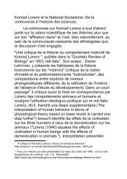
Paysages <strong>et</strong> <strong>communautés</strong> : <strong>Analyses</strong> <strong>multivariées</strong> <strong>des</strong> données spatialisées<br />
Analyse Canonique <strong>des</strong> Correspondances (CCA)<br />
Analyse de Redondance (RDA)<br />
Y<br />
X Y’<br />
Régression multiple<br />
Y’ = f (Y,X)<br />
Analyse 1<br />
Analyse 2<br />
Inertie <strong>des</strong> données<br />
biologiques seules (Y)<br />
Rapport <strong>des</strong> deux valeurs = inertie expliquée<br />
(Schéma simplifié)<br />
Inertie <strong>des</strong> données<br />
biologiques estimées<br />
(Y’) à partir de X<br />
(environnement)<br />
© 2007 Y.Del<strong>et</strong>tre & A. But<strong>et</strong>
<strong>Populations</strong> <strong>et</strong> <strong>communautés</strong> : <strong>Analyses</strong> <strong>multivariées</strong> de données spatialisées<br />
Average number of<br />
individuals<br />
14.00<br />
12.00<br />
10.00<br />
8.00<br />
6.00<br />
4.00<br />
2.00<br />
Eff<strong>et</strong> « qualité <strong>des</strong> haies » sur l’abondance<br />
<strong>des</strong> adultes de Diptères Chironomidae<br />
Sites A + B +C<br />
y = -2.7751Ln(x) + 16.511<br />
R 2 = 0.693<br />
0.00<br />
0 100 200 300 400 500 600<br />
Distance to the nearest brook<br />
0 225 675 m
<strong>Populations</strong> <strong>et</strong> <strong>communautés</strong> : <strong>Analyses</strong> <strong>multivariées</strong> de données spatialisées<br />
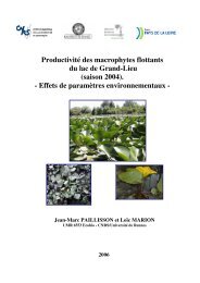
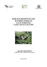
Eff<strong>et</strong> « qualité <strong>des</strong> haies » sur l’abondance<br />
<strong>des</strong> adultes de Diptères Chironomidae<br />
Descripteurs <strong>des</strong> haies AFC +<br />
Classification<br />
hiérarchique 6 types de haies<br />
T1 à T6<br />
1- largeur de la canopée<br />
2- perméabilité<br />
3- couvert arbustif<br />
4- couvert arborescent<br />
5- couvert herbacé<br />
6- largeur bande inculte<br />
7- largeur talus + fossé<br />
Average number of individuals<br />
per trap<br />
7.00<br />
6.00<br />
5.00<br />
4.00<br />
3.00<br />
2.00<br />
1.00<br />
0.00<br />
R 2 = 0.6605<br />
T5<br />
T2<br />
T3 T4<br />
0.00 0.50 1.00 1.50 2.00 2.50<br />
Average number of species per trap<br />
T6<br />
T1
<strong>Populations</strong> <strong>et</strong> <strong>communautés</strong> : <strong>Analyses</strong> <strong>multivariées</strong> de données spatialisées<br />
Eff<strong>et</strong> « qualité <strong>des</strong> haies » sur l’abondance<br />
<strong>des</strong> adultes de Diptères Chironomidae<br />
Nombre<br />
d’espèces <strong>et</strong><br />
nombre<br />
d’individus<br />
par piège dans<br />
chaque haie<br />
Descripteurs<br />
<strong>des</strong> haies<br />
CCA<br />
Variance extraite = 30.4% (1)<br />
Test de Monte Carlo : F-ratio<br />
- sur λ1 : 37.14, P < 0.01<br />
- overall : 5.31, P < 0.01<br />
Correlation – ratio :<br />
Largeur canopée : 0.426<br />
Largeur bande inculte : 0.341<br />
Couvert herbacé : 0.222<br />
Couvert arborescent : 0.221<br />
(1) Une fois l’eff<strong>et</strong> distance déduit (11.8%)
<strong>Populations</strong> <strong>et</strong> <strong>communautés</strong> : <strong>Analyses</strong> <strong>multivariées</strong> de données spatialisées<br />
Combinaison <strong>des</strong> variables environnementales <strong>et</strong> spatiales<br />
Community<br />
composition<br />
data table Y<br />
Environmental data<br />
matrix X<br />
= [a] [b] [c]<br />
[d] = Residuals<br />
Spatial data<br />
matrix W<br />
D’après Legendre, P. (décembre 2004, Rennes)
<strong>Populations</strong> <strong>et</strong> <strong>communautés</strong> : <strong>Analyses</strong> <strong>multivariées</strong> de données spatialisées<br />
Combinaison <strong>des</strong> variables environnementales <strong>et</strong> spatiales<br />
[d]= Residuals<br />
Response<br />
variable Explanatory table Explanatory table<br />
y<br />
a + b b+c<br />
X<br />
Environmental<br />
variables<br />
W<br />
Spatial<br />
base functions<br />
Environment X Spatial W<br />
[a] [b] [c]<br />
Décomposition<br />
de la variance<br />
par régressions<br />
partielles
<strong>Populations</strong> <strong>et</strong> <strong>communautés</strong> : <strong>Analyses</strong> <strong>multivariées</strong> de données spatialisées<br />
Combinaison <strong>des</strong> variables environnementales <strong>et</strong> spatiales<br />
Décomposition de la variance par régressions partielles<br />
Partial canonical analysis (CCA or RDA)<br />
• Spatial data = coordonnées Y <strong>et</strong> Y <strong>des</strong> échantillons<br />
• Calcul d’un polynome (souvent 3 e ordre)<br />
Z=b 1 x+b 2 y+b 3 x 2 +b 4 xy+b 5 y 2 +b 6 x 3 +b 7 x 2 y+b 8 xy 2 +b 9 y 3<br />
• Sélection pas-à-pas <strong>des</strong> termes du polynôme pour expliquer Y
<strong>Populations</strong> <strong>et</strong> <strong>communautés</strong> : <strong>Analyses</strong> <strong>multivariées</strong> de données spatialisées<br />
Combinaison <strong>des</strong> variables environnementales <strong>et</strong> spatiales<br />
Décomposition de la variance par régressions partielles<br />
Partial canonical analysis (CCA or RDA)<br />
Environmental data<br />
matrix X<br />
[a] [b] [c]<br />
Spatial data<br />
matrix<br />
W<br />
[d]= Residuals<br />
• On obtient (a) <strong>et</strong> (c) que l’on teste par permutations<br />
• La fraction (b), obtenue par différence, ne peut être testée<br />
• La fraction (d), non expliquée peut être quantifiée<br />
• On corrige les R² pour les biais.<br />
Note : ne jamais extrapoler au-delà <strong>des</strong> limites spatiales de l’étude !
<strong>Populations</strong> <strong>et</strong> <strong>communautés</strong> : <strong>Analyses</strong> <strong>multivariées</strong> de données spatialisées<br />
Combinaison <strong>des</strong> variables environnementales <strong>et</strong> spatiales<br />
Etude <strong>des</strong> <strong>communautés</strong> de poissons <strong>des</strong> coraux<br />
Mer <strong>des</strong> Caraïbes<br />
Bouchon-Navaro, Y., C. Bouchon, M. Louis & P. Legendre. 2004. Biogeographic patterns of<br />
coastal fish assemblages in the West Indies. Journal of Experimental Marine Biology and<br />
Ecology.
<strong>Populations</strong> <strong>et</strong> <strong>communautés</strong> : <strong>Analyses</strong> <strong>multivariées</strong> de données spatialisées<br />
Combinaison <strong>des</strong> variables environnementales <strong>et</strong> spatiales<br />
Etude <strong>des</strong> <strong>communautés</strong> de poissons <strong>des</strong> coraux<br />
Mer <strong>des</strong> Caraïbes<br />
Data: Fish community composition observed along underwater<br />
transects off 7 islands of the Caribbean arch.<br />
Sampling <strong>des</strong>ign: 248 underwater transects surveyed by a diver<br />
(visual census of 231 species).<br />
Questions<br />
• Is there a significant spatial pattern of community variation among<br />
the islands?<br />
• Is that pattern explained (in part) by environmental variables?<br />
Note: underwater visual censuses have high sampling variance.
<strong>Populations</strong> <strong>et</strong> <strong>communautés</strong> : <strong>Analyses</strong> <strong>multivariées</strong> de données spatialisées<br />
Combinaison <strong>des</strong> variables environnementales <strong>et</strong> spatiales<br />
Etude <strong>des</strong> <strong>communautés</strong> de poissons <strong>des</strong> coraux<br />
Mer <strong>des</strong> Caraïbes<br />
Variation in<br />
fish presence-absence<br />
=<br />
Habitat<br />
classes<br />
= 15.2%<br />
10.8%<br />
Residuals = 77.6%<br />
2.1%<br />
1.7%<br />
1.1%<br />
Depth = 3.9%<br />
Geographic gradients<br />
(Caribbean arch and<br />
latitude) = 8.4%<br />
5.9%<br />
0.6%<br />
0.1%
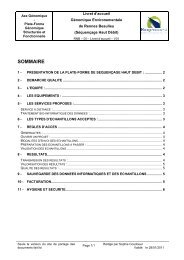
Paysage <strong>et</strong> <strong>communautés</strong> : <strong>Analyses</strong> <strong>multivariées</strong> de données spatialisées<br />
Dunes de Camargue<br />
• Dunes vastes <strong>et</strong> souvent très hautes, peu végétalisées<br />
• Bordées de sansouires, pas d’urbanisation adjacente<br />
• Très faible piétinement<br />
• Bien préservées de l’anthropisation<br />
© Comor, V., 2005<br />
Dune de Beauduc B
Paysage <strong>et</strong> <strong>communautés</strong> : <strong>Analyses</strong> <strong>multivariées</strong> de données spatialisées<br />
Dunes restaurées du Var<br />
• Dunes à ganivelles plus ou moins végétalisées <strong>et</strong> peu élevées<br />
• Très p<strong>et</strong>ites à assez longues<br />
• Forte urbanisation environnante<br />
© Comor, V., 2005<br />
Dune de l’Almanarre
Paysage <strong>et</strong> <strong>communautés</strong> : <strong>Analyses</strong> <strong>multivariées</strong> de données spatialisées<br />
Dunes dégradées du Var<br />
• Dunes sans ganivelles peu végétalisées <strong>et</strong> très planes<br />
• Peu étendues<br />
• Forte urbanisation environnante (constructions <strong>et</strong> milieux rudéraux)<br />
© Comor, V., 2005<br />
Dune de Cogolin
Caractérisation <strong>des</strong> sites<br />
Prise en compte de trois ensembles de facteurs à différentes échelles<br />
MORPHOLOGIE de la dune<br />
(échelle locale)<br />
PAYSAGE entourant la dune<br />
(échelle du paysage)<br />
• hauteur de la dune<br />
•arbres<br />
• largeur<br />
• bambous<br />
• longueur de la plage<br />
• couvert herbacé<br />
• taille du patch<br />
• halophiles<br />
• recouvrement végétal<br />
• eau<br />
•préservation<br />
•sable<br />
• matière organique<br />
• route/parking<br />
• granulométrie<br />
PERTURBATIONS<br />
• urbanisation<br />
• fréquentation de la plage<br />
• piétinement de la dune<br />
• ramassage <strong>des</strong> laisses de mer<br />
• ganivelles<br />
© Comor, V., 2005
Paysages <strong>et</strong> <strong>communautés</strong> : <strong>Analyses</strong> <strong>multivariées</strong> <strong>des</strong> données spatialisées<br />
Exemple de sortie<br />
graphique Analyse de<br />
Redondance (RDA)<br />
Sites (cercles, noms en gras)<br />
Espèces (triangles, noms en italiques)<br />
Variables explicatives (vecteurs)<br />
-0.6 0.8<br />
Herbe<br />
Urba<br />
Route/park<br />
Arbres<br />
Otior_ju<br />
Aleoch_2<br />
Trachy_a<br />
HYER-P HYER-P<br />
MOUL<br />
HYER-S<br />
Philop_p Philop_p<br />
Phaler_b Phaler_b<br />
PAMP-N<br />
Aleoch_1 Aleoch_1<br />
CABAS<br />
Stenos_i Stenos_i<br />
Anthicus<br />
Catom_co<br />
Cardio_a<br />
Tenter_m<br />
Xenon_tr<br />
BEAU-A<br />
Psamm_po<br />
Pimel_bi<br />
Psamm_ba<br />
Patch<br />
Ammob_ru<br />
Bledi_un<br />
Hdune<br />
© 2007 V. Comor & Y. Del<strong>et</strong>tre, Biodiversity & Conservation, in press<br />
-0.4 1.0<br />
© 2007 Y.Del<strong>et</strong>tre & A. But<strong>et</strong><br />
ALMA<br />
COGOL<br />
Xanthol<br />
Pleur_ca<br />
Thytt_se<br />
Chae_tib<br />
PAMP-S<br />
BRIAN<br />
PIEM<br />
© 2006 V. Comor<br />
VILLEP<br />
Tachyp_c<br />
Melig<strong>et</strong>h<br />
Harpal<br />
GRAC<br />
BEAU-B BEAU-B<br />
Psyll_ma<br />
Halam_pe<br />
Crytoph<br />
Phaler_p
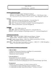
Paysages <strong>et</strong> <strong>communautés</strong> : <strong>Analyses</strong> <strong>multivariées</strong> <strong>des</strong> données spatialisées<br />
Partition de variance sur les abondances d’espèces sabulicoles<br />
Structure <strong>des</strong> <strong>communautés</strong> de coléoptères semble régie par la<br />
morphologie dunaire (échelle locale)<br />
Facteurs très tr s locaux qui interagissent avec <strong>des</strong> espèces esp ces très tr s spécialis sp cialisées es<br />
© Comor, V., 2005<br />
Variance totale expliquée = 75.61%<br />
RDA<br />
Morpho<br />
50.90% **<br />
0.05%<br />
0.19%<br />
1.71% 11.4% 4.18%<br />
Perturb Paysage<br />
7.18%<br />
Résidus = 24.39%
Résultats : Relations avec les facteurs environnementaux<br />
Partition de variance sur les abondances d’espèces généralistes<br />
Variance totale expliquée = 64.31%<br />
RDA<br />
Morpho<br />
1.39%<br />
6.01%<br />
9.96%<br />
17.47% 1.04% 23.87% **<br />
Perturb Paysage<br />
4.55%<br />
Résidus = 35.69%<br />
Influence prépondérante du paysage environnant <strong>et</strong> impact plus important<br />
<strong>des</strong> perturbations sur les allochtones malgré le faible nombre d’individus<br />
• Perte <strong>des</strong> caractéristiques propres de la dune<br />
• Homogénéisation avec le paysage environnant<br />
Installation<br />
d’espèces<br />
allochtones<br />
20
<strong>Populations</strong> <strong>et</strong> <strong>communautés</strong> : <strong>Analyses</strong> <strong>multivariées</strong> de données spatialisées<br />
Relations espèces – environnement<br />
1. Utilisation de la régression multiple (CCA, RDA)<br />
• CCA <strong>et</strong> RDA : méthode d’AFC / ACP<br />
• Partial Canonical Analysis Variance partitionning<br />
2. Utilisation de la co-variance (méthode de Co-Inertie)
<strong>Populations</strong> <strong>et</strong> <strong>communautés</strong> : <strong>Analyses</strong> <strong>multivariées</strong> de données spatialisées<br />
Variables à<br />
expliquer<br />
(espèces)<br />
ACP, AFC ou ACM<br />
Espace factoriel<br />
<strong>des</strong> espèces<br />
Co-Inertie – Etape 1<br />
Variables<br />
explicatives<br />
(environnement)<br />
ACP, AFC ou ACM<br />
Espace factoriel<br />
environnement
<strong>Populations</strong> <strong>et</strong> <strong>communautés</strong> : <strong>Analyses</strong> <strong>multivariées</strong> de données spatialisées<br />
Espace factoriel<br />
<strong>des</strong> espèces<br />
Co-Inertie – Etape 2<br />
Espace factoriel de<br />
co-inertie<br />
espace commun<br />
aux 2 analyses<br />
Espace factoriel<br />
environnement
<strong>Populations</strong> <strong>et</strong> <strong>communautés</strong> : <strong>Analyses</strong> <strong>multivariées</strong> de données spatialisées<br />
Co-Inertie – Etape 2<br />
La co-inertie recherche une représentation <strong>des</strong> deux<br />
ensembles de données dans un espace commun (1)<br />
Principe : Maximise les corrélations entre les<br />
coordonnées <strong>des</strong> sites issus <strong>des</strong> deux analyses<br />
précédentes (maximisation de la covariance).<br />
Mode opératoire : En maintenant fixe l’espace <strong>des</strong><br />
espèces (Y), elle recherche de nouveau axes dans<br />
l’espace <strong>des</strong> facteurs (X) remplissant ces conditions.<br />
(1) représentation de la co-structure
<strong>Populations</strong> <strong>et</strong> <strong>communautés</strong> : <strong>Analyses</strong> <strong>multivariées</strong> de données spatialisées<br />
Situation de départ<br />
HB<br />
CHP<br />
CHB<br />
HP F2<br />
5<br />
BP<br />
CP<br />
CB<br />
5<br />
F1<br />
BB<br />
Faune<br />
ACP faune de la végétation<br />
HB<br />
HP<br />
BB<br />
Milie<br />
u<br />
Co-Inertie – approche simplifiée<br />
F2<br />
CHB<br />
BP<br />
CB<br />
CP<br />
CHP<br />
F1<br />
ACM facteurs environnement<br />
inchangé<br />
rotation<br />
inversion<br />
HB<br />
CHP<br />
CHB<br />
CP CB<br />
BP<br />
CHB<br />
F1<br />
CHP<br />
HP F2<br />
HP<br />
5<br />
BP<br />
CP<br />
CB<br />
HB<br />
5<br />
Milieu<br />
F2<br />
BB<br />
F1<br />
BB<br />
Faune<br />
Situation<br />
d'arrivée<br />
HB<br />
CPCB<br />
BP<br />
CHB<br />
F1<br />
CHP CHP<br />
CHB<br />
HP<br />
5<br />
F2<br />
HB<br />
HP<br />
BP<br />
CP<br />
Milie 5<br />
CB<br />
u<br />
BB<br />
BB<br />
Faune<br />
F2<br />
superposition
<strong>Populations</strong> <strong>et</strong> <strong>communautés</strong> : <strong>Analyses</strong> <strong>multivariées</strong> de données spatialisées<br />
Co-Inertie – approche simplifiée<br />
Double représentation "approchée"<br />
BB<br />
F2<br />
Faune<br />
5<br />
Milieu<br />
BP<br />
CB<br />
CP<br />
5<br />
HB F2 HP<br />
HP<br />
CHB<br />
CHP CHP<br />
F1<br />
CHB<br />
BP<br />
CB CP<br />
HB<br />
Double représentation ADE-4<br />
BB<br />
BP<br />
CB<br />
CHB CHP<br />
HB<br />
CP<br />
HP
<strong>Populations</strong> <strong>et</strong> <strong>communautés</strong> : <strong>Analyses</strong> <strong>multivariées</strong> de données spatialisées<br />
Photo-interprétation<br />
imagerie satellitaire<br />
Co-Inertie – Exemple 1<br />
Composition du paysage<br />
1 – Longueur <strong>des</strong> haies (m/ha)<br />
2 – Surface <strong>des</strong> boisements (%)<br />
3 – Prairies permanentes (%)<br />
4 – Maïs (%)<br />
5 – Autres cultures (%)<br />
ACP<br />
10 unités paysagères<br />
Photo aérienne IGN Structure bocagère Occupation du sol<br />
Abondance <strong>des</strong> Carabidae<br />
– 110 haies, 330 pièges<br />
– de mai à juill<strong>et</strong> 1988<br />
– 73 espèces, # 5000 individus<br />
AFC
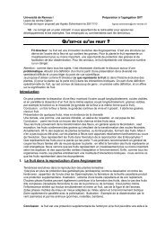
<strong>Populations</strong> <strong>et</strong> <strong>communautés</strong> : <strong>Analyses</strong> <strong>multivariées</strong> de données spatialisées<br />
Analyse de co-inertie<br />
Isolement <strong>des</strong> sites<br />
« intensifiés » (2,4,6,10).<br />
Sites riches en bois ou haies<br />
forment un groupe distinct<br />
(1,3,5,8,9,11).<br />
Le site 7 est totalement isolé<br />
<strong>des</strong> autres (bocage ancien<br />
non remanié).<br />
Les sites s’organisent suivant<br />
le double gradient <strong>des</strong><br />
facteurs environnementaux :<br />
intensification (A) <strong>et</strong><br />
homogénéisation(B).<br />
Cohérence / différentiation<br />
<strong>des</strong> sites selon la double<br />
représentation<br />
(facteurs/espèces).<br />
Co-Inertie – Exemple 1<br />
Decreasing total abundance<br />
3.1<br />
-2.3 2<br />
-1.6<br />
7<br />
8<br />
1<br />
11<br />
9<br />
F2<br />
5<br />
3<br />
10<br />
A<br />
B<br />
Increasing number of small species<br />
4<br />
6<br />
2<br />
F1
<strong>Populations</strong> <strong>et</strong> <strong>communautés</strong> : <strong>Analyses</strong> <strong>multivariées</strong> de données spatialisées<br />
Co-Inertie – Exemple 2
<strong>Populations</strong> <strong>et</strong> <strong>communautés</strong> : <strong>Analyses</strong> <strong>multivariées</strong> de données spatialisées<br />
Co-Inertie – Exemple 2<br />
Micro-mammifères (ACP)<br />
• Abondance <strong>des</strong> espèces de rongeurs <strong>et</strong><br />
musaraignessur trois types de digues<br />
Environnement (ACP)<br />
• Physionomie <strong>des</strong> digues<br />
• Composition de la mosaïque agricole<br />
dans un rayon de 500m autour <strong>des</strong><br />
digues<br />
Co-inertie
<strong>Populations</strong> <strong>et</strong> <strong>communautés</strong> : <strong>Analyses</strong> <strong>multivariées</strong> de données spatialisées<br />
6,3 % of co-inertia<br />
F1<br />
2<br />
1<br />
7<br />
1<br />
2<br />
2<br />
6<br />
6<br />
1<br />
3<br />
2<br />
1<br />
Co-Inertie – Exemple 2<br />
2<br />
5<br />
14<br />
1<br />
6<br />
15<br />
18<br />
17<br />
F2<br />
10<br />
90,3 % of co-inertia<br />
3.<br />
-<br />
-<br />
2<br />
1.<br />
3 2<br />
3.2<br />
2<br />
3 0<br />
9<br />
2<br />
5<br />
2<br />
1<br />
7<br />
4 2<br />
1<br />
2<br />
8<br />
1 4<br />
9<br />
23<br />
1<br />
-4 4<br />
-1.5<br />
Grass<br />
M<br />
g<br />
Pea<br />
Cereal<br />
Meadow<br />
Ms<br />
F2<br />
Veg<strong>et</strong><br />
Bramble<br />
Ivy<br />
Litter<br />
Connect Shrub<br />
Bare G. Tree<br />
Ploughed<br />
Maize<br />
Sc<br />
S<br />
Crm<br />
F1<br />
A<br />
As<br />
Cg
<strong>Populations</strong> <strong>et</strong> <strong>communautés</strong> : <strong>Analyses</strong> <strong>multivariées</strong> <strong>des</strong> données spatialisées<br />
© 2005-2007, Y.R. Del<strong>et</strong>tre, UMR 6553 ECOBIO, Rennes