Contribution à la conception optimale en terme de linéarité et ...
Contribution à la conception optimale en terme de linéarité et ...
Contribution à la conception optimale en terme de linéarité et ...

Create successful ePaper yourself
Turn your PDF publications into a flip-book with our unique Google optimized e-Paper software.
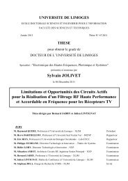
C/(N+I) (dB)<br />
CHAPITRE III - METHODOLOGIE DE CONCEPTION OPTMALE EN TERME DE LINEARITE ET DE CONSOMMATION<br />
Nous avons suivi <strong>la</strong> même procédure <strong>à</strong> l’harmonique 2 mais <strong>en</strong> fixant l’impédance <strong>de</strong><br />
charge au fondam<strong>en</strong>tale sur l’impédance <strong>optimale</strong> <strong>de</strong> r<strong>en</strong><strong>de</strong>m<strong>en</strong>t. Nous pouvons voir que l<strong>à</strong><br />
<strong>en</strong>core que <strong>la</strong> courbe <strong>optimale</strong> <strong>et</strong> celle obt<strong>en</strong>ue avec l’impédance <strong>optimale</strong> <strong>de</strong> r<strong>en</strong><strong>de</strong>m<strong>en</strong>t <strong>à</strong> 2f0<br />
sont proches l’une <strong>de</strong> l’autre. Elles sont tracées <strong>en</strong> bleu (Figure III.27). Nous pouvons <strong>en</strong><br />
déduire que les conditions <strong>de</strong> charge <strong>optimale</strong> selon ce critère <strong>et</strong> pour c<strong>et</strong>te technologie<br />
correspond<strong>en</strong>t aux conditions <strong>optimale</strong>s <strong>de</strong> r<strong>en</strong><strong>de</strong>m<strong>en</strong>t.<br />
Afin d’évaluer quantitativem<strong>en</strong>t l’influ<strong>en</strong>ce <strong>de</strong> l’impédance <strong>de</strong> charge <strong>à</strong> l’harmonique<br />
2, nous avons égalem<strong>en</strong>t tracé une courbe <strong>en</strong> le court-circuitant <strong>en</strong> sortie du transistor (Figure<br />
III.27). Le rapport / N a été augm<strong>en</strong>té <strong>de</strong> près <strong>de</strong> 1 dB. Ceci correspond <strong>à</strong> une<br />
P dc<br />
dégradation <strong>de</strong> près <strong>de</strong> 25% sur <strong>la</strong> consommation <strong>de</strong> l’amplificateur.<br />
24<br />
22<br />
20<br />
18<br />
16<br />
14<br />
12<br />
10<br />
Enveloppe <strong>optimale</strong> <strong>à</strong> 2f0 Enveloppe pour impédance <strong>optimale</strong> <strong>de</strong> r<strong>en</strong><strong>de</strong>m<strong>en</strong>t <strong>à</strong> 2f0<br />
Enveloppe pour un court circuit <strong>à</strong> 2f0<br />
15 18 21 24 27 30<br />
Pdc/N (dB)<br />
Figure III.27 - Influ<strong>en</strong>ce <strong>de</strong>s impédances <strong>de</strong> charge <strong>à</strong> 2f0<br />
III.4.3.1.2. - Impédances <strong>de</strong> source<br />
Nous avons cherché <strong>à</strong> optimiser l’impédance <strong>de</strong> source <strong>à</strong> 2f0. Les impédances <strong>de</strong><br />
charge au fondam<strong>en</strong>tale <strong>et</strong> <strong>à</strong> l’harmonique 2 ont été fixées sur les impédances <strong>optimale</strong>s <strong>de</strong><br />
r<strong>en</strong><strong>de</strong>m<strong>en</strong>t.<br />
117