FONCTION LOGARITHME NEPERIEN - maths et tiques
FONCTION LOGARITHME NEPERIEN - maths et tiques
FONCTION LOGARITHME NEPERIEN - maths et tiques

You also want an ePaper? Increase the reach of your titles
YUMPU automatically turns print PDFs into web optimized ePapers that Google loves.
<strong>FONCTION</strong> <strong>LOGARITHME</strong><br />
<strong>NEPERIEN</strong><br />
En 1614, un mathématicien écossais, John Napier (1550 ; 1617) cicontre,<br />
plus connu sous le nom francisé de Neper publie « Mirifici<br />
logarithmorum canonis descriptio ».<br />
Dans c<strong>et</strong> ouvrage, qui est la finalité d’un travail de 20 ans,<br />
Neper présente un outil perm<strong>et</strong>tant de simplifier les calculs<br />
opératoires : le logarithme.<br />
Toutefois c<strong>et</strong> outil ne trouvera son essor qu’après la mort de Neper.<br />
Les mathématiciens anglais Henri Briggs (1561 ; 1630) <strong>et</strong> William<br />
Oughtred (1574 ; 1660) reprennent <strong>et</strong> prolongent les travaux<br />
de Neper.<br />
Les mathématiciens de l’époque établissent alors des tables de logarithmes de plus en plus<br />
précises.<br />
L’intérêt d’établir ces tables logarithmiques est de perm<strong>et</strong>tre de substituer une multiplication<br />
par une addition (paragraphe II). Ceci peut paraître dérisoire aujourd’hui, mais il faut<br />
comprendre qu’à c<strong>et</strong>te époque, les calculatrices n’existent évidemment pas, les nombres<br />
décimaux ne sont pas d’usage courant <strong>et</strong> les opérations posées telles que nous les utilisons ne<br />
sont pas encore connues. Et pourtant l'astronomie, la navigation ou le commerce demandent<br />
d’effectuer des opérations de plus en plus complexes.<br />
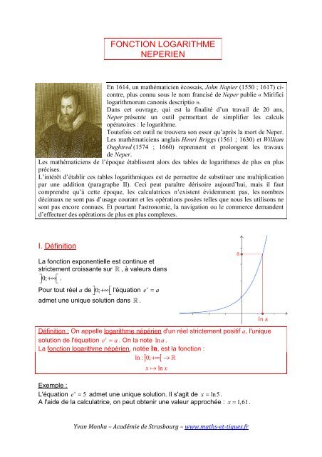
I. Définition<br />
La fonction exponentielle est continue <strong>et</strong><br />
strictement croissante sur ℝ , à valeurs dans<br />
0;+∞ ⎤⎦ ⎡⎣ .<br />
Pour tout réel a de ⎤⎦ 0;+∞ ⎡⎣ l'équation e x = a<br />
adm<strong>et</strong> une unique solution dans ℝ .<br />
Définition : On appelle logarithme népérien d'un réel strictement positif a, l'unique<br />
solution de l'équation e x = a . On la note ln a .<br />
La fonction logarithme népérien, notée ln, est la fonction :<br />
ln : 0; +∞ → ℝ<br />
] [<br />
x ֏ ln x<br />
Exemple :<br />
L'équation e x = 5 adm<strong>et</strong> une unique solution. Il s'agit de x = ln5.<br />
A l'aide de la calculatrice, on peut obtenir une valeur approchée :<br />
x ≈ 1,61.<br />
Yvan Monka – Académie de Strasbourg – www.<strong>maths</strong>-<strong>et</strong>-<strong>tiques</strong>.fr
Remarque :<br />
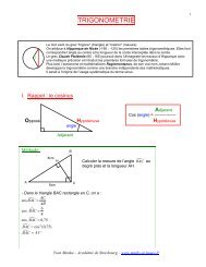
Les courbes représentatives des fonctions exponentielle <strong>et</strong> logarithme népérien sont<br />
symétriques par rapport à la droite d'équation y = x .<br />
Conséquences :<br />
y<br />
a) y = ln x avec x > 0 ⇔ x = e<br />
1<br />
b) ln1 = 0 ; lne = 1 ; ln = −1<br />
e<br />
c) Pour tout x, lne x = x<br />
d) Pour tout x positif, e ln x = x<br />
Démonstrations :<br />
a) Par définition<br />
b) - Car e 0 = 1<br />
- Car e 1 = e<br />
- Car e −1 = 1<br />
e<br />
c) Si on pose y = e x , alors<br />
x = ln y = lnex<br />
d) Si on pose y = ln x , alors x = e y ln x<br />
= e<br />
Exemples : e ln 2 = 2 <strong>et</strong> lne 4 = 4<br />
Propriété : Pour tous réels x <strong>et</strong> y strictement positifs, on a :<br />
a) ln x = ln y ⇔ x = y<br />
b) ln x < ln y ⇔ x < y<br />
Démonstration :<br />
a) x = y ⇔ eln x = e ln y ⇔ ln x = ln y<br />
b) x < y ⇔ eln x < e ln y ⇔ ln x < ln y<br />
Yvan Monka – Académie de Strasbourg – www.<strong>maths</strong>-<strong>et</strong>-<strong>tiques</strong>.fr
Méthode : Résoudre une équation ou une inéquation<br />
Résoudre dans ℝ les équations <strong>et</strong> inéquations suivantes :<br />
a) ln x = 2 b) e x +1 = 5 c) 3ln x − 4 = 8<br />
ln 6x −1 ≥ 2<br />
e) e x + 5 > 4e x<br />
d) ( )<br />
a) ln x = 2<br />
⇔ ln x = lne 2<br />
⇔ x = e 2<br />
b) e x +1 = 5<br />
⇔ e x +1 = e ln5<br />
⇔ x + 1 = ln5<br />
⇔ x = ln5 − 1<br />
c) 3ln x − 4 = 8<br />
⇔ 3ln x = 12<br />
⇔ ln x = 4<br />
⇔ ln x = ln e 4<br />
⇔ x = e 4<br />
d) ln ( 6x −1) ≥ 2<br />
2<br />
⇔ ln ( 6x −1) ≥ ln e<br />
⇔ 6x −1 ≥ e<br />
2<br />
e + 1<br />
⇔ x ≥<br />
6<br />
e) e x + 5 > 4e x<br />
x x<br />
⇔ e − 4e > −5<br />
x<br />
⇔ − 3e > −5<br />
x<br />
⇔ e <<br />
5<br />
3<br />
⎛ 5 ⎞<br />
ln<br />
x<br />
⎜ ⎟<br />
⎝ 3 ⎠ e e<br />
⇔ <<br />
2<br />
La solution est e 2 .<br />
La solution est ln5 − 1.<br />
La solution est e 4 .<br />
L'ensemble solution est donc<br />
⎛ 5 ⎞<br />
⇔ x < ln ⎜ ⎟<br />
⎝ 3 ⎠<br />
⎤ ⎛ 5 ⎞⎡<br />
L'ensemble solution est donc ⎥−∞;ln ⎜ ⎟<br />
3<br />
⎢<br />
⎦ ⎝ ⎠⎣<br />
.<br />
e 2 + 1<br />
6 ;+∞<br />
⎡ ⎡<br />
⎢ ⎢ .<br />
⎣ ⎣<br />
Yvan Monka – Académie de Strasbourg – www.<strong>maths</strong>-<strong>et</strong>-<strong>tiques</strong>.fr
II. Propriété de la fonction logarithme népérien<br />
1) Relation fonctionnelle<br />
Théorème : Pour réel x <strong>et</strong> y strictement positif, on a : ( )<br />
ln x× y = ln x + ln y<br />
Remarque : C<strong>et</strong>te formule perm<strong>et</strong> de transformer un produit en somme.<br />
Démonstration :<br />
eln( x × y) = x × y = e ln x × e ln y ln x + ln y<br />
= e<br />
ln x× y = ln x + ln y<br />
Donc ( )<br />
Corollaires : Pour tous réels x <strong>et</strong> y strictement positifs, on a :<br />
a) ln 1<br />
= − ln x<br />
x<br />
b) ln x<br />
= ln x − ln y<br />
y<br />
c)<br />
ln x = 1<br />
ln x<br />
2<br />
ln<br />
n<br />
x = n ln x avec n entier relatif<br />
d) ( )<br />
Démonstrations :<br />
1 ⎛ 1 ⎞<br />
a) ln + ln x = ln ⎜ × x ⎟ = ln1 = 0<br />
x ⎝ x ⎠<br />
x ⎛ 1 ⎞ 1<br />
b) ln = ln ⎜ x× ⎟ = ln x + ln = ln x − ln y<br />
y ⎝ y ⎠ y<br />
c) ( )<br />
2ln x = ln x + ln x = ln x × x = ln x<br />
n n<br />
ln(<br />
x )<br />
e = e = x = e<br />
d)<br />
nln x ( ln x ) n<br />
n<br />
Donc n ln x = ln ( x )<br />
Exemples :<br />
⎛ 1 ⎞<br />
a) ln ⎜ ⎟ = −ln<br />
2<br />
⎝ 2 ⎠<br />
b)<br />
⎛ 3 ⎞<br />
ln ⎜ ⎟ = ln 3− ln 4<br />
⎝ 4 ⎠<br />
Méthode : Simplifier une expression<br />
Yvan Monka – Académie de Strasbourg – www.<strong>maths</strong>-<strong>et</strong>-<strong>tiques</strong>.fr<br />
c)<br />
ln 5 = 1<br />
A = ln ( 3 − 5) + ln ( 3+ 5)<br />
B = 3ln2 + ln5 − 2ln3<br />
ln 64 = ln 8 = 2ln8<br />
2 ln5 d) 2 ( )<br />
C = lne 2 − ln 2<br />
e
ln ( 3 5) ln ( 3 5)<br />
( )( )<br />
A = − + +<br />
= ln 3 − 5 3+ 5<br />
( )<br />
= ln 9 − 5<br />
= ln 4<br />
B = 3ln2 + ln5 − 2ln3<br />
= ln2 3 + ln5 − ln3 2<br />
= ln 23 × 5<br />
3 2<br />
= ln 40<br />
9<br />
Méthode : Résoudre une équation ou une inéquation<br />
1) Résoudre dans ℝ l’équation : 6 x = 2<br />
2) Résoudre dans ⎤⎦ 0;+∞ ⎡⎣ l'équation : x 5 = 3<br />
C = lne 2 − ln 2<br />
e<br />
= 2ln e − ln2 + ln e<br />
= 2 − ln2 + 1<br />
= 3− ln2<br />
3) 6 augmentations successives de t % correspondent à une augmentation globale<br />
de 30 %. Donner une valeur approchée de t.<br />
1) 6 x = 2<br />
x<br />
⇔ ln 6 = ln 2<br />
( )<br />
⇔ x ln 6 = ln 2<br />
⇔ x =<br />
ln 6<br />
ln 2<br />
2) Comme x > 0 , on a :<br />
x 5 = 3<br />
5 ( x )<br />
⇔ ln = ln 3<br />
⇔ 5ln x = ln 3<br />
1<br />
⇔ ln x = ln 3<br />
5<br />
1<br />
⎛ ⎞<br />
5<br />
⇔ ln x = ln ⎜3 ⎟<br />
⎝ ⎠<br />
1<br />
5<br />
⇔ x = 3<br />
5 La solution est 3 .<br />
1<br />
La solution est<br />
ln6<br />
ln 2 .<br />
1<br />
5 5<br />
Remarque : 3 se lit "racine cinquième de 3" <strong>et</strong> peut se noter 3<br />
3) Le problème revient à résoudre dans ⎤⎦ 0;+∞ ⎡⎣ l'équation :<br />
Yvan Monka – Académie de Strasbourg – www.<strong>maths</strong>-<strong>et</strong>-<strong>tiques</strong>.fr<br />
.<br />
⎛ t ⎞<br />
⎜1+ ⎟ = 1,3<br />
⎝ 100 ⎠<br />
6
⎛ t ⎞<br />
⇔ ln ⎜1+ ⎟ = ln1,3<br />
⎝ 100 ⎠<br />
⎛ t ⎞<br />
⇔ 6ln ⎜1+ ⎟ = ln1,3<br />
⎝ 100 ⎠<br />
⎛ t ⎞ 1<br />
⇔ ln ⎜1+ ⎟ = ln1,3<br />
⎝ 100 ⎠ 6<br />
1<br />
⎛ t ⎞ ⎛ ⎞<br />
6<br />
⇔ ln ⎜1+ ⎟ = ln ⎜1,3 ⎟<br />
⎝ 100 ⎠ ⎝ ⎠<br />
6<br />
1<br />
t 6<br />
⇔ 1+ = 1,3<br />
100<br />
1<br />
⎛ ⎞ 6<br />
⇔ t = 100⎜1,3 −1⎟ ≈ 4,5<br />
⎝ ⎠<br />
Une augmentation globale de 30 % correspond à 6 augmentations successives<br />
d'environ 4,5 %.<br />
III. Etude de la fonction logarithme népérien<br />
1) Continuité <strong>et</strong> dérivabilité<br />
Propriété : La fonction logarithme népérien est continue sur ⎤⎦ 0;+∞ ⎡⎣ .<br />
- Admis -<br />
Propriété : La fonction logarithme népérien est dérivable sur ⎤⎦ 0;+∞ ⎡⎣ <strong>et</strong><br />
Yvan Monka – Académie de Strasbourg – www.<strong>maths</strong>-<strong>et</strong>-<strong>tiques</strong>.fr<br />
(ln x)' = 1<br />
x .<br />
Démonstration :<br />
Nous adm<strong>et</strong>tons que la fonction logarithme népérien est dérivable sur ⎤⎦ 0;+∞ ⎡⎣ .<br />
Posons f (x) = eln x .<br />
Alors f '(x) = (ln x)'eln x = x(ln x)'<br />
Comme f (x) = x , on a f '(x) = 1.<br />
Donc<br />
Exemple :<br />
x(ln x)' = 1 <strong>et</strong> donc<br />
(ln x)' = 1<br />
x .<br />
Dériver la fonction suivante sur l'intervalle ⎤⎦ 0;+∞ ⎡⎣ :<br />
f '(x) =<br />
1<br />
× x − ln x × 1<br />
x<br />
x 2 = 1− ln x<br />
x 2<br />
f (x) =<br />
ln x<br />
x
2) Variations<br />
Propriété : La fonction logarithme népérien est strictement croissante sur ⎤⎦ 0;+∞ ⎡⎣ .<br />
Démonstration :<br />
Pour tout réel x > 0,<br />
3) Convexité<br />
(ln x)' = 1<br />
> 0 .<br />
x<br />
Propriété : La fonction logarithme népérien est concave sur ⎤⎦ 0;+∞ ⎡⎣ .<br />
Démonstration :<br />
Pour tout réel x > 0,<br />
(ln x)' = 1<br />
x .<br />
1<br />
(ln x)'' = − < 0 donc la dérivée de la fonction ln est strictement décroissante sur<br />
2<br />
x 0;+∞ ⎤⎦ ⎡⎣ <strong>et</strong> donc la fonction logarithme népérien est concave sur c<strong>et</strong> intervalle.<br />
4) Limites aux bornes<br />
Propriété : lim ln x = +∞ <strong>et</strong><br />
x→+∞<br />
lim ln x = −∞<br />
x→0<br />
x>0<br />
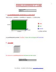
On peut justifier ces résultats par symétrie de la<br />
courbe représentative de la fonction exponentielle.<br />
5) Tangentes particulières<br />
Rappel : Une équation de la tangente à la courbe C f au point d'abscisse a est :<br />
( )<br />
y = f '( a) x − a + f ( a)<br />
.<br />
Dans le cas de la fonction logarithme népérien, l'équation est de la forme :<br />
1<br />
y = ( x − a) + ln a .<br />
a<br />
Yvan Monka – Académie de Strasbourg – www.<strong>maths</strong>-<strong>et</strong>-<strong>tiques</strong>.fr
- Au point d'abscisse 1, l'équation de la tangente est y ( x )<br />
- Au point d'abscisse e, l'équation de la tangente est ( )<br />
6) Courbe représentative<br />
1<br />
=<br />
1<br />
− 1 + ln1 soit : y = x − 1.<br />
1<br />
y =<br />
e<br />
x − e + ln e soit : y = 1<br />
x .<br />
e<br />
On dresse le tableau de variations de la fonction logarithme népérien :<br />
Valeurs particulières :<br />
x 0 +∞<br />
ln'(x) ⎪⎪ +<br />
+∞<br />
ln x<br />
−∞<br />
ln1 = 0<br />
lne = 1<br />
Méthode : Etudier les variations d'une fonction<br />
1) Déterminer les variations de la fonction f définie sur ⎤⎦ 0;+∞ ⎡⎣ par<br />
f (x) = 3 − x + 2ln x .<br />
2) Etudier la convexité de la fonction f.<br />
Yvan Monka – Académie de Strasbourg – www.<strong>maths</strong>-<strong>et</strong>-<strong>tiques</strong>.fr
1) Sur ⎤⎦ 0;+∞ ⎡⎣ , on a f '(x) = −1+ 2 2 − x<br />
= .<br />
x x<br />
Comme x > 0 , f '(x) est du signe de 2 − x .<br />
La fonction f est donc strictement croissante sur ⎤⎦ 0;2⎤⎦<br />
<strong>et</strong> strictement décroissante<br />
sur ⎡⎣ 2;+∞ ⎡⎣ .<br />
On dresse le tableau de variations :<br />
x 0 2 +∞<br />
f '(x) ⎪⎪ + 0 -<br />
f (x)<br />
f (2) = 3− 2 + 2ln 2 = 1+ 2ln 2<br />
1+ 2ln 2<br />
( )<br />
− 1× x − 2 − x × 1 −x − 2 + x 2<br />
2) Sur ⎤⎦ 0;+∞ ⎡⎣ , on a f ''( x)<br />
= = = − < 0.<br />
2 2 2<br />
x x x<br />
La fonction f ' est donc décroissante sur 0;+∞ ⎤⎦ ⎡⎣ . On en déduit que la fonction f est<br />
concave sur ⎤⎦ 0;+∞ ⎡⎣ .<br />
IV. Positions relatives<br />
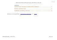
Propriété : La courbe représentative de la fonction exponentielle est au-dessus de la<br />
droite d'équation y = x .<br />
La droite d'équation y = x est au-dessus de la courbe représentative de la fonction<br />
logarithme népérien.<br />
Yvan Monka – Académie de Strasbourg – www.<strong>maths</strong>-<strong>et</strong>-<strong>tiques</strong>.fr
Démonstration :<br />
- On considère la fonction f définie sur ℝ par f (x) = ex − x .<br />
f '(x) = ex − 1.<br />
f '(x) = 0<br />
⇔ e x − 1 = 0<br />
⇔ e x = 1<br />
⇔ x = 0<br />
On a également f (0) = e0 − 0 = 1 > 0 .<br />
On dresse ainsi le tableau de variations :<br />
x −∞ 0 +∞<br />
f '(x) - 0 +<br />
f (x)<br />
On en déduit que pour tout x de ℝ , on a f (x) = ex − x > 0 soit e x > x<br />
- On considère la fonction g définie sur ⎤⎦ 0;+∞ ⎡⎣ par<br />
g '(x) = 1− 1 x − 1<br />
= .<br />
x x<br />
Comme x > 0 , f '(x) est du signe de x − 1.<br />
On a également g(1) = 1− ln1 = 1 > 0 .<br />
On dresse ainsi le tableau de variations :<br />
Yvan Monka – Académie de Strasbourg – www.<strong>maths</strong>-<strong>et</strong>-<strong>tiques</strong>.fr<br />
1<br />
g(x) = x − ln x .<br />
x 0 1 +∞<br />
g '(x) - 0 +<br />
g(x)<br />
On en déduit que pour tout x de ⎤⎦ 0;+∞ ⎡⎣ , on a g(x) = x − ln x > 0 soit x > ln x .<br />
1<br />
Hors du cadre de la classe, aucune reproduction, même partielle, autres que celles prévues à l'article L 122-5 du<br />
code de la propriété intellectuelle, ne peut être faite de ce site sans l'autorisation expresse de l'auteur.<br />
www.<strong>maths</strong>-<strong>et</strong>-<strong>tiques</strong>.fr/index.php/mentions-legales