Contributions à l'étude de la classification spectrale et applications

2.3.4 Classification via l’opérateur de la chaleur dans R p 49
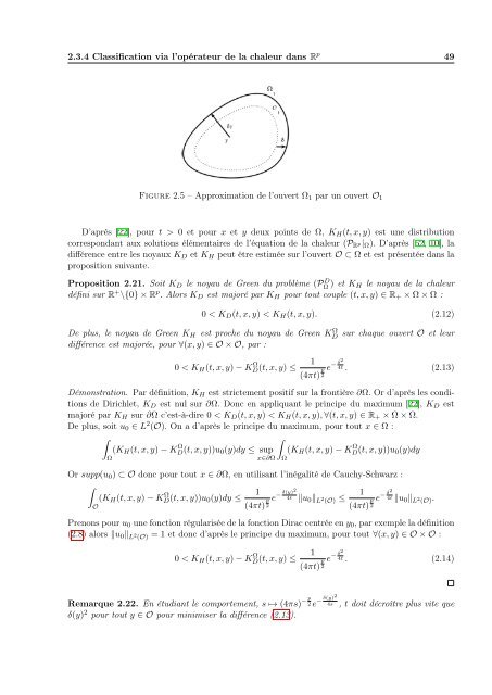
Figure 2.5 – Approximation de l’ouvert Ω1 par un ouvert O1
D’après [22], pour t > 0 et pour x et y deux points de Ω, KH(t, x, y) est une distribution
correspondant aux solutions élémentaires de l’équation de la chaleur (PR p|Ω). D’après [62, 10], la
différence entre les noyaux KD et KH peut être estimée sur l’ouvert O ⊂ Ω et est présentée dans la
proposition suivante.
Proposition 2.21. Soit KD le noyau de Green du problème (P D Ω ) et KH le noyau de la chaleur
défini sur R + \{0} × R p . Alors KD est majoré par KH pour tout couple (t, x, y) ∈ R+ × Ω × Ω :
0 < KD(t, x, y) < KH(t, x, y). (2.12)
De plus, le noyau de Green KH est proche du noyau de Green K Ω D
différence est majorée, pour ∀(x, y) ∈ O × O, par :
0 < KH(t, x, y) − K Ω D(t, x, y) ≤
sur chaque ouvert O et leur
1
(4πt) p
δ2
−
e 4t . (2.13)
2
Démonstration. Par définition, KH est strictement positif sur la frontière ∂Ω. Or d’après les conditions
de Dirichlet, KD est nul sur ∂Ω. Donc en appliquant le principe du maximum [22], KD est
majoré par KH sur ∂Ω c’est-à-dire 0 < KD(t, x, y) < KH(t, x, y), ∀(t, x, y) ∈ R+ × Ω × Ω.
De plus, soit u0 ∈ L2 (O). On a d’après le principe du maximum, pour tout x ∈ Ω :
(KH(t, x, y) − K Ω
D(t, x, y))u0(y)dy ≤ sup (KH(t, x, y) − K
x∈∂Ω
Ω D(t, x, y))u0(y)dy
Ω
Or supp(u0) ⊂ O donc pour tout x ∈ ∂Ω, en utilisant l’inégalité de Cauchy-Schwarz :
(KH(t, x, y) − K Ω D(t, x, y))u0(y)dy ≤
O
Ω
1
(4πt) p
δ(y)2
−
e 4t u0L2 (O) ≤
2
1
(4πt) p
δ2
−
e 4t u0L2 (O).
2
Prenons pour u0 une fonction régularisée de la fonction Dirac centrée en y0, par exemple la définition
(2.8) alors u0 L 2 (O) = 1 et donc d’après le principe du maximum, pour tout ∀(x, y) ∈ O × O :
0 < KH(t, x, y) − K Ω D(t, x, y) ≤
1
(4πt) p
δ2
−
e 4t . (2.14)
2
Remarque 2.22. En étudiant le comportement, s ↦→ (4πs) − p
2 e − δ(y)2
4s , t doit décroître plus vite que
δ(y) 2 pour tout y ∈ O pour minimiser la différence (2.13).