K. Amrouch - Olivier Lacombe

Soutenue le 16 avril 2010
Devant le jury composé de :
THESE DE DOCTORAT DE
L’UNIVERSITE PIERRE ET MARIE CURIE
Spécialité
Géosciences et ressources naturelles
Présentée par
M. Khalid Amrouch
Pour obtenir le grade de
DOCTEUR de l’UNIVERSITÉ PIERRE ET MARIE CURIE
Apport de l’analyse microstructurale à la
compréhension des mécanismes de plissement :
Exemples de structures plissées aux USA
(Wyoming) et en Iran (Zagros)
Olivier LACOMBE Directeur de thèse Université Pierre et Marie Curie
Jean-Marc DANIEL Co-directeur de thèse Institut Français du Pétrole
Arnaud ETCHECOPAR Rapporteur Schlumberger
Philippe LAURENT Rapporteur Université Montpellier 2
François ROURE Examinateur Institut Français du Pétrole
Philippe HUCHON Examinateur Université Pierre et Marie Curie
Charles AUBOURG Examinateur Université de Cergy-Pontoise
Mark EVANS Examinateur Central Connecticut State University
Nicolas BELLAHSEN Invité Université Pierre et Marie Curie
Université Pierre & Marie Curie - Paris 6
ED 398

5
Résumé
Le lien entre les mécanismes de déformation macroscopique et les mécanismes de
déformation microscopique lors du plissement n‘est pas complètement établi, et cela malgré
les différents travaux effectués sur cette thématique. Dans le but de mieux comprendre le
mécanisme de plissement, ce travail a consisté à étudier comment, où et quand la déformation
interne des strates s‘exprime pendant la "vie" d‘un pli. Cet objectif a pu être atteint par une
combinaison inédite des résultats d‘analyses micro- et mésostructurales. Cette combinaison a
englobé des résultats d‘analyses des macles de la calcite (méthodes d‘Etchecopar et de
Groshong), des résultats d‘analyses des propriétés magnétiques et élastiques (anisotropie de
susceptibilité magnétique ; ASM, anisotropie de vitesse des ondes P ; AVP) et des résultats
d‘analyses de la fracturation et des failles.
L‘analyse des macles de la calcite par la méthode d‘Etchecopar et l‘analyse des failles
sont de bons outils pour la quantification des paléocontraintes encaissées au cours du
plissement, tandis que l‘analyse de l‘ASM, de l‘AVP et des macles de la calcite par la
méthode de Groshong nous aide à caractériser la microdéformation enregistrée par les
couches plissées. Durant cette étude, on a été confronté à quelques problèmes qui concernent
les limites d‘utilisation de ces méthodes d‘analyses, comme la signification du signal
magnétiques dans les roches diamagnétiques ou les roches faiblement magnétiques pour
l‘ASM, ou comme la valeur du seuil de maclage pour des cristaux de calcite de très petite ou
de très grande taille. La combinaison de ces différentes méthodes d‘analyses et de leurs
données a été un moyen de passer outre ces difficultés et d‘en tirer le maximum de résultats.
Ces méthodes ont été appliquées à deux structures plissées : Sheep Mountain
(Wyoming, USA) qui est un analogue de réservoirs mixtes grès/carbonates et Kuh-e Khaviz
(Iran) qui est un analogue de réservoirs carbonatés fracturés, et sur la province du Fars
appartenant à la chaîne plissée du Zagros (Iran). On a pu établir l‘histoire tectonique complète
de la genèse du pli de Sheep Mountain, incluant l‘empreinte laissée par l‘orogénèse Sevier et
les effets de l‘orogénèse Laramienne, et cela avec les détails de l‘évolution des orientations et
des grandeurs des contraintes au cours du plissement. Plus régionalement, dans la province du
Fars la comparaison des données structurales obtenues par ces différentes méthodes a montré
une stabilité et une constance directionnelle des états de contraintes orogéniques dus à la

6
convergence entre les plaques Arabie-Eurasie à long et à court-terme depuis ~20 Ma. Le fait
que cette dernière ne soit pas très oblique dans le Fars explique l‘absence d‘un
partitionnement dans cette région. Un partitionnement qu‘on note dans la région du Dezful,
dans laquelle on a étudié l‘anticlinal de Khaviz par une analyse des macles de la calcite. Cette
analyse a permis de retracer l‘évolution des orientations des contraintes avant, pendant et
après le plissement, ce qui a conduit à une meilleure compréhension et interprétation de
l‘histoire de la fracturation. Régionalement, dans le Dezful la combinaison des données de
macles avec celles de la fracturation et des failles a permis de confirmer le partitionnement
suggéré par de précédents travaux et de mieux contraindre la période à laquelle ce dernier
s‘est initié.
Outre les conclusions locales et régionales propres à chacun des chantiers et des
conclusions sur les méthodes et leurs limites, la combinaison des résultats de ces différentes
méthodes d‘analyse a permis de confirmer la complémentarité existant entre les mécanismes
de déformation à différentes échelles, avec une prédominance de la microdéformation avant le
plissement s.s. et après ce dernier, et une primauté de la macro- et de la méso-déformation
pendant le plissement s.s., et d‘établir une histoire tectonique complète du plissement.

7
Abstract
The link between the mechanisms of macroscopic deformation and the mechanisms of
microscopic deformation during folding is not completely established, in spite ofvarious
studies carried out on this topic. With the aim at better understanding the mechanism of
folding, this work consists in studying how, where and when internal deformation occurs
during a fold‘s ―life‖. This objective could be reached by a new combination of the results of
micro- and mesostructural analyses. This combination includes results of calcite twin analyses
(using Etchecopar‘s method and Groshong‘s method), results of magnetic and elastic
properties analysis (Anisotropy of Magnetic susceptibility; AMS, anisotropy of P-waves
Velocity; APV) and results of fracture and fault analyses.
Calcite twin analysis (Etchecopar method) and fault analysis are good tools for the
quantification of paleostresses associated with folding, while the analysis of the AMS and the
APV fabrics and calcite twin data obtained by Groshong‘s method helps characterize the
microdeformation recorded by the folded layers. During this study we faced some problems
related to the operational limits of these methods, like the significance of the magnetic signal
in the diamagnetic rocks or the rocks with low magnetic susceptibility, or like the critical
value of calcite twinning for very small or very big crystals. The combination of these various
methods of analysis and their data helps overcome these difficulties.
These methods were applied to two fold structures: Sheep Mountain Anticline
(Wyoming, USA) which is an analogue of mixed reservoir sandstone/carbonates, and Kuh-e
Khaviz (Iran) which is an analogue of fractured carbonate reservoirs, and on the Zagros
folded belt in the Fars area (Iran). The complete Laramide tectonic history of the Sheep
Mountain Anticline has been reconstructed, including a mechanical scenario with the
evolution of paleostress magnitudes and pore fluid pressure through time. At a regional scale
in the Fars the comparison of the structural data obtained by these various methods
demonstrates the consistency at different space and time scales of the record of orogenic
stresses related to the convergence between the Arabia-Eurasia plates since ~20 My. The fact
that the Arabia-Eurasia convergence is not very oblique in the Fars explains the absence of a
partitioning in this area. This partitioning of the oblique convergence does occur in the area of
Dezful, where the Khaviz anticline was investigated using calcite twin analysis. This analysis

8
has made it possible to reconstruct the evolution of stress orientations before, during and after
folding, which led to a better understanding and interpretation of local /regional fracture
development. At the regional scale, the combination of the calcite twin data with those of the
fracturing and the faults in the Dezful confirms the partitioning suggested by previous works
and better constrains its time of initiation.
In addition to the local and regional conclusions, the combination of the results of
these various methods has made it possible to confirm the existing complementarity between
the mechanisms of deformation on various scales, with a prevalence of the microdeformation
before and after folding s.s. while macro- and meso-deformation prevail during folding s.s.,
and to establish a complete tectonic history of folding.

9
Plan de la thèse
Le mémoire débute par une introduction générale dans laquelle sont exposés les
problématiques du travail, les chantiers étudiés et les intérêts qu‘apporte cette étude.
Le chapitre I présente les différents types de plis et leurs mécanismes de plissement.
Le chapitre II présente les bases théoriques des méthodes d‘analyses des macles de la
calcite et des propriétés magnétiques et physiques des roches. Les principes des deux
méthodes d‘analyse de macles de la calcite les plus utilisées en tectonique, à savoir la
méthode d‘Etchecopar pour la caractérisation des paléocontraintes, et la méthode de
Groshong pour la détermination de la déformation finie, sont exposés, tout comme la
technique d‘étude de l‘ASM surtout pour les roches carbonatées et les roches à faibles
anisotropies, la méthode de Fry qui caractérise la forme des grains et la méthode d‘analyse de
l‘anisotropie de vitesse des ondes P et les applications dans les études géologiques de ces
différentes méthodes.
Dans le chapitre III, nous discutons l‘apport de la caractérisation de la
microdéformation à la compréhension du développement de la structure plissée de Sheep
Mountain. Les résultats ont été en majorité présentés sous forme de deux articles dont l‘un est
sous presse dans la revue Tectonics intitulé : Stress/strain patterns, kinematics and
deformation mechanisms in a basement-cored anticline : Sheep Mountain anticline
(Wyoming, USA) ; et le deuxième en révision pour publication dans la revue Geophysical
Journal International nommé : Constraints on deformation mechanisms during folding based
on rock physical properties : example of Sheep Mountain anticline (Wyoming, USA). La
troisième partie de ce chapitre présente une comparaison des résultats de contraintes
enregistrés par les macles de la calcite avec les données de fracturation et de la mécanique des
roches, qui permet de proposer pour la première fois une évolution des grandeurs des
contraintes et des pressions de fluides durant le plissement, cette partie fera l‘objet d‘un article
en cours de rédaction.
Le chapitre IV comprend après une brève synthèse des connaissances actuelles sur le
contexte géodynamique et tectonique de l‘Iran. La première partie est consacrée à une étude

10
microstructurale de l‘anticlinal de Khaviz (Dezful, Zagros, Iran) par une comparaison des
données préexistantes de fracturation avec des résultats d‘analyse des macles de la calcite. La
deuxième partie est présentée sous forme de trois articles. Le premier expose l‘étude des états
des contraintes au Néogène supérieur dans la province du Fars ; il est publié dans la revue
Geology sous le titre : Calcite twinning constraints on late Neogene stress patterns and
deformation mechanisms in the active Zagros collision belt. Le deuxième expose une
comparaison entre les résultats de ce premier article avec des données de fabriques
magnétiques et de fracturations, il est sous presse dans la revue : Geological. Society of
London, et intitulé: New magnetic fabric data and their comparison with paleostress markers
in the Western Fars Arc (Zagros, Iran): tectonic implications. Le dernier article établit une
histoire mécanique du développement de la chaîne plissée du Zagros dans la zone du Fars, il
est publié dans le Frontiers in Earth Sciences "Thrust belts and foreland basins : from fold
kinematics to hydrocarbon systems". Springer-Verlag édité par O. Lacombe, J. Vergés et F.
Roure, et intitulé : Mechanical Constraints on the Development of the Zagros Folded Belt
(Fars). On clôture cette partie par une conclusion sur l‘histoire tectonique durant le
Cénozoïque dans la région du Fars.
On complète ce mémoire par des conclusions méthodologiques et d‘autres régionales
faisant appel à de nouvelles perspectives. En annexes deux articles, résultats d‘autres études
auxquelles j‘ai pu contribuer au cours de ma thèse par un coencadrement d‘étudiant en
Master.

11
Résumé ........................................................................................................................... 5
Abstract ........................................................................................................................... 7
Plan de la thèse ............................................................................................................... 9
Introduction générale et problèmes posés .................................................................... 19
1 Intérêts de cette étude ........................................................................................... 21
2 Les chantiers étudiés ............................................................................................ 24
2.1 Sheep Mountain Anticline (Wyoming, USA) .............................................. 25
2.2 Kuh-e Khaviz (Dezful, Iran) ........................................................................ 25
2.3 La chaîne plissée-fracturée du Zagros : la province du Fars (Iran) .............. 25
Chapitre I : LE PLISSEMENT ET LES METHODES DE CARACTERISATION DE
LA MICRODEFORMATION : ETATS DES CONNAISSANCES ....................................... 27
1 Types de plis et mécanismes de plissement ......................................................... 29
1.1 Introduction .................................................................................................. 29
1.2 Les modes de sollicitation du plissement ..................................................... 29
1.3 Classification géométrique des plis .............................................................. 30
1.4 Relation pli-faille .......................................................................................... 31
1.4.1 Plis forcés ou passifs ................................................................................ 32
1.4.2 Pli de décollement .................................................................................... 33
1.4.3 Conclusion ................................................................................................ 34

12
2 Les mécanismes impliqués dans la déformation à différentes échelles ............... 35
3 La relation entre le plissement sa courbure et la distribution de la
microdéformation et des microstructures ................................................................................. 37
Chapitre II : LES METHODES D'ANALYSES DE LA MICRODEFORMATION :
MACLES DE LA CALCITE ET PROPRIETES MAGNETIQUES ET PHYSIQUES DES
ROCHES .................................................................................................................................. 43
1 L'analyse des macles de la calcite ........................................................................ 45
1.1 Introduction .................................................................................................. 45
1.2 Analyse de la contrainte et de la déformation par le maclage ...................... 45
1.2.1 Définition des macles ............................................................................... 47
1.2.2 Les facteurs qui influent sur le maclage et son seuil ................................ 50
1.3 Méthodes de quantification des paléocontraintes et de la déformation par les
macles de la calcite ............................................................................................................... 61
1.3.1 La détermination du tenseur déviatorique ................................................ 63
1.3.2 Détermination complète des tenseurs de paléocontraintes par combinaison
avec les données de la mécanique des roches .................................................................. 85
1.4 Calcul du tenseur de déformation selon la méthode d'analyse de Groshong 87
1.4.1 Principe ..................................................................................................... 87
1.4.2 Acquisition des données ........................................................................... 88
1.4.3 Traitement des données : détermination du tenseur de déformation finie 88
2 L'analyse de la Susceptibilité Magnétique ........................................................... 90
2.1 Minéralogie magnétique ............................................................................... 91

13
2.2 Aimantation des différents minéraux ........................................................... 94
2.2.1 Les principaux minéraux diamagnétiques ................................................ 94
2.2.2 Les principaux minéraux paramagnétiques .............................................. 94
2.2.3 Les principaux minéraux ferromagnétiques (au sens large) ..................... 96
2.2.4 Méthodes d‘identification des minéraux ferromagnétiques ..................... 98
2.3 Les susceptibilités magnétiques ................................................................. 106
2.3.1 L‘ASM ................................................................................................... 106
2.3.2 La susceptibilité rémanente .................................................................... 108
2.3.3 Fabrique magnétique .............................................................................. 112
2.3.4 Les analyses magnétiques dans les roches carbonatées ......................... 122
3 L'anisotropie de vitesse des ondes P .................................................................. 126
3.1.1 Généralités et principe ............................................................................ 126
3.1.2 Origine de l'AVP .................................................................................... 127
3.1.3 Dispositifs de mesure ............................................................................. 131
3.1.4 Acquisition et préparation des échantillons et stratégie de mesure ........ 132
3.1.5 Les applications géologiques de l'anisotropie des ondes P .................... 133
3.2 L'analyse de la structure poreuse ................................................................ 133
3.3 La méthode de Fry ...................................................................................... 134
3.3.1 Principe ................................................................................................... 134
3.3.2 Méthodologie et échantillonnage ........................................................... 135

14
3.3.3 La quantification de la déformation par la méthode de Fry ................... 137
Chapitre III : CARACTÉRISATION DE LA MICRODÉFORMATION EN
RELATION AVEC LE DEVELOPPEMENT D‘UNE STRUCTURE PLISSÉE :
L‘EXEMPLE DU PLI DE SHEEP MOUNTAIN .................................................................. 139
1 Le pli de Sheep Mountain : état actuel des connaissances ................................. 141
1.1 Contexte géodynamique : les phases Sevier et Laramienne ...................... 141
1.2 Contexte sédimentaire ................................................................................ 143
1.3 Structure géométrique de l‘anticlinal de Sheep Mountain ......................... 146
1.4 La fracturation à SMA ................................................................................ 153
2 Quantification des paléo-contraintes et de la déformation liées à la structure
plissée de l‘anticlinal de Sheep Mountain (publication n°1) .................................................. 156
3 Vers une quantification des contraintes principales associées au développement
de l‘anticlinal de Sheep Mountain : combinaison des données de fracturation, de maclage de
la calcite et des résultats des essais mécaniques .................................................................... 184
3.1 Les essais mécaniques et la détermination des courbes de fracturation ..... 184
3.1.1 Rappel sur le comportement mécanique des roches en compression ..... 184
3.1.2 Détermination des courbes intrinsèques à la rupture et à la fissuration de
la Phosphoria et la Madison ........................................................................................... 189
3.1.3 Comparaison des résultats de l‘analyse des macles de la calcite avec les
données de la mécanique des roches: vers une quantification des contraintes principales
durant le plissement ? ..................................................................................................... 191
3.2 Application ................................................................................................. 191
3.2.1 Etape "Sevier" (compression N110 à 135) ............................................. 195

15
3.2.2 Etape 1 du LPS Laramienne ................................................................... 196
3.2.3 Etape 2 du LPS Laramienne ................................................................... 197
3.2.4 Etape 3 du LPS Laramienne ................................................................... 198
3.2.5 Etape "late stage fold tightening" Laramide ........................................... 200
4 Apport des l‘analyse des propriétés physiques (ASM, APV) des roches pour la
compréhension du mécanisme du plissement de l‘anticlinal de Sheep Mountain (publication
n°2) 204
CONSTRAINTS ON DEFORMATION MECHANISMS DURING FOLDING
PROVIDED BY ROCK PHYSICAL PROPERTIES: A CASE STUDY AT SHEEP
MOUNTAIN ANTICLINE (WYOMING, USA). ................................................................. 205
5 Conclusion .......................................................................................................... 248
Chapitre IV : RECONSTITUTION DES PALÉOCONTRAINTES DANS LA
CHAÎNE PLISSÉE DU ZAGROS (IRAN) ........................................................................... 251
1 L'analyse des macles de la calcite à l‘échelle de la chaîne plissée : l‘exemple du
Fars 253
1.1 Contexte géodynamique ............................................................................. 253
1.2 Contexte structural ..................................................................................... 255
1.3 Contexte sédimentaire ................................................................................ 256
1.4 Données (sismo)-tectoniques ..................................................................... 258
1.5 But de l‘étude ............................................................................................. 258
1.6 Étude des états de contraintes et des mécanismes de déformation au
Néogène supérieur dans la chaîne du Zagros par l'analyse des macles de la calcite
(Publication n°3) ................................................................................................................ 259

16
1.7 Comparaison des données de fabriques magnétiques avec les marqueurs de
contraintes/déformation dans la région occidentale du Fars (Zagros); Implications
tectoniques. (Publication n°4) ............................................................................................ 265
1.8 Conclusion sur le Fars ................................................................................ 291
2 L‘analyse des macles de la calcite à l‘échelle d‘un anticlinal: Exemple de Kuh-e
Khaviz (Dezful) ...................................................................................................................... 297
2.1 Contexte sédimentaire de la zone du Dezful .............................................. 299
2.2 L‘anticlinal de Khaviz – description structurale ........................................ 299
2.2.1 La géométrie du pli ................................................................................ 299
2.2.2 Données structurales .............................................................................. 302
2.3 Problématique et Objectifs ......................................................................... 309
2.4 Résultats d‘analyses des macles de la calcite ............................................. 310
CONCLUSIONS ........................................................................................................ 321
1 Conclusions méthodologiques ............................................................................ 323
1.1 L‘analyse des macles de la calcite .............................................................. 323
1.2 Une première comparaison des méthodes d‘analyses des macles de la calcite
(Etchecopar vs Groshong) .................................................................................................. 324
1.3 La combinaison macle-fracture-essais mécaniques ................................... 325
1.4 L‘analyse de l‘anisotropie pétrophysique .................................................. 325
1.5 Signification des fabriques magnétiques dans les carbonates .................... 326
1.6 Le transfert d‘échelle .................................................................................. 328

17
2 Conclusions régionales ....................................................................................... 328
2.1 A l‘échelle des plis ..................................................................................... 328
2.1.1 Le pli de Sheep Mountain ...................................................................... 328
2.1.2 Le pli de Khaviz ..................................................................................... 330
2.2 A l‘échelle de la chaîne .............................................................................. 331
2.2.1 Dezful ..................................................................................................... 331
2.2.2 Fars ......................................................................................................... 331
3 Perspectives ........................................................................................................ 332
Annexe ........................................................................................................................ 391

19
Introduction générale
Introduction générale et problèmes posés

21
Introduction générale
La déformation associée au plissement dans les bassins sédimentaires est actuellement
décrite en utilisant plusieurs concepts et outils permettant de retracer à partir de la géométrie
actuelle, la cinématique des plis (Dahlstrom 1969, Suppe 1985 et Mitra 2003 à titre
d'exemple). Cependant, cette description reste macroscopique et encore peu d'efforts ont été
engagés pour faire le lien entre ces travaux réalisés à une échelle kilométrique et la
déformation observée à l‘échelle centi à décamétrique (fractures, failles…) ou micrométrique
(maclage, pression-dissolution…) (Frizon de Lamotte et al., 1997 ; Louis 2003 ; Evans et al.,
2003 ; Roure et al., 2003). En effet, on a peu de certitude sur comment relier de manière
satisfaisante cette cinématique avec la succession temporelle des mécanismes de déformation
observés à l'échelle de la lame mince, ou sur comment cette succession peut varier en fonction
de la localisation dans le pli. Ainsi, il est très difficile de proposer des modèles mécaniques
cohérents pour simuler numériquement la formation des plis et la prédiction de l'effet des
fractures sur la prospectivité et la productivité des réservoirs. Cette simulation repose
aujourd'hui uniquement sur des modèles statistiques.
1 Intérêts de cette étude
Du point de vue académique, l‘étude des plis et du plissement a été un thème majeur
abordé tout au long des dernières décennies. Cet intérêt pour cet aspect de la tectonique est en
grande partie lié à l‘importance du plissement dans les mécanismes orogéniques. Toutefois,
les aspects et surtout les mécanismes du plissement au niveau des formations les plus
superficielles de la croûte terrestre ont été moins étudiés que les aspects profonds. Étant donné
que le plissement a très longtemps été considéré comme un mode de déformation lié à des
comportements dominés par la ductilité, l‘étude des mécanismes de microdéformation liés au
plissement n‘a été abordée que dans un nombre limité de travaux. De nombreux problèmes
restent donc à résoudre vis-à-vis de cette thématique et il reste entre autres à préciser la
succession de ces différents mécanismes durant le plissement. Aussi, on montrera comment se
déroule la cohabitation entre la déformation macroscopique et microscopique avant, pendant
et après le plissement. Nous verrons par la suite, l'évolution de cette déformation et des états
de contraintes à l'échelle locale (Sheep Mountain Anticline, Kuhe-Khaviz) et régionale (la
chaîne du Zagros).

22
Introduction générale
D‘un point de vue économique et industriel de la compréhension de la micro- et
macro- déformation liées au plissement dans les réservoirs plissés/fracturés réside dans le fait
qu‘une grande partie des réserves mondiales encore disponibles se trouve au sein de réservoirs
de type plissés/fracturés. On comprend facilement l‘intérêt économique de l‘investigation des
relations entre les plis et les fractures développées dans les roches sédimentaires et les
mécanismes de déformation qui leur sont associés. Dans le domaine pétrolier, en admettant
une hausse annuelle de 2% (Tissot 2001) de la demande mondiale en huile et la quantité
limitée des ressources en hydrocarbures disponibles à ce jour contraignent à affiner de plus en
plus les modèles réservoirs pour optimiser la production. Comprendre les paramètres
susceptibles de contrôler la nature et la forme des plis et la fracturation associée au niveau des
réservoirs a donc son importance ; surtout pour alimenter les modèles de réservoirs et les
bases de données (fracturation, taux de déformation, états des contraintes) réelles et réalistes,
dans le but de mieux prédire les réserves mais aussi la circulation de celles-ci lors de la mise
en production.
Cette thèse tend à améliorer notre compréhension de la succession temporelle des
mécanismes de déformations mis en oeuvre lors de la formation des plis dans les bassins
sédimentaires et à relier cette succession aux différents modes de croissance des plis
(flambage, rotation de flancs, migration de charnière, propagation verticale de failles et
propagation latérale). On se propose alors :
d'utiliser conjointement plusieurs méthodes d‘analyse structurale à l'échelle de la
chaîne plissée (Zagros) et à l‘échelle de deux plis ; tandis que la plupart de ces
méthodes sont généralement utilisées soit à l'échelle du bassin soit au voisinage des
failles et le plus souvent de manière dissociée.
d'améliorer les méthodes de quantification des paléocontraintes afin de décrire
l'évolution de celles-ci au cours de la formation des plis.
Les résultats de ce travail devraient fournir :
des outils pour obtenir des points de contrôle pour les modèles de bassin,
des exemples montrant l‘évolution de la déformation et des contraintes en allant de la
plus petite échelle (lame mince) à la plus grande échelle (bassin et chaîne de montagne)
en passant par l‘échelle du pli,
de nouveaux concepts et de nouveaux outils pour prédire les caractéristiques des
réseaux de fractures dans les réservoirs pétroliers, à partir de la restauration 3D de ces
réservoirs.

23
Introduction générale
Un des objectifs du travail proposé ici sera aussi de caractériser la déformation
microscopique et macroscopique liée au plissement dans le but de pouvoir déterminer un
scénario cinématique et mécanique réaliste visant à expliquer l‘évolution de la structure des
plis (les plis de socle en particulier), ainsi que l‘évolution de la déformation en leur sein. Trois
principales approches ont été utilisées pour mener à bien cette tâche :
des études de terrain effectuées dans le cadre de différentes campagnes
d'échantillonnage et de mesures,
des études micro-structurales effectuées par l'analyse des macles de la calcite et des
failles,
des études pétrophysiques qui combinent la mesure de l'Anisotropie de Susceptibilité
Magnétique, l'Anisotropie de la vitesse des ondes P et la méthode de Fry.
Les études de terrain ne se basant que sur une vision statique ou simplement
cinématique des objets géologiques, nous avons souhaité pouvoir tester les scénarios proposés
sur cette base en comparant les données de terrain issues d‘analyses structurales et
pétrophysiques avec les résultats de l‘étude des macles de la calcite. Ce travail permet
d‘envisager un modèle intégré de l‘évolution des contraintes, de la microdéformation et de la
fracturation dans un pli de socle similaire au pli étudié dans cette thèse, d‘établir un scénario
cinématique et mécanique de l‘évolution de ce dernier.
A grande échelle, la restauration et la modélisation de coupes structurales permettent
de quantifier la déformation d'un bassin sédimentaire. L'étude de terrain des failles et des
fractures permet quant à elle d'estimer la contribution de ces mécanismes à la déformation
totale, et de proposer un calendrier de déformation. A plus petite échelle, l'analyse
microstructurale repose sur plusieurs méthodes :
- la description des lames minces en lumière naturelle, polarisée/analysée et en
cathodoluminescence permet de dresser un inventaire des différents micromécanismes de
déformation affectant les échantillons. Dans les mêmes conditions, l'étude des relations entre
ces micromécanismes et la diagenèse permet de mieux contrôler l'histoire de la déformation
proposée à partir de l'observation macroscopique. De façon plus quantitative, toujours à partir
de lames minces, la méthode de Fry et ses améliorations récentes (Fry, 1979; Erslev, 1988;
Mulchrone et Meere, 2001) permettent d'avoir une bonne estimation de la déformation à
l'échelle de l'échantillon.

24
Introduction générale
- la mesure de l'anisotropie physique des échantillons est une méthode indirecte mais
rapide pour décrire les variations spatiales de la déformation qui peut aider à quantifier la
contribution de différents micromécanismes (Evans et al., 2003).
Pour caractériser le comportement mécanique d'un objet, il est nécessaire de décrire
simultanément sa déformation et de caractériser les contraintes qui lui ont été appliquées.
Malheureusement peu de méthodes existent pour quantifier le tenseur des contraintes auquel
les roches ont été soumises.
A l'échelle macroscopique, l'inversion des données de stries sur les failles donne
aujourd'hui accès de manière classique aux directions des axes de l'ellipsoïde des contraintes
et à son rapport de forme (Carey, 1979 ; Angelier, 1984). A cette échelle, André et ses
coauteurs (2001) ont proposé plus récemment d'utiliser conjointement la géométrie des
fractures ouvertes par une phase tectonique, l'analyse des inclusions fluides que ces fractures
contiennent et des essais de mécaniques des roches pour reconstruire un paléotenseur complet.
L'inconvénient de ces méthodes est qu'elles sont appliquées à une échelle différente de celle à
laquelle les micromécanismes de déformation sont observés et qu'elles sont très difficiles à
mettre en pratique sur les données disponibles en forage. Pour remédier à ces difficultés, il est
possible d'utiliser une méthode basée sur l'analyse des macles de la calcite (Lacombe, 2001).
En effet, dans la plupart des calcaires d'une couverture sédimentaire déformée, les macles
sont, à l'échelle du cristal, les microstructures dominantes.
2 Les chantiers étudiés
Le choix des cas d'étude est guidé par la nécessité de disposer de chantiers de terrain
sur lesquels on peut acquérir beaucoup de données et développer et valider de nouvelles
méthodes de caractérisation. Ces travaux nécessitent des compétences diverses et sont
consommateurs de temps (missions de terrain, collecte et analyse d'échantillons). Le choix
s‘est donc naturellement porté sur deux chantiers déjà bien documentés pour capitaliser des
résultats acquis sur ces chantiers (surtout en ce qui concerne la fracturation) et de ne pas avoir
à partir de zéro.

25
Introduction générale
2.1 Sheep Mountain Anticline (Wyoming, USA)
Sheep Mountain Anticline (SMA) est un analogue de réservoirs mixtes
grès/carbonates bien compactés produisant des hydrocarbures. L'épisode de déformation
principal responsable de la formation de ce pli est l'orogenèse Laramienne. Sheep Mountain
est un anticlinal à charnière très étroite formé lors de l‘activation en chevauchement d'une
faille de socle. Ce pli a fait l'objet de plusieurs travaux (Bellahsen et al., 2006a et b ; Fiore,
2006). C'est un excellent candidat pour ce travail de thèse car:
son histoire géologique et sa cinématique sont relativement bien connues grâce à la
qualité des affleurements,
il est constitué de grès et de carbonates, permettant l‘étude des modes de déformation
actifs simultanément dans deux lithologies différentes ayant subi la même histoire de
déformation,
il affleure dans d'excellentes conditions qui permettent une reconstruction 3D de sa
géométrie et des prélèvements et observations dans toutes les positions structurales,
la fracturation macroscopique a été en grande partie décrite (Bellahsen et al., 2006a ;
Fiore, 2006).
2.2 Kuh-e Khaviz (Dezful, Iran)
Kuh-e Khaviz est un analogue de réservoirs carbonatés fracturés à diagenèse complexe
ayant été peu enfouis et produisant de l'huile. L'épisode de déformation principal est la
compression Miocène responsable de la formation de la chaîne du Zagros. Kuh-e Khaviz est
un anticlinal peu accusé sur chevauchement, affecté par des failles normales. Ce pli a fait
l'objet de plusieurs travaux (Wenneberg et al., 2007 ; Ahmadhadi et al., 2008) dont ceux de la
thèse de F Ahmadhadi. C'est également un excellent candidat car:
son histoire géologique et sa cinématique sont bien connues grâce aux affleurements et
des coupes sismiques,
la fracturation macroscopique a déjà été décrite (Wenneberg et al., 2007 ; Ahmadhadi
et al., 2008),
toute la caractérisation microstructurale et diagénétique a été réalisée en 2006 dans le
cadre du projet IOR-ASMARI.
2.3 La chaîne plissée-fracturée du Zagros : la province
du Fars (Iran)
La chaîne du Zagros (Iran) s‘est formée durant le Mio-Pliocene en réponse à la
convergence Arabie-Eurasie. Elle se compose de trois zones structurales qui sont du Nord au

26
Introduction générale
Sud, le Lorestan, le Dezful et le Fars. L‘état de la chaîne plissée du Zagros au niveau du Fars
permet d‘aborder de nombreux problèmes géologiques et géodynamiques qui concernent
entre autres :
les directions des paléocontraintes responsables des déformations cénozoïques,
l‘ordre des grandeurs des contraintes différentielles dans la chaîne et dans le plateau
iranien dans l‘arrière-pays,
la distribution des paléocontraintes et le lien avec le découplage couverture-socle (sel
d‘Hormuz) et le style structural.

27
Chapitre I
Chapitre I : LE PLISSEMENT ET LES
METHODES DE CARACTERISATION DE
LA MICRODEFORMATION : ETATS DES
CONNAISSANCES

29
Chapitre I
1 Types de plis et mécanismes de plissement
1.1 Introduction
Les plis et la relation pli/faille ont, depuis la fin du XIX siècle (Heim, 1878; Willis,
1893) et jusqu'à ce jour, constitué un sujet récurrent dans les travaux géologiques (e.g.,
Ramsay, 1962; Laubscher, 1976; Suppe, 1983; Suppe et Medwedeff, 1984; 1990; Jamison,
1987; Chester et Chester, 1990; Dahlstrom, 1990; Erslev, 1991; Jordan et Noack, 1992; Mitra,
1992; 2003; Storti et Salvini, 1996; Hardy et Ford, 1997; Medwedeff et Suppe, 1997;
Allmendinger, 1998; Salvini et al., 2001; Suppe et Connors, 2004; Tavani et al., 2005; 2006 et
2007). La forme des plis liés aux failles dépend de l'interaction entre différents facteurs qui
incluent la stratigraphie des multicouches plissées (Corbett et al., 1987; Fischer et Jackson,
1999; Chester, 2003), le mécanisme de plissement (De Sitter, 1956; Faill, 1973; Ramsay,
1974; Dahlstrom, 1990), le taux de déformation et l'état de contrainte (Jamison, 1992;
Amrouch et al., 2010a), l'histoire de la déformation (Woodward, 1999), la géométrie des
failles (Rich, 1934; Suppe, 1983; Jamison, 1997; Chester et Chester, 1990), l'interaction entre
les processus sédimentaire et tectonique, particulièrement le rapport entre le taux d'élévation
du pli et le taux de sédimentation syntectonique (Storti et Salvini, 1996), et l'interaction
fluide-roche (Morgan et Karig, 1995). Par conséquent, les formes naturelles de pli sont
extrêmement variables, des plis en chevron (Ramsay, 1974; Fowler et Winsor, 1997)
jusqu‘aux plis concentriques (Dahlstrom, 1969).
1.2 Les modes de sollicitation du plissement
Les zones externes des chaînes de montagnes et les prismes d'accrétion des zones de
subduction sont caractérisés par les dépôts sédimentaires, des décollements basaux et un fort
raccourcissement horizontal. En résultent un plissement et une fracturation synchrones des
couches suivant des géométries typiques comme les a décrites Rich (1934). Ces structures
sont souvent interprétées selon des modèles géométriques de plis liés aux failles (fault-related
folds) basés sur l'hypothèse que la longueur et l'épaisseur des couches restent constantes
(Suppe, 1983).
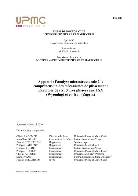
Suppe en 1985 a montré qu‘il existait trois modes majeurs pouvant initier le
plissement des roches (figure 1). (1) Le fléchissement (ou bending) qui apparaît en réponse à
une sollicitation sub-orthogonale aux couches. (2) Le flambage (ou buckling), lié à
Etat des connaissances sur les méthodes appliquées à l’étude du plissement
.

30
Chapitre I
l‘application d'une force d'une manière parallèle aux couches. (3) L‘amplification passive qui
donne une distorsion des plis préexistants causée par un fluage général de la roche. Le
domaine d'application de ce type de mécanisme concerne surtout la déformation des roches
dans le domaine ductile.
Figure 1: Les trois principaux mécanismes de plissement dans les roches (d‘après Suppe, 1985); (1)
le fléchissement (ou bending), (2) le flambage (ou buckling), (3) l‘amplification passive où l‘on assiste
à la distorsion de plis préexistants due au fluage de la roche.
1.3 Classification géométrique des plis
La description précise de la géométrie des plis est un important critère de leur
classification et est considérée comme indispensable à la compréhension du mécanisme de
plissement. Il existe plusieurs classifications géométriques pour les plis. Van Hise en 1894 a
tout d‘abord utilisé le terme de plis semblables et parallèles comme base de classification et
aussi d'implication mécanique des plis. En utilisant le concept de pendage des isogones
(Elliottt, 1965) et les paramètres d'épaisseur (Ramsay, 1962; Zagorcev, 1993), plusieurs
classes ont été introduites pour distinguer les différents types de plis avec une seule couche.
Puis, d'autres auteurs (Hudleston, 1973; Treagus, 1982; Bastida, 1993) ont proposé une
multitude de paramètres pour aider à mieux classifier les plis. Il faut noter que la méthode de
Ramsay (1967) a été un excellent outil pour étudier l'évolution de la géométrie d'une couche
plissée, de sa charnière jusqu'à sa ligne de courbure dans un pli mono-couche, car en général,
toutes les classifications qui ont suivi sont, d'une façon ou d'une autre, des modifications de
cette classification de Ramsay 1967, jusqu'au schéma proposé par Srivastava et Gairola en
1999, qui est devenu le nouveau schéma de classification des plis multi-couches. Cependant,
Etat des connaissances sur les méthodes appliquées à l’étude du plissement
.

31
Chapitre I
pour cette étude, nous allons surtout nous concentrer sur la classification des plis en
s‘appuyant sur leur relation avec les failles.
1.4 Relation pli-faille
La relation pli-faille a fait l'objet de plusieurs études depuis Willis en 1893, qui avait
proposé une première classification pour distinguer les différents types de chevauchements.
Rich, en 1934, a reconnu les plis de cintrage sur rampe (fault-bend-folds), et plus
tardivement la définition du pli de propagation de rampe (fault-propagation fold) a été
proposée (Dahlstrom,1969; Elliott, 1976). Ce dernier type de pli ne se forme pas seulement
par transport (passif) sur rampe préexistante, mais par une propagation simultanée de la faille.
Ces deux derniers modèles ont reçu une formulation géométrique par une série d'articles
(Suppe, 1983; 1985; Suppe et Medwedeff, 1984; 1990; Jamison, 1987 et Mercier et al., 1996).
En 1991, Erslev a créé un modèle cinématique de plissement par propagation de rampe de
type Trishear, repris et développé plus tard par Hardy et Ford (1997) et Allmendinger (1998).
Ce modèle permet de décrire la déformation engendrée au cours de la propagation de la faille
à son extrémité (Grelaud et al. 2000). L'intérêt de ce modèle est aussi de reproduire de
nombreuses caractéristiques observées dans la nature et au laboratoire, dont la variation
progressive du pendage des couches, l'amincissement ou l'épaississement des couches ou
même de la forme de la charnière (Buil, 2002). D'un point de vue mécanique, Maillot, Leroy
Koyi et d'autres ont par une série de travaux (Maillot et Leroy, 2003; 2006; Maillot et Koyi,
2006; Maillot et al., 2007) étudié la relation pli/rampe en construisant une méthode de
prédiction de l‘évolution des chevauchements et des plis, dans les chaînes de montagnes. En
s‘appuyant sur les théorèmes de l‘analyse limite avec des développements théoriques basés
sur l‘analyse limite, et des développements expérimentaux de maquettes en sable, ils ont
choisi une approche analytique qui consiste à affiner les modèles cinématiques développés par
les géologues de terrain sur la base de l‘équilibre mécanique et de la résistance des roches. Le
résultat le plus important est la friction opérée le long de la rampe qui affecte en premier lieu
la taille, l'épaisseur et la vitesse du toit (hanging-wall). Plus la friction et la pente de la rampe
sont importantes, plus l'épaississement des couches est important et moins grande est la
vitesse de déplacement du bloc sus-jacent.
Etat des connaissances sur les méthodes appliquées à l’étude du plissement
.

32
Chapitre I
1.4.1 Plis forcés ou passifs
Selon Stearns 1978, les plis forcés sont des plis pour lesquels la forme finale est
dominée par la forme d'un élément sous-jacent (faille, rampe ou diapir). Pour former ces plis
dans le cas où l'élément sous-jacent est un bloc faillé, il leur est nécessaire de subir le
mouvement de glissement de la faille sous-jacente, ou remontée de diapir le cas échéant.
Généralement, ce type de pli est géométriquement asymétrique (figure 2).
1.4.1.1 Pli de propagation de rampe
Ce groupe de plis est associé aux failles inverses. Le caractère principal des plis de
propagation de rampe (fault-propagation fold) est que le plissement et la faille évoluent
simultanément. À chaque étape de la propagation de la faille, le glissement est totalement
accommodé par le plissement et le pli se développe en « moulant » la rampe (Thompson,
1981).
Figure 2: Exemples de plis forcés. (a) Pli où le fléchissement des couches supérieures est associé au
rejet d‘une faille normale située dans le socle sous-jacent. (b) Roll-over : pli où la courbure des
couches résulte de leur fléchissement (d‘origine essentiellement gravitaire) au niveau d‘une rampe de
faille normale listrique. (c) Pli où le fléchissement des couches supérieures est associé au rejet d‘une
faille inverse située dans le socle sous-jacent. (d) Anticlinal de rampe associé au rejet d‘un
chevauchement. (e) Bombement hémisphérique se rapportant à la poussée verticale due à une
remontée diapirique.
Etat des connaissances sur les méthodes appliquées à l’étude du plissement
.

33
Chapitre I
1.4.1.2 Pli de cintrage sur rampe
Dans ce type de plissement forcé, le plissement ne résulte pas d'un mouvement de
blocs rigides de socle autour d'une faille mais plutôt du mouvement de la faille au sein même
des couches de couvertures. Ils sont généralement formés quand les couches passent du plat à
la rampe, et inversement. La géométrie de ce mode de plissement est clairement différente de
celle des plis de propagation de rampe (fault-propagation fold) (Suppe, 1983; Jamison, 1987
et Mercier et al., 1996). À chaque étape de la propagation de la faille, le glissement est
totalement accommodé par le plissement et le pli se développe en ceinturant la rampe
(Thompson, 1981).
1.4.2 Pli de décollement
Ce mode de plissement, aussi appelé pli de détachement (detachment fold), ne
demande pas l'existence d'une rampe pour se créer, à l'inverse des deux types de plis dits
"forcés". Il se forme au-dessus d'un niveau de décollement comme des évaporites ou de
l'argile, etc… d'où son nom, pli de décollement ou de détachement (figure 3).
Figure 3: Les trois principaux types d'interactions pli/faille (d'après Suppe, 1983 ; 1985 ; Jamison,
1987 et Mercier et al., 1996).
Etat des connaissances sur les méthodes appliquées à l’étude du plissement
.

34
Chapitre I
1.4.3 Conclusion
La différenciation de ces trois types de plis a seulement été basée sur leur géométrie
sans prendre en compte ni considérations cinématiques ni mécaniques. Or, c'est la réponse
mécanique des couches traversées par la faille qui détermine le mode de plissement. Un pli de
détachement serait plus probablement créé quand la faille traverse une couche à
comportement ductile (sel, évaporites, argilites...) (figure 3 c), tandis que, dans le cas de
couches plus compétentes, c'est un pli de propagation de rampe qui serait le plus probable.
Cependant, l'identification du mécanisme responsable de la localisation de la déformation
reste difficile, surtout en ce qui concerne la fracturation liée au plissement (Guiton 2001;
Maillot et Leroy, 2003).
Dans les deux cas de plis de propagation de rampe ou de cintrage sur rampe, les
couches inférieures engagées dans le plissement sont tronquées par la faille. Le pli de
propagation de rampe est associé directement à une rampe ou à une faille sous-jacente, alors
que le pli de cintrage sur rampe se développe ultérieurement par rapport à la formation de la
rampe. La différence se situe surtout au niveau du compartiment supérieur vis-à-vis de la
rampe dans chacun des deux modes. Le pli de propagation de rampe se développe
simultanément avec la propagation de la rampe. Le déplacement tout au long de cette dernière
diminue jusqu'à s'annuler complètement à son extrémité.
Les trois types de plis connaissent trois phases au cours du plissement. La première, le
pré-plissement, correspond au raccourcissement parallèle aux couches (LPS) qui peut
accommoder entre 10 et 30% du raccourcissement total au niveau de certaines chaînes
plissées selon Mitra (1994) et 15% selon Koyi et al. (2003). La deuxième phase du plissement
proprement dite se divise en deux périodes : une correspond à la formation du pli
macroscopique, pendant laquelle la déformation est surtout localisée au niveau de la charnière
et tout le long de la faille si le pli y est relié, et une seconde se rapportant à une période de
serrage tardi-plissement (late stage fold tightening). Ce sont les mécanismes de
microdéformation en relation avec cette phase qui sont les moins connus et que nous avons
tenté d'étudier au cours de cette thèse. La dernière phase, le post-plissement, correspond au
relâchement des contraintes et l'exhumation du pli.
Etat des connaissances sur les méthodes appliquées à l’étude du plissement
.

35
Chapitre I
2 Les mécanismes impliqués dans la
déformation à différentes échelles
A l'échelle des grains, les principaux mécanismes de déformation irréversibles des
roches à l'échelle microscopique efficaces à basse température (

36
Chapitre I
A l'échelle du bassin (figure 4), des études récentes permettent de décrire l'évolution
d'une roche depuis l'avant-pays jusqu‘à son incorporation dans un pli (Roure et al., 2005).
Figure 4: Des blocs diagrammes présentant le développement des structures de deformation comme
les BPS (Bedding parallel shortening), les LPS (layer parallel shortening), les fractures conjuguées et
les fractures hydroliques dans un reservoir carbonate, en relation avec l‘évolution des chaînes d‘avantpays
(d‘après Roure et al., 2005).
Etat des connaissances sur les méthodes appliquées à l’étude du plissement
.

37
Chapitre I
Ces études permettent de montrer où et pourquoi la compaction due à la charge
sédimentaire, la compaction tectonique, la fracturation hydraulique et la fracturation liée à
l'exhumation contemporaine du plissement se succèdent au cours de l'évolution du bassin. A
l'échelle du pli, si plus de travaux relatifs à la répartition spatiale des mécanismes
macroscopiques (failles et fractures principalement) sont disponibles (Guiton et al., 2003 ;
Florez-Nino et al., 2005 ; Bellahsen et al., 2006a ; Ahmadhadi et al., 2007, Wennberg et al.,
2007 par exemple), seules quelques travaux sont bien documentées en ce qui concerne les
microstructures (Frizon de Lamotte et al., 1997 ; Saint-Bezar et al., 2002 ; Louis, 2003 ;
Evans et al., 2003). Il reste alors quelques zones d‘ombres sur l‘évolution mécanique des plis
et les mécanismes qui la contrôlent. De nouvelles observations sur des structures naturelles
dont la géométrie peut être bien définie sont nécessaires.
3 La relation entre le plissement sa courbure et
la distribution de la microdéformation et des
microstructures
Les différents modèles cinématiques des plis sont en général associés à la distribution
de la déformation dans les différentes parties du pli, qui dépend des modes de plissement. Ces
dernières années, et ce grâce au développement de ces modèles cinématiques, plusieurs
tentatives ont été réalisées pour relier la microdéformation ainsi que la fracturation à la
cinématique des plis, au lieu de simplement regarder la forme finale du pli ; cette approche se
justifie par le fait que les microstructures enregistrent une déformation progressive durant le
plissement quand elle lui est contemporaine (Allmendinger, 1982; Bahat 1988 ; Couzens et
Dunne, 1994; Fischer et Anastasio, 1994; Anastasio et al., 1997; Hennings et., al., 2000 ;
Storti et Salvini, 2001; Craddock et Relle, 2003 ; Tavani et al., 2006; Bellahsen et al., 2006) et
influence cette déformation quand elle lui est antérieure (Arlegui-Crespo et Simon-Gomez,
1993; Rawnsley et al., 1998; Ahmadhadi et al., 2008). Cette influence s‘exerce quand la
disposition du ou des familles de veines préexistantes est favorable à leur réactivation et de ce
fait à une perturbation des contraintes lors du plissement.
De nombreuses études ont tenté d'établir un lien entre la macro-déformation
(plissement) et la déformation matricielle ou la déformation interne des couches plissées
(Elliottt, 1976; Engelder et Geiser, 1979; Geiser, 1988; Mitra, 1994; Aubourg et al., 1997;
Louis et al., 2004; Smith et al., 2005), mais aussi d‘étudier la cinématique des plis forcés (en
Etat des connaissances sur les méthodes appliquées à l’étude du plissement
.

38
Chapitre I
relation avec des failles). Parmi les outils employés (qui sont détaillés plus loin dans ce
mémoire), on peut citer à titre d'exemple l'ASM. C‘est un outil efficace pour contraindre les
modifications matricielles des roches comme le raccourcissement parallèle aux couches (LPS)
(Averbuch et al., 1992; Hirt et al., 1995; Frizon de Lamotte et al., 1997; Grelaud et al., 2000)
ou le cisaillement simple (Aubourg et al., 1991). L'ASM reflète fidèlement les orientations
préférentielles des grains et/ou des minéraux qui contribuent à la susceptibilité magnétique
mesurée (Borradaile, 1988; Rochette et al., 1992).
La figure 5 représente un exemple d'étude qui résume la déformation interne associée
à un pli de propagation de rampe selon Saint-Bezar et al. (2002). Selon cette étude, la
déformation peut être accommodée par du glissement flexural comme du cisaillement banc-
sur-banc, et/ou de la déformation interne. Dans les deux cas, le sens de cisaillement est
imposé par le modèle de plissement choisi. Cet exemple comme tant d'autres (dont les plus
récents sont Latta et Anastasio, 2007; Robion et al., 2007; Hnat et al., 2008; Burmeister et al.,
2009; Oliva-Urcia et al., 2009; Amrouch et al., 2010 a et b) montrent à quel point les analyses
de la déformation interne des couches et des microstructures peuvent être discriminantes vis-
à-vis de tel ou tel type de mécanisme de plissement.
Figure 5: Illustration d'un pli de propagation avec la localisation de la zone de cisaillement. La
déformation associée au plissement peut être accommodée par un glissement flexural ou une
déformation interne. La fabrique magnétique due à cette déformation interne est montrée au niveau du
flanc avant du pli (d'après Saint-Bezar et al., 2002).
D'autres études comme celles de Tavani et al. (2006) ont abordé le problème de la
distribution des micro- et mésostructures, ainsi que la relation de cette distribution avec le
plissement et les compartiments du pli. D‘un point de vue quantitatif, les résultats de ces
Etat des connaissances sur les méthodes appliquées à l’étude du plissement
.

39
Chapitre I
travaux ont montré que le plissement est accompagné par le développement de plans
stylolitiques longitudinaux auxquels des joints et des veines sont perpendiculaires. Il a été
montré aussi que l'espacement des principaux plans stylolitiques est lié à l'épaisseur des
couches correspondantes.
Figure 6: Illustration spatiale de la distribution des micro et méso-structures dans un pli asymétrique
(Tavani et al., 2006).
Cette sensibilité à l'épaisseur des couches est analogue à celle décrite dans les
structures ductiles, malgré la différence d‘origine. Les plans stylolitiques montrent une
distribution spatiale qui est liée à leur position dans le pli. Les veines et les joints ne montrent
pas un tel comportement. D'après Tavani et al. (2006), les stylolites sont les structures les plus
appropriées pour déduire la cinématique d'un pli, en utilisant leur fréquence normalisée
(rapport H/S; H étant l'épaisseur de la couche et S l'espacement moyen entre les plans
stylolitiques) et l'angle du plan par rapport à la stratification (ATB). Les différents
compartiments du pli (figure 6), l'avant du pli, le flanc avant (forelimb) et le flanc arrière
(backlimb) et la charnière présentent une distribution spatiale différente de ces deux
paramètres.
En ce qui concerne la fracturation plusieurs études ont tenté de relier le développement
des structures cassantes aux éléments géométriques du pli, comme son axe, ses deux flancs
Etat des connaissances sur les méthodes appliquées à l’étude du plissement
.

40
Chapitre I
avant et arrière et les terminaisons (McQuillan, 1974; Srivastava et Engelder, 1990; Cooper,
1992; Fischer et al., 1992; Erslev et Mayborn, 1997; Jamison, 1997; Thorbjornsen et Dunne,
1997; Hennings, 2000). L'étude publiée par Stearns en 1972 peut être considérée comme une
synthèse du travail pionnier réalisé sur ce thème. Cette synthèse est présentée dans une forme
de classification des fractures (incluant joints et failles) basée sur leur position par rapport aux
caractèristiques géométriques du pli. Ce fameux schéma de population de fractures dans un
anticlinal incluant les fractures axiales, obliques et transversales, était essentiellement statique
et essayait de mettre l'accent sur la relation entre les populations des fractures typiques et leur
localisation dans un pli selon sa forme actuelle. Cette synthèse a ensuite été complétée par une
caractérisation quantitative de la géométrie du pli en utilisant la courbure (Lisle, 2000). La
courbure est encore fréquemment utilisée comme un outil pour définir la direction et la
densité des fractures (Hennings, 2000; Bergbauer et Pollard, 2004).
Keunen et De Sitteren (1938), et Ramberg (1964) après eux ont mis en place un
modèle qui consiste à distinguer deux zones : l‘intrados soumise à une compression locale, et
une zone appelée l‘extrados soumise à une extension locale. La première se distingue par le
développement de stylolites et/ou des failles inverses, et la deuxième présente des fractures de
mode I et probablement des failles normales.
Les travaux de Stearns (1964) puis Stearns et Friedman (1972) ont donné naissance à
un autre modèle plus « complexe » (figure 7) qui résume la distribution des fractures au sein
d‘un anticlinal idéalisé. Dans ce modèle, ils ont essayé d‘expliquer la localisation de chacune
des familles de fractures selon le régime local des contraintes et la situation spatiale dans le
pli. Pour ce modèle, les auteurs ont exprimé trois postulats (pouvant être largement contestés)
qui sont : (a) la totalité des fractures qui peuplent les plis est syn-plissement (ou liée au
plissement), (b) toute fracture oblique à la direction principale de serrage s‘est initiée et
propagée en cisaillement et (c) le régime local des contraintes correspond à celui décrit par le
modèle de Keunen et De Sitteren (1938), et Ramberg (1964).
Les régimes locaux sont sous l‘influence de la contrainte régionale et de la localisation
au sein de la structure plissée (intrados ; extrados ; flanc…).
Dans ce modèle, par leur nombre et leur développement, les ensembles (1) et (2)
semblent prendre les premiers rôles dans l‘évolution du plissement. D‘après ce modèle les
Etat des connaissances sur les méthodes appliquées à l’étude du plissement
.

41
Chapitre I
fracturres (1) résultent d‘un champ de contraintes qui présente un σ1 perpendiculaire à l‘axe
du pli, un σ2 perpendiculaire aux couches et un σ3 parallèle à l‘axe du pli, et elles sont
présentent à toutes les échelles. Moins développées que les (1), les fractures (2) plutôt
d‘échelle centi à décamétrique, elles seraient le résultat d‘un régime à σ1 parallèle à l‘axe du
pli, un σ3 qui lui est perpendiculaire et un σ2 perpendiculaire aux couches. Constitué de
fractures axiales et de failles normales conjuguées de même direction, l‘ensemble (3) serait la
cause de l‘extension située au niveau de l‘extrados, quand à l‘opposé l‘ensemble (4) traduit
par ces failles inverses le régime compressif à l‘intrados. Le dernier ensemble exprimé dans
ce modèle (5) est rencontré au niveau des interfaces des bancs. Il est représenté par des failles
normales conjuguées au plan de glissement entre bancs.
Figure 7: Modèle classique de distribution des fractures au sein d‘un anticlinal idéalisé inspiré du
Teton Anticline, Montana, U. S. A. (d‘après Stearns, 1964, et Stearns et Friedman, 1972)
Comme on l‘a exprimé précédemment, les postulats sur lesquels se base ce modèle
restent contestables. En effet, plusieurs études ont montré l‘influence que pourraient avoir des
fractures préexistantes sur le plissement et la fracturation qui lui est associée (Arlegui-Crespo
et Simon-Gomez., 1993; Rawnsley et al., 1998 ; Bergbauer et Pollard, 2004 ; Bellahsen et al.,
2006 ; Ahmadhadi et al., 2008). La réactivation de ces fractures préexistantes agit
essentiellement sur les contraintes à la fois par un relâchement de ces dernières et par une
réorientation de leurs directions, cette variation de l‘état de contrainte peut avoir comme effet
d‘inhiber ou favoriser la formation de certaines familles de fractures. L‘utilisation de
méthodes d‘analyses comme celle des macles de la calcite ou celle des propriétés
petrophysiques des roches permettrait de scruter l‘évolution des contraintes et de la
microdéformation pendant le plissement.
Etat des connaissances sur les méthodes appliquées à l’étude du plissement
.

43
Chapitre II
Chapitre II : LES METHODES D'ANALYSES
DE LA MICRODEFORMATION : MACLES
DE LA CALCITE ET PROPRIETES
MAGNETIQUES ET PHYSIQUES DES
ROCHES
Les méthodes d’analyses de la microdéformation
.

45
Chapitre II
1 L'analyse des macles de la calcite
1.1 Introduction
La déformation par maclage des cristaux de calcite est caractéristique du régime de
transition cassant-ductile dans la partie supérieure de la croûte. Elle fait partie des différents
mécanismes de déformation qui accompagnent la déformation cassante des roches, comme la
pression-dissolution (Durney, 1972 ; 1976; Rutter, 1976 et Gratier, 1984) et la réduction de la
porosité (Carrio-Schaffhauser et Gaviglio, 1990). Le maclage e [10 12] est plus facilement
activé que les autres systèmes de glissement dans le domaine de basse température (0-300°)
dans la calcite, ce qui explique sa dominance dans ces conditions. Depuis 1953, grâce à
Turner, nous savons que les macles de la calcite peuvent être utilisées pour déterminer
l'orientation des contraintes principales responsables de la déformation cristalline observée.
Chaque cristal de calcite présente trois familles de plans de macle potentiels. Ce sont les
mesures d‘inclinaison et de direction de ces plans maclés, de leur épaisseur et de leur densité
qui permettent de remonter selon la méthode utilisée, soit au tenseur de déformation
(Groshong, 1972) soit au tenseur de contrainte (Etchecopar, 1984).
1.2 Analyse de la contrainte et de la déformation par le
maclage
Le maclage e de la calcite est utilisé par plusieurs méthodes d'analyse pour déterminer
l'état des contraintes et l'état de déformation finie subis par la roche (Groshong, 1972 ; 1974;
Laurent et al., 1981 ; Laurent, 1984; Etchecopar, 1984; Pfiffner et Burkhard, 1987 ; Laurent et
al., 1990 et Lacombe, 2001). Ces méthodes reposent toutes sur l'hypothèse selon laquelle les
macles se sont formées dans un champ de contrainte homogène et que l'échantillon n'a pas
subi de rotation relative au champ de contrainte au cours de sa déformation. Le
développement des macles de la calcite dépendant peu de la température (sauf en ce qui
concerne leur allure –fines ou épaisse)s, ni (ou très peu) de la vitesse de déformation, ni même
de la pression de confinement, il apparaît comme un bon paléopiézomètre (Spiers, 1979).
Comme résumé par Lacombe (1992), les travaux expérimentaux sur des roches calcitiques ont
permis de préciser la contribution du maclage à la déformation basse-température des roches
carbonatées (Spiers, 1979 ; Wenk et al., 1986 et Schmid et al., 1987):
Les méthodes d’analyses de la microdéformation
.

46
Chapitre II
Les macles s'initient à des stades précoces de la déformation, et leur développement
dépend essentiellement de l'orientation des cristaux par rapport au champ de
contraintes appliqué;
C'est l'intensité de la contrainte différentielle et la taille des grains qui contrôlent
l'apparition des macles;
La déformation par maclage se distribue de façon très hétérogène à l'échelle du grain,
et ne reflète pas la déformation totale imposée à la roche. Au contraire, l'orientation de
la contrainte est beaucoup plus homogène à l'échelle du grain (15° de déviation en
moyenne par rapport à la contrainte appliquée) (Spiers, 1979);
Dans les cristaux bien orientés pour macler, la densité de maclage et la largeur des
macles sont directement liées à la déformation subie par ces cristaux. A basse
température, l'augmentation de la déformation produit préférentiellement de nouvelles
macles fines (Groshong, 1974);
Le maclage intervient seulement dans une fraction de la déformation totale, et les
phénomènes de pression-dissolution à basse température, ou les glissements
intracristallins à haute température (glissement r ou f), aident à maintenir la
compatibilité géométrique de la déformation des grains adjacents.
Les méthodes d'inversion disponibles sont capables, à partir de l'observation des plans
maclés et non-maclés des cristaux de calcite présents dans un échantillon, de calculer
l'orientation des axes du tenseur de contrainte responsable du maclage, son rapport de forme
et les contraintes différentielles associées. Pour déterminer le tenseur complet, il reste à
déterminer la composante isotrope du tenseur. Il est donc nécessaire d'utiliser une approche
complémentaire telle que l‘étude de la fracturation, combinée aux propriétés mécaniques des
roches étudiées, l'analyse des inclusions fluides, l‘estimation de l'enfouissement des roches
que l'on étudie (Lacombe et Laurent, 1992; Lacombe, 2001).
L'étude des macles de la calcite apparaît donc comme un outil puissant pour contrôler
l'évolution des contraintes au cours de la formation d'un pli. On notera que les macles de la
calcite permettent également de déterminer dans les sites polyphasés plusieurs tenseurs dont
les directions principales sont corrélables à celles déterminées indépendamment et au même
endroit par l'analyse des jeux de failles (Lacombe et al., 1990). Les résultats de l'analyse des
macles dans les échantillons polyphasés sont significatifs, à la fois d'un point de vue
numérique (solutions stables) et géologique. L‘analyse des macles de la calcite apparaît donc
complémentaire de l‘étude de la fracturation macroscopique ; quoique reposant sur des
principes semblables (analogie géométrique faille/macle, principe de l'inversion), ces deux
méthodes analysent des déformations très différentes, en particulier du point de vue de leur
genèse (mécanique de la rupture versus dislocation intracristalline) et de leur échelle. Ainsi,
par exemple, les roches carbonatées peuvent enregistrer par maclage des événements
Les méthodes d’analyses de la microdéformation
.

47
Chapitre II
tectoniques "mineurs", au cours desquels la montée en contrainte n'a pas été suffisante pour
provoquer la rupture macroscopique, et qu'inversement (mais plus rarement), des failles
peuvent être observées dans un site dans lequel le tenseur correspondant n'est pas identifiable
par l'analyse des macles. Ces enregistrements différentiels des paléo-champs de contraintes
dénotent une sensibilité différente de ces mécanismes de déformation à la contrainte. Les
deux méthodes offrent également des possibilités différentes lors de l‘acquisition des données
ou de l'exploitation des résultats. Ainsi, seule l'analyse des macles de la calcite permet de
reconstituer les directions de paléocontraintes à partir de quelques cm3 d'échantillon prélevé
par exemple en forages; en contrepartie, en contexte polyphasé, les données de fracturation
permettent généralement plus facilement l‘établissement en routine d'une chronologie relative.
L‘un des objectifs de cette thèse est de combiner les données de ces différentes approches afin
d‘établir une histoire tectonique plus complète des structures géologiques, et d‘aller plus loin
dans la détermination des magnitudes des contraintes en 4D (à l‘échelle d‘une structure
géologique et au cours du temps).
1.2.1 Définition des macles
1.2.1.1 Caractéristiques du maclage
Une macle est définie comme une association polycristalline, formée par la
juxtaposition de deux parties homogènes ou plus. Ces dernières sont orientées l'une par
rapport à l'autre, suivant des lois bien définies. Le maclage est manifestation de la migration
d‘une dislocation coin le long du plan de glissement (plan de macle) (figure 8). Si le cristal
n'est traversé que par un plan de composition, la macle est dite simple. Le plan de macle est
un plan de densité atomique importante qui sépare le domaine maclé relatif au cristal-hôte du
domaine non maclé (dans le cristal de calcite le plan de macle est parallèle à un plan de
composition [01 1 2]). Si la loi de macle est répétée dans le même cristal, la macle est dite
multiple ou polysynthétique. Si l'on considère qu'une macle est un petit domaine de
cisaillement simple, le plan de macle, qui est le plan atomique commun aux deux parties de la
macle, serait l'équivalent géométrique du plan de cisaillement.
La direction de maclage est définie comme la droite qui lie la position d'un atome
donné avant le maclage et d‘un atome après le glissement et correspond donc à la direction de
glissement. Cette direction appartient au plan de macle et correspond à la projection de l'axe
Les méthodes d’analyses de la microdéformation
.

48
Chapitre II
optique sur ce plan. Elle coïncide également avec l'intersection du plan de macle e1 et des
plans de clivage r2 ou r3.
1.2.1.2 Géométrie du maclage e de la calcite
Chaque cristal possède trois familles de plans de macle e potentiels [01 1 2] qui sont
disposées symétriquement par rapport à l'axe optique (axe de symétrie ternaire : figure 9).
Figure 8: Présentation schématique du processus de maclage.
Le maclage est géométriquement comparable à un microcisaillement, dont la direction
et le sens sont imposés par le cristal hôte. Si on le compare à un jeu de failles, tout se passe
comme si le plan de faille préexistait et la strie réelle était imposée. Le sens de maclage e
[défini comme positif par Turner et al. (1954)] est tel que l'axe optique étant vertical, le
déplacement relatif des atomes situés au-dessus du plan de macle s'effectue, vers l'axe optique
en mouvement en "faille inverse" (du bas vers le haut).
Une lamelle de macle est géométriquement analogue à un micro-couloir de
cisaillement ; elle correspond à la portion de cristal maclée située entre deux plans de macle e
dans laquelle les atomes n'ont pas la même orientation que dans la portion non maclée du
cristal-hôte.
Les méthodes d’analyses de la microdéformation
.

49
Chapitre II
Figure 9: Projection stéréographique des pôles des plans de macle e, de clivage r et de l'axe optique C
(Turner et Weiss, 1976).
1.2.1.3 Initiation et développement des macles
Le maclage se produit si la contrainte cisaillante appliquée dans la direction et le sens
de maclage est suffisamment forte pour macler. On aura donc là une indication qualitative et
quantitative précieuse à tirer de l'étude des plans maclés et non maclés.
La contrainte cisaillante résolue critique (CCRC) ou seuil de maclage a est la valeur
de la contrainte qui doit s‘appliquer dans la direction et le sens de maclage pour que celui-ci
ait lieu.
La valeur CCRC est obtenue par la relation :
a = * S
Avec la valeur de la contrainte appliquée au point critique (sur la courbe /) et S le
facteur de Schmid, tel que S:
Les méthodes d’analyses de la microdéformation
.

50
Chapitre II
S = cos * cos
: Angle entre la direction de compression et la normale au plan de macle dans un
monocristal; : angle entre la direction de compression et le vecteur déplacement par
maclage.
La valeur du seuil de maclage est largement indépendante de la température, de la
pression de fluide et de la pression isostatique. Elle dépend surtout de la taille des grains et de
la distribution de celle-ci (Newman, 1994), mais aussi de la déformation interne qui cause le
durcissement du grain (Laurent et al., 2000). La valeur de 10 MPa est habituellement utilisée
pour les grains dont la taille moyenne se situe entre 300–400 µm (Turner et al., 1954; Laurent,
1984; Lacombe et Laurent, 1996).
Cette valeur du seuil, après différents travaux expérimentaux, a été estimée
initialement à 10 MPa, mais elle doit être adaptée à la taille des grains et au pourcentage de
déformation (Lacombe, 2001). Laurent et al. (2000) ont démontré que le seuil de maclage
dépend fortement de la déformation interne (causée par le strain hardening), et fluctue entre 5
et 7 MPa pour les zones faiblement déformées (~ 1% de déformation) jusqu'à 13–15 MPa
dans les zones moyennement déformées (vers 4% de déformation).
Pour qu‘un plan d‘orientation donnée par rapport aux axes de contraintes macle la
contrainte cisaillante résolue doit dépasser le seuil supposé constant de maclage ; même si
celle-ci augmente, le plan ne maclera pas " davantage" pour autant (loi du tout ou rien).
1.2.2 Les facteurs qui influent sur le maclage et son seuil
1.2.2.1 Rôle de la contrainte différentielle
Les données expérimentales montrent que pour une taille de grain, une température et
une pression de confinement données, la contrainte différentielle (1-3) est l‘un des facteurs
qui influence le plus le nombre de macles par millimètre dans un cristal (twin density), le
pourcentage de la fraction maclée du cristal (twin volume fraction) et le pourcentage de
cristaux maclés dans un agrégat (twinning incidence). Il faut noter que la formation d'une
macle mécanique est un processus discontinu à toutes les échelles. L'initiation d'un micro-
élément maclé demande des contraintes plus élevées que le développement et la propagation
ultérieurs de la macle, à partir de ce micro-élément. Il est aussi important de souligner que la
Les méthodes d’analyses de la microdéformation
.

51
Chapitre II
contrainte différentielle seuil correspond à la contrainte nécessaire à la propagation de la
macle, quand celle-ci est déjà initiée. En effet, les macles mécaniques s'initient probablement
en des zones de concentration de contraintes, telles que les discontinuités mécaniques (joints
de grain, points triples, etc) nombreuses dans les cristaux et agrégats naturels.
1.2.2.2 Rôle de la température
La température a un rôle important sur l'allure des macles et non sur leur
développement, car ce n'est pas un mécanisme thermo-activé.
Par contre, la densité de maclage en dépend car au cours de la déformation, il est plus
facile de créer de nouvelles macles que d‘épaissir les macles existantes à température
inférieure à 170-200°C. La déformation par cisaillement simple est alors absorbée par de
nombreuses macles très fines, donc la densité de maclage augmente suivant la flèche bleue
(figure 10). Inversement, à température supérieure à 200°C, il est plus facile d‘épaissir les
macles que d‘en créer de nouvelles : on obtient des macles qui sont moins nombreuses mais
très épaisses. La déformation se fait donc suivant la flèche orange (figure 10), à température
supérieure à 200°C, et se fait suivant la flèche bleue à température inférieure à 170°C. La
largeur des macles et la densité de maclage sont alors utilisables comme des indicateurs de la
température associée à la déformation naturelle des calcaires (Ferrill, 1998 ; Ferrill et al.,
2004), bien qu‘une étude récente vienne nuancer ces résultats (Janssen et al., 2007).
Figure 10: Graphique de l'intensité moyenne de macles versus l'épaisseur moyenne des plans de
macle. Les couleurs sont en relation avec le degré de déformation. Les flèches orange et bleue
illustrent respectivement le sens d'augmentation de la déformation pour 200° et 170°. D‘après Ferrill et
al. (2004).
.
Les méthodes d’analyses de la microdéformation

52
Chapitre II
L'épaisseur moyenne des macles de la calcite est directement corrélée à la température
de déformation, de sorte que les macles fines sont dominantes à une température inférieure à
170°C et à ce que les macles épaisses dominent pour les températures supérieures à 200°C.
Au-delà de 250°C, la recristallisation dynamique devient un important mécanisme. La densité
de maclage (nombre de plans de macles/mm) se corrèle inversement à la température, et la
combinaison de données d'intensité de maclage avec l'épaisseur des macles peut donner des
informations tant sur l'intensité que sur la température de la déformation. Cette relation fournit
un géothermomètre (BT) de déformations pour les roches qui présentent peu ou pas de
données de paléotempérature.
1.2.2.3 Rôle de la vitesse de déformation
La "twinning incidence", la "twin volume fraction" et le nombre de macles par mm
("twin density") sont à peu près indépendants à la vitesse de déformation (Friedman et Heard,
1974; Tullis, 1980 ; Rowe et Rutter, 1990).
Les méthodes d’analyses de la microdéformation
.

53
Chapitre II
Figure 11: Graphiques des caractéristiques du maclage, à partir d'échantillons des Alpes et
Appalaches. Les codes de couleur sont en fonction de la température de déformation déduite du
maximum d'enfouissement ou des indicateurs métamorphiques. (a) Épaisseur moyenne des macles
versus déformation par maclage, (b) densité de maclage versus déformation par maclage, (c) densité
de maclage versus épaisseur moyenne des macles, (d) produit de l'épaisseur moyenne des macles et de
densité de maclage (rapport cristaux maclés par cristaux non maclés) versus la déformation par
maclage. Points incluant des données du tableau 1 de Ferrill (1991), Spraggins et Dunne (2002;
données brutes), et Smart et al. (1997; données brutes). Des données microthermométriques non
publiées d'inclusions fluides de M.A. Evans ont été utilisées pour contraindre les 65°C, la température
des échantillons de Smart et al. (1997) et la température de 235°C définie à partir des données d'Evans
et Dunne (1991). Les lignes rouges et bleues séparent les domaines de données caractérisées par la
déformation à la température de 170, 170–200, et 200 °C. D‘après Ferrill et al. (2004).
Les méthodes d’analyses de la microdéformation
.

54
Chapitre II
Figure 12: (a) Illustration schématique de l'influence de la température sur la déformation par maclage
de la calcite (d'après Burkhard, 1993). Exemples de photos des différents types de macles (lumière
polarisée). (b) Macles de type I de la Chaîne Subalpine du nord, France (Ferrill, 1991). La largeur de
la photo est de 0.68 mm. (c) Macles de type II du Nord de Mountain thrust sheet dans la Great Valley,
Central Appalachian Valley et Ridge Province (Evans et Dunne, 1991). À noter que les macles fines
sont localement développées avec les macles épaisses. La largeur de la photo est de 0.22 mm. (d)
Macles de type III des Ardon thrust slice des Diablerets nappe dans les Alpes Helvétiques (Burkhard,
1990). La largeur de la photo est de 0.14 mm. (e) Macles de type IV des Doldenhorn nappe
(échantillons 199.3) dans les Alpes Helvétiques (Burkhard, 1990). La largeur de la photo est de 0.14
mm. Les photos (d) et (e) sont prises à partir de lames ultra-fines (épaisseur approximative de 5
microns ou moins).
1.2.2.4 Rôle la pression isotrope et de la pression de fluide
Turner et al. (1954) ont montré que la contrainte normale sur un plan de macle donné
augmente la contrainte cisaillante critique nécessaire au maclage de moins de 1% de la valeur
de cette contrainte normale. Friedman et Heard (1974) confirment que les macles
n‘apparaissent pas si l‘échantillon est soumis uniquement à une pression isotrope.
Les méthodes d’analyses de la microdéformation
.

55
Chapitre II
1.2.2.5 Rôle de la taille des grains
La limite des cristaux est un frein au développement des macles qui se propagent dans
le cristal comme une fracture en mode de cisaillement. Au cours de plusieurs études
expérimentales, Schmid et Paterson (1977), Casey et al. (1978), Spiers (1982) et Spiers et
Rutter (1984) ont montré qu'il est plus facile de macler les cristaux de grande taille que ceux
de petite taille. Ainsi, plus les cristaux de calcite sont gros, plus il est facile de développer des
macles. Pour une même contrainte différentielle, plus la taille des grains est importante, plus
le pourcentage de macles est grand (figure 13). Ce constat est dû au rapport entre le bord des
grains et le volume des grains, paramètre qui influe sur le maclage. Lorsque la taille des
grains augmente, le seuil du maclage diminue. Il faut donc prendre en compte l‘influence de
la taille du grain lors de l'application des méthodes inverses, qui présupposent une valeur
constante du seuil de maclage.
1.2.2.6 Rôle de la déformation interne
Plusieurs études expérimentales ont montré qu'il est plus facile de macler des cristaux
non déformés que de reprendre des cristaux déjà maclés (phénomène de "strain hardening").
Ainsi, plus les cristaux sont déformés, plus il est difficile d‘y développer de nouvelles macles.
On notera qu‘à plus haute température ou lorsqu‘une roche subit trop de déformation que le
maclage seul ne peut absorber, d‘autres mécanismes prennent le relai (glissement sur les plans
de clivage), entraînant parfois une allure courbe de certaines macles.
En admettant que des grains de calcite de différentes tailles ont enregistré la même
contrainte différentielle pour une phase tectonique donnée et au vu de l‘influence de la taille
des grains sur le seuil de maclage, la valeur que l‘on devrait choisir pour ce dernier doit
dépendre de la taille des grains ; Rocher et al. (2004) ont d‘ailleurs pris en compte la variation
de la taille des grains de la calcite dans la désignation du seuil de maclage. En effet sur les
échantillons traités au cours de cette thèse, on a noté que plus la taille des grains est petite,
plus le taux de déformation est faible et ce pour le même échantillon et pour la même phase
tectonique. En se basant sur nos remarques et nos mesures, on a essayé dans la figure 13 de
représenter l‘évolution de la valeur du seuil de maclage par rapport à la taille du grain et aussi
par rapport au taux de déformation. Ces courbes ont été obtenues en se basant sur les données
de macles (Lacombe et al., 2007; Lacombe et al., 2009; Amrouch et al., 2010a). On propose
Les méthodes d’analyses de la microdéformation
.

56
Chapitre II
de détailler l‘exemple de l‘échantillon SMA7 qui présente des cristaux de tailles très
différentes (Figure 13). Après l‘analyse des macles de la calcite pour cet échantillon, on a
décidé de retraiter les cristaux mesurés mais cette fois en les séparant en deux catégories. La
première catégorie présente des grains de calcite dont la taille est supérieure à 300 µm et la
deuxième catégorie regroupe les cristaux dont la taille est inférieure à 300 µm. On a choisi la
taille de 300 µm car c‘est elle qui permettait d‘avoir un nombre à peu près équivalent de
cristaux dans chacun des groupes.
NB : ce raisonnement devient plus compliquer à appliquer dans le cas des cristaux en
fibres vu la grande variation du diamètre du cristal dans l‘espace.
Figure 13: Évolution de la valeur du seuil de maclage en fonction de la taille des grains de calcite. Ces
résultats sont basés sur les différentes données de macles obtenues sur plusieurs échantillons venant du
Fars (Lacombe et al., 2007), d‘Albanie (Lacombe et al., 2009), du Pli de Sheep Mountain (Amrouch et
al., 2010a) et prend en compte aussi les résultats sur la relation seuil de maclage/taille des grains de
Rocher et al. (2004).
Le tableau 1 résume les résultats obtenus par ce traitement. Pour ces deux groupes, on
note une similitude dans les directions des axes principaux des contraintes et souvent pour le
rapport , mais la valeur du seuil interne ‘a (voir p 65-66) est plus faible pour les cristaux de
petite taille, ce qui signifie que pour que ces derniers maclent, ils devraient subir une
contrainte plus élevée. Vu que les deux groupes ont enregistré le même état de contrainte, cela
signifie que le seuil de maclage est plus important pour les petits cristaux. On a aussi noté que
le deuxième tenseur n‘a été enregistré que par les cristaux de grande taille ; les contraintes qui
en sont responsables n‘étaient certainement pas assez fortes pour atteindre le seuil de maclage
Les méthodes d’analyses de la microdéformation
.

57
Chapitre II
des petits cristaux. Si cet état de contrainte est tardif il faut prendre aussi en compte l‘effet du
durcissement des cristaux par le premier événement de maclage, ce qui augmente encore la
valeur de son seuil.
Sur la figure 13, il faut envisager que pour des tailles de cristaux importante (> 700-
800 microns) ou faible (

58
Chapitre II
Figure 14: Photo d‘une veine de calcite de l‘échantillon SMA7 illustrant la différence de taille des
cristaux mesurés dans un même échantillon : en bleu des gros cristaux de calcite maclée et en rouge
des petits cristaux de calcite maclée.
Illustration des différents degrés de déformation obtenus dans les échantillons de Sheep
Mountain.
Le tableau 2 et la figure 15 montrent des exemples de grains de calcite maclée avec
différent pourcentage de déformation (lié directement à la densité de maclage). Les valeurs de
ces pourcentages de déformation ont été calculées en prenant en compte l‘épaisseur moyenne
des macles, le nombre de ces derniers, l‘épaisseur des macles par rapport au diamètre du
grain. Il faut noter que ce taux représente une moyenne pour chaque échantillon, car il faut
Les méthodes d’analyses de la microdéformation
.

59
Chapitre II
faire ce calcul pour chacune des familles de macles quand le grain de calcite en présente plus
d‘une, et le refaire ensuite pour l‘ensemble des grains mesurés.
Figure 15: Exemples de cristaux de calcites maclées avec une densité de maclage qui diminu de
gauche à droite ; on note une différence de densité pour l‘échantillon (1) entre la veine (faible densité)
et la matrice (forte densité de maclage), on peut déduire de cet exemple que le maclage enregistré dans
la veine est postérieur à celui enregistré dans la matrice.
Les méthodes d’analyses de la microdéformation
.

60
Chapitre II
Figure 16: A : valeurs et évolution comparées des seuils de maclage et d‘activation des systèmes de
glissement avec la température (d‘après De Bresser et Spiers, 1997 et Lacombe, 2001).
Avant de commencer l‘aquisition des mesures, on scanne la lame ce qui permet de
localiser et numéroter chacun des cristaux mesurés (figure 17). Ceci rend possible le
traitement des grains par catégorie de taille (quand le nombre de cristaux par catégorie le
permet) et aussi de faire les allées-retours entre les fichiers de traitement et la lame afin de
relocaliser les cristaux en cas de besoin d‘une quelconque vérification.
Les méthodes d’analyses de la microdéformation
.

61
Chapitre II
Figure 17: Photo des veines N-S et S-W de l‘échantillon P37, les cristaux de calcite mesurés sont
numérotés.
1.3 Méthodes de quantification des paléocontraintes et
de la déformation par les macles de la calcite
Depuis l'étude pionnière de Turner (1953), plusieurs méthodes d'analyses de
contraintes ont été développées en se basant sur les données de macles de la calcite (Jamison
and Spang, 1976 ; Laurent et al., 1981 ; Laurent, 1984 ; Etchecopar, 1984 ; Pfiffner and
Burkhard, 1987 ; Laurent et al., 1990 et Nemcok et al., 1999).
Que ce soit pour déterminer les directions ou les grandeurs des contraintes,
l'application du maclage de la calcite dans les problèmes structuraux et tectoniques était
restreinte au début seulement, aux carbonates (Groshong, 1975 ; Engelder, 1979 ; Spang and
Groshong, 1981 ; Wiltschko et al., 1985 et Craddock et al., 1993), aux veines de la calcite
(Kilsdonk et Wiltschko, 1988), ou plus rarement, aux marbres (Craddock et al., 1991). Les
veines et vacuoles de calcite dans les basaltes ont été récemment analysées par ces méthodes
(Craddock and Pearson, 1994; Craddock et al., 1997; Craddock et al., 2004).
Les méthodes d’analyses de la microdéformation
.

62
Chapitre II
L'étude des grandeurs des contraintes dans la croûte est un important thème de
recherche pour les Sciences de la Terre. Mais à ce jour, la connaissance des valeurs des
contraintes que subit la croûte terrestre reste rudimentaire. Les données de magnitude de
contraintes actuelles sont rares et sont essentiellement obtenues dans les régions intraplaques,
où l'état de contrainte est généralement de type décrochant ou compressif : USA, Sud Afrique
(McGarr et Gay, 1978); Scandinavie, Europe centrale (Rummel et al., 1986); Monticello,
Caroline du Sud (Zoback et Hickman, 1982); Angleterre, Cornwall (Pine et al., 1983); Yucca
Mountain, Nevada (Stock et al., 1985); Fenton Hill, Nouveau Mexico (Barton et al., 1988);
Cajon Pass, Californie (Zoback et Healy, 1992; Vernik et Zoback, 1992); Allemagne (Brudy
et al., 1997; Zoback et Harjes, 1997). Le fait de déduire la magnitude des paléocontraintes via
l‘étude du développement des structures géologiques naturelles est difficile (Lacombe, 2001 ;
2007). Un premier type d'approche consiste à combiner l'inversion de données de failles
striées avec les données de la mécanique des roches et/ou la détermination de la pression de
fluide existante pendant la déformation cassante. À ce jour, Bergerat et al. (1985), Angelier
(1989) et Reches et al. (1992) utilisent l'enveloppe de friction et/ou de rupture pour mieux
contraindre le tenseur de contrainte obtenu par l'analyse inverse des données de failles striées.
Lespinasse et Cathelineau (1995) puis André et al. (2002) ont combiné l'inversion des
données de glissement de failles avec les données des inclusions de fluide pour déterminer la
magnitude des contraintes principales. L'approche alternative est basée sur l'étude des
paléopiézomètres, telle que la densité de dislocation dans la calcite (Pfiffner, 1982), la
recristallisation dynamique de la calcite et du quartz (Twiss, 1977; Weathers et al., 1979;
Kohlstedt et Weathers, 1980), et le maclage mécanique dans la calcite et la dolomite (Jamison
et Spang, 1976 ; Rowe et Rutter, 1990 ; Lacombe et Laurent, 1992 et 1996).
Dans la partie qui suit, je vais résumer comment la magnitude de la contrainte
différentielle peut être déterminée en utilisant les macles de la calcite, et aussi comment la
combinaison des données de macles avec les données de fracturation et de la mécanique des
roches peut aider à contraindre le tenseur de contraintes complet (Lacombe et Laurent, 1992 ;
Lacombe, 2001 et 2007).
Les méthodes d’analyses de la microdéformation
.

63
Chapitre II
1.3.1 La détermination du tenseur déviatorique
1.3.1.1 Acquisition des données de macles
Les échantillons sur lesquels les mesures sont effectuées sont orientés dans l‘espace.
Dans ces échantillons, on a taillé au moins trois lames orientées pour chaque échantillon,
selon trois plans orthogonaux.
Dans ces lames, on mesure si possible au moins 30 cristaux par lame, à l‘aide de la
platine universelle (figure 18), en notant la direction par rapport au Nord de la platine, et le
pendage de chaque famille de macles. Un logiciel (Tourneret, 1990) détermine la position
des deux axes optiques possibles à partir de deux plans de macle mesurés sur la base
des relations angulaires et de symétrie entre les plans de clivage, les plans de macle et
l'axe optique.
Figure 18: Platine universelle
L‘axe qui correspond à une extinction totale lors de la rotation suivant l'axe E-W de la
platine est l'axe optique du cristal de calcite. Une fois l'axe optique défini, le programme
informatique nous donne l'orientation des plans de macles manquants. Le caractère maclé ou
non maclé des plans est alors vérifié optiquement et entré dans le programme ainsi qu'un
pourcentage de confiance sur cette détermination. L‘importante différence avec les mesures
de failles est que cette méthode nous permet à la fois d‘utiliser les plans maclés comme les
plans non maclés. Ces derniers ne peuvent pas être mesurés directement, car on ne voit rien
Les méthodes d’analyses de la microdéformation
.

64
Chapitre II
(pas de lamelle de macle). Cependant, on peut indirectement mesurer leurs directions et leurs
pendages. Ces plans non maclés sont importants pour calculer les orientations et les grandeurs
des contraintes, car si ces plans-là n‘ont pas maclé cela signifie que soit la direction et le sens
de la contrainte exercée n‘étaient pas compatibles avec le sens de maclage soit que le seuil de
la maclage n‘était pas atteint (figure 19).
Une fois tous les axes optiques déterminés pour les cristaux de chaque lame, on
calcule les rotations qu‘il est nécessaire d‘appliquer à chaque lame, afin de remettre les
données correspondantes par rapport au Nord géographique.
Chaque fichier contenant les données des trois lames d‘un échantillon est traité en
utilisant le programme d‘inversion d‘Etchecopar (1984), pour définir un tenseur qui rend
compte d‘un certain pourcentage (le plus grand possible) de plans maclés et la totalité des
plans non maclés. Ce pourcentage est optimisé par l‘utilisateur sur la base de la stabilité de la
solution (voir exemple de traitement d‘échantillon).
Pour vérifier si un échantillon a connu un polyphasage, on peut grâce au même
programme, déterminer le deuxième ou même le troisième tenseur responsable de ces
différentes phases. Cela se fait en traitant les plans maclés non expliqués par le premier
tenseur, et la totalité des plans non maclés, données contraignantes, mais malheureusement en
nombre décroissant en cas de polyphasage.
Cette technique d'inversion est jusqu'à aujourd'hui la seule technique qui permet de
calculer simultanément les orientations des contraintes principales ainsi que la contrainte
différentielle à partir de données de calcite d'un même échantillon. Par conséquent, cela
permet de relier dans un régime de contrainte, la magnitude de la contrainte différentielle à
l'orientation d'une contrainte donnée, malgré certaines limitations (Gagala, 2009). De
nombreuses études ont pu démontrer le potentiel de cette méthode pour décrire l'histoire
tectonique régionale ou locale qu‘elle soit mono- ou polyphasée (Lacombe et al., 1990 ;
1993 ; 1996 ; 2007 ; Rocher et al., 1996 ; 2000 et Amrouch et al., 2010a).
NB : il faut noter que la platine universelle présente quelque limite concernant les
mesures, vu que les plans qui présentent un pendage supérieur à 55° sont difficiles à mesurer.
Il arrive que l‘on ne puisse pas voir si le plan est maclé ou pas. C‘est pour cette raison que
Les méthodes d’analyses de la microdéformation
.

65
Chapitre II
dans le programme utilisé, on donne à chaque fois un pourcentage de confiance au caractère
maclé ou non maclé d‘un plan ; l‘utilisation de 3 lames minces perpendiculaires permet de
résoudre en grande partie le problème de la couverture spatiale des orientations des axes
optiques et des plans de macles.
1.3.1.2 Traitement des données : détermination des orientations
de paléocontraintes
L'hypothèse de base de l'analyse tectonique du maclage e est qu'il se produit sur un
plan e donné si et seulement si la contrainte cisaillante résolue s sur le plan e est supérieure
ou égale à la valeur critique, supposée constante, du seuil de maclage a. Ainsi, pour les plans
maclés : s ≥ a et pour les plans non maclés : s < a. Le principe de l'analyse inverse
(Etchecopar, 1984) est de déterminer le tenseur (ou les tenseurs si l'échantillon est polyphasé)
qui vérifie(nt) les inéquations ci-dessus pour un pourcentage maximal de plans maclés et pour
la totalité des plans non maclés. Les plans non maclés exercent une forte "contrainte" sur la
détermination des tenseurs, car la contrainte cisaillante résolue (CCR) induite sur ces plans
non maclés doit toujours rester inférieure au seuil (figure 19).
Figure 19: Illustration des domaines des plans maclés et plans non maclés.
La solution est recherchée sous la forme d'un tenseur réduit, avec une contrainte
différentielle (l - 3) normalisée à 1. La CCR s qui s'exerce sur chaque plan de macle varie
alors dans l'intervalle (-0,5; +0,5). La première étape consiste à choisir arbitrairement un
pourcentage P de plans maclés à expliquer. Un grand nombre de tenseurs sont alors tirés au
hasard puis appliqués au lot de données. Les CCR s sont calculées pour tous les plans de
macle qui sont classés par ordre de CCR décroissante. Cette classification permet d'évaluer
rapidement si le tenseur recherché induit sur certains plans non maclés une CCR plus grande
Les méthodes d’analyses de la microdéformation
.

66
Chapitre II
que celle qui s'exerce sur certains plans maclés expliqués par ce tenseur, c‘est-à-dire le
nombre de plans non maclés incompatibles avec la solution. Le cas idéal, rare en pratique,
consiste à obtenir une CCR sur les plans maclés toujours supérieure à la CCR s'exerçant sur
les plans non maclés. Cette classification permet d'optimiser le pourcentage P arbitrairement
choisi au début : un pourcentage P qui provoque l'incorporation dans la solution d'un grand
nombre de plans non maclés (>20%) sera rejeté.
Pour les plans non maclés incompatibles avec la solution (plans sur lesquels le tenseur
induit une CCR supérieure sur certains plans maclés), une fonction de pénalisation f est
définie :
f = i
n
j1
( sj a'
) où sj est la CCR exercée sur le plan non maclé j et a' la plus petite
valeur de la CCR obtenue sur les plans de macle pris en compte dans la solution. Cette valeur
a' sera considérée comme la valeur fixe du seuil de maclage pour la forme du tenseur réduit
utilisée dans le calcul (Etchecopar, 1984; Tourneret et Laurent, 1990 et Lacombe, 2001).
Le tenseur optimal est obtenu quand 1) le maximum de plans maclés (pourcentage P
maximal) sont pris en compte; 2) le minimum de plans non maclés sont pris en compte; 3) la
valeur de f est minimale (en pratique on peut autoriser un faible pourcentage - 10% - de
plans non-maclés recevant une contrainte cisaillante supérieure à la contrainte
cisaillante résolue critique pour tenir compte des erreurs de mesures, des
hétérogénéités locales à l‘échelle du grain ou des zones d‘ombre de déformation…).
Ce processus aboutit à la détermination des orientations des contraintes principales 1,
2 et 3, et du rapport = (2 - 3)/ (l - 3), 0 1
, définissant le tenseur réduit T'
qui est lié au tenseur total à 6 paramètres T par la relation :
T = (l - 3)* T' + 3 * I ;
L'accès au 5 e paramètre du tenseur est permis par l'existence d'un seuil de maclage
constant, et s'effectue comme suit :
Les méthodes d’analyses de la microdéformation
.

67
Chapitre II
(1-3) réel = a
a' x (1-3) tenseur = a
a'
voir p 75). Avec (1-3) tenseur = (1-3) normalisé à 1.
Les méthodes d’analyses de la microdéformation
(pour la determination de la valeur du a‘
On notera que les méthodes utilisées par Laurent et al. (1981,1990) et Etchecopar
(1984) font la même hypothèse que Jamison et Spang (1976) sur l'existence d'une contrainte
cisaillante résolue critique a (ou seuil) constant.
Le résultat final est alors la détermination des 5 paramètres qui définissent le tenseur
déviatorique responsable du maclage : les orientations de 1, 2 et 3 et les valeurs des
contraintes différentielles (1-3) et (2-3). Ce tenseur déviatorique de contrainte est
défini par la relation :
TD = T – [(l+2+3) / 3]*I
Quand le premier tenseur est déterminé, les plans maclés compatibles sont retirés du
lot, et la procédure est répétée sur les données restantes, mais en vérifiant que les plans retirés
ne sont pas compatibles avec les tenseurs déterminés par la suite. Dans le cas contraire, ils
sont « réinjectés » dans un lot de données.
Habituellement, la méthode d'Etchecopar fournit les orientations des axes principaux
de contrainte avec une erreur inférieure à 5°-10° (Lacombe et Laurent, 1996 ; Laurent et al.,
2000). Elle permet également l'estimation du rapport (ou R) (Lacombe et Laurent, 1996).
Toutefois, pour un seuil de maclage a fixe, la valeur de a ' est souvent sous-estimée et donc
la valeur de (1-3) est fréquemment sur-estimée (Rocher, 1999). Par ailleurs, et la qualité
des paramètres du tenseur de contrainte diminue avec le nombre de tenseurs reconstitués, à
cause du processus de séparation de la méthode d'Etchecopar (Rocher et al., 2004). Ces
derniers auteurs ont essayé de réduire l'incertitude sur le calcul de la contrainte différentielle
en modifiant le processus de séparation des données et en prenant en compte la taille des
grains de calcite. En se basant sur la méthode d'Etchecopar et ces dernières observations, un
autre processus de traitement a été proposé par Rocher et al. (2004).
mesurés.
Le premier tenseur est calculé en tenant compte de tous les plans maclés et non maclés
.

68
Chapitre II
Les plans maclés cohérents avec ce premier tenseur sont ensuite retirés. Le second
tenseur est ainsi calculé avec le reste des plans maclés et des plans non maclés. À ce stade, il
n'y a pas de différence avec le processus de séparation original d'Etchecopar. Comme
nouvelle étape, les plans maclés cohérents avec le premier tenseur sont également testés pour
voir leur cohérence avec le second tenseur. Si certains présentent une cohérence avec ce
second tenseur, ils seront incorporés à ses données, permettant l'optimisation de ce second
tenseur avec de nouvelles données.
procédure.
S‘il est nécessaire de calculer plus de tenseurs, il faudra poursuivre la même
1.3.1.3 Exemple de traitement d ' un échantillon
Pour illustrer cette méthode, j'ai choisi de développer l'échantillon Z 19 (formation du
Qom, Publication n°1, avec 90 cristaux, 192 plans maclés et 78 plans non maclés), car il
contient à la fois des cristaux de calcite maclés dans les veines et la matrice (figure 20). On
a séparé l‘étude en trois parties : on a tout d‘abord traité tous les cristaux de calcite
contenus dans la matrice et les fentes. On a ensuite traité séparément les données des
fentes de celles de la matrice.
Pour chaque échantillon, lors de l‘acquisition des données, un repérage et un
numérotage des cristaux a été réalisé à partir de photos prises au microscope. Pour cela on
scanne les lames et on agrandit les zones qui nous intéressent.
Les courbes de la figure 22 présentent la variation des paramètres calculés par le
programme en fonction du pourcentage des cristaux maclés expliqués. On note une
augmentation de la fonction de pénalisation et du pourcentage des plans non maclés
incompatibles avec l‘augmentation du pourcentage des plans que l‘on demande au programme
d‘expliquer. A l‘inverse, la valeur du seuil a'
diminue, alors que la direction de la contrainte
principale 1 reste à peu près constante (N014 – N 022). La valeur du rapport est aussi
assez stable autour de 0.5. Le tenseur solution qu‘il faut choisir est celui pour lequel la valeur
de ces différents paramètres reste à peu près stable sur un certain intervalle.
Les méthodes d’analyses de la microdéformation
.

69
Chapitre II
Après avoir fait toutes les mesures possibles, vient ensuite l‘étape qui consiste à
choisir le pourcentage de cristaux que le tenseur solution peut expliquer, et l‘optimisation de
ce pourcentage.
La taille des cristaux étant importante pour la détermination du seuil lors du
traitement, il s‘est révélé important de mesurer un grand nombre de grains, afin de parvenir à
constituer des sous-lots de grains de taille homogène avec suffisament de données pour
permettre un calcul de tenseur. Lors de l'acquisition des données, un repérage et une
numérotation des cristaux a été réalisé à partir de photos de lames scannées et agrandies
(Figure 21).
Toutes les mesures prises à l'aide d'une platine universelle ont été remises dans le
repère géographique.
Les méthodes d’analyses de la microdéformation
.

70
Chapitre II
Figure 20: A : photographie au microscope optique montrant deux veines de calcite qui traversent la
matrice. A1 : Lumière naturelle ; A2 : Lumière polarisée. B : photographie au microscope optique
montrant quelques vacuoles de calcite dans la matrice (détails voir figure 21).
Les méthodes d’analyses de la microdéformation
.

71
Chapitre II
Seuil interne a'
0,3
0,25
0,2
0,15
0,1
0,05
Figure 21: photo détaillée d‘une vacuole de calcite (échantillon Z3).
0
Les méthodes d’analyses de la microdéformation
30
32
34
36
38
40
42
44
46
48
50
52
54
56
58
60
62
64
66
68
70
A : La valeur d e ‘a en fon ction du pou rcen tage d es plans maclés pris en co mp te.
Rapport
0,7
0,6
0,5
0,4
0,3
0,2
0,1
0
%
30
32
34
36
38
40
42
44
46
48
50
52
54
56
58
60
62
64
66
68
70
%
200 µm
B : La valeur du rappo rt en fo n ction du po urcentage des plans maclés pris en co mp te.
.

72
Chapitre II
p ris en co mp te.
fonction de pénalisation
2
1,8
1,6
1,4
1,2
1
0,8
0,6
0,4
0,2
0
Les méthodes d’analyses de la microdéformation
30
32
34
36
38
40
42
44
46
48
50
52
54
56
58
60
62
64
66
68
70
%
C : La valeu r d e la fon ctio n d e p én alisatio n en fo nctio n du pou rcentage d es p lan s maclés
% des palns non maclés incorporés
25
20
15
10
5
0
30
32
34
36
38
40
42
44
46
48
50
52
54
56
58
60
62
64
66
68
70
%
D : Le pou rcen tage d es plans no n maclés inco mp atib le en fon ction d u pou rcentage d es
p lan s maclés p ris en co mpte.
en co mp te.
Orientation de la contrainte 1par
rapport au Nord
25
20
15
10
5
0
30
32
34
36
38
40
42
44
46
48
50
52
54
56
58
60
62
64
66
68
70
%
E : La directio n d e 1 p ar rappo rt au N en fon ction du pou rcen tage d es plans maclés p ris
Figure 22: La variation des paramètres calculés par le programme en fonction du pourcentage des
cristaux macles expliqués.
.

73
Chapitre II
Avant de traiter les données, il faut vérifier que les plans de macles mesurés ont été
pris dans toutes les directions, que l'on a une bonne répartition dans l'espace des axes
optiques, et cela pour ne pas avoir un résultat biaisé; pour cela on trace des diagrammes
représentant les projections des axes optiques, des plans maclés (en projection en plan et en
pôle) et des plans non maclés (en projection en plan et en pôle) pour l‘échantillon Z19. Dans
un premier temps on a représenté les résultats obtenus après le traitement de tous les cristaux
qu‘ils proviennent de veines ou de la matrice, puis les résultats obtenus après traitement
séparé des cristaux dans les veines et dans la matrice.
Après saisie des données et restitution dans le repère géographique, la projection
stéréographique des axes C, des pôles des plans maclés et des plans non maclés montre que
cet échantillon n‘offre aucune orientation cristallographique préférentielle, ce qui aurait pu
introduire quelques restrictions sur l‘utilisation de la méthode.
Les méthodes d’analyses de la microdéformation
.

74
Chapitre II
Figure 23: A : Projections des axes optiques, B : Projections des plans maclés, C : Projections des
plans non maclés (projection de Schmidt, hémisphère inférieur).
On peut remarquer que l‘on a une assez bonne répartition des axes optique et des plans
maclés et non maclés pour le fichier concernant tous les cristaux de l‘échantillon Z19. Par
contre on voit que quand on sépare les données des veines de celles de la matrice on a une
répartition préférentielle des axes optiques pour les veines comme pour la matrice.
Les méthodes d’analyses de la microdéformation
.

75
Chapitre II
C‘est pour cette raison que l‘on a préféré les traiter ensemble, et on a pour la suite
essayé d‘en tirer les tenseurs enregistrés dans les cristaux de calcite des deux domaines.
Figure 24: Les deux tenseurs obtenus par la méthode des macles de la calcite dans l‘échantillon Z19 ;
en bleu la veine dans laquelle les mesures ont été eféctuées.
tenseurs :
On a pu obtenir après le traitement des données de calcite pour cet échantillon, deux
Le premier tenseur (avec 96 plans maclés compatibles, 50% des données) présente une
fonction f qui est égale à 0,51.
1 : 199-03 ; 2 : 300-77 ; 3 : 109-13
‘a = 0,148
Ce tenseur correspond à un régime décrochant (2 est vertical), compatible avec la
veine de direction ~N010. L‘axe 3 est perpendiculaire à la veine qui correspond au plan
principal 1-
Le deuxième tenseur (avec 43 plans maclés compatibles, 45% des données restantes)
obtenu en retirant les plans maclés compatibles avec le premier tenseur correspond à une
extension E-W compatible par permutation (1- avec le régime précédent :
1 : 182-77 ; 2 : 011-13 ; 3 : 281-02
‘a = 0,1047
On note, cependant une valeur élevée de la fonction f = 1.49, peu satisfaisante du point
de vue numérique.
Les méthodes d’analyses de la microdéformation
.

76
Chapitre II
Le traitement séparé des veines et de la matrice a donné pour la matrice, avec une f =
0,24 et 118 plans maclés et 50 plans non maclés (dont 59 PM et 46 PNM compatibles), le
tenseur suivant :
1 : 039-20 ; 2 : 173-63 ; 3 : 302-18
1‘a = 0,038
Et pour les veines on a une f de 0,01 et 74 plans maclés et 28 plans non maclés (dont
51 PM et 27 PNM compatibles) et un tenseur :
1 : 193-36 ; 2 : 347-51 ; 3 : 093-13
a ' = 0,116
Les diagrammes ( s , P%)et ( s , n) présentés à la figure 25 correspondent au
tenseur solution de tous les cristaux de l‘échantillon Z19.
Il faudra noter que même en essayant d‘extraire plusieurs tenseurs, on ne parvient pas
à expliquer la totalité des plans maclés de cet échantillon.
Dans la figure 25 A on a une courbe représentant la classification des plans de macles
(% de plans de macle en abscisse) en fonction de la valeur de la CCR (décroissante, en
ordonnée) qui est exercée sur eux par le tenseur solution. La courbe bleue représente les plans
maclés, et la courbe rouge représente les plans non maclés. Cette classification permet de
visualiser les pourcentages relatifs de plans maclés et non maclés pris en compte par le
tenseur solution, et donc d‘optimiser le pourcentage. a‘ correspond à la valeur du seuil de
maclage pour le tenseur retenu, soit 0.148.
La figure 25 B, représente le cercle (n, s) associé au tenseur précédent. Les carrés
noirs représentent les plans maclés pris en compte par le tenseur solution, les étoiles rouges
les plans non maclés et les carrés bleus les plans maclés non compatibles avec le tenseur
solution.
Les méthodes d’analyses de la microdéformation
.

77
Chapitre II
Il faut noter que la distribution de tous ces plans vis-à-vis de la contrainte normale n
est quelconque. Ce type de diagramme diffère d‘un diagramme de Mohr dans la mesure où
l‘axe des ordonnées correspond à la CCR et non à la contrainte tangentielle. Il n‘est
directement assimilable au diagramme de Mohr « classique » que pour les plans de macle
pour lesquels la CCR est parallèle à la contrainte tangentielle, c'est-à-dire pour lesquels le
vecteur contrainte appliquée est contenu dans les plans définis par l‘axe optique C et le pôle
du plan de macle. On a effectué ce type de travail pour chacun des échantillons.
Les méthodes d’analyses de la microdéformation
.

Les méthodes d’analyses de la microdéformation
.
Figure 25: A : Courbe de la contrainte cisaillante normalisée en fonction du pourcentage de plan maclé ou non maclé. B : pseudo-cercle de Mohr présentant
les plans maclés compatibles et non compatibles et les plans non maclés.
Chapitre II
78

79
Chapitre II
1.3.1.4 Etablissement d’une chronologie relative entre tenseurs
obtenus par l’analyse des macles de la calcite
NB : dans ce qui suit les exemples présentés sont purement théoriques.
a) Comparaison du tenseur par rapport au plan de la stratification
La comparaison de l'orientation des axes principaux du tenseur obtenu par rapport au
plan de stratification peut s'avérer très utile dans le cas d'une stratification dont le pendage est
très éloigné de 0° et 90°. Cela peut aider à dater le tenseur par rapport à l'événement de
basculement. Dans le cas du tenseur (a) où un des axes principaux (ici 3) est perpendiculaire
au plan basculé de la stratification (figure 26), ce tenseur serait probablement antérieur à la
phase de basculement, et le tenseur (b) dont l'axe principal 2 est vertical serait probablement
postérieur à la phase de plissement. De ce fait l'événement tectonique correspond au tenseur
(a) est antérieur à celui responsable du tenseur (b).
Cela dit, il faut être prudent concernant le critère d‘antécédence au plissement basé sur
la perpendicularité des structures (plans stylolitiques, joints) ou d‘un axe principal de
contraintes (failles, macles) par rapport aux couches. Comme mentionné dans la publication 1,
certains auteurs envisagent la possibilité d‘une réorientation des contraintes par l‘anisotropie
liée à la stratification (Erslev, communication personnelle), en particulier dans le cas d‘une
très faible friction entre les couches compétentes au sein desquelles les contraintes principales
peuvent se paralléliser aux couches même si celles-ci ne sont plus horizontales. Ainsi, Tavani
et al. (2006) mentionnent du LPS conduisant à la formation de plans stylolitiques
perpendiculaires aux couches pendant le début du plissement. Dans ce cas on risque
d‘interpréter des structures et/ou des états de contraintes syn-plissement comme anté-
plissement. Il ne semble pas que cela soit le cas à Sheep Mountain, car la fabrique magnétique
« oblique » reconstituée par l‘étude de l‘ASM dans le flanc arrière du pli, incompatible avec
du LPS, traduit une certaine composante de friction lors du glissement couches à couches
(Amrouch et al., 2010 a et b), plutôt incompatible avec une parallélisation des contraintes aux
couches. Cependant, même si par la suite (Iran, Sheep Mountain), le critère de
perpendicularité aux couches des stuctures ou d‘un axe principal de contrainte est retenu, une
confrontation aux autres critères de chronologie relative reste le meilleur moyen de démontrer
ou non sans ambiguité cette réalité (cf par exemple la discussion des structures Sevier dans la
publication 1).
Les méthodes d’analyses de la microdéformation
.

80
Chapitre II
Figure 26: Tenseurs de paléocontraintes reconstitués dans de la calcite matricielle.
b) Comparaison du tenseur par rapport au plan de la veine
La comparaison de l'orientation des axes principaux des tenseurs obtenus dans une
veine de calcite avec la direction de cette dernière peut permettre de dater le tenseur par
rapport à l'ouverture de la veine ; les cristaux de la veine enregistreraient l‘événement de son
ouverture, puis les événements postérieurs correspondant à des tenseurs dont les axes peuvent
avoir une orientation quelconque par rapport à l‘orientation de la veine. Dans la figure 27, le
tenseur (b) est postérieur à l'ouverture de la veine, ce qui permet d'établir une chronologie
relative entre les tenseurs (a) et (b). On peut estimer (sauf cas particulier d‘une réouverture
tardive de la veine) que l'événement tectonique donnant l'état de contrainte du tenseur (a) est
antérieur à celui correspondant au tenseur (b).
Figure 27: Tenseurs de paléocontraintes reconstitués dans une veine de calcite non basculée.
c) Comparaison des tenseurs obtenus dans la matrice et dans une veine
Dans le cas où un même échantillon présenterait à la fois (à condition d'avoir un
nombre de cristaux suffisant) des cristaux de calcite maclés dans une veine et dans la matrice
(figure 28), le traitement séparé de ces derniers peut permettre d‘établir une éventuelle
chronologie entre les différents tenseurs obtenus. L'exemple présenté à la figure 28 montre
deux tenseurs (a et b) obtenus dans la matrice. Seul le tenseur (b) est obtenu dans la veine
(figure 28), ce qui conduit à penser que la phase de déformation correspondante au tenseur (a)
Les méthodes d’analyses de la microdéformation
.

81
Chapitre II
est peut-être antérieure à l'ouverture ou au moins au remplissage de la veine, et de fait au
tenseur (b). [on exclut le cas très improbable que le tenseur (a) soit tardif et n‘ait été enregistré
que dans la matrice car les cristaux de la veine étaient de trop petite taille pour macler]
Figure 28: Tenseurs de paléocontraintes reconstitués à partir de cristaux de calcite dans une veine
non basculée et de la matrice.
Figure 29: Quelques exemples de calcites maclées dans mesurées dans les formations carbonatées de
Sheep Mountain Anticline ; (l‘agrandissement montre un effet de poinçonnement qui donne en plus du
maclage une micro-fracture intra-grain).
Les méthodes d’analyses de la microdéformation
.

82
Chapitre II
d) Comparaison des tenseurs dans plusieurs générations de cristaux de
calcite
La cathodoluminescence d'un minéral s'observe en lame mince sous un microscope ou
avec un microscope électronique à balayage. C‘est la lumière qu'émet un cristal soumis au
bombardement d‘un faisceau d'électrons, et qui résulte de l'excitation de certains éléments
traces présents dans le cristal. Cette lumière est excitée quand ces éléments sont des
activateurs (le manganèse, le cuivre, les terres rares), ou inhibée sous l‘effet d‘inhibiteurs
(Baker et Kopp, 1991). Dans le cas de la calcite, l‘intensité lumineuse dépend surtout du
rapport Fer/Manganèse (Blanc et al., 1999) : le Fe a un effet inhibiteur important, et le Mn un
effet activateur. Une faible variation du rapport de Fe/Mn induit une différence de
cathodoluminescence.
La figure 26 montre deux exemples de veines de calcite, avec une différence de
luminescence qui serait due à deux différentes phases de remplissage. (A, C) et (B, D)
correspondent respectivement à une photo sous CL et sous une lumière transmise, avec une
luminescence différente entre la calcite Cal-1 et Cal-4 (Vilasi, 2009). Lorsqu‘on a une veine
de calcite présentant une zonation qui permet de distinguer différentes générations de phase
de croissances des minéraux, l‘étude de ces générations indépendamment l‘une de l‘autre par
les macles de la calcite (lorsque le nombre de cristaux par génération et par lame le permet)
peut aider à donner une chronologie relative entre les différents tenseurs obtenus, ou du moins
à les séparer dans le temps et dans le traitement.
La cathodoluminescence est surtout un outil très utilisé pour les analyses
diagénétiques en sédimentologie, mais l‘idée de la combiner avec d‘autres méthodes
d‘analyse microtectonique comme l'analyse des macles de la calcite pourrait s‘avérer très
bénéfique. Elle nous permettrait en effet d‘acquérir de nouveaux résultats, d‘aller plus loin
dans les interprétations et d'éclairer des problèmes structuraux plus complexes.
Les méthodes d’analyses de la microdéformation
.

83
Chapitre II
Figure 30: Photos de veines sous cathodoluminescence. (A, C) et (B, D) respectivement CL et lumière
transmise, avec une luminescence différente entre la calcite Cal-1 et Cal-4 (d‘après Vilasi 2009).
1.3.1.5 Apport de l’analyse des macles de la calcite à la
résolution de problème de chronologie relative dans les
études de fracturation
NB : dans ce qui suit les exemples présentés sont purement théoriques.
a) Comparaison des tenseurs par rapport au plan de veine et au plan de
stratification
Le problème de pouvoir dater une famille de veines par rapport au plissement dont
l'axe est perpendiculaire à la direction de celle-ci peut s'avérer très difficile à résoudre avec de
simples observations de terrain. La comparaison du tenseur obtenu par l'analyse des macles
avec le plan de stratification peut permettre de trancher dans ce problème. Dans le cas de
l'obtention du tenseur (a) (figure 31), la veine serait post-plissement avec un 2 vertical et
oblique au plan de stratification. Pour le tenseur (b), la veine serait antérieure au basculement
avec un 2 perpendiculaire au plan de stratification et un 3 dans ce plan et perpendiculaire
au plan de la veine.
Les méthodes d’analyses de la microdéformation
.

84
Chapitre II
Figure 31: Tenseurs de paléocontraintes mesurés dans une veine de calcite basculée.
b) Comparaison des tenseurs obtenus dans deux familles de veines
différentes
Selon le même raisonnement que le 3.3.d, on peut aussi établir une chronologie
relative entre différentes familles de veines, si c‘est difficilement faisable sur le terrain. Dans
l'exemple de deux différentes veines (figure 32), on a la famille de veines rouges qui a
enregistré, en plus du tenseur (a), un tenseur (b) correspondant à l‘état de contrainte de
l'ouverture de la famille de veines bleues. On peut ainsi suggérer que la famille de veines
rouges est antérieure à la famille de veines bleues.
Figure 32: Tenseurs de paléocontraintes mesurés dans deux différentes veines de calcite non
basculées dont la chronologie relative est peu évidente sur le terrain.
Dans le cas où la chronologie entre les deux familles de veines est évidente sur le
terrain (figure 33), on peut imaginer une possible chronologie entre les tenseurs obtenus dans
chacune des veines. Dans ce cas, le tenseur (a) serait antérieur au tenseur (b).
1.3.1.6 La fiabilité des calculs des tenseurs et leurs paramètres
Pour s'affranchir des problèmes qui se posent lors du traitement des macles de la
calcite et pouvoir valider la méthode d'analyse d'Etchecopar, Lacombe et Laurent (1996) et
Laurent et al. (2000) ont déformé expérimentalement des échantillons pour définir les
incertitudes et les marges d'erreur sur les paramètres d'orientation et de grandeur des tesseurs
Les méthodes d’analyses de la microdéformation
.

85
Chapitre II
calculés. Pour les trois axes principaux, la déviation ne dépasse pas 5°-7° pour 1 en régime
uniaxial comme triaxial, et 11° pour 3 en triaxial. Aussi, dans le cas d'échantillons
polyphasés, la modification de l'ordre d'obtention des tenseurs ne fait pas varier l'orientation
des tenseurs de plus de 10°.
Figure 33: Tenseurs de paléocontraintes mesurés dans deux différentes veines de calcite non
basculées dont la chronologie relative est bien définie.
1.3.2 Détermination complète des tenseurs de paléocontraintes
par combinaison avec les données de la mécanique des
roches
Le maclage étant indépendant de la contrainte normale, l'inversion des données de
macles ne donne accès qu'à la composante déviatorique du tenseur, non pas à sa composante
isotrope (Lacombe et Laurent, 1992). La quantification des 6 paramètres du tenseur de
paléocontraintes réel est fondée sur l'analyse des macles de la calcite, des failles à stries et des
lois de la mécanique des roches.
Comme on l‘a vu, l'inversion des données de macles permet de déterminer les valeurs
des contraintes différentielles (13) et (2-3). La valeur de la contrainte différentielle
(13) fixe l'échelle (le diamètre) du cercle de Mohr principal associé au tenseur. L'état de
contraintes est alors connu à un facteur isotrope près. Le paramètre manquant correspond soit
à la valeur d'une des trois contraintes principales, soit à une relation supplémentaire entre
leurs magnitudes, comme la pression moyenne (1+2+3)/3. Diverses sources d'information
sont disponibles pour déterminer ce dernier paramètre (Lacombe et Laurent, 1992 ; Lacombe,
2001 et 2007) :
Les méthodes d’analyses de la microdéformation
.

86
Chapitre II
1. L'enfouissement : à cause de la surface libre terrestre, une des trois contraintes
principales est généralement verticale. La détermination de la paléoprofondeur
d'enfouissement à l'époque de l'événement tectonique considéré fixe la magnitude de la
contrainte verticale v contemporaine de la déformation, donc la composante isotrope du
tenseur. La valeur de v correspond à la contrainte lithostatique minorée de la pression de
fluides (veff). En fait, avec une porosité ouverte, les contraintes effectives varient entre les
contraintes à sec (limite supérieure) et les contraintes effectives quand la roche est saturée en
fluides (limite inférieure). La pression de fluides à l'époque de la déformation est difficilement
quantifiable, mais si on la néglige, les estimations doivent être considérées comme des valeurs
maximales. On notera à ce propos le développement de méthodes de quantification des
paléocontraintes fondées sur l'analyse combinée de la fracturation et des inclusions fluides qui
informent sur la pression de fluides (Lespinasse et Cathelineau, 1995; André et al., 2002).
Cependant, si les contraintes sont déterminées par les macles et que l‘on connaît la
courbe de néorupture du matériau dans lequel les macles ont été mesurées, tout en sachant
qu‘une des trois contraintes est verticale et égale à ( gh Pf ) , l‘estimation de la valeur de h
(profondeur d‘enfouissement) permettra de calculer la Pf (pression de fluide) (figure 34).
Figure 34: Évaluation des contraintes principales (Lacombe, 2001 ; modifié d‘après Lacombe et
Laurent, 1992).
Les méthodes d’analyses de la microdéformation
.

87
Chapitre II
2. La néorupture : la courbe de rupture intrinsèque de la roche permet de lier la
taille du cercle de Mohr principal à une position donnée sur l'axe des contraintes normales.
Dans le diagramme de Mohr, le grand cercle (3, 1) correspondant à un état de contraintes
donné tangente cette courbe pour les fractures néoformées si elles existent. La similitude des
tenseurs reconstitués par l'analyse des failles et des macles (au moins en ce qui concerne les
axes principaux car le rapport n‘est pas contraint pour des failles néoformées) suggére qu'il
s'agit de tenseurs "contemporains" à l'échelle des temps géologiques, c'est-à-dire liés au même
épisode tectonique. De plus, la magnitude de la contrainte différentielle estimée à l'aide des
macles correspond au pic de contrainte de l'événement parce que l‘on incorpore le maximum
de plans maclés dans le tenseur, donc très probablement à la contrainte différentielle qui a
prévalu juste avant (et donc provoqué) la néorupture. Dans ces conditions, l'ajustement du
cercle de Mohr (3, 1) obtenu par les macles avec la courbe intrinsèque de rupture se justifie
théoriquement et permet de fixer les valeurs de 1, 2 et 3 au moment de la rupture.
3. La friction : la courbe de friction permet de préciser les grandeurs des
contraintes principales en fixant, par exemple, la position des cercles de Mohr le long de l'axe
des contraintes normales, de telle sorte que les failles réactivées se projettent au-dessus de la
courbe de friction.
Cette approche combinée macles-mécanique des roches exigeant la connaissance des
propriétés du matériau rocheux, les courbes intrinsèques à la fissuration et à la rupture du
matériau sont déterminées à partir d'essais mécaniques.
1.4 Calcul du tenseur de déformation selon la méthode
d'analyse de Groshong
1.4.1 Principe
La technique de calcul du tenseur de déformation utilisée par la méthode de Groshong
est décrite en détail dans Groshong (1972 ; 1974) et Evans et Groshong (1994). Elle se base
sur le calcul du taux de cisaillement cumulé pour chaque famille de macles. Handin et Griggs
(1951), Turner (1953), Friedman (1964), et Barber et Wenk (1979) ont donné plus de détails
concernant ce traitement.
Les méthodes d’analyses de la microdéformation
.

88
Chapitre II
1.4.2 Acquisition des données
Les échantillons sur lesquels les mesures sont effectuées sont orientés dans l‘espace
comme pour la méthode d'Etchecopar. Les lames sont également taillées de façon similaire,
sauf que pour la méthode de Groshong, on est limité pour le nombre de plans de macles
mesurés (un maximum de 25 familles de plans de macles par lame), et aussi pour le choix de
ces plans là, car leur pendage vis-à-vis de la platine doit être supérieur à 60° pour chiffrer le
nombre des plans et mesurer leurs épaisseurs et celle du cristal dans la direction
perpendiculaire aux plans de macles. On considère les directions et le pendage des plans
maclés pour chaque famille, avec les angles de rotation pour chacune des lames pour la
remettre dans le repère géographique. Ce logiciel détermine le tenseur de déformation finie
correspondant, et donne le pourcentage de déformation selon chacun des axes principaux du
tenseur.
1.4.3 Traitement des données : détermination du tenseur de
déformation finie
L'analyse des macles de la calcite par la méthode de Groshong (1972; 1974) permet la
détermination de l'ellipsoïde de déformation. L'épaisseur des macles, et donc la "grandeur" de
la déformation, dépendent de plusieurs facteurs comme la lithologie, la taille des grains et la
porosité. Les travaux de Groshong et al. (1984) et d'Evans et Dunne (1991) ont démontré que
cette méthode permet de mesurer d'une manière précise les orientations des principaux axes
de déformation, et cela jusqu'à une déformation de l‘ordre de 17%.
À la différence de la méthode d'Etchecopar, la méthode de Groshong prend en compte
l'épaisseur et le nombre des plans de macles pour chacune des familles de macles, mais aussi
l'épaisseur du grain de calcite dans la direction perpendiculaire à cette famille de macles et
enfin l'orientation de l'axe optique C du grain. Généralement, on mesure séparément les
macles épaisses et fines.
Les axes principaux de déformation finie i (i= 1; 2 et 3) sont représentés en
pourcentage (allongement ou raccourcissement).
L'analyse des macles de la calcite selon Groshong prend aussi en compte les PEV et
NEV (respectivement les Positive and Negative Expected Values) pour les macles de chacun
Les méthodes d’analyses de la microdéformation
.

89
Chapitre II
des échantillons étudiés. Les NEV correspondent aux plans de macles qui sont incompatibles
avec le tenseur de déformation calculé. Un grand pourcentage du NEV (>40%) signifie
logiquement l'existence d'un deuxième événement non coaxial à celui déjà mesuré.
Cette méthode se base sur le calcul du taux de cisaillement cumulé pour chaque
famille de macles selon la formule:
1 0.
347
eg
tan
2 W
n
i1
Les méthodes d’analyses de la microdéformation
ti
avec eg étant la déformation par cisaillement de la famille de macle dont l'axe
cristallographique est le e[01 12 normale au plan de macle et l'axe de glissement est g
[01 12:10 11] correspondant à l'intersection des plans e et r (figure 35), l'angle du
cisaillement, w est l'épaisseur du grain selon la direction perpendiculaire au plan de macle, et
n
i1
ti est l'épaisseur totale des plans de macles de la même famille.
La valeur de eg représente la déformation en cisaillement dans une orientation
spécifique, et elle est calculée pour chaque famille de macles (NB : dans le cas de macles
ultrafines il faut noté que l‘erreur sur le ti est importante). Les données sont traitées
ensemble et le logiciel prend en compte le maximum de données pour aboutir à un tenseur de
déformation finie. Les directions principales des axes de déformation et leurs magnitudes sont
calculées en utilisant une analyse standard des vecteurs propres et des valeurs propres. Cette
technique a fourni de bons résultats lors de son application dans les chaînes plissées et les
bassins d'avant-pays (Harris et Van Der Pluijm, 1998; Craddock et Van Der Pluijm, 1999;
Gonzalez-Casado et Garcia-Cuevas, 1999 ; 2002 ; Hnat et al., 2008 et Amrouch et al. 2010a).
Bien que l'on ne puisse pas déterminer les contraintes directement à partir des mesures
de déformation (Groshong, 1988), l'analyse dynamique originale de Spang (1972) a été
formulée en termes de contraintes calculant l‘axe de compression (C) et de raccourcissement
(T) de Turner. Dans le but de comparer les résultats, le programme (Evans et Groshong, 1994)
calcule donc aussi les axes de contraintes compressives et extensives de Turner pour chaque
famille de macle, et donne les résultats de l'analyse numérique en terme de contraintes
optimales (le rapport n‘est pas pris en compte) pour toutes les données de l'échantillon. La
.

90
Chapitre II
méthode d'Etchecopar pour l‘analyse des macles de la calcite reste la plus précise pour la
détermination de l'état des contraintes dans une roche.
Figure 35: Déformation cisaillante dans un grain de calcite, les valeurs de t1, t2 et t4 correspondent à
l'épaisseur des plans de macles grossières, et t3 et t5 à celle des plans de macles fines. w est l'épaisseur
du grain selon la direction perpendiculaire au plan de macle, et l'angle du cisaillement du au
maclage.
Les parties qui suivent abordent les propriétés physiques et mécaniques des roches.
Ces dernières sont fréquemment anisotropes à cause de la forme, des caractéristiques
intrinsèques et de l'arrangement spatial de leurs constituants, y compris les pores. Quand la
roche est déformée, cette anisotropie change en forme et en intensité. D'où l'intérêt de tenter
de caractériser les différents facteurs liés à cette anisotropie, tels que la texture des grains, de
la matrice, des pores, leur disposition et leur connectivité, les microfractures, les stylolites
etc…
2 L'analyse de la Susceptibilité Magnétique
Nous commençons cette partie du mémoire en exposant les bases essentielles pour
bien comprendre le magnétisme et son utilité dans une étude structurale. Plusieurs techniques
sont utilisées afin de mesurer l‘anisotropie magnétique des roches. Elles diffèrent les unes des
autres par la nature induite ou rémanente de l'aimantation mesurée :
· L'Anisotropie de Susceptibilité Magnétique (ASM) en champ faible est la méthode la
plus utilisée pour mesurer la fabrique magnétique des roches (Hrouda, 1982 ; Borradaile,
1988 ; Rochette et al., 1992 ; Borradaile et Henry, 1997).
Les méthodes d’analyses de la microdéformation
.

91
Chapitre II
· L'Anisotropie de la Rémanence est obtenue à partir de la mesure de l'Aimantation
Rémanente Isotherme ou de l'Aimantation Rémanente Anhystérétique (AARA), et même
l‘anisotropie liée à la fraction ferromagnétique de la roche.
Ces deux techniques présentent de grandes potentialités d‘applications géologiques,
notamment dans les zones externes des chaînes de montagnes (Jackson, 1991 ; Aubourg et
Robion, 2002 ; Souque et al., 2002). Par ailleurs elles nécessitent d'être accompagnées de
mesures de minéralogie magnétique qui ont pour but d'identifier les principaux porteurs du
signal magnétique. Car cette méthode présente quelques limites pour l'interprétation des
résultats, et des fabriques magnétiques. Hrouda (1982), Borradaile (1987 a et b), Borradaile
(1988), Jackson et Tauxe (1991), Rochette et al. (1992), Tarling et Hrouda (1993) puis
Borradaile et Henry (1997) ont tous essayé "en vain" de montrer une relation directe entre les
fabriques d'ASM et la déformation des roches. "En vain" car il y a quatre obstacles qui vont à
l'encontre de cette comparaison directe :
l‘hétérogénéité de la déformation à l'échelle du grain,
la fabrique d'anisotropie avant la déformation (état initial) est généralement inconnue,
la difficulté à établir la relation entre la fabrique finale et les différents événements de
déformation que la roche a subis,
le fait que l'anisotropie des roches est fonction des minéraux dia- et paramagnétiques se
trouvant dans la matrice des roches en plus de la disposition des grains
ferromagnétiques à forte susceptibilité.
2.1 Minéralogie magnétique
En général, on détermine le moment magnétique M (A.m -1 ), l'aimantation J (A.m -1 ), le
champ magnétique H (A.m -1 ) et la susceptibilité magnétique K. L‘aimantation comporte deux
aspects : l‘aimantation rémanente qui persiste en l‘absence de champ H appliqué, et
l‘aimantation induite par le champ appliqué (qui s'annule en l'absence de ce dernier).
L'application d'un champ magnétique H sur un matériau lui fait acquérir une aimantation
induite J proportionnelle au champ appliqué, que l'on exprime par l'équation suivante :
J = K.H
La susceptibilité magnétique K étant le rapport sans dimension entre ces deux
grandeurs, elle est contrôlée par les directions cristallographiques des minéraux qui
composent la roche.
Les méthodes d’analyses de la microdéformation
.

92
Chapitre II
Parmi ces minéraux, on distingue trois types de comportement (figure 36) :
Le diamagnétisme : très faible en intensité (~ -15.10 -6 ), il est caractérisé par une
susceptibilité très faible, négative et indépendante de la température (Langevin, 1905). Les
matériaux qui ne présentent que le comportement diamagnétique sont composés d'atomes
ayant un moment magnétique résultant nul. C'est le cas des alcalino-terreux, des gaz rares, Pd,
Zn, Cu, et de la plupart des molécules organiques, de l‘eau, des acides. La négativité de cette
susceptibilité est due au fait que sous l‘effet d‘un champ appliqué, les électrons entrent en
précession pour créer une aimantation magnétique proportionnelle à la même direction de ce
champ mais de sens inverse. Cependant, il suffit qu'il y ait dans l'échantillon de la roche un
élément de susceptibilité positive et plus forte pour perdre le signal diamagnétique.
C'est ce que l'on appelle le paramagnétisme (Langevin, 1905). Quand la susceptibilité
mesurée est inférieure à 500.10 -6 , le paramagnétisme domine le signal (Tarling et Hrouda,
1993). Ce comportement tire son origine du spin des électrons, c'est-à-dire de leur rotation sur
eux-mêmes (Stacey et Banerjee, 1974). En l'absence de champ appliqué, ce comportement est
équivalent au diamagnétisme, car le M est agencé d'une manière aléatoire d'un atome à l'autre.
Par contre, dès l'application d'un champ magnétique, ces moments s'alignent parallèlement au
champ, d'où l'apparition d'une aimantation qui est inversement proportionnelle à la
température. Cette aimantation paramagnétique s'annule dès la suppression du champ
magnétique, comme c'est le cas pour le diamagnétisme. Ce type de comportement correspond
aux corps ayant des éléments de transition de type : Mn, Fe, Ni, Cu, Co. (ex : chlorite, biotite,
muscovite), qui ont par ailleurs la particularité de présenter une même orientation de réseau et
de forme (Siegesmund et al., 1995 et Martin-Hernandez et Hirt, 2003).
Le ferromagnétisme au sens large : les minéraux ferromagnétiques sont caractérisés
par de très fortes susceptibilités (au moins 1000 fois supérieure au diamagnétisme), entraînant
ainsi une influence sur le signal moyen même s'ils sont seulement présents dans une faible
proportion. Les ferromagnétiques (au sens large) ont la capacité d'avoir une aimantation non
induite dite rémanente Mr, même sans application de champ magnétique. L'aimantation
rémanente est la source du paléomagnétisme. Cette rémanence est due à l'interaction entre les
spins des atomes de la matière. Selon la disposition de ces spins, le champ magnétique peut
être plus ou moins fort. On caractérise trois états (figure 36) qui sont : le ferromagnétisme (au
sens strict), comme pour le Fer, où les moments magnétiques sont parallèles et de même
Les méthodes d’analyses de la microdéformation
.

93
Chapitre II
sens ; le ferrimagnétisme, comme pour la magnétite et la pyrrhotite, où les moments sont
opposés et d'intensité différente ; et enfin, l'antiferromagnétisme comme pour l'hématite, où
les spins sont parallèles mais opposés. Dans ce dernier type, lorsque les spins sont
subparallèles, on parle de faible ferromagnétisme ou d'antiferromagnétisme non-colinéaire
(Dunlop et Özdemir, 1997). Le signal ferromagnétique peut transcrire une direction
d'écoulement dans le cas des roches magmatiques (Bouchez, 2000 ; Callot et al., 2001), ou
dessiner des plans de dissolution ou de fissuration pour les roches sédimentaires (Graham,
1978).
Contrairement aux autres comportements magnétiques, le ferromagnétisme (au sens
large) dépend fortement de la température. La température de Curie est la température au-delà
de laquelle l‘aimantation s'annule. Par exemple, cette température se situe entre 560° et 580°C
pour la magnétite (en fonction de sa teneur en Ti substitué au Fe) alors qu'elle est supérieure à
650°C pour l'hématite. Cela signifie qu'une fois cette température dépassée, ces minéraux
développent un comportement paramagnétique. Nous pouvons l‘expliquer par le fait qu'à cette
température, l'énergie de l'aimantation naturelle et celle de l'effet thermique sont égales,
entraînant ainsi une déstabilisation de l'aimantation.
Figure 36: Comportement, à température constante, de l‘aimantation induite J en fonction du champ
appliqué H.
Parmi les principaux minéraux porteurs de fer, on distingue les oxydes de fer et
certains sulfures de fer. Le signal magnétique de ces minéraux est singulièrement affecté par
Les méthodes d’analyses de la microdéformation
.

94
Chapitre II
l'aimantation à saturation (voir cycle d'hystérésis), la température de Curie ainsi que les tailles
de grain.
Figure 37: États magnétiques et aimantation spontanée en fonction de la disposition des moments
magnétiques (d'après Dunlop et Özdemir, 1997). Les spins sont représentés par des flèches.
2.2 Aimantation des différents minéraux
Les minéraux porteurs de fer sont les principaux minéraux aimantables présents sur
Terre. Par ailleurs, les minéraux sont divisés en trois types selon leur comportement : les dia-
magnétique, les para-magnétiques et les ferromagnétique (s.l.).
2.2.1 Les principaux minéraux diamagnétiques
Les minéraux diamagnétiques ont une susceptibilité très faible et négative (~ -1.10- 5
SI). Tout minéral possède une aimantation diamagnétique caractérisée par une susceptibilité
négative.
Les minéraux diamagnétiques les plus représentés sont la calcite (CaCO 3 , K m = -
13,8.10 6 SI), le quartz (SiO 2 , K m = -14,5.10 6 SI) et les feldspaths (K m = -12,4.10 6 SI)
(Rochette, 1983; Borradaile, 1988; Tarling et Hrouda, 1993).
2.2.2 Les principaux minéraux paramagnétiques
Les minéraux paramagnétiques contiennent des moments magnétiques élémentaires
liés en général aux ions Fe 2 , Fe 3 , Mg 2 et Mn 2 dont les couches électroniques
incomplètes s'orientant dans la direction et le sens du champ ambiant. Ces derniers présentent
une faible susceptibilité magnétique, positive, dépendant uniquement de la quantité de ces
ions par unité de masse (Rochette et Lamarche, 1986 ; Borradaile et Werner, 1994) et ainsi
Les méthodes d’analyses de la microdéformation
.

95
Chapitre II
très variable (10 4 à 10 3 SI). Cette susceptibilité est inversement proportionnelle à la
température sur une large gamme de températures, comme décrit par l‘équation de Curie-
Weiss :
K = C/(T-TCp).
C étant la constante de Curie, TCp est la température de Curie paramagnétique qui
varie en fonction du taux de substitution du fer (± manganèse ou Ti) dans le réseau du
minéral. Les principaux minéraux paramagnétiques sont certains oxydes contenant Fe, Mn ou
Cr, comme la sidérite (FeCO 3 ), les silicates riches en fer, dont les principaux sont les
olivines, les pyroxènes, les amphiboles, les phyllosilicates (biotite, muscovite, argiles), les
chlorites, les grenats, la cordiérite et la tourmaline (Dunlop et Özdemir, 1997). Il est
impossible de conserver une aimantation rémanente. À partir du moment où les minéraux
ferromagnétiques constituent quelques pourcents de la roche totale, les propriétés
paramagnétiques de ces minéraux sont cachées et ce, malgré l‘anisotropie de susceptibilité des
paramagnétiques communs qui est plus forte que celle des minéraux ferrimagnétiques.
Les minéraux paramagnétiques sont essentiellement des phyllosilicates (micas, argiles,
chlorite…) et des silicates ferromagnésiens (olivine, amphiboles, pyroxènes…) (Coey et al.,
1982), mais aussi des sulfures comme la pyrite et la chalcopyrite, ou même la sidérite
(carbonate de fer responsable de fabriques magnétiques inverses). Les principaux constituants
magnétiques de la matrice des roches sont ordinairement formés par les minéraux
magnétiques. Comme pour les minéraux diamagnétiques, l‘anisotropie de susceptibilité est
contrôlée par l‘orientation de leurs axes cristallographiques et la forme des grains ne
l'influence pas ; bien que dans le cas des phyllosilicates en plaquettes, l‘anisotropie de forme
et l‘anisotropie magnétocristalline concordent.
Les conditions naturelles altèrent quelques minéraux paramagnétiques contenant du
fer, en formant de nouveaux minéraux magnétiques authigènes dont la forme et l‘orientation
cristalline imitent souvent celles des minéraux remplacés. L‘hématite, la maghémite, la
magnétite ou la goethite sont des exemples de minéraux qui peuvent résulter de l‘altération.
Les méthodes d’analyses de la microdéformation
.

96
Chapitre II
2.2.3 Les principaux minéraux ferromagnétiques (au sens large)
2.2.3.1 Les oxydes de fer et de titane
Les oxydes de fer et de titane (Fe-Ti) sont les principaux minéraux de cette catégorie.
Ils présentent une composition dans le diagramme ternaire FeO-TiO 2 -Fe 2 O 3 , d'où l'on
distingue deux principales séries de solutions solides : les titanomagnétites et les
titanohématites.
Les titanomagnétites (Fe 3 -xTixO 4 ) sont des oxydes cubiques fortement
magnétiques. Ils forment la magnétite (Fe 3 O 4 ) et sa solution solide avec l‘ulvospinelle
(Fe 2 TiO 4 ). La proportion x de Ti4+ est variable : plus x est grand, plus la dimension de la
maille cristallographique augmente et plus la température de Curie diminue. Lorsque x=0,
leur composition est celle de la magnétite pure. Tandis que, quand x=100, leur composition
est celle de l‘ulvospinelle qui est antiferromagnétique.
Aux plus basses températures, peuvent apparaître des exsolutions, qui peuvent donner
naissance à une phase riche en ulvospinelle et une autre riche en magnétite. Cependant, à
cause de la présence d‘oxygène qui oxyde les titanomagnétites, les intercroissances
magnétite-ulvospinelle sont assez rares dans la nature.
Cette seconde famille regroupe les titanomaghémites ou titanohématites, solutions
solides entre les pôles maghémite ou hématite et ilménite. Elles ont une formule générale
x(FeO, TiO 2 ), (1-x)(Fe 2 O 3 ). Les premiers cristallisent dans le système cubique, et
correspondent à l‘oxydation des titanomagnétites. Il en résulte ainsi une diminution de
l‘aimantation à saturation et une augmentation de la température de Curie. Les seconds
minéraux sont rhomboédriques et moins magnétiques. Leur composition est à base d'hématite
(Fe 2 O 3 ) et de leur solution solide avec l'ilménite (FeTiO 3 ).
La maghémite a la même composition chimique que l‘hématite et la structure
cristallographique de la magnétite. Ce minéral instable se transforme soit en magnétite par
oxydation à basse température, d'où son abondance dans les roches océaniques en contact
avec l'eau de mer, soit en hématite dès qu'il est chauffé à plus de 250°C.
Les méthodes d’analyses de la microdéformation
.

97
Chapitre II
2.2.3.2 Les hydroxydes
Ce sont des minéraux communs dans les roches sédimentaires et dans les roches
magmatiques ou métamorphiques altérées. Ce sont des produits d‘altération des oxydes de fer,
collectivement appelés limonite. Le plus commun des ces minéraux est le minéral
orthorhombique qui est la goethite (αFeOOH). Cet oxyde de fer est rencontré dans les sols des
régions humides et les sédiments. Il peut être issu dans les calcaires de l‘altération des pyrites
(FeS 2 ), des magnétites ou des carbonates de fer, ou de l‘hydratation de l‘hématite.
Ce minéral antiferromagnétique possède un faible ferromagnétisme fortement
anisotrope (Rochette et Fillion, 1989). Sa température de Curie est de 120°C et peut baisser
considérablement si le minéral contient des impuretés, par une aimantation à saturation plus
faible que celle de l‘hématite, et par une forte coercivité comparable à celle de l‘hématite. La
goethite se déshydrate en hématite entre 250°C et 400°C (Dekkers, 1988).
2.2.3.3 Les sulfures
On décrit les sulfures par la formule générale FeS1+x, et ils sont présents dans les
milieux plutôt réducteurs. Le x est compris entre 0 et 1, les deux pôles étant la pyrite (FeS 2 )
pour un x=1 qui est faiblement paramagnétique et ne porte aucun ferromagnétisme (s.l.). Le
deuxième pôle est la troilite (FeS) pour un x=0. Ce minéral est uniquement représenté dans les
météorites. Mais le plus commun des sulfures de fer ferromagnétique dans les roches
magmatiques, métamorphiques et aussi sédimentaires est la pyrrhotite. Fe 9 S 10 et Fe 11 S 12 qui
sont hexagonaux et antiferromagnetiques, et Fe7S8 qui est un minéral monoclinique
ferrimagnétique comme la pyrrhotite présentant une température de Curie de 320°C (Tarling
et Hrouda, 1993) et une coercivité intermédiaire

98
Chapitre II
n‘atteint que le quart de celle de la magnétite (Hoffmann, 1992). Sa température de Curie
tourne autour de 350°C.
Dans la zone de réduction des sédiments marins, la magnétite à grain fin et d'autres
oxydes ont tendance à se transformer en sulfures, particulièrement en pyrite (FeS 2 ) qui est
paramagnétique. Il en résulte que les sédiments formés en condition anaérobie sont souvent
peu magnétiques.
Propriétés magnétiques des principaux minéraux ferromagnétiques. Ms représente
l'aimantation à saturation et Tc la température de Curie, d'après McElhinny et McFadden
(2000).
2.2.4 Méthodes d‘identification des minéraux ferromagnétiques
Après cette exposition des différents minéraux magnétiques, on va expliquer dans ce
qui suit les méthodes utilisées pour leur identification et leurs principes.
2.2.4.1 La désaimantation 3-axes
Afin d‘identifier des minéraux ferromagnétiques tant sur la base de leur température
de déblocage que de leur coercivité Lowrie (1990) a mis au point la méthode de la
désaimantation 3-axes qui présente un grand avantage. L'idée est d'exposer l‘échantillon à
trois champs différents et dans trois directions orthogonales. Le premier champ doit être assez
.
Les méthodes d’analyses de la microdéformation

99
Chapitre II
fort pour pouvoir saturer tous les minéraux ferromagnétiques. Sa valeur correspond à 1,1T,
soit le champ maximal produit par notre matériel. Tous les minéraux ferromagnétiques se
voient ainsi attribuer une aimantation rémanente isotherme dans cette direction. Le second
(0,5T), quant à lui, doit être appliqué de façon perpendiculaire et doit être suffisant pour
saturer la magnétite. Les minéraux de forte coercivité comme la goethite, l‘hématite ou la
pyrrhotite, ne sont pas concernés. Enfin le troisième (0,1T), dans la dernière direction, va
entraîner une nouvelle fois le moment magnétique des minéraux de faible coercivité.
Le tout étant enfin désaimanté d'une manière thermique, l‘aimantation est mesurée sur
chacun des axes et à chaque étape de chauffe pour ainsi rendre compte du spectre de
température de déblocage sur chacun des éléments qui la composent.
Le champ coercitif se rapporte fortement à la taille des grains (Dunlop, 1986 a et b ;
Worm et Markert, 1987 ; Argyle et Dunlop, 1990). Un même type de minéral détient un
spectre plus ou moins large de coercivité. Aussi, plus la coercivité est forte, plus les grains
seront de petite taille, jusqu'à arriver au moment où les grains seront trop petits pour maintenir
une aimantation rémanente stable (superparamagnétiques) (Argyle et Dunlop, 1990). Si nous
prenons l'exemple de la magnétite, elle sera déterminée sur l‘axe des moyennes et celle des
faibles coercivités en fonction de sa constitution respective en petits ou gros grains. La
désaimantation 3-axes informe ainsi tant sur la nature que sur la taille des grains
ferromagnétiques. Les fractions superparamagnétiques sont les plus fines et donc sans
aimantation rémanente; elles ne sont donc pas prises en considération.
Notons que la désaimantation thermique d‘une aimantation rémanente isotherme
procure une température de déblocage aux petits grains ferromagnétiques, qui est très basse
par rapport à la température de Curie du minéral, d‘où le profil concave des courbes de
désaimantations 3-axes concernant les petits grains. Les fractions fines des minéraux de forte
coercivité (ici >1,1T) ne peuvent être déterminées. Leur aimantation naturelle va être
désaimantée de façon progressive sans pour autant être révélée dans les spectres de
désaimantation 3-axes. Elle sera en effet dérisoire comparée à l‘aimantation des autres
minéraux étant à saturation, sauf si ce sont les seuls minéraux ferromagnétiques présents : ils
seront ainsi révélés sur les 3-axes. Par ailleurs, possédant une forte coercivité, ces minéraux
seront bien révélés sur des cycles d‘hystérésis.
Les méthodes d’analyses de la microdéformation
.

100
Chapitre II
Figure 38: Exemple de désaimantation 3-axes (d'après Lowrie, 1990). Les composantes de haute et
basse coercivités présentent deux températures de déblocages différentes : 330°C correspondant à la
pyrrhotite et 640°C correspondant à l‘hématite. Concernant la composante de faible coercivité, il n'y a
que la température de déblocage de la pyrrhotite qui apparaît.
Les mesures ont été réalisées à l'Université de Cergy-Pontoise à l'aide d'un
désaimanteur thermique fait main, et d'un magnétomètre JR6 A (Agico). Le four protégé par
un cylindre en mu-métal permet de chauffer jusqu'à 800°C et de refroidir un ensemble
d'échantillons (au total 24 par fournée) sous champ quasi-nul (figure 39).
Figure 39: Le four Schonstedt TSD-1, utilisé pour la désaimantation thermique des échantillons dans
l'intervalle 20°C - 800°C, avec une chambre de chauffage et une autre, dans l‘axe de la première, pour
le refroidissement en champ nul.
Les méthodes d’analyses de la microdéformation
.

101
Chapitre II
2.2.4.2 Les courbes thermomagnétiques
On obtient les courbes thermomagnétiques par un enregistrement continu de la
susceptibilité pendant des cycles de chauffage et de refroidissement (appareil CS-3 couplé à
un Kappabridge KLY-2; Figure 40), ce qui permet de caractériser certains minéraux en
fonction de leur température de Curie (Akimoto et al., 1957) et leur taille (Muxworthy,
1999 et Gonzalez et al., 1997). On introduit le dispositif tubulaire contenant l'échantillon (en
poudre) dans le solénoïde du susceptomètre. On peut chauffer l'échantillon jusqu'à 700°C, soit
de le refroidir jusqu'à la température de l'azote liquide (-196,6°C). Un thermocouple est
associé à l‘unité de contrôle. Quelques milligrammes de poudre sont placés dans un tube de
silice, contre le thermocouple.
Les mesures sont effectuées en continu pendant la chauffe et le refroidissement dans
un champ fort et non à température ambiante entre chaque palier de chauffe. L'avantage est
ainsi de permettre l'identification des transformations minéralogiques lors de la chauffe. En
conséquence, une courbe totalement réversible dévoilera une chauffe et un refroidissement
sans réelle variation de la nature et de la quantité des minéraux présentant une aimantation.
Une courbe de refroidissement plus haute ou plus basse que celle de la chauffe détermine
respectivement une augmentation ou une diminution des porteurs de l‘aimantation, ou la
mutation des minéraux d‘origine en des minéraux ayant une plus faible ou une plus forte
aimantation rémanente à saturation. La figure 41 présente un exemple de ces courbes de
chauffe et de refroidissement.
L'aimantation des corps ferromagnétiques augmente avec le champ appliqué jusqu'à
arriver à saturation, après quoi l‘aimantation Js (à saturation) n'évoluera plus (figure 42).
L'hystérésis est du au fait que lorsque l'on renverse le champ après saturation et que l'on
diminu le l'intensité, l'aimantation mesurée ne sera pas réversible. La taille ainsi que la nature
des ferromagnétiques rencontrés commandent la forme des courbes irréversibles obtenues,
appelées cycles d'hystérésis, d'où l'intérêt qu'apportent ces cycles pour étudier la minéralogie
magnétique.
Les méthodes d’analyses de la microdéformation
.

102
Chapitre II
Figure 40: Dispositif CS-3 (four)-CSL (cryogénique) couplé au susceptomètre KLY-3 (IPG-St.
Maure).
Figure 41: Profil K=f(T) dans le cas de minéraux ferromagnétiques polydomaines, ayant un pic
d‘Hopkinson (1889). En rouge la courbe de chauffe et en bleu la courbe de refroidissement.
Les méthodes d’analyses de la microdéformation
.

103
Chapitre II
2.2.4.3 Les cycles d’hystérésis
Le cycle d‘hystérésis d'un grain ferromagnétique monodomaine ne dépend que du
retournement des spins (Dunlop et Özdemir, 1997 et Butler, 1992), alors que le cycle
d‘hystérésis de minéraux polydomaines est fonction de la mobilité de la paroi. Théoriquement
il est réversible pour un polydomaine cristallographiquement parfait présentant une faible
rémanence à saturation (Jrs~0,25 A.m 2 .kg -1 pour la magnétite, Özdemir et al., 1995), et il est
ouvert dans le cas d'un polydomaine naturel ayant une rémanence à saturation plus élevée
(Dunlop et Özdemir, 1997). Les paramètres d‘hystérésis des assemblages polydomaines sont
très différents de ceux des grains monodomaines, leur aimantation rémanente et leur champ
coercitif sont plus faibles et leur susceptibilité sera plus élevée.
Ainsi la comparaison entre les cycles d‘hystérésis des polydomaines et ceux des
monodomaines montre que les premiers sont plus étroits que les derniers (figure 42). Un
diagramme définissant la taille des grains de magnétite dans une roche via des données
expérimentales a été mis au point par Day et al. (1977).
La comparaison de divers paramètres est utilisée pour déterminer/quantifier la taille
des grains magnétiques. Les cycles d'hystérésis peuvent évaluer la taille des grains
ferrimagnétiques en utilisant les paramètres déduits des courbes d'hystérésis et la forme des
boucles d'hystérésis (figure 42). Ainsi, les boucles d'hystérésis présentent des formes
spécifiques pour chaque comportement magnétique. Un matériel diamagnétique présente une
droite à pente négative (figure 42c) alors qu'un matériel paramagnétique montre une droite à
pente positive (figure 42a). Le comportement typique du super-paramagnétisme (figure 42b)
peut être produit par un échantillon présentant une très petite taille des grains magnétiques. La
boucle de la figure 42d est caractéristique des magnétites SD alors que celle de la figure 42e
est typique d‘une hématite spéculaire avec Jrs/Js proche de l‘unité. Enfin, les boucles des
figures 42f et g sont dues, respectivement, à des grains de magnétite pseudo-monodomaines et
polydomaines.
Les méthodes d’analyses de la microdéformation
.

104
Chapitre II
Figure 42: Cycles d‘hystérésis de matériaux différents. Comportement magnétique: (a)
paramagnétique; (b) superparamagnétique; (c) diamagnétique; (d) de magnétites SD; (e) d'hématites
spéculaires; (f) de magnétites PSD; (g) de magnétites MD. D'après Tauxe (1998).
Ces diagrammes utilisent Jrs/Js (avec Jrs l'aimantation rémanente à saturation qui est
fonction de la taille des grains normalisée et Js l‘aimantation à saturation qui dépend de la
quantité de magnétite) en fonction de 0
Les méthodes d’analyses de la microdéformation
µ H (avec H le champ magnétique appliqué, et 0
µ est
la permitivité magnétique du vide, de valeur 4 .10 7 ). Par ailleurs, il est important de
souligner que le rapport Jrs/Js est caractéristique pour l'identification de la taille des grains
puisque ses variations sont importantes et ses limites théoriques entre les tailles de grain sont
bien contraintes. Jrs et H baisse avec la taille des grains. Jrs/Js et H ont donc une relation
inverse (figure 42). La théorie permet d‘y déterminer le champ dans ce diagramme se
rapportant aux monodomaines et polydomaines.
.

105
Chapitre II
Figure 43: Début de cycle d‘hystérésis et détermination des susceptibilités totale (k0) et se rapportant
aux dia- et paramagnétiques (kpara/dia).
Lors de l'étude d'un échantillon naturel formé de grains para/diamagnétiques et de
grains ferromagnétiques (s.l.) non aimantés ayant subi un champ magnétique, l‘aimantation
mesurée sous champ correspond à la somme de l‘aimantation rémanente et de l‘aimantation
induite comme l'exprime la formule :
J = Jr + Ji = Jr + kH,
où H correspond au champ appliqué, J à l‘aimantation mesurée sous ce champ, Jr à
l‘aimantation rémanente et Ji à l'aimantation induite. Quand le champ est très faible, donc
insuffisant pour engendrer une aimantation rémanente, l‘aimantation mesurée n‘est que celle
induite, ce qui traduit une susceptibilité de l‘ensemble des minéraux constituant l‘échantillon
(para- dia- et ferromagnétiques) k0 (figure 43). Quand le champ augmente, il en résulte une
aimantation de plus en plus importante jusqu‘à aboutir à une saturation de l‘aimantation,
comme le démontre cette formule :
Js = Jrs + Ji = Jr + kHs
où Hs correspond au champ nécessaire pour arriver à saturation, Js à l‘aimantation à
saturation, Jr à l‘aimantation rémanente et Jrs à l‘aimantation rémanente à saturation. On
observe donc une aimantation rémanente qui n‘augmente plus ; autrement dit, la croissance de
Les méthodes d’analyses de la microdéformation
.

106
Chapitre II
l‘aimantation n‘est fonction que de la susceptibilité constante des minéraux para- et
diamagnétiques. La pente de la droite de saturation montre ainsi kpara/dia (figure 43). Sachant
que la susceptibilité totale est k 0 , il en découle donc la susceptibilité uniquement liée aux
ferromagnétiques. Si, à partir de ce point là, le champ disparaît, la courbe ne sera plus
réversible. Ainsi, nous pourrons seulement déterminer l‘aimantation rémanente à saturation
Jrs.
Pour gommer l‘aimantation ainsi établie, on va appliquer un champ de même direction
mais de sens opposé. L'application d'un champ opposé de valeur –Hc compense l‘aimantation
rémanente par l‘aimantation induite et l‘aimantation apparente devient nulle, le Hc est le
champ coercitif. Si l‘intensité de ce champ continue de croître, l‘aimantation rémanente peut
disparaître lors d'un champ –Hcr. Hcr est ainsi le champ coercitif rémanent. L‘aimantation
apparente sera égale à l‘aimantation induite et ne sera pas nulle.
Toutes les variations de l‘aimantation établies selon un champ appliqué et mesurées
dans la direction d‘application du champ sont présentées sous forme d‘un cycle d‘Hystérésis
(cf. figure 43). En règle générale, Jrs < Js et Hc < Hcr, et les rapports Jrs/Js et Hcr/Hc varient
selon la taille et la nature des minéraux ferromagnétiques présents. Les cycles d‘Hystérésis
sont donc une bonne approche de la minéralogie magnétique.
2.3 Les susceptibilités magnétiques
2.3.1 L‘ASM
L'Anisotropie de Susceptibilité Magnétique (ASM) est un outil qui permet de détecter
rapidement et simplement des anomalies magnétiques en surface, associées à de très faibles
déformations sur des échantillons de 10 cm 3 en moins de 5 minutes (Graham, 1954). L'ASM
permet aussi d'estimer la concentration en minéraux magnétiques dans des échantillons en
fonction de la température et éventuellement de la taille des grains. Elle est normalisée soit à
son volume soit à sa masse. Cette anisotropie est représentée sous forme de fabrique
magnétique qui permet d'accéder d‘une certaine manière, à la déformation interne des roches,
invisible sur le terrain.
La rapidité d'acquisition des mesures, la sensibilité, la fiabilité et la simplicité de mise
en œuvre sont les principaux avantages de l‘ASM (Borradaile, 1988), malgré le fait que
Les méthodes d’analyses de la microdéformation
.

107
Chapitre II
l‘ASM puisse présenter dans certains cas l'inconvénient de ne pouvoir dissocier deux
ensembles de grains ayant une orientation préférentielle différente. Cette méthode
d'acquisition de la pétrofabrique est actuellement l'une des plus performantes dans le domaine
des Sciences de la Terre (Jelinek, 1981; Hrouda, 1982; Borradaile, 1988; Rochette et al.,
1992; Tarling et Hrouda, 1993; Borradaile et Henry, 1997; Frizon de Lamotte et al. 1997,
Parés et Pluijm, 2002; Evans et al., 2003 et Louis et al., 2006). Cependant, il est important de
souligner que la relation entre l'ASM et la déformation n'est pas toujours facile à établir, de
part la complexité de la nature du support minéralogique des signaux de susceptibilité
magnétique dans une roche (Housen et al., 1993; Robion et al., 1999 et Aubourg et Robion,
2002). De plus, les microstructures comme les microfractures et les pores ne peuvent pas être
directement analysés par les mesures d'ASM, sauf dans le cas où ils présentent une
concentration d'oxydes de fer ou d'argiles paramagnétiques (Borradaile et Tarling, 1981;
Pfleiderer et Kissel, 1994; Saint-Bezar et al., 2002).
Les mesures de l'ASM sont effectuées avec un susceptomètre Kappabridge KLY-3
(figure 44) opérant sous champ faible alternatif de 4.10 4 T (de fréquence 920 Hz) avec une
sensibilité d'environ 5.10 8 SI. Le principe de la mesure repose sur une méthode de zéro
(celle du pont, d'où "Bridge"), permettant de rétablir la perturbation d'inductance d'une
bobine, provoquée par l'échantillon placé au centre de celle-ci. Cette perturbation est fonction
de la quantité de porteurs magnétiques dans l'échantillon, et de son état dans le réseau des
minéraux.
Figure 44: Susceptomètre Kappabridge AGICO KLY-3S et son unité de contrôle.
Les méthodes d’analyses de la microdéformation
.

108
Chapitre II
2.3.2 La susceptibilité rémanente
La mesure de l'anisotropie de rémanence ne touche pas l‘ensemble de la roche, et
permet d'accéder de façon sélective aux seules espèces ferromagnétiques présentes dans la
roche. Ces minéraux, par la différence de leurs conditions géochimiques d‘existence et/ou
d‘apparition, ne coexistent que rarement. Dans le cas d'une coexistence, on ne trouve pas plus
de deux ou trois espèces dans une même roche. Dans ce cas, la rémanence n‘est portée
généralement que par une seule espèce minérale. Il en résulte que l'anisotropie de la roche
correspondra à la somme des anisotropies produites par les différents minéraux la composant
et le degré d'anisotropie sera, généralement, moins affecté par les variations minéralogiques.
Par ailleurs, le rôle de la lithologie sur l'anisotropie reste important vue l'importance de la
taille et de la forme des grains.
Figure 45: Magnétomètre JR5-A et son porte échantillon (a), dans le boîtier contenant les bobines de
mesure (b).
La figure 45 présente le dispositif utilisé pour mesurer l'anisotropie de rémanence qui
a été utilisé lors de ma thèse. On place l‘échantillon à l‘intérieur du porte-échantillon (vitesse
constante de rotation= 90 tours/sec) et on mesure la composante perpendiculaire à l'axe de
rotation du vecteur porté par ses minéraux rémanents. Le JR5-A détermine les trois
composantes du vecteur aimantation rémanente en passant automatiquement l'échantillon d'un
axe de rotation à un autre.
2.3.2.1 Origine de l’anisotropie magnétique
En dépit du fait qu'un grain pris individuellement puisse posséder une anisotropie
magnétique liée à sa forme, à son réseau cristallin et/ou à l‘état de contrainte qu'il subit, un
échantillon qui comporte un grand nombre de grains (entre 10 2 et 10 9 ) anisotropes
aléatoirement répartis sera isotrope. Dans le cas contraire, l‘anisotropie magnétique serait liée
à une orientation préférentielle de la forme des grains et/ou de leur réseau cristallin.
Les méthodes d’analyses de la microdéformation
.

109
Chapitre II
Par exemple, les grains constituant un échantillon vont répondre de trois façons
distinctes, s‘ils sont soumis à du cisaillement pur : par une réorientation des grains, par
pression-dissolution, et/ou par déformation plastique. La réorientation des grains fera que leur
axe d'allongement aura tendance à se disposer parallèlement à la direction de la contrainte
minimale; combinée à la dissolution des grains dans la direction de la contrainte maximale,
cette réorientation donnera un allongement des grains dans la direction de contrainte
minimale. Quant à la déformation plastique, elle développe simultanément des orientations
préférentielles de forme et de réseau : la réorientation des cristaux est due à une réorientation
progressive des plans de glissement qui s‘éloignent de la direction de contrainte maximale,
tandis que leurs directions de glissement se rapprochent de la direction de contrainte
minimale.
Figure 46: Évolution du pourcentage d'anisotropie de forme dans le signal total en fonction de la
susceptibilité mesurée, pour différents rapports de forme des cristaux (3 à 100). Les calculs sont
réalisés d'après Bathal (1971).
Les méthodes d’analyses de la microdéformation
.

110
Chapitre II
a) Anisotropie magnétocristalline
En 1960, Stacey et al. expliquent que l'aimantation est induite plus facilement selon les
axes de facile aimantation privilégiés par le réseau cristallin, surtout dans les systèmes
cristallins fortement anisotropes. Contrairement aux systèmes cubiques plutôt isotropes, les
autres auront une anisotropie triaxiale (tricliniques, orthorhombiques) ou uniaxiale
(rhomboédriques, monocliniques et hexagonaux) (Uyeda et al., 1963; Nye 1985).
b) Anisotropie de forme
L‘anisotropie de forme est définie selon la formule : K i app = K int /(1 + N i K int ), où
K i app est la susceptibilité apparente, K int la susceptibilité intrinsèque et N est égal à 0 pour
une aiguille et vaut 4 /3 pour une sphère (Landau et Lifchitz, 1989). K i app dépend de la
susceptibilité intrinsèque du minéral et de ses facteurs démagnétisants. Quand K int est faible,
K i app K int . Par contre, quand K int est forte, K i app dépend surtout de la forme du grain.
La taille du grain influence aussi l‘anisotropie magnétique, selon qu‘il est poly- ou
monodomaine (Daly, 1970; O'Reilly, 1984; Stephenson et al., 1986; Potter et Stephenson,
1988; Rochette et al., 1992; Rochette et al., 1999). Pour les polydomaines, l‘axe de facile
aimantation est celui de l‘allongement du grain, tandis que c‘est l‘axe perpendiculaire à cet
allongement qui concerne les monodomaines.
Il faut noter la compétition entre l‘anisotropie magnétocristalline et celle liée à la
forme. Du fait que la magnétite se cristallise dans le système cubique, son anisotropie
magnétocristalline est négligeable, et l‘anisotropie de susceptibilité est principalement une
anisotropie de forme dont le rapport P (K1/K3) peut atteindre 5. Elle dépendra donc
essentiellement des conditions de formation et de déformation du minéral ; ce qui signifie que
l‘anisotropie de forme influe directement sur la fabrique magnétique (Uyeda et al., 1963;
Bhathal, 1971) (figure 46).
2.3.2.2 Principe des anisotropies magnétiques
Les principes de l‘anisotropie d‘aimantation rémanente anhystérétique (AARA,
anhystérétique signifiant acquise sous l‘application d‘un champ alternatif décroissant plus un
champ continu) et de l‘anisotropie de susceptibilité magnétique (ASM) sont similaires.
Les méthodes d’analyses de la microdéformation
.

111
Chapitre II
Dans le cas de l‘ASM, l‘aimantation induite peut être exprimée par l‘équation :
J = K.H
Pour un corps présentant une anisotropie magnétique, l‘aimantation induite J ne sera
pas nécessairement parallèle au champ appliqué H. Ainsi, l‘équation ci-dessus, où k est un
simple scalaire, ne permettra pas de définir sa susceptibilité magnétique. Dans un repère
orthonormé xyz, un champ magnétique appliqué dans la direction x va induire une
aimantation non seulement selon x, mais aussi selon y et z, d‘où la nécessité de définir k
comme un tenseur, avec une matrice 3x3. On aura ainsi :
J i = K ij H j (i, j = 1, 2, 3), avec
K ij la susceptibilité mesurée dans la direction i pour un champ appliqué dans la
direction j. Lorsque l‘on considère un champ magnétique faible, c‘est-à-dire de l‘ordre du
champ magnétique terrestre, le processus d‘aimantation dans ce domaine est linéaire et
réversible. Dans ces conditions, le tenseur est symétrique (Fuller, 1963 ; Daly, 1970).
Figure 47: Ellipsoïde d‘anisotropie de susceptibilité magnétique, avec K1, K2, K3, les valeurs
principales respectivement maximale, intermédiaire et minimale.
La diagonalisation de cette matrice nous permettra d‘obtenir des vecteurs et des
valeurs propres définissant un ellipsoïde (figure 48).
L‘axe principal maximal est K 1 , l‘intermédiaire est K 2 et le minimal est K 3 . La forme
de l‘ellipsoïde sera soit planaire (oblate) soit linéaire (prolate) suivant les rapports entre K 1 ,
K 2 et K 3 . Différents facteurs sont utilisés pour définir la forme des ellipsoïdes, les plus usités
sont définis dans le tableau 4.
Les méthodes d’analyses de la microdéformation
.

112
Chapitre II
Différents paramètres utilisés pour définir la forme des ellipsoïdes d‘anisotropie. K1, K2 et K3
sont respectivement les axes principaux maximal, intermédiaire et minimal.
Il existe, à partir de ces paramètres, deux types de représentations graphiques
définissant la géométrie de l‘ellipsoïde (figure 48) : soit on utilise les paramètres L et F, et
l‘on représente ces deux paramètres dans un diagramme de Flinn (Flinn, 1962 ; Ramsay et
Huber, 1983) où L = f(F), L traduisant la linéation, F la foliation, soit on utilise les paramètres
T et P‘, représentés dans un diagramme de Jelinek (1981), T traduisant l‘allongement (-
1

113
Chapitre II
Figure 48: Diagrammes des paramètres de forme de l‘ellipsoïde d‘anisotropie de susceptibilité
magnétique et formes des ellipsoïdes associées. A droite le diagramme de Flinn (1962) corrèle le
paramètre de linéation L à la foliation F. A gauche, le diagramme de Jelinek (1981) corrèle le facteur
de forme T au degré d‘anisotropie corrigée P‘.
Puisque l‘anisotropie de chacun des échantillons peut être décrite par un ellipsoïde, il
existe trois principaux types de fabriques selon l‘arrangement des axes principaux des
différents échantillons (figure 48).
La fabrique est dite planaire (ou oblate en anglais) lorsque les axes principaux
maximaux et intermédiaires de susceptibilité magnétique (K 1 et K 2 ) décrivent un plan, dit
plan de foliation magnétique, tandis que les axes principaux minimaux (K 3 ) sont bien groupés
autour du pôle de ce plan (figure 48). On a dans ce cas K 1 ≈K 2 >>K 3 . Lorsque les axes
principaux sont bien groupés et distincts les uns des autres, K 1 >K 2 >K 3 , on parle de fabrique
triaxiale (figure 48).
Les méthodes d’analyses de la microdéformation
.

114
Chapitre II
Lorsque les axes principaux maximaux K 1 sont bien groupés dans le pôle d‘un plan,
où se dispersent les axes principaux intermédiaires et minimaux, on parle de fabrique linéaire
(ou prolate en anglais) et K 1 définit la direction de linéation magnétique (figure 48). On a
dans ce cas K 1 >>K 2 ≈K 3 .
Il est à noter qu‘une fabrique planaire peut être liée à des minéraux ayant une
anisotropie de type planaire mais également à des minéraux ayant une anisotropie linéaire
aléatoirement orientés dans un plan (par exemple le plan de stratification ou le plan de
schistosité). De la même manière, une fabrique linéaire peut être liée à une orientation
préférentielle de minéraux linéaires, mais aussi à une intersection de deux fabriques planaires.
L‘axe principal maximal K1 aura pour direction l‘intersection des deux plans (Housen et al.,
1993) tels que l‘intersection du plan de stratification et du plan de schistosité.
2.3.3.2 Les différentes fabriques magnétiques
L‘étude d‘ASM des roches sédimentaires est assez complexe, car il est nécessaire de
distinguer les fabriques issues de la déformation tectonique de celles résultant des processus
sédimentaires de dépôt.
a) Les fabriques sédimentaires
La fabrique sédimentaire dépend d‘une part, de la forme, de la taille, du poids des
grains, et d‘autre part de la gravité, des courants et du champ magnétique terrestre. En effet,
tous ces facteurs jouent sur les conditions du dépôt des roches sédimentaires et sont plus ou
moins importants suivant le lieu de dépôt.
Si l‘on considère un grain allongé dont les axes cristallographiques sont parallèles à
cet allongement, dans le cas d‘une eau calme, la gravité devient le facteur qui a le plus d‘effet,
et les grains vont se déposer suivant une position d‘allongement aléatoire selon le plan de
dépôt. On obtient une fabrique sédimentaire planaire (Rees, 1965), avec un K 1 et K 2 dans la
stratification et un K 3 perpendiculaire à la stratification. Ce type de fabrique peut être modifié
dans le cas où l'on a un écoulement laminaire avec un faible courant. Les axes d‘allongement
auront tendance à se mettre parallèlement à la direction du courant, d‘où l‘orientation de l‘axe
K 1 (King, 1955; Rusnak, 1957 et Hecht 1962), et le K 3 reste perpendiculaire à la
Les méthodes d’analyses de la microdéformation
.

115
Chapitre II
stratification (S 0 ). Quand le courant est fort, les axes d‘allongement sont perpendiculaires à
ce dernier, et on note une inclinaison du K 3 due au redressement des plans d‘aplatissement
et/ou de la distribution des grains dans la direction et le sens du courant (Granar, 1958). Ces
deux derniers cas correspondent à un regroupement des axes K 1 restant tout de même dans la
stratification. Dans tous les cas, les fabriques sédimentaires sont toutes planaires ou oblates,
avec un T (facteur de forme) 1 et F (foliation)>1 et proche de la S 0 . Il faut noter que plus des
sédiments sont consolidés par une compaction mécanique et/ou une pression-dissolution lors
de l‘enfouissement, plus leur fabrique sédimentaire persiste. Il sera d'autant plus difficile
d'enregistrer une nouvelle anisotropie différente, liée à la tectonique (Robion et al., 2007), que
cette compaction sédimentaire est marquée. La diagenèse crée parfois de nouveaux minéraux
paramagnétiques, qui peuvent modifier l‘anisotropie sédimentaire initiale mais d‘une façon
légère (Bjorlykke, 1983; Bjorlykke et Aagaard, 1992).
Figure 49: Fabrique sédimentaire représentée en projection stéréographique dans l‘hémisphère
inférieur.
b) Les fabriques intermédiaires
Quand les roches subissent de la déformation en compression il a été montré que la
linéation magnétique K 1 se parallélise à l‘axe du pli, sous l‘effet du raccourcissement
parallèle aux couches (LPS ; layer parallel shortening) (Graham, 1966 ; Frizon de Lamotte et
al., 2002). Mais le problème de ce type de signal est la difficulté de le distinguer de celui
d‘une fabrique sédimentaire. La distinction est basée sur l‘interprétation des résultats à
l‘échelle régionale.
Les méthodes d’analyses de la microdéformation
.

116
Chapitre II
Figure 50: Les 3 types de fabrique intermédiaire représentés en projection stéréographique dans
l‘hémisphère inférieur.
Kissel et al (1986) ont comparé les directions des axes K 1 avec la direction de l‘axe du
pli et la direction du raccourcissement mesuré par l'analyse inverse des failles. De cette
comparaison, ils ont constaté qu'en Grèce et à Taiwan, les fabriques magnétiques des
sédiments peu consolidés présentent une contribution tectonique. Ce type de fabrique est dit
«fabrique intermédiaire», car même si les K 1 présentent un alignement parallèle à l‘axe du
pli, la fabrique sédimentaire reste marquée avec des K 3 perpendiculaires à la stratification. Le
premier effet d‘un raccourcissement est de mettre les K 1 perpendiculaires à la direction de
celui-ci. L‘origine de cet alignement est dû soit à une réorientation des minéraux de la roche,
soit à l‘intersection entre la stratification et le plan vertical de schistosité peu ou pas exprimé
macroscopiquement. Lowrie et Hirt (1987) en Italie et Lee et al. (1990) à Taiwan en plus de
Kissel et al (1986) ont observé, dans le cas d'une déformation plus importante, des fabriques
intermédiaires combinant héritage sédimentaire et déformation tectonique, qui se traduisent
par des axes principaux minimaux et intermédiaires dispersés suivant une guirlande dans un
plan vertical comprenant la direction de raccourcissement.
c) Les fabriques tectoniques
Plus la quantité de déformation augmente, plus les fabriques magnétiques évoluent.
Lorsque la foliation magnétique (plan contenant K 1 et K 2 ) est perpendiculaire ou oblique à la
stratification, et que le K 3 s‘éloigne du pôle de la stratification, on dit que les fabriques sont
tectoniques. Ces fabriques évoluées sont, en règle générale, présentes dans les roches très
déformées et métamorphisées.
Les méthodes d’analyses de la microdéformation
.

117
Chapitre II
De nombreux chercheurs se sont essayés à comparer les différentes fabriques
magnétiques. En effet, Graham (1966; 1978), Kligfield et al. (1981), Averbuch et al. (1993),
Lüeneburg et al. (1999), Grelaud et al. (2000) et Frizon de Lamotte et al. (2002) ont proposé
une classification en partant de la fabrique sédimentaire la moins évoluée (K 1 horizontal et
dispersé selon des directions aléatoire, et K 3 vertical), à la fabrique tectonique la plus évoluée
(K 1 vertical, et K 3 horizontal et parallèle au raccourcissement). La plupart de ces études
proposent que toutes ces fabriques correspondent aux différentes étapes de déformation d‘une
même tectonique.
Figure 51: Les 2 différents types de fabrique tectonique représentés en projection stéréographique
dans l‘hémisphère inférieur.
d) Les fabriques de cisaillement
D‘après Rathore (1985), un cisaillement simple sur une roche ayant au départ une
fabrique sédimentaire ou tectonique entraîne une augmentation progressive du degré
d‘anisotropie de la roche, mais aussi le placement de la linéation magnétique dans le plan de
schistosité parallèlement au transport (Lamarche et Rochette, 1987 ; Aubourg et al., 1991 ;
Averbuch et al., 1992). Une étude de Parés et Van Der Pluijm (2002) dans la zone axiale
pyrénéenne a montré des fabriques d'intersection plus complexes entre deux foliations (la
foliation mylonitique locale et la schistosité régionale).
Les méthodes d’analyses de la microdéformation
.

118
Chapitre II
Figure 52: Fabrique de cisaillement représentée en projection stéréographique dans l‘hémisphère
inférieur.
e) Les fabriques inverses
On parle de fabrique magnétique inverse quand le Kmax (ou K1) d‘après Rathore (1985)
est parallèle à la direction de compression. Puisque nos roches sont carbonatées ou à ciment
carbonaté on présente ici l‘exemple des fabriques magnétiques inverses dans le cas de la
calcite. L‘axe optique C de cette dernière s‘aligne perpendiculairement à la foliation ou
paralèllement à la compression, et quand la roche ne contient que de la calcite pure le Kmax
enregistré serait parallèle à l‘axe C (Hamilton et al., 2004 ; Borradaile et Jackson, 2009). Mais
il existe des cas où malgré la faible susceptibilité des carbonates et la domination d‘une
matrice calcitique diamagnétique, le signal d‘ASM est contrôlé par de petites magnétites
(PMD ou PSD pseudo mono-domaine) (Lagroix et Borradaile, 2000 ; Hamilton et al., 2004 ;
Borradaile et Jackson, 2009 et Amrouch et al., 2010b).
Figure 53: La relation entre l‘axe optique C de la calcite et l‘axe Kmax de la susceptibilité magnétique
maximale. (1) l‘axe C d‘un cristal non déformé et (2) la forme de son ellipse de susceptibilité
magnétique. (3) cristal de calcite maclé avec la réorientation de l‘axe C pour sa partie maclée ; les
flèches noires représentent le sens de la compression. (4) représente l‘ellipse de susceptibilité du cristal
maclé. On remarque que l‘axe Kmax tourne vers la direction de la compression donnant une fabrique
inverse (d‘après Evans et al., 2003).
Les méthodes d’analyses de la microdéformation
.

119
Chapitre II
La calcite présente une anisotropie de susceptibilité diamagnétique linéaire autour de
l‘axe optique C (Owens and Bamford, 1976) (Figure 53). Cela dit, la calcite devient
paramagnétique avec l‘addition des ions Fe2+ (Rochette, 1988; Rochette et al., 1992) et peut
donner des fabriques ASM inverses, avec un K1 parallèle à la direction de raccourcissement et
un K3 qui lui est perpendiculaire (Rochette, 1988; Ihmlé et al., 1989; Evans et al., 2003).
Figure 54: Diagramme illustrant une composite finale de fabriques magnétiques à partir d‘un
ensemble de mécanisme de déformation (selon Evans et al., 2003)
Evans et al. (2003) ont proposé que chacune des fabriques d‘ASM observées dans les
roches corresponde à la somme de fabrique primaire, de compaction et tectonique (Figure 54).
2.3.3.3 La signification géologique des fabriques magnétiques
L'interprétation géologique des fabriques magnétiques est conditionnée par la
connaissance du porteur du signal. Comme mentionné précédemment, une fabrique planaire
peut être liée à des minéraux ayant une anisotropie de type planaire, mais également à des
minéraux ayant une anisotropie linéaire aléatoirement orientées dans un plan (par exemple le
plan de stratification ou le plan de schistosité). De la même manière, une fabrique linéaire
peut être liée à une orientation préférentielle de minéraux linéaires (perpendiculairement à la
compression), mais aussi à une intersection de deux fabriques planaires (Figure 55). L‘axe
principal maximal K1 aura pour direction l‘intersection des 2 plans (Housen et al., 1993)
(exemple : intersection du plan de stratification et du plan de schistosité ou de stylolitisation
ou joints).
Les méthodes d’analyses de la microdéformation
.

120
Chapitre II
Pour étudier les porteurs du signal magnétique, l'analyse des lames minces sous
lumière polarisée ou polarisée analysée et aussi l'utilisation de la cathodoluminescence froide
pour les carbonates ou chaude pour les grès permettent de mettre en avant les microstructures,
microfractures ou plans de pression-dissolution. La forme et les orientations des grains sont
étudiées par la méthode de Fry qui s'avère un outil très utile quand ses résultats sont combinés
à ceux de l'ASM, surtout pour les faibles déformations.
Figure 55: Schéma simple illustrant les porteurs du signal magnétique; l'évolution de la fabrique
magnétique dépend du type de porteur.
Les structures de pression-dissolution dans les carbonates sont habituellement décrites
comme des structures stylolitiques, avec une pression-dissolution transgranulaire qui traverse
toute la roche en forme de stylolites (Figure 56 a) ; ou entre grains (Figure 56 b) (Voir
Bathurst (1971), Groshong (1988) et Passchier et Trouw (1996) pour la description des
phénomènes de pression-dissolution). La différence concerne seulement l‘échelle du
phénomène vu que le mécanisme est strictement le même. La déformation liée à la pression-
dissolution peut affecter l‘anisotropie magnétique selon différentes façons. Premièrement,
cette pression-dissolution détruit les minéraux pré-existants, elle altère ainsi la susceptibilité
originale de la roche. Deuxièmement, des nouveaux minéraux insolubles riches en oxydes de
Fer peuvent précipiter au niveau des stylolites.
Les méthodes d’analyses de la microdéformation
Fractures
Stylolite
.

121
Chapitre II
2.3.3.4 Les différentes applications de l'ASM
a) ASM, outil de mesure de la déformation ?
Les mesures d'ASM sont communément utilisées pour les études structurales et
petrofabriques. (Kissel et al., 1986; Hrouda, 1991, Averbuch et al., 1992; Borradaile et Henry,
1997). Ces mesures peuvent aider à caractériser les fabriques tectoniques dans les roches
faiblement déformées car l'ASM est également sensible à une très faible orientation
préférentielle des minéraux magnétiques (Fuller, 1964; Kligfield et al., 1977; Rathore, 1979;
Borradaile and Tarling, 1981; Kissel et al., 1986; Lowrie and Hirt, 1987; Borradaile, 1991;
Aubourg et al., 1991; Averbuch et al., 1992; Parés et al., 1999 et Lüeneburg et al., 1999).
Lorsqu'il y a corrélation entre les orientations des axes principaux d'ASM et les axes
principaux de déformation, ces deux axes tendent à montrer une bonne cohérence (Burmeister
et al., 2009 et Amrouch et al., 2010b). La cohérence est moins évidente quand on compare les
magnitudes (Evans and Elmore, 2006 et Latta and Anastasio, 2007).
Cependant, l'ASM et la déformation ne sont toujours pas directement liées, à cause
principalement de la complexité des sources minéralogiques (porteurs du signal magnétique)
et la variabilité de la susceptibilité des roches qui va d‘une très grande (ferromagnétique) à
une très faible susceptibilité (Housen et al., 1993; Robion et al., 1999 e Aubourg and Robion,
2002). En effet, la complexité de l‘interprétation du signal magnétique réside dans le fait que
l'ASM mesure une grandeur qui correspond au cumul de plusieurs mécanismes de
déformation à l'échelle des grains. Ces multiples événements de déformation de nature non-
coaxiale (compaction, LPS, plissement et aplatissement anté-plissement) contribuent
différemment à la fabrique magnétique totale selon les mécanismes mis en jeu (la compaction,
la fracturation intra- et transgranulaire, la pression-solution, le maclage de la calcite). Pour
mieux contraindre cette anisotropie, il est donc nécessaire de connaître la contribution de
chacun des mécanismes précédemment cités. Ceci soulève un autre problème de cette
méthode ; en effet, dans le cas où les mesures se font sur des échantillons para- ou
diamagnétiques, il suffit qu'ils contiennent un seul grain ferromagnétique, et l'anisotropie
mesurée dans ce cas correspondra à la forme de ce grain et non à l'ASM de l'échantillon. Le
fait de mesurer plusieurs échantillons pour le même site permet néanmoins d'identifier ce type
d'anomalie.
Les méthodes d’analyses de la microdéformation
.

122
Chapitre II
b) ASM, outil de mesure des directions de paléocontraintes ?
Plusieurs études ont comparé avec succès les résultats d'ASM avec l‘analyse des
mésostructures cassantes pour révéler les histoires tectoniques dans les bassins à faible
déformation (Kissel et al., 1986; Lee et al., 1990; Sagnotti et al., 1994, 1999; Mattei et al.,
1997 ; 1999; Faccenna et al., 2002; Borradaile et Hamilton, 2004; Cifelli et al., 2004 ; 2005 et
Amrouch et al., 2010b).
Par ailleurs, d‘autres travaux comme ceux de Soto et al. (2007 et 2009) démontrent
que la relation entre les données d'ASM et les analyses structurales classiques n'est pas
totalement franche. L'analyse des mésostructures semble présenter plus de sensibilité loin des
champs de contraintes avec une durée d'enregistrement plus longue. Il en résulte une plus
grande difficulté d'interprétation surtout quand on est confronté à un polyphasage, tandis que
l'ASM enregistre la déformation dans une zone plus proche des champs de contraintes, et
durant des intervalles de temps plus brefs et surtout précoces.
Dans un contexte compressif la linéation magnétique présente une réorientation
perpendiculaire à la direction de compression (Kissel et al., 1986; Mattei et al., 1997; Sagnotti
et al.,1998 ;1999; Parés et al.,1999; Parés et Van Der Pluijm, 2002 et Parés, 2004) et parallèle
à la direction d'extension dans un contexte extensif (Sagnotti et al., 1994 ; Mattei et al., 1997 ;
1999 ; Borradaile et Hamilton, 2004 ; Cifelli et al., 2004a ; b ; 2005; Soto et al., 2007 ; 2009
et Schmidt et al., 2009). En se basant sur ces travaux, la fabrique magnétique a été considérée
comme un indicateur fiable des directions des paléocontrainte, ce qui est important dans les
zones tectoniques où les argiles sont omniprésentes. L'étude de leurs fabriques magnétiques
procure donc un outil de mesure de contraintes dans des roches qui présentent un manque de
marqueurs de déformations habituellement étudiés par les méthodes de paléocontraintes
(failles, fractures, macles...).
2.3.4 Les analyses magnétiques dans les roches carbonatées
A cause de la négativité et de la très faible valeur de la susceptibilité magnétique de la
calcite, l'intérêt d‘étudier l'ASM dans les carbonates "propres" est considérée comme limité
depuis longtemps pour de nombreux magnéticiens (Tyndall, 1851 ; König, 1887 ; Voigt et
Kinoshita ; 1907 ; Povarennykh, 1964 ; Owens et Bamford, 1976 ; Owens et Rutter, 1978 et
Rochette, 1988).
Les méthodes d’analyses de la microdéformation
.

123
Chapitre II
Figure 56: Schéma des différents stades de la formation d'une roche sédimentaire et évolution de sa
fabrique magnétique; A : Grés ; B : Carbonates.
Les méthodes d’analyses de la microdéformation
.

124
Chapitre II
Figure 57: Schéma d‘un plan de pression dissolution entre grain dans un grès. La zone ombrée
représente la diminution de contrainte en s‘éloignant du point de contact des grains. Dans les deux cas
la perte de volume induit une concentration de matériel « insoluble » dans les zones de dissolution.
Exemple des grains ferromagnétiques représentés en petits rectangles noirs (Evans et al., 2003).
Dans les minéraux paramagnétiques et diamagnétiques, l'ASM mesurée est plutôt
d'origine cristalline (Lonsdale, 1938). La source du diamagnétisme dans la calcite est la
réponse électronique des cristaux pour les champs magnétiques appliqués (Owens et
Bamford, 1976 et Evans et al., 2003). Les atomes d'oxygène du groupe des carboxyles dans la
calcite sont arrangés dans un plan perpendiculaire à l'axe optique C, et leur liaison covalente
avec l'atome de carbone facilite le mouvement des électrons. Quand le champ appliqué est
parallèle à l'axe C, l'orbite des électrons devient plus large sur le plan normal à cet axe, et
produit de ce fait, une réponse plus forte de l'anisotropie parallèlement à l'axe C (Lonsdale
,1938; Pauling, 1979; O'Handley, 2000 et Schmidt et al., 2006).
Les méthodes d’analyses de la microdéformation
.

125
Chapitre II
Sachant que le signal d'anisotropie est en grande partie porté par les axes optiques C
des cristaux de calcite, la signification des axes principaux d'anisotropie au niveau des
carbonates n'est pas aussi simple que ce qu'ont supposé Owens et Rutter (1978) et Evans et al.
(2003) dans leurs travaux. Il faut en effet prendre en compte deux aspects :
- La taille des cristaux de calcite qui est de l'ordre de moins de 10 µm pour la calcite
micritique et de 50 µm jusqu'au mm en ce qui concerne la calcite sparitique;
- Le pourcentage de déformation qu'a subi la roche carbonatée.
On sait que le seuil de maclage pour la calcite est de 10 MPa, mais dépend largement
de la taille du grain (Rowe et Rutter, 1990; Lacombe, 2001 ; 2007) et de sa déformation
interne. Plus le grain est petit et la déformation interne importante, plus ce seuil est grand.
Si l'on ne considère dans cette analyse que la taille, il faudra une très grande contrainte
pour faire macler des cristaux de taille aussi réduite que ceux de la micrite, ce qui n'est pas le
cas pour la sparite dont les cristaux maclent plus aisément.
Donc, dans le cas de la micrite, les axes optiques des cristaux de calcite sont très peu,
voire pas du tout influencés par la contrainte appliquée sur la roche. Alors que dans la sparite,
les axes optiques de la partie maclée de chaque cristal subissent une rotation de 52° en
direction de la contrainte appliquée, soit en direction de 1. Ainsi, le maclage peut être un des
mécanismes détectés par l'anisotropie de susceptibilité magnétique, mesurée dans un
échantillon carbonaté sparitique. La comparaison des tenseurs de contrainte et de déformation
obtenus par l'analyse des macles de la calcite et la fabrique magnétique correspondant
permettra de clarifier l'origine de ce signal magnétique.
La complexité des études géologiques sur le magnétisme dans les carbonates (Ihmlé et
al., 1989; Wall, et al., 2000 ; Raposo et al., 2006; Schmidt et al., 2006 et 2007) vient de cette
difficulté d'interprétation du signal magnétique. Il y a eu tout de même quelques rares travaux,
essentiellement par des équipes américaines, qui ont combiné l'anisotropie de rémanence et
les analyses des macles de la calcite (Jackson et al., 1989; Sierra et al., 1993) et qui ont aussi
tenté de trouver une relation entre l'ASM et le maclage de la calcite (Evans et al., 2003).
Les méthodes d’analyses de la microdéformation
.

126
Chapitre II
3 L'anisotropie de vitesse des ondes P
Cette méthode de mesure n'est pas aussi rapide que la précédente. Elle présente
toutefois l'avantage de n'avoir besoin que de 3 cylindres par échantillon (12 pour l'ASM) pour
calculer un tenseur d'anisotropie de vitesse de propagation des ondes P. De plus, l'analyse de
l'anisotropie de la vitesse des ondes P est plus sensible à la porosité et la disposition des vides
(Louis et al., 2003) (ce qui n'est généralement pas le cas de l'ASM), mais aussi de la forme
des minéraux constituant la roche (Bhathal, 1971), de la géométrie de leurs contacts ou de leur
agencement. Très peu d'études structurales ont utilisé les propriétés élastiques et surtout la
vitesse de propagation des ondes P pour étudier l'anisotropie microstructurale dans les roches.
Parmi ces travaux, nous pouvons citer pour les roches sédimentaires (King, 1965 ; Hrouda et
al., 1993 ; Louis et al., 2003 ; 2004), les amphibolites (Siegesmund et al., 1991 ; Kern et al.,
1997), les matériaux mantelliques (Mainprice et al., 2000) et ce à différentes échelles
(Crampin et Booth, 1985) et dans différentes conditions de pression de température (Kern,
1993). Aussi, la comparaison des résultats de ces deux méthodes d'ASM et d'AVP permettra
d'avoir une description plus complète de l'anisotropie d'une roche à l'échelle microscopique
(Louis et al., 2004).
3.1.1 Généralités et principe
Les propriétés physiques d‘une roche dépendent généralement de certaines
anisotropies de structures telles que : 1. La forme du réseau cristallin des minéraux qui la
composent. 2. La forme et l'orientation des grains. 3. L‘endommagement mécanique
intragranulaire (fissures), ou le renforcement des contacts intergranulaires. 4. L‘anisotropie de
forme de la porosité. 5. Les anisotropies d‘échelle supérieure de type litage de composition ou
granulométrique. Ainsi, on parle d'un milieu anisotrope vis-à-vis d‘une propriété lorsque
celle-ci varie suivant la direction dans laquelle elle est mesurée. Par exemple, les propriétés
physiques comme la conductivité thermique, la conductivité électrique, la perméabilité ou la
susceptibilité magnétique sont toutes définies par un tenseur symétrique de rang 2, dont la
représentation en trois dimensions est un ellipsoïde. L‘écriture la plus générale de cette forme,
pour une propriété K quelconque, est :
Les méthodes d’analyses de la microdéformation
.

127
Chapitre II
K=
K
K
K
11
21
31
K
K
K
Les méthodes d’analyses de la microdéformation
12
22
32
K
K
K
13
23
33
Dans le cas où les axes principaux de la forme de l'ellipsoïde correspondent à ceux du
repère (Oxyz), on peut simplifier le tenseur qui devient :
K=
K
0
0
max
K
0
int
0
K
0
0
min
Comme déjà expliqué dans le Chapitre I (3.2.b) pour l'anisotropie magnétique, la
forme de l'ellipsoïde dépend des grandeurs relatives des valeurs principales (Kmax, Kint et
Kmin). En plus de l'intérêt que présente la forme ellipsoïdale qui autorise les changements de
repère (la diagonalisation), l'analyse de l‘anisotropie des propriétés citées plus haut présente
de nombreux autres avantages. En effet, leur sensibilité à la microstructure permet d‘estimer
l‘état global de la roche, qui est en l‘occurrence vue comme un objet unique, homogène et
anisotrope, dans lequel un grand nombre de contributions individuelles (grain, fissure,
matrice, ...) sont pondérées par leurs abondances relatives.
3.1.2 Origine de l'AVP
L'ensemble des résultats obtenus sur l‘étude de l'AVP montre l'existence d'un lien
étroit entre anisotropie de propriétés physiques (notamment AVP et ASM) et caractéristiques
microstructurales, ce qui permet de sortir potentiellement une information géologique de ces
anisotropies. L‘anisotropie de vitesse est fonction de la densité et des composants de la roche.
Aussi, elle donne des indications sur la texture matricielle, la texture et la disposition des
grains et la connectivité des pores. La comparaison entre les vitesses des ondes P sur des
échantillons secs d‘une part, et saturés en eau d‘autre part, permet de contraindre la
perméabilité de la roche. Les résultats peuvent être combinés à d'autres analyses, de type
porosité mercure et imprégnation de la roche en ferrofluide.
.

128
Chapitre II
3.1.2.1 Les facteurs influençant l’AVP
a) La forme des pores
Ce cas de figure correspond à une vitesse de propagation maximale dans la direction
générale d‘allongement des pores et minimale perpendiculairement à celle-ci (figure 58).
Kachanov (1992) a proposé un modèle avec un milieu isotrope comportant des cavités de
forme elliptique. D'après ce modèle, l‘allongement préférentiel de pores elliptiques parallèles
facilite la déformation du milieu dans la direction perpendiculaire à l‘allongement des pores.
Cette direction porte par conséquent les ondes P les plus lentes. Pour de faibles rapports de
forme (

129
Chapitre II
b) Forme des grains
On observe généralement une similitude entre l‘influence des formes des grains et
celle des formes des pores vis-à-vis de la vitesse des ondes P. Dans le cas de grains de forme
non sphérique superposés et présentant une orientation commune de leurs grands côtés dans la
direction horizontale, on peut considérer les zones de contact entre les grains comme des
composants à part entière. En utilisant les moyennes de Voigt (1889) et de Reuss (1929)
(correspondant au calcul des moyennes arithmétiques (Voigt) et harmonique (Reuss) des
modules élastiques initiaux pondérés par leurs fractions volumiques), pour des directions de
propagation horizontale et verticale, on peut calculer les modules d'onde sachant que
l‘empilement des grains apparaît alors comme un milieu stratifié. Les milieux stratifiés
comme les argiles et les roches métamorphiques sont les exemples les plus fréquents
d‘anisotropies élastiques produites par l‘allongement préférentiel d‘une phase (Sayers, 1994;
Johnston et Christensen, 1995; Burlini et Kunze, 2000; Brosch et al., 2000).
c) Distribution des contacts intergranulaires
On considère deux zones de contact (horizontale et verticale) dont la première présente
plus de contacts que la seconde. Louis (2003) a démontré que la déformation sous un
chargement horizontal est plus facile qu'une déformation sous un chargement vertical.
Une compaction uniaxiale sur un ensemble de grains sphériques réoriente les contacts
intergranulaires et durcit le milieu parallèlement à la direction de la compaction (Anandarajah,
1995).
d) Les réseaux de fissures
Sayers et Kachanov (1995) ont envisagé de manière théorique, les effets des
configurations de fissures évoquées ci-dessus sur les vitesses de propagation d‘ondes
acoustiques et, ont modélisé l‘évolution de la densité de fissures durant le chargement triaxial
d‘un cylindre de grès.
Globalement, il y a une similitude entre l'impact de la fissuration sur les propriétés
physiques et celui de l'allongement préférentiel des grains ou de la porosité. On considère
deux milieux comme étant non poreux et isotropes, dont l'un présente un réseau de fissures
sub-parallèles et l'autre des fissures qui ont comme seul point commun leur direction (figure
Les méthodes d’analyses de la microdéformation
.

130
Chapitre II
58). Pour le premier milieu, les vitesses d‘ondes P sont réduites de manière significative
perpendiculairement au réseau de fissures. Il en résulte un plan isotrope de vitesses maximales
parallèle au plan des fissures. Pour le deuxième cas, avec un axe commun entre les fissures
(figure 58), le plan perpendiculaire à cet axe présentera une isotropie de vitesse (minimale), et
la direction de vitesse maximale sera parallèle à la direction commune des fissures. Un certain
nombre d‘autres études (Walsh, 1965; Hudson, 1980; 1981; Thomsen, 1995 et Kachanov
1993) ont traité de manière théorique le comportement élastique statique ou dynamique de
milieux présentant une distribution non aléatoire de fissures. Les effets des configurations de
fissures évoquées ci-dessus sur les vitesses de propagation d‘ondes acoustiques et l‘évolution
de la densité de fissures pendant le chargement triaxial d‘un cylindre de grès ont été mis en
lumière théoriquement par Sayers et Kachanov (1995).
3.1.2.2 Types de fabriques (AVP)
a) Fabrique sédimentaire
Avant de subir un éventuel raccourcissement horizontal, la roche est caractérisée par
une fabrique sédimentaire. Cette dernière est subdivisible en deux fabriques présentant des
géométries contradictoires pour les propriétés élastiques : une forme se rapportant au dépôt
des sédiments, et une autre à leur compaction (Louis et al., 2003). Si l'on met de côté le
deuxième type, on peut définir le premier type de fabrique comme étant un allongement des
grains et de la porosité dans le plan de stratification. Ceci a été constaté par Louis et al. (2003)
lors de l‘étude microstructurale. Une anisotropie correspondant aux effets escomptés (une
direction de plus faible conductivité perpendiculaire au plan de stratification) confirme la
présence de cette fabrique, via des mesures de conductivité électrique. Aussi, leur examen
d'images montre un allongement systématique des bâtonnets de micas (biotite et muscovite)
dans le plan de stratification (Louis et al., 2003).
Le deuxième type de fabrique (compaction) entraîne une modification au niveau des
largeurs et des indentations aux contacts des grains, d'où une augmentation de la proportion
visible de ces contacts dans le plan de stratification (Louis et al., 2003). Après un certain seuil
de contrainte due à la compaction, les grains se fissurent verticalement. De ce fait, l'élasticité
produite par la compaction présente une symétrie similaire mais inverse à celle du premier
type de fabrique. Cette dernière place le maximum des vitesses d‘onde P dans le pôle de
stratification.
Les méthodes d’analyses de la microdéformation
.

131
Chapitre II
b) Fabrique de raccourcissement horizontal
Suivant le mode de déformation (cataclase, pression-dissolution, dislocations), il y a
différentes manières d‘exposer la configuration microstructurale établie dans une roche
sédimentaire pendant un raccourcissement. Dans le cas d‘une compression horizontale, il est
possible d‘avoir une situation commune à celle du chargement lithostatique (compaction).
Cependant, dans ce cas, la contrainte verticale liée au poids des sédiments rend inégales les
contraintes perpendiculaires à la direction de raccourcissement. De cet état de contraintes en
résulte aussi la formation de fractures verticales conjuguées, ainsi que la fermeture des
fissures perpendiculaires à la direction de raccourcissement, ce qui isole encore plus les
familles de fractures conjuguées engendrées.
3.1.3 Dispositifs de mesure
3.1.3.1 Acquisition du temps de propagation d’onde P
On mesure les temps de propagation d‘ondes P acoustiques de haute fréquence (1
MHz) avec un équipement qui se compose d‘un pulseur-récepteur 100-900V Panametrics
5058 PR, d‘une paire de capteurs ultrasoniques pour ondes P et d‘un oscilloscope numérique
HP54603B (figure 59a). Le temps de propagation de l‘onde P à travers le diamètre de
l‘échantillon est mesuré sur l‘oscilloscope, qui fournit les traces de l‘impulsion envoyée et du
signal reçu (figure 55b). L‘arrivée de l‘onde P est pointée lorsque la trace de l'impulsion dévie
de l‘ordonnée de départ.
Pour calculer (Δt e ) le temps réel de propagation de l‘onde à travers l‘échantillon, on
retranche (Δt c ) le délai inhérent aux capteurs du temps total écoulé entre l‘impulsion et la
réception. La valeur de ce délai se mesure capteurs joints. Connaissant d e le diamètre de
l‘échantillon, on transforme les temps en vitesses, Selon l'équation : V = d e /Δt e .
L‘erreur associée à ce type de mesures (incertitude sur le diamètre des échantillons et
erreur de lecture sur l‘oscilloscope) vaut environ ± 0.03 km/s lorsque les échantillons sont
secs (Louis et al., 2003).
Les méthodes d’analyses de la microdéformation
.

132
Chapitre II
Figure 59: (a) Schéma représentant le dispositif de mesure de temps de propagation d‘ondes P. (b)
Zoom sur l'écran de l'oscilloscope.
3.1.3.2 Observation des microstructures
Le microscope utilisé est un microscope optique polarisant Olympus BX 50 équipé de
cinq objectifs (X1.25, X4, X10, X20, X40). Il permet l‘observation de lames minces de roches
en lumière transmise naturelle, polarisée-analysée, mais aussi en lumière réfléchie (naturelle
et fluorescence). Une caméra numérique permet la capture et l‘enregistrement d‘images sur
PC. Ces images peuvent ensuite être traitées à l‘aide du logiciel J_Micro_Vision.
3.1.4 Acquisition et préparation des échantillons et stratégie de
mesure
Pour bien étudier un matériau, il est indispensable d'avoir une estimation 3D de ses
anisotropies de propriétés physiques, surtout quand ce matériau ne présente pas d‘anisotropie
macroscopique telle que la stratification ou la schistosité. Il est indispensable que les
conditions de mesure soient identiques dans toutes les directions. Pour se faire, Louis et al.
(2003) ont mis au point un protocole qui consiste à utiliser trois cylindres orthogonaux percés
dans un bloc orienté (figure 60).
Figure 60: (a) La position des trois cylindres orthogonaux percés dans un bloc. (b) Un exemple de
mesure commencée avec un angle q depuis l'axe Z. (c) 24 positions de mesures représentées par une
projection stéréographique (Louis et al., 2004).
Les méthodes d’analyses de la microdéformation
.

133
Chapitre II
Ces cylindres ont des dimensions standard comme pour les mesures d'ASM (22.5 mm
de long, 25 mm de diamètre). Chacun des cylindres est mesuré huit fois avec un intervalle de
22,5° entre deux mesures, donc ces 24 mesures au total sont finalement disponibles. La
répartition spatiale des directions mesurées est montrée sur la figure 60c en projection
stéréographique. Il faut noter que pour les trois parcours, seulement 21 mesures sont
indépendantes et trois des mesures sont mesurées à deux reprises. L'avantage d'avoir ces deux
mesures pour la même direction permet d'établir une sorte de correction ou de calage entre les
courbes de vitesse obtenues. Les mesures étant réalisées sur des échantillons différents, de
légères variations de la propriété moyenne sont en effet souvent observées. Après cette
procédure de calage, on obtient des mesures en 3D réalisées virtuellement sur un même
échantillon, ce qui permet une représentation des axes principaux de cette anisotropie et les
paramètres et grandeurs qui lui sont associés (Louis et al., 2003; 2004).
3.1.5 Les applications géologiques de l'anisotropie des ondes P
Les travaux de Louis et al (2003) ont mis en place un outil adapté à l‘étude des effets
des microstructures de roches granulaires, prélevées en contexte naturel sur leurs propriétés
élastiques.
Les applications visées par l'analyse de l'anisotropie de propagation acoustique des
roches sédimentaires concernent les études dans lesquelles on souhaite accéder de façon
indirecte et rapide à l‘estimation de propriétés utiles (perméabilité notamment) ou de seuils
d‘endommagement (Louis et al., 2004 et 2006). C‘est d‘autant plus intéressant, si l'on estime
que les phénomènes observés à l'échelle macroscopique sont intimement reliés à des
mécanismes d‘échelle microscopique (Amrouch et al., 2010b). Les différents travaux de
Louis entre 2003 et 2006 ont démontré que l‘utilisation des vitesses de propagation acoustique
est valable non seulement dans l‘interprétation en termes de microstructures mais aussi
comme outil d‘analyse de la déformation des roches sédimentaires.
3.2 L'analyse de la structure poreuse
L'interprétation des propriétés pétrophysiques des roches sédimentaires requiert, en
plus de ces deux méthodes (ASM, AVP), l‘analyse d‘une part de la disposition, de la variation
des orientations et de la forme des pores et d‘autre part, de la perméabilité de la roche. Pour ce
faire, l'analyse des fabriques magnétiques des pores après imprégnation de la roche par du
Les méthodes d’analyses de la microdéformation
.

134
Chapitre II
ferrofluide a été utilisée dans plusieurs études (Dullien 1979 ; Thompson et al., 1987 ;
Pfleiderer et Halls, 1993 ; Pfleiderer et Halls, 1994 ; Pfleiderer et Kissel, 1994). La porosité
mercure permet de donner le pourcentage de la porosité perméable dans la roche et une
estimation du diamètre des connectivités entre les pores (Katz et Thompson 1987, Doyens
1988, Pfleiderer et Kissel, 1994). Ces deux méthodes ont l'avantage d'être simples et rapides
pour déterminer la moyenne de la structure des pores et leur anisotropie en trois dimensions,
ce qui présente un grand avantage pour les géologues sédimentaires, les géologues pétroliers
et les hydrogéologues.
3.3 La méthode de Fry
Les résultats d'analyse par la méthode de Fry sont combinés aux données d'AVP et
d'ASM pour mieux caractériser les sources de ces anisotropies. La combinaison de ces
différentes méthodes s'est avérée être un moyen très efficace pour caractériser la déformation
interne des couches et prédire la déformation fine dans les roches sédimentaires (Louis et al.,
2006 ; Soto et al., 2009 ; Burmeister et al., 2009 et Amrouch et al., 2010b).
3.3.1 Principe
Cette méthode d'analyse de texture admet qu'avant la déformation, les centres des
objets étudiés (grains de roches par exemple) présentent une distribution spatiale isotrope. Fry
(1979) a suggéré une approche numérique pour calculer la disposition des centres des objets
l'un par rapport à l'autre. Théoriquement, cette disposition permet de déduire un ellipsoïde
avec un même rapport de forme et d'orientation qu'un ellipsoïde de déformation (Fry, 1979;
Erslev, 1988) (Figure 61).
Les méthodes d’analyses de la microdéformation
.

135
Chapitre II
Figure 61: Exemple de diagramme normalisé de Fry dans un plan vertical et parallèle à la direction de
pendage de la stratification. La ligne en pointillée représente la trace de la stratification et la flèche
correspond au sens de son pendage. La ligne noire est le grand axe (X) de l‘ellipsoïde et phi est l‘angle
entre l‘axe X et la trace de la stratification.
Cette méthode est largement utilisée pour determiner la déformation finie dans les
roches présentant des marqueurs passifs comme les pellets ou les oolites pour les carbonates
micritiques (Evans et al., 2003), ou dans les calcarénites (Gonzalez-Casado et al., 2003). La
taille des grains de ces marqueurs est généralement inférieure à 10µm.
3.3.2 Méthodologie et échantillonnage
La méthode de Fry détermine la déformation finie en 2-D par la mesure des distances
centre-à-centre entre un ensemble de particules dans une photographie (Fry, 1979). Cette
méthode a été modifiée par Erslev en 1988, par une normalisation de la distance entre les
centres des particules, et cela par la diminution de l'influence de la taille de ces particules en
2-D. Le résultat a produit un ellipsoïde de déformation mieux défini. La méthode est depuis
appelée la méthode normalisée de Fry (Erslev, 1988; Dunne et al., 1990).
Pour l'échantillonnage, cela dépend du type d'étude souhaité. Pour étudier le
raccourcissement parallèle aux couches (LPS), il suffit de couper des lames minces parallèles
au plan de stratification, tandis que pour étudier la compaction, la lame doit idéalement être
coupée perpendiculairement au plan de stratification, en tenant compte du fait qu'elle doit être
Les méthodes d’analyses de la microdéformation
.

136
Chapitre II
perpendiculaire à la direction de raccourcissement dans le cas d'un régime compressif, ou bien
parallèle à la direction d'étirement dans le cas d'un régime extensif.
Ces lames minces sont examinées par la méthode normalisée de Fry. Pour effectuer
ces analyses, on prend des images de lames orientées que l'on traite ensuite par un programme
mis en place par J.L. Faure (J-L. Faure, pers comm.). Ce programme permet de localiser, le
long des bords de 200 à 300 grains, au moins cinq points correspondant chacun aux centres
des grains autour, et ceci pour chacune des images de lames.
Figure 62: Exemple d‘échantillon traité par la méthode de Fry. A : Micro-photographie d'une
dimension de 3 x 2.5 mm prise avec lentille à quart d'onde, ce qui donne ces différentes couleurs aux
grains de quartz. B : Segmentation des différentes zones de la photo selon la couleur. C : Délimitation
des bords de chaque couleur. D : Nettoyage des zones de superposition entre zones délimitées. E.
Résultat en forme d‘ellipse.
Au moins 5 micro-photographies d'une dimension de 3 x 2.5 mm sont prises pour
caractériser d'une manière optique la texture microscopique. Les images seront traitées pour
déterminer les contours des grains, soit par un traitement numérique des photos polarisées
.
Les méthodes d’analyses de la microdéformation

137
Chapitre II
(par l'utilisation d'une lentille qui dévie la lumière d'un quart d'onde permettant de distinguer
les différents grains de quartz) dans le cas de roches formées majoritairement de quartz
(figure 62), soit en dessinant à la main les contours des particules sur des photos (sous une
lumière normale) dans le cas contraire. Pour éliminer l'effet de surcroissance des grains de
quartz, Dunne et al. (1990) ont suggéré d'utiliser la cathodoluminescence pour dévoiler
l'existence ou non de ce phénomène (figure 63), et le prendre en compte dans les études
utilisant la méthode normalisée de Fry. En effet, cette surcroissance peut fausser l'analyse en
donnant de nouveaux contours aux grains et produire de ce fait des erreurs dans le calcul des
centres de ces derniers.
Figure 63: Image d'une lame mince sous cathodoluminescence chaude montrant des grains de quartz
ne présentant pas de surcroissance. En orange, on distingue la matrice calcitique.
3.3.3 La quantification de la déformation par la méthode de Fry
La méthode de Fry a pu démontrer son utilité pour l'analyse de la déformation dans les
formations gréseuses (Burmeister et al., 2009, accepté) ainsi que dans les formation à pellets
et ooides (Evans et al., 2003). Cela dit, la comparaison entre les résultats obtenus par la
méthode de Fry et celle de l'analyse de l'ASM a montré que la dernière est plus efficace et
plus précise pour détecter la signature tectonique que la méthode normalisée de Fry.
Gonzalez-Casado et al. (2003) ont comparé des résultats d'analyses de déformation obtenus
par la méthode de Fry avec ceux obtenus par la méthode de Groshong (1972 et 1974) sur des
échantillons de calcarénite. Les axes principaux calculés respectivement par chacune des
méthodes coïncident parfaitement.
Les méthodes d’analyses de la microdéformation
.

139
Chapitre III
Chapitre III : CARACTÉRISATION DE LA
MICRODÉFORMATION EN RELATION
AVEC LE DEVELOPPEMENT D’UNE
STRUCTURE PLISSÉE : L’EXEMPLE DU
PLI DE SHEEP MOUNTAIN
Caractérisation de la microdéformation en relation avec le développement du SMA
.

141
Chapitre III
1 Le pli de Sheep Mountain : état actuel des
connaissances
1.1 Contexte géodynamique : les phases Sevier et
Laramienne
Les structures tectoniques Laramiennes et Sevier font parties d‘un ensemble d‘unités
tectoniques charriées vers l‘Est, mises en place selon des mouvements qui, débutant
probablement au Jurassique supérieur, s‘échelonnent du Crétacé moyen au Paléocène. On
peut reconnaître, en fonction d‘une polarité orogénique claire, d‘Ouest en Est (Armstronh et
Oriel, 1965 ; Aubouin et al., 1986) :
Un front tectonique crétatcé moyen (orogénien) représenté aujourd‘hui au Wyoming et
en Utah par les Paris Thrust, Willard Thrust et Tintic Valley Thrust ;
Un front tectonique santono-campanien (subhercynien) souligné par les Midas-Pavant
Thrust, Crawford Thrust et Meade Thrust ;
Un front tectonique maestrichtien jalonné par les Absaroka Thrust, Charleston Thrust,
Nebo Thrust ;
Un front paléocène (laramien s.s.) auquel correspond les écailles frontales du Montana
septentrional dans le prolongement des Foothills du Canada, et celles du Wyoming
entre la plaine basaltique du Snake River et les monts Uinta . Ailleurs, face au môle du
Montana ou sur la retombée ouest du plateau du Colorado les déformations
laramiennes ne sont que de simples plis
L‘ensemble forme un édifice de nappes remarquables nées de vastes cisaillements
plats, avec "rampes", impliquant socle et couverture (Armstrong, 1968 ; Price, 1981 ;
Allmendinger et al., 1983).
Les structures tectoniques Sevier (Overthrust belt ; OTB) dont la mise en place est
d‘âge crétacé-tertiaire inférieur (Villien, 1986 ; Marshak et al., 2000) sont bordées à l‘Est par
l‘avant pays représenté par le colorado Plateau, et à l‘Ouest par la province du Basin and
Range. Cette déformation est caractérisée par une tectonique de type thin-skin au niveau de la
chaîne Idaho-Wyoming donnant lieu à la chaîne d‘Overthrust belt (OTB) (Aubouin et al.,
1986), qui est un ensemble de structures complexes qui sont la suite des structures de la
cordillère canadienne, Foothills et Rocky Mountains. La chaîne OTB se situe à l‘Est de l‘arc
volcano-plutonique et elle serait due à la convergence entre la plaque Nord Américaine et les
plaques océaniques Farallon et Kula (Burchfiel et Davis, 1975 ; Marshak et al., 2000).
Caractérisation de la microdéformation en relation avec le développement du SMA
.

142
Chapitre III
La phase Laramienne aurait quant à elle débuté à partir du Campanien jusqu‘au
Maastrichtien, entre 70 et 80 Ma (Coney, 1972 ; Armstrong, 1968; Fouch et al., 1983; Heller
et al., 1986; Marshak et al., 2000 ; DeCelles and Coogan, 2006), et a gardé des évidences de
l‘activité tectonique des Laramide uplifts jusqu‘au Eocène Moyen (probablement jusqu‘à 40
Ma ; Anderson et Picard, 1974). Le front de déformation Laramien se confond avec celui de
Sevier au niveau des rocheuses canadiennes, et il s‘en dissocie au niveau du linéament de
Lewis and Clarck (Aubouin et al., 1986) donnant lieu à l‘OTB (front de Sevier) à l‘Ouest et
aux montagnes rocheuses américaines (front de déformation Laramien) à l‘Est. Ce dernier
front se poursuit au Sud jusqu‘au pli Oriental de la Sierra Madre et la chaîne plissée du
Mexique central. Contrairement au front de déformation Sevier celui de la déformation
Laramienne serait de type thick-skin impliquant les failles de socle. La déformation la plus
intense s‘est produite dans la cordillère de l‘avant pays dans le Wyoming et le Colorado 60-55
Ma (Berg, 1962) se manifestant par un large rejeu en inverse d‘anciennes failles normales du
socle dans un style structural bien distinct (Laramide Uplifts). Les Laramide Uplifts
apparaissent à partir de 800-1000 km à l‘Est de la marge de la plaque Nord Américaine
(Burchfiel et Davis, 1975 et 1976) et vont jusqu‘à 400 km à l‘Est de la chaîne de l‘Idaho-
Wyoming (Lowell, 1974).
L‘origine de la différence entre la phase orogénique Laramienne et Sevier fait l‘objet
de beaucoup de discussions, mais les hypothèses les plus probables l‘attribuent à un
changement de la vitesse de subduction ou de l‘angle du slab des plaques Farallon et Kula.
Quoi qu‘il en soit, le résultat produit est une compression N-S (Craddock et Van Der Pluijm,
1999) à SW-NE (Dickinson et Snyder, 1978 ; Engerbretson et al., 1985 ; Bird, 1998 ; Bird,
2002), qui correspond bien à l‘orientation NW-SE de l‘axe du pli de Sheep Mountain. Cette
orientation est similaire à celle de plusieurs plis dans les Laramide uplifts dont une grande
partie sont peut-être le résultat de la réactivation des failles normales précambriennes du
bassin des Bighorn en failles inverses (Marshak et al., 2000). Ces failles normales datent des
deux phases de rifting protérozoïques il y a 1300 à 1000 Ma (d‘orientation N040) et 900 à 700
Ma (N 120) (Marshak et al., 2000) que le craton stable Nord Américain a subies.
Le pli de Sheep Mountain longe le flanc Est du Bassin des Bighorns sur une vingtaine
de kilomètres. Ce bassin est limité au Nord par le Lineament Nye-Bowler, à l‘Est par la
Montagne de Bighorn, au Sud par la montagne de Owl Creek, et à l‘Ouest par les montagnes
Caractérisation de la microdéformation en relation avec le développement du SMA
.

143
Chapitre III
d‘Absaroka et de Beartooth (Figure 64 B et C). Ce bassin a été comblé pendant le Paléozoïque
et le Mésozoïque par 3000 mètres d‘épaisseur de sédiments (Johnson et al., 1965; Stanton
2002; Bellahsen et al., 2006). La succession sédimentaire correspond à quatre principales
formations sédimentaires qui constituent la partie compétente de la couverture : Madison,
Amsden, Tensleep et la Phosphoria (Rioux, 1958; Hennier et Spang, 1983; Irmen, 1994;
Forster et al., 1996) dont les caractéristiques sont mentionnées dans le contexte sédimentaire.
1.2 Contexte sédimentaire
Durant le Paléozoïque et le Mésozoïque, le bassin de Bighorn a connu le dépôt
d‘environ 3000 mètres de sédiments (Johnson et al., 1965; Hennier et Spang, 1983; Stanton
2002; Bellahsen et al., 2006). Les formations composant le pli de Sheep Mountain sont, en
commençant par la formation la plus ancienne, la Madison qui est une formation carbonatée
d‘age Carbonifère inférieur, d‘une épaisseur de 200 mètres et limitée à son sommet par une
surface paléokarstique; au-dessus vient en discordance la formation d‘Amsden, gréseuse,
datant du Cabonifère Supérieur. La base de cette formation est marquée par des grès à
stratifications entrecroisées et à grains clairs et fins, essentiellement du quartz. Le reste de la
formation est composée de pélites, grès, schistes et carbonates. Au-dessus de la formation
d‘Amsden, on trouve la formation de Tensleep, une deuxième formation gréseuse qui date
aussi du Carbonifère Supérieur. Elle est composée d‘une succession de couches de grès fins,
de schistes et de carbonates dans sa partie inférieure, et d‘épaisses couches à stratifications
entrecroisées de grès (essentiellement quartzeux), dans sa partie supérieure.
Caractérisation de la microdéformation en relation avec le développement du SMA
.

Caractérisation de la microdéformation en relation avec le développement du SMA
thick-skinned de l‘orogénèse Laramienne contrairement à l‘orogénèse Sevier qui est de style Thin-skinned.
.
Figure 64: Localisation du pli de Sheep Mountain. A : Carte du côté ouest de l‘Amérique du nord présentant les fronts de déformation des orogènes Sevier et
Laramienne (d‘après Bird, 1998). B : Carte géologique de l‘état du Wyoming. C : Carte géologique du pli de Sheep Mountain (d‘après Bellahsen et al., 2006a
et Amrouch et al., 2010a). D : Coupe schématique montrant les grands accidents structuraux dans le Wyoming (Marshak et al., 2000). E : Coupe schématique
montrant le style structural du Sheep Mountain Anticline (SMA) (la ligne rouge en pointillé représente le sommet du socle), ces coupes montrent bien le style
Chapitre III
144

145
Chapitre III
Figure 65: a- Photo aérienne de Sheep Mountain présentant ses formations sédimentaires. b- Log
stratigraphique des formations qui affleurent dans le pli de Sheep Mountain (d‘après Bellahsen et al., 2006).
Abbreviations : Chugwater (Chugw), Phosphoria (Phospho), Tensleep (Tensl), Carbonifère (Carb),
Pennsylvanien (Penn.), Mississippien (Miss.).
Au-dessus de cette section carbonifère, on trouve la formation Phosphoria d‘âge Permien
(figure 65). Les premiers bancs de cette formation sont essentiellement pélitiques et schisteux, avec
une fine couche de gypse intercalée. Plus haut dans la section, la formation Phosphoria est composée
de carbonates épais (biolithite, micrite et biosparite). Au-dessus, la formation triasique de Chugwater
se distingue par sa couleur rouge vive; elle définit la base de la série mésozoïque, et vient sceller ces
unités. Au dessus de Chugwater Fm. on trouve une série argileuse d‘âge jurassique et crétacé d‘une
épaisseur d‘à peu prés 1700 m (Hennier, 1984). En dessous de la Madison Fm. on a une série d‘une
épaisseur environnant 1000 m composée de la formation devonienne argileuse de Jefferson-Three
Forks, de la formation ordovicienne dolomitique de Bighorn l‘ensemble est tapissé par deux
formations argileuses d‘âge cambrien qui sont Gallatin et Gros ventre (Hennier, 1984).
Caractérisation de la microdéformation en relation avec le développement du SMA
.

146
Chapitre III
1.3 Structure géométrique de l‘anticlinal de Sheep Mountain
Le pli de Sheep Mountain présente un angle aigu au niveau de la charnière (Erslev, 1993).
Dans le flanc nord, le pendage des couches est compris entre 40° et 90° et s‘accentue en allant de la
charnière du pli vers le Nord. Tandis que dans le flanc sud, les couches ont un pendage entre 10° et
40°. On note aussi une asymétrie le long de l‘axe du pli : près de sa terminaison nord, l‘axe plonge
d‘environ 20° vers le NW avec un profil très étroit (Twiss et Moores, 1992). Par contre, à l‘extrémité
SE, la charnière du pli est plus ouverte et l‘asymétrie de son profil NE-SW est moins évidente.
Par manque de données sismiques autour du pli de Sheep Mountain, plusieurs hypothèses sur
sa géométrie profonde ont vu le jour (figure 66). Ces hypothèses sont basées sur des plis analogues
dont le socle affleure, et ont pris en compte l‘équilibrage des coupes. Le dénominateur commun entre
la majeure partie des modèles publiés est la faille sous-jacente à vergence NE qui serait un
rétrochevauchement lié à la grande faille inverse du Rio Thrust (Stanton et Erslev, 2004 ; Stanton,
2004).
Afin de mieux voir les asymétries (axiale et longitudinale) que présente le pli de Sheep
Mountain, on construit une géométrie 3D de ce dernier. Cette construction numérique ne va pas
seulement permettre d‘apprécier la forme asymétrique de ce pli mais aussi d‘en estimer le taux de
raccourcissement dû au simple plissement. On commence dans ce qui suit par présenter les étapes
suivies pour construire la géométrie 3D de l‘anticlinal de Sheep Mountain, et on réduira l‘échelle
ensuite pour voir l‘effet de cette asymétrie d‘abord sur la fracturation et ensuite sur la déformation
interne des couches.
Caractérisation de la microdéformation en relation avec le développement du SMA
.

147
Chapitre III
I I
I
I
I
V
II
Figure 66: Différentes hypothèses émises sur la structure profonde du SMA. I : d‘après Brown, 1984; II: D‘après Hennier and Spang, 1983; III : Forster et al., 1996; IV:
Erslev, 2004.
.
Caractérisation de la microdéformation en relation avec le développement du SMA

Caractérisation de la microdéformation en relation avec le développement du SMA
.
Figure 67: 6 coupes géologiques à travers le SMA
Chapitre III
148

149
Chapitre III
La première étape pour cette construction a consisté à dessiner 6 coupes géologiques
perpendiculaires à l'axe du pli (Figure 67). Pour ce faire, on a utilisé les observations et des données
géologiques (mesures sur le terrain, cartes géologiques).
Figure 68: Un modèle numérique de terrain du pli de Sheep Mountain d‘une résolution de 7.5m par 7.5 m
(United States Geological Survey).
On a défini par un (MNT) modèle numérique de terrain (Figure 68) la topographie de la zone
d‘étude. On a ensuite utilisé une image satellite afin de digitaliser les contours des formations
sédimentaires (Figure 69 A), ces contours sont représentés en 3D suivant la topographie donnée par
le MNT (Figure 69 B). Dans ce modèle on a pris des épaisseurs constantes pour les couches. On cale
les contours obtenus aux six coupes géologiques dessinées à travers l‘anticlinal (Figure 70) afin de
construire des surfaces représentant les toits ou les bases des formations géologiques (Figure 71 toit
de la formation de la Madison). Une fois la géométrie 3D de l‘anticlinal obtenue, on construit une
grille dont la densité du maillage est décidée selon l‘intérêt et le degré de la précision que l‘on
souhaite avoir dans tel ou tel compartiment de l‘anticlinal. La figure 72 montre un exemple de
Caractérisation de la microdéformation en relation avec le développement du SMA
.

150
Chapitre III
maillage du toit de la formation de la Madison avec une densité plus importante au niveau de la
charnière qu‘au niveau des flancs du pli.
Figure 69: Image satellite et les contours des formations sédimentaires affleurant au niveau du pli A : vue
d‘en haut ; B : Vue du NW ; Violet : toit Madison ; Bleu foncé : toit Phosphoria ; Bleu claire : toit Chugwater.
Caractérisation de la microdéformation en relation avec le développement du SMA
.

151
Chapitre III
Figure 70: Schéma montrant le calage fait entre les contours topographiques et les coupes géologiques des
formations du pli de Sheep Mountain (vue Sud).
Figure 71: Une vue Sud de la surface représentant le toit de la formation Madison (hors érosion).
Caractérisation de la microdéformation en relation avec le développement du SMA
.

152
Chapitre III
Figure 72: Une vue Nord d‘une grille à densité de maillage variable du toit de la formation Madison.
Figure 73: Vue S-E de la grille de maillage représentant la couche de la Madison à l‘état actuel (en bleu) et
déplié (en violet).
Caractérisation de la microdéformation en relation avec le développement du SMA
.

153
Chapitre III
On a ensuite procédé à des essaies de dépliage de la couche de la Madison pour tenter de
mesurer le taux de racourcissement dû au plissement, l‘exemple présenté sur la figure 73 correspond
à un raccourcissement de 5% entre la couche dépliée (en violet) et l‘état actuel de la couche de la
Madison (en bleu). Ce travail toujours en cours permet de vérifier la cohérence et l‘équilibre des
coupes géologiques dessinées surtout quand on ne possède pas de profils sismiques qui permettraient
d‘avoir une connaissance de la géologie en subsurface. Il devrait permettre dans l‘avenir d‘estimer
les taux de raccourcissement ou d‘extension en intégrant dans le modèle les données sur la
deformation et les contraintes que procurent les méthodes analytiques d‘ASM ou des macles de la
calcite précedemment citées.
1.4 La fracturation à SMA
Le développement de la fracturation dans les couches sédimentaires de l‘anticlinal de Sheep
Mountain et sa relation avec la faille inverse Laramienne sous-jacente ont permis de proposer une
interprétation préliminaire de l‘évolution de ce pli (Bellahsen et al., 2006a). Les fractures ont pu être
regroupées en quatre familles (figure 74) : Une famille de direction N110 perpendiculaire à la
stratification, interprétée comme antérieure à la compression Laramienne. Une deuxième famille de
fractures, de direction N45, présente dans la charnière et sur le flanc sud-ouest (backlimb). Une
troisième famille, parallèle à l‘axe du pli et localisée surtout sur la charnière, interprétée comme des
fentes d‘extrados. Ces deux dernières sont à relier au développement du pli. Une quatrième famille
dont la direction est parallèle à celle de la première famille mais avec un pendage vertical (figure 74).
Dans le flanc nord-est (forelimb) du pli, les fractures de la première famille sont réactivées en failles
inverses durant le basculement. La figure 75 présente une interprétation de l‘évolution de la
fracturation dans une partie du backlimb (1) et une autre partie dans le forelimb (2).
Caractérisation de la microdéformation en relation avec le développement du SMA
.

154
Chapitre III
Figure 74: Illustration de la disposition des différents sets de fractures mesurés au niveau de la partie Nord du
pli de Sheep Mountain (Bellahsen et al., 2006a)
Caractérisation de la microdéformation en relation avec le développement du SMA
.

155
Chapitre III
Figure 75: 1. Une dalle carbonatée de la formation Phosphoria dans le backlimb. 2. Une dalle de la formation
Phosphoria dans le forelimb. En rouge les veines du set I (N 110), en noir les veines de Set II (N 45) et en bleu
les queues de cheval correspondant à un jeu senestre des veines du set II. Dans le forelimb les veines du set I
ont été reprises par un jeu inverse post-plissement. Le correspond à la direction eventuelle de la compression
à chaque étape. 3 ; Faille inverse à l‘avant du pli de Sheep Mountain. 4. Des stylolites enregistrées dans la
formation de Phosphoria dans le backlimb. Les flèches noires représentent la direction de compression
responsable de ces différents mécanismes de déformation.
Caractérisation de la microdéformation en relation avec le développement du SMA
.

156
Chapitre III
2 Quantification des paléo-contraintes et de la
déformation liées à la structure plissée de
l’anticlinal de Sheep Mountain (publication
n°1)
TECTONICS, VOL. 29, TC1005, doi:10.1029/2009TC002525, 2010
Cet article résume les principaux résultats obtenus sur la quantification des paléo-
contraintes et de la déformation par l'analyse des macles de la calcite et celle des failles
combinées avec un modèle numérique simple. La distribution des paléocontraintes et des
déformations au sein de l'anticlinal de Sheep Mountain a été analysée dans le but de
caractériser et définir l'enregistrement à la fois de la déformation et des contraintes avant et
pendant le plissement et juste après celui-ci. Cela est fait à l'échelle macroscopique via
l'analyse des failles et des fractures, et microscopique en utilisant les macles de la calcite. On
a pu démontrer par cette étude que, dans la matrice comme dans les veines, la calcite a
enregistré trois états de contraintes. Ces derniers correspondent respectivement à deux phases
anté-plissements et une phase post-plissement. La première phase enregistrée correspond à
une phase pré-Laramienne dont la direction de compression/raccourcissement est parallèle à
l'axe du pli. La deuxième est interprétée comme la phase LPS du Laramide avec une direction
de compression/raccourcissement perpendiculaire à l'axe du pli. La dernière phase présente
aussi une direction de compression/raccourcissement perpendiculaire à l'axe du pli. Elle
correspond à la phase tardive du Laramide (late fold tightning). Les valeurs des contraintes
différentielles de ces deux dernières phases du plissement ont été quantifiées afin de préciser
leur évolution dans les différents compartiments du pli au cours du temps.
Caractérisation de la microdéformation en relation avec le développement du SMA
.

Click
Here
for
Full
Article
Stress and strain patterns, kinematics and deformation
mechanisms in a basement-cored anticline: Sheep Mountain
Anticline, Wyoming
Khalid Amrouch, 1,2 Olivier Lacombe, 1 Nicolas Bellahsen, 1 Jean-Marc Daniel, 2
and Jean-Paul Callot 2
Received 6 May 2009; revised 4 September 2009; accepted 22 September 2009; published 27 February 2010.
[1] In order to characterize and compare the stressstrain
record prior to, during, and just after folding at
the macroscopic and the microscopic scales and to
provide insights into stress levels sustained by folded
rocks, we investigate the relationship between the
stress-strain distribution in folded strata derived from
fractures, striated microfaults, and calcite twins and
the development of the Laramide, basement-cored
Sheep Mountain Anticline, Wyoming. Tectonic data
were mainly collected in Lower Carboniferous to
Permian carbonates and sandstones. In both rock
matrix and veins, calcite twins recorded three different
tectonic stages: the first stage is a pre-Laramide
(Sevier) layer-parallel shortening (LPS) parallel to fold
axis, the second one is a Laramide LPS perpendicular
to the fold axis, and the third stage corresponds to
Laramide late fold tightening with compression also
perpendicular to the fold axis. Stress and strain
orientations and regimes at the microscale agree with
the polyphase stress evolution revealed by populations
of fractures and striated microfaults, testifying for the
homogeneity of stress record at different scales
through time. Calcite twin analysis additionally
reveals significant variations of differential stress
magnitudes between fold limbs. Our results
especially point to an increase of differential stress
magnitudes related to Laramide LPS from the
backlimb to the forelimb of the fold possibly in
relation with motion of an underlying basement thrust
fault that likely induced stress concentrations at its
upper tip. This result is confirmed by a simple
numerical model. Beyond regional implications, this
study highlights the potential of calcite twin analyses to
yield a representative quantitative picture of stress and
strain patterns related to folding. Citation: Amrouch, K.,
O. Lacombe, N. Bellahsen, J.-M. Daniel, and J.-P. Callot (2010),
Stress and strain patterns, kinematics and deformation
1
ISTEP, UMR 7193, Université Pierre et Marie Curie, CNRS, Paris,
France.
2
Division Géologie-Géochimie-Géophysique, Institut Français du
Pétrole, Rueil-Malmaison, France.
Copyright 2010 by the American Geophysical Union.
0278-7407/10/2009TC002525$12.00
TECTONICS, VOL. 29, TC1005, doi:10.1029/2009TC002525, 2010
mechanisms in a basement-cored anticline: Sheep Mountain
Anticline, Wyoming, Tectonics, 29, TC1005, doi:10.1029/
2009TC002525.
1. Introduction and Aim of the Study
[2] Folding in sedimentary rocks results from two major
mechanisms: buckling due to lateral tectonic compression
and slip on thrust faults in the underlying strata [e.g., De
Sitter, 1956; Faill, 1973; Ramsay, 1974; Dahlstrom, 1990].
The overall kinematics may include significant rigid body
translations and rotations (e.g., flexural slip) [Price and
Cosgrove, 1990], as well as considerable straining and/or
fracturing of folded strata [e.g., Sanz et al., 2007].
[3] Fractures are the most common macroscopic response
of strata to folding [e.g., Engelder, 1987; Engelder et al.,
1997]. The analysis of the spatial distribution of orientations
and densities of fractures between the different fold sectors
and their correlation with geometrical attributes such as dip
and curvature are commonly used to discuss the relationship
between the development of the structural fabric and folding
[e.g., Stearns, 1968; Stearns and Friedman, 1972; Hennings
et al., 2000; Silliphant et al., 2002; Bergbauer and Pollard,
2004; Tavani et al., 2006; Bellahsen et al., 2006a; Ahmadhadi
et al., 2008].
[4] In contrast, description of internal deformation of
folded strata and characterization of controlling mechanisms
at the microscopic scale have received less attention, so the
mechanical response of rocks during folding and the distribution
of strain within the fold remain poorly understood.
Three different deformation stages have been recognized
during fold development. A prefolding phase of diffuse
deformation is expressed by layer-parallel shortening (LPS),
a folding phase during which the deformation is localized at
the hinge and/or is accommodated by flexural slip in the
limbs and a late stage fold tightening phase. During these
phases, the relative contributions of fracturing and matrix
deformation in the accommodation of internal strain of
strata are largely unknown. The mechanisms active during
the LPS stage for sandstone lithologies have been partly
elucidated [Frizon de Lamotte et al., 2002; Saint-Bezar et
al., 2002; Sans et al., 2003; Robion et al., 2007]. On the
contrary, it is only recently that some studies have been able
to quantitatively characterize some mechanisms operating
during carbonate rock deformation and to describe the
evolution of the associated microstructures [Evans et al.,
TC1005 1of27

TC1005 AMROUCH ET AL.: STRESS AND STRAIN AT SHEEP MOUNTAIN
2003; Marfil et al., 2005; Evans and Elmore, 2006; Graham,
2006].
[5] Moreover, as emphasized by Sanz et al. [2008],
stresses that develop during folding likely show a complex
pattern and evolution in space and time since they are
potentially affected by the interaction between deforming
rock layers with different mechanical properties [e.g.,
McConaughy and Engelder, 2001; Bourne, 2003], the
interfacial condition of the layer boundaries and the presence
or absence of bed-parallel slip [e.g., Couples and
Lewis, 2000; Johnson and Johnson, 2000; Cooke and
Underwood, 2001; Guiton et al., 2003a, 2003b]. The stress
distribution is expected to change over time due to fold
amplification, bedding rotation [Fischer and Wilkerson,
2000; Engelder and Peacock, 2001], and reactivation of
early formed fractures [e.g., Wilkins et al., 2001; Bellahsen
et al., 2006a; Fiore, 2006]. Slip along an underlying fault
can additionally locally perturb the surrounding stress field,
inhibiting development of LPS-related fractures above the
fault before fold growth [Bellahsen et al., 2006b]. Some
efforts have been devoted to constrain stress evolution in
folds using numerical modeling and to compare the results
to types and distribution of natural fractures [e.g., Guiton et
al., 2003a, 2003b; Sanz et al., 2008]. However, there are
only few attempts at characterizing stress patterns in both
orientations and magnitudes at the microscopic scale in a
fold. So to date, the appraisal of the mechanical behavior of
folded strata remains mainly based on observations of
macroscopic fracture patterns and comparison with numerical
modeling.
[6] In order to characterize and compare the stress record
at the macroscopic and the microscopic scales, and to
provide direct insights into stress levels sustained by rocks
during folding, we investigate the relationship between fold
development and stress-strain distribution in strata derived
from fractures, striated microfaults and calcite twins.
Understanding of the kinematics and structural evolution
of folds has greatly benefited from the analyses of such
stress-strain indicators, but only a few studies have attempted
to define both stress orientations and magnitudes related
to folding [Lacombe et al., 1996a; Lacombe, 2001]. The
main goal of this study is to characterize stress and strain
patterns (both orientations and magnitudes) and the relationships
between macroscopic and microscopic deformation in
a well-exposed fold. To achieve this objective, we rely upon
a combination of various techniques: inversion of fault slip
data, analysis of fracture sets and analysis of calcite twin
data. For the latter, we used both calcite stress inversion and
strain gauge techniques that were never used together and
even never previously compared.
[7] The basement-cored Sheep Mountain Anticline
(SMA) (Wyoming) is taken hereinafter as a case study. This
Laramide fold offers the double opportunity to study
sedimentary strata in a well-exposed fold and to investigate
the influence of an underlying basement thrust fault. Stress
and strain patterns all over the SMA are deciphered by
carrying out analyses of calcite twins, fractures and striated
faults within the various outcropping formations. Special
attention is paid to the timing of the calcite twinning and
2of27
TC1005
faulting relative to fold development. The results are compared
to already available and newly collected mesoscale
fracture data. Prefolding and postfolding stress and strain
orientations and magnitudes are investigated in both the
forelimb and the backlimb, thus providing for the first time
an integrated picture of stress distribution during folding
above a basement thrust fault. This study finally helps to
constrain the mechanical behavior of folded strata and the
deformation mechanisms active at different scales during
folding.
2. Geological Setting
2.1. Laramide Uplifts (‘‘Arches’’)
[8] The Rocky Mountain uplifts consist of isolated basement
highs and folds in the foreland of the Sevier thrust
belt, associated to high-angle thrust faults rooted deep in the
basement [Stone, 1993; Erslev, 1993] (Figure 1). Among
them, the Bighorn Mountains in Wyoming consist of an
elongate, NW trending foreland uplift separating the Bighorn
basin to the west from the Powder River basin to the
east.
[9] Stratigraphic study of basins flanking these uplifts
[Dickinson et al., 1988] demonstrate that all the uplifts and
related thrusts were initiated simultaneously during the
Maastrichtian, during the Laramide orogeny. Marshak et
al. [2000] suggest that the high-angle thrusts responsible for
basement uplifts may result from the inversion of Proterozoic
extensional faults. Alternatively, Sheep Mountain and
other similar anticlines in the Bighorn basin have a distinct
thinning of the Pennsylvanian Tensleep formation over their
crests, which suggest that they are sited over previous highs
which probably formed over Paleozoic faults active during
the Ancestral Rocky Mountain Orogeny (E. A. Erslev,
personal communication, 2009).
[10] Among the Laramide uplifts, the Sheep Mountain
Anticline (SMA) is an asymmetric basement-cored fold
[Erslev, 1993] located along the western edge of the Bighorn
basin (Figure 1). The fold trends NW-SE and is NE
verging. The Bighorn River cuts the anticline normal to the
fold axis, thus providing a complete section of the cover.
2.2. Stratigraphy of the Bighorn Basin
[11] The Bighorn Basin was filled by 3000 m of sediments
during the Paleozoic and Mesozoic [Thomas, 1965; Ladd,
1979, Hennier and Spang, 1983; Rioux, 1994; Forster et al.,
1996].
[12] The Cambrian (Flathead, Gros Ventre, and Gallatin
formations), Ordovician (Big Horn Formation), and Devonian
(Jefferson–Three Forks formations) sequences consist
of about 500 m of shales, limestones, and dolomites which
are not exposed at SMA.
[13] Four formations crop out at SMA (Figure 2). The
oldest exposed formation is the Lower Mississippian
Madison limestones (230 m thick) [Sonnenfeld, 1996]. This
unit is overlain by the Carboniferous Amsden Formation
(35 m thick), mainly composed of cross-bedded, light gray
fine-grained quartz arenites [Ladd, 1979]. The Upper

TC1005 AMROUCH ET AL.: STRESS AND STRAIN AT SHEEP MOUNTAIN
Figure 1. (a) Simplified geological map of Laramide uplifts in Wyoming. Arrows indicate Laramide
and Sevier compression trends reconstructed by different authors: 1, Laramide compressional trend from
Craddock and van der Pluijm [1999]; 2, Sevier compressional trend from Craddock and van der Pluijm
[1999]; 3, Laramide compressional trend from Varga [1993]; 4, Laramide compressional trend from
Neely and Erslev [2009]. (b) Geological map of Sheep Mountain Anticline. X-Y, location of cross section
of Figure 3.
Pennsylvanian Tensleep Formation (29 m thick) is composed
of interbedded thin sandstones, shales, and carbonates in its
lower part and thicker beds of cross-bedded quartz arenites in
its upper part. The Permian is represented by the 70 m of the
Phosphoria Formation: predominantly siltstones and shales
with a thin interbedded gypsum layer overlain by thick
carbonates [Ladd, 1979]. The Phosphoria Formation is
topped by the argilaceous Chugwater Formation of Triassic
age. The overlying Mesozoic sediments are composed of
sandstones, shales, and few carbonates that are preserved in
synclines surrounding SMA (Figure 2).
2.3. Geometry of Sheep Mountain Anticline
[14] Sheep Mountain Anticline is a basement-cored,
doubly plunging, asymmetric fold (Figures 1 and 3). Its
NW–SE trend (Figure 1) is similar to that of many folds
within the Rocky Mountains, although some others formed
at acute angles to the regional compression [Erslev, 1993].
This fold formed during the Laramide orogeny under a NE
trending compression at the end of the Maastrichtian and
during Paleocene times [Dickinson and Snyder, 1978;
Engebretson et al., 1985; Bird, 1998, 2002].
[15] The steep northeastern limb (forelimb) of SMA dips
between 40° and 90° northeast. This dip is shallower near
the fold pericline and steeper in the central part of the fold.
3of27
TC1005
In the southwestern limb (backlimb), bedding dips are
between 10° and 40° southwest. Near the northern termination,
the fold axe plunges approximately 20° northwest
and the fold is quite tight, while toward the south, the
asymmetry increases and the curvature at the hinge
decreases. At the southern termination, the plunge of the
fold axis is approximately 10° southeast.
[16] At depth, the structure of the fold remains largely
unconstrained. The fold overlies a fault that has been
interpreted as a SW dipping thrust [Hennier and Spang,
1983; Erslev, 1993; Forster et al., 1996; Stanton and Erslev,
2004]. Stanton and Erslev [2004] suggested that this thrust
was later cut by a NE dipping thrust below the southern
syncline. This fault chronology disagrees with that of
Hennier and Spang [1983] and Forster et al. [1996], who
argued that the SMA fault is a SW dipping back thrust of an
older NE dipping thrust. Stone [2004] proposed that the SW
and NE dipping thrusts developed contemporaneously in
Laramide times.
[17] In the back limb, a smaller fold (‘‘thumb’’) branches
on the main anticline, trending NNW–SSE. Because of its
wavelength, this structure was interpreted as a ‘‘rabbit ear’’
related to a shallower thrust fault with no implication of the
basement [Hennier and Spang, 1983; Forster et al., 1996;
Savage and Cooke, 2004; Stanton and Erslev, 2004].

TC1005 AMROUCH ET AL.: STRESS AND STRAIN AT SHEEP MOUNTAIN
Figure 2. Stratigraphic section [after Ladd, 1979] and pictures of formations that crop out at SMA.
[18] The partially renewed interpretation of the deep
structure at SMA shown in Figure 3 does not involve any
new sequence of basement faulting, but tries to be consistent
with structural features commonly recognized in inver-
sion tectonics such as short cuts and triangle zones that are
likely to be encountered at depth [e.g., Roure et al., 1990;
Roure and Colletta, 1996]. For instance, we favor the
reactivation of the underlying SW dipping (normal) fault as
Figure 3. Cross section through SMA (location along X-Y in Figure 1b) modified after Hennier and
Spang [1983] and Stanton and Erslev [2004].
4of27
TC1005

TC1005 AMROUCH ET AL.: STRESS AND STRAIN AT SHEEP MOUNTAIN
a high-angle thrust fault with a short cut accommodated by
many splays in order to account for the relatively distributed
deformation required for basement folding. In addition, the
small ‘‘rabbit ear’’ (thumb) fold has a trend similar to that of
many other basement-cored fold in the Rockies, so that this
trend is likely controlled by a basement structure. We
therefore propose that the SW dipping shallower thrust
below the thumb that roots in a decollement in the clayish
Gros Ventre Formation does not merge directly from the
master SW verging thrust below the Bighorn basin as
suggested by Stanton and Erslev [2004] but is rather
associated to a triangle zone above a second-order NE
dipping basement (normal) fault also reactivated as a
high-angle thrust (Figure 3).
[19] As a result, shortening in SMA is accommodated in
the sedimentary layers primarily by both folding and
internal deformation, whereas it is accommodated in the
basement by inversion of preexisting (normal) faults resulting
in high-angle thrusts and short cuts. In spite of these
differences in deformation style between cover and basement,
the value of the shortening is rather similar between
the cover and the basement, i.e., 350 and 500 m, respectively;
these values correspond to shortening of approximately
5% and 7%.
2.4. Sevier Versus Laramide Stresses and the Laramide
Uplifts
[20] Previous works have reported a main NE to ENE
compressional trend or transport direction related to the
Laramide orogeny in the investigated area (Figure 1)
[Hoppin, 1970; Sales, 1968; Reches, 1978; Dickinson and
Snyder, 1978; Engebretson et al., 1985; Brown, 1988; Wise
and Obi, 1992; Varga, 1993; Bird, 2002]. Craddock and
van der Pluijm [1999] recently performed a study of Sevier
and Laramide strain orientations by the measurement of
mechanically twinned calcite from Paleozoic–Mesozoic
carbonates. The overall direction of regional LPS fabrics
preserved in the carbonates of the Idaho–Wyoming portion
of the thrust belt is oriented ENE–WSW, i.e., generally
parallel to the Sevier thrust transport direction ( E–W)
(Figure 1a). In contrast, synorogenic calcite cements and
veins preserve a distinct twinning deformation history: in
Laramide uplifts and adjacent basins as far east as the Black
Hills, twinned vein calcite preserves a subhorizontal, N–S
shortening strain, regardless of the vein orientation. These
authors concluded that deformation of the plate interior
during the Sevier orogeny was dominated by E–W contraction
at the plate margin, which changed into dominantly
oblique contraction (N–S shortening) along western North
America during the younger, basement-involved Laramide
event.
[21] Reported stress orientations near frontal fault zones
of Laramide age foreland uplifts in Wyoming [Varga, 1993,
Figure 1] are compatible with horizontal compression at
high angles to the frontal fault zones and to the general
trends of the uplifts. The orientations of the compression
directions vary with uplift trend, from nearly E–W (eastern
Laramie Range), to NE (Bighorn Mountains) and to N–S
(Owl Creek Mountains and Casper Mountains).
5of27
TC1005
[22] Temporal variations in Laramide stress orientations
have been proposed [Chapin and Cather, 1981, 1983;
Gries, 1983, 1990; Bergerat et al., 1992). Chapin and
Cather [1981, 1983] suggested a change in Laramide
compression direction from N70°E to N45°E at 55 Ma,
whereas Gries [1983, 1990] suggested a three-stage rotation
of horizontal compression during the Laramide, from
approximately E–W (Campanian to Paleocene) to NE–SW
(Paleocene) to N–S (Eocene). These authors relate the
counterclockwise rotation in principal horizontal stress to
changes in the North American plate velocity vector during
the opening of the Atlantic. Gries [1983, 1990] specifically
related variation in orientation of Rocky Mountain foreland
uplifts to the suggested temporal changes in compression
direction. Other authors rather suggested that the various
foreland uplifts in Wyoming formed during a single period
of ENE directed [Sales, 1968; Stone, 1969] or NE directed
[Brown, 1981, 1988; Paylor et al., 1989; Blackstone, 1990]
compression. Varga [1993] concluded that the dominant
Laramide trend was NE and that regionally local deviations
may arise from strain partitioning with zones of dominantly
compressional deformation and zones of dominantly strike–
slip faulting along E–W trending structures oblique to the
overall Laramide compression.
2.5. Previous Fracture Studies at Sheep Mountain
Anticline
[23] The main steps of fracture development in relation to
SMA development have been described by Bellahsen et al.
[2006a] and Fiore [2006]. Four fracture sets (sets I to IV)
were identified in SMA based on orientation data and
deformation mode. Reported fracture orientations for sets I,
II, and III are coaxial with bedding and unfolded. Reported
orientations for set IV are present-day orientation.
[24] Set I fractures that strike 110°, oblique to the fold
trend, are interpreted as a regional fracture set that was
present before the Laramide anticline and originated in a
different stress field. Set II joints striking 045° and observed
in the hinge and the backlimb, are interpreted as related to
the NE oriented Laramide compression just prior to and
during initial anticline growth (LPS joints). Joints striking
135° (set III), nearly parallel to the fold trend, are found
mainly in the hinge and are interpreted to have formed in
response to bending stresses during folding. Set IV corresponds
to vertical joints oblique to the fold axis and striking
110° that may have developed in the backlimb in response
to stress relaxation during fold exhumation. Bellahsen et al.
[2006a, 2006b] inferred that the fracture pattern suggests a
fixed hinge folding mode with little lateral propagation of
the underlying SW dipping thrust fault and of the anticline,
and that the forelimb was located in the early stage of
folding of SMA in the hanging wall of the basement thrust
fault.
3. Methods for Characterizing Stress and
Strain Patterns in SMA
[25] In order to investigate the stress record during
folding at both macroscopic and microscopic scales, we

TC1005 AMROUCH ET AL.: STRESS AND STRAIN AT SHEEP MOUNTAIN
Figure 4. Photographs of twinned grains from veins and matrix from studied samples. Vein SMA1
belongs to set I, while V1 vein belongs to set II. SMA 1, Madison Formation; V1, Phosphoria Formation;
B 12, Thermopolis Formation; Kal 4, Madison Formation.
carried out a study of striated microfaults and calcite twins.
Combination of both methodologies has proven to be an
efficient tool to characterize paleostress fields in terms of
both stress orientations and magnitudes during development
of fold-thrust belts as well as of individual fold structures
[e.g., Lacombe et al., 1993, 1996a, 1996b, 2007; Lacombe,
2001]. The results are compared to the results of a new
study of fracture sets in SMA.
3.1. Calcite Twins Analysis
[26] Widespread mechanical e-twinning occurs in calcite
deformed at low temperature (Figure 4). The e-twinning
requires a low critical resolved shear stress (RSS) (10 ±
4 MPa), which depends on grain size [e.g., Rowe and
Rutter, 1990] and internal twinning strain [Turner et al.,
1954; Laurent et al., 2000; Lacombe, 2001, 2007], and has
only a small sensitivity to temperature, strain rate and
confining pressure. Twinning is possible along three glide
{0112} planes. Depending on the orientation of the principal
stresses, twinning may occur on any or all of these twin
planes.
[27] Several methods for determining stress or strain
components from calcite twin lamellae have already been
proposed (see review by Burkhard [1993]). For this study,
we used Etchecopar’s calcite stress inversion technique
(CSIT) [Etchecopar, 1984] (see details in work by Lacombe
[2001, 2007]) to obtain the stress tensor, while Groshong’s
calcite strain gauge technique (CSGT) [Groshong, 1972]
allows production of a strain ellipsoid. The CSIT applies to
small twinning strain that can be approximated by coaxial
conditions, so orientation of twinning strain can be correlated
with paleostress orientation.
6of27
3.1.1. Determination of the Paleodeviatoric Stress
[28] The inversion process takes into account both the
twinned and the untwinned planes, the latter being those of
the potential e-twinning planes that never experienced a
RSS of sufficient magnitude to cause twinning. The inverse
problem consists in finding the stress tensor that best fits the
distribution of twinned and untwinned planes. The basic
hypothesis is that the RSS ts acting on any twinned e plane
is higher than, or at least equal to the critical RSS ta.
Thus, for twinned planes: ts ta and for untwinned planes:
ts < ta.
[29] Etchecopar’s CSIT allows simultaneous computation
of principal stress orientations and differential stresses. The
tensor solution is calculated as a normalized reduced stress
tensor such as (s1 s3) is scaled to 1 [(s1 s3)* = 1].
Thus, the value of the RSS ts acting on any plane lies between
0.5 and + 0.5, that is, (s1 s3)*/2 and + (s1 s3)*/2
[Jamison and Spang, 1976]. Theoretically, all the twinned
planes consistent with a given tensor must sustain a ts value
larger than the one exerted on any untwinned plane. The
best tensor solution is searched as to minimize the function
f, ideally equal to 0, defined as
f ¼ XN
j¼1
tsj ta0 ;
TC1005
where t a 0 is the smallest RSS applied on the twinned planes
compatible with the tensor and t sj are the RSS applied on
the N untwinned planes j such that t sj > t a 0 (for more
details, see Etchecopar [1984] and Laurent [1984]). The t a 0
value is deduced from the inversion and corresponds to the
critical RSS for the normalized tensor used for calculation.

TC1005 AMROUCH ET AL.: STRESS AND STRAIN AT SHEEP MOUNTAIN
[30] The optimal tensor is obtained when (1) the maximum
of twinned planes are taken into account; (2) the
maximum of untwinned planes are taken into account; and
(3) the f value is minimal (in practice, one can authorize a
weak percentage, 10%–15%, of untwinned planes receiving
a RSS larger than t a 0 because of measurement uncertainties
and local heterogeneities at the grain scale).
[31] This process leads to the determination of the orientations
of the principal stresses s 1, s 2, and s 3 and the
stress ellipsoid shape ratio, f =(s 2 s 3)/(s 1 s 3) with 0
f 1.
[32] The access to the fifth parameter of the tensor is
possible because of the existence of a constant critical RSS
t a:
ðs1s3Þ ¼ ta
ta0 x s1 ð s3Þ*
¼ ta
ta0 The final result is the determination of the five parameters
of the deviatoric tensor responsible for the twinning: the s 1,
s 2 and s 3 orientations, and the differential stress values
(s 1 s 3) and (s 2 s 3). Uncertainties on computed stress
orientations are about 10°–15°; uncertainties on differential
stress values are ±20%; the latter partly arise from sample
purity and local facies changes within stratigraphic horizons
across the study area [e.g., van der Pluijm et al., 1997] and
from the methodology used [e.g., Lacombe and Laurent,
1996; Laurent et al., 2000].
[33] When more than 30% twinned planes in a sample
are not explained by a unique stress tensor, the inversion
process is repeated with the uncorrelated twinned planes
and the whole set of untwinned planes. This procedure
provides an efficient way to separate superimposed twinning
events and to calculate related stress tensors where
polyphase deformation has occurred.
[34] The CSIT is to date the only technique that allows
simultaneous calculation of principal stress orientations and
differential stress magnitudes from a set of twin data,
therefore allowing to relate unambiguously differential
stress magnitudes to a given stress orientation and stress
regime. Numerous studies have demonstrated its potential to
derive regionally significant stress patterns, even in polyphase
tectonics settings [e.g., Lacombe et al., 1990, 1993,
1996a; Rocher et al., 1996, 2000, and references therein].
3.1.2. Determination of the Strain Ellipsoid
[35] The CSGT [Groshong, 1972, 1974] allows computation
of the strain ellipsoid. Strain magnitudes vary greatly,
however, depending on factors such as lithology, grain size
and porosity, and are a function of twin thickness. The
results of Evans and Dunne [1991] and Groshong et al.
[1984] demonstrated that the calcite strain gauge gives quite
accurate measurement of the orientations of the principal
strain axes up to 17% of strain.
[36] Groshong’s CSGT takes into account the widths of
thin and thick twins. For each twin set measured, the
average twin width, number of twins, grain width normal
to twins, and the orientations of the c axis and the e-twin
plane are measured. In general, widths of thin and thick
twins are measured separately. However, in our samples
7of27
only thin twins could be observed. The principal strains
(e max, e int, and e min; expressed in % changes in length) and
their orientations are calculated. The CSGT also computes
positive and negative expected values (PEV and NEV,
respectively) for all twins in a given thin section. NEV
correspond to twin sets with sense of shear inconsistent
with the calculated strain tensor. A high percentage of
negative expected values (>40%) indicates that a second,
noncoaxial twinning event occurred.
[37] The tensor shear strain for a given twin set in the
plane defined by the normal to the e twin plane and the glide
direction g[e1:r2] (i.e., the intersection between the e twin
plane and the r {1011} cleavage plane) is given by
Geg ¼ 1 0:347 X
tan y ¼
2 w
n
ti;
i¼1
TC1005
where y is the angle of shear, w is the thickness of the grain
perpendicular to the twin plane, and Pn i¼1 ti is the total
width of the twin lamellae in the set.
[38] The data are treated like strain gauge measurements
and a least squares solution is used to find the complete
calcite twinning strain tensor for the sample. Principal strain
magnitudes and directions are then found using standard
eigenvector and eigenvalue analysis. This technique has
provided valuable results when applied to fold-thrust belts
and forelands [e.g., Harris and van der Pluijm, 1998;
Craddock and van der Pluijm, 1999].
3.2. Analysis of Fault Slip Data
[39] The kinematics of a fault population is defined using
striations observed on mesoscale fault planes at many sites.
The main objective is to define the successive states of
stress and their probable significance in relation to local/
regional tectonics. Other stress indicators, such as veins and
stylolites help to constrain extensional and compressional
trends, respectively. The methodology of fault kinematic
studies to determine paleostress fields and identify temporal
and spatial stress changes has been used in many areas
worldwide over the past 30 years [e.g., Letouzey, 1986]. To
determine the stress fields associated with fold evolution in
the investigated area, we have carried out a quantitative
inversion of distinct families of fault slip data determined at
each individual site, using the method proposed by Angelier
[1990].
3.2.1. Assumptions and Basic Mechanical Principles
[40] Fault slip inversion assumes that (1) the analyzed
body of rock is physically homogeneous and isotropic and if
prefractured, is also mechanically isotropic, i.e., the orientation
of fault planes is random, (2) the rock behaves as a
rheologically linear material [Twiss and Unruh, 1998],
(3) displacements on the fault planes are small with respect
to their lengths and there is no ductile deformation of the
material and thus no rotation of fault planes. Moreover, the
computation assumes that (4) a tectonic event is characterized
by a single homogeneous stress tensor, (5) the slip
responsible for the striation occurs on each fault plane in the
direction and the sense of the maximum resolved shear

TC1005 AMROUCH ET AL.: STRESS AND STRAIN AT SHEEP MOUNTAIN
Table 1. Results of Stress Tensor Determination Based on Fault Slip Data a
Site Formation
stress (Wallace-Bott principle), and (6) the slip on each of
the fault planes is independent of each other.
[41] The basic principle consists of finding the best fit
between the observed directions and senses of slip on
numerous faults and the theoretical shear stress induced
on these planes by the tensor solution of the inverse
problem. The results are the local orientation of the three
principal stress axes s 1, s 2, and s 3 and the f ratio. The
quality of the tensor calculated is given by numerical
estimators such as the average angle between the computed
shear stresses and the actual striations on fault surfaces
(Table 1). Uncertainties in the principal stress directions
depend mainly on the geometric distribution of fault slip
data; under optimal conditions, the accuracy on the trend
and plunge of stress axes is better than 10°.
3.2.2. Establishing a Relative Chronology Between
Successive Faulting Events
[42] The identification and separation of successive generations
of faults and related stress regimes is based on both
mechanical incompatibility between fault slips (individual
misfits of fault slips with the computed stress tensors) and
relative chronology observations (superimposed striations on
fault surfaces, crosscutting relationships between faults, ...).
Particular attention is also paid to horizontal axis rotations of
rock masses due to folding. Where tilted bedding is observed
as a result of folding, faults may have formed before, during
or after folding (Figure 5). Following Anderson [1951], we
assume that away from major fault zones, one of the three
principal stress axes of a tensor is generally vertical. If a
conjugate fault set formed before folding and was secondarily
tilted with the bedding, the tensor calculated on this set
does not display a vertical axis. Instead, one of the stress
axes is generally found perpendicular to bedding, whereas
the two others lie within the bedding plane. In such a case,
the fault system is interpreted after back tilting to its initial
Trend (Plunge) of the
Principal Stress Axes (deg) Ratio Between
Differential
Stresses (F)
s1 s2 s3
Number
of Data a (deg)
X1 Madison 063 (55) 323 (07) 229 (35) 0.36 9 11.4
226 (04) b
135 (21) b
327 (68) b
0.36 9 11.4
X2 Tensleep 240 (14) 330 (01) 062 (76) 0.45 7 12.7
060 (04) b
329 (03) b
274 (86) b
0.45 7 12.7
X5 Tensleep 077 (04) b
167 (01) b
274 (86) b
0.4 22 18.3
X6 Cretaceous 038 (03) 308 (01) 193 (87) 0.47 31 6.3
209 (00) 299 (64) 119 (26) 0.11 15 13.5
X10 Madison 311 (25) 082 (54) 209 (24) 0.75 5 8.2
320 (20) b
127 (70) b
031 (02) b
0.75 5 8.2
X7 Phosphoria 219 (03) 310 (12) 116 (78) 0.0 8 6.8
X9 Phosphoria 220 (12) 311 (07) 070 (76) 0.1 19 6.0
033 (04) 126 (38) 298 (52) 0.23 15 8.0
X15 Madison 042 (05) 132 (02) 239 (84) 0.9 9 6.9
042 (81) 321 (09) 051 (00) 0.67 10 10.9
X11 Madison 285 (76) 133 (12) 042 (06) 0.0 4 2.7
217 (20) 125 (05) 023 (70) 0.13 4 7.3
X14 Madison 281 (08) b
033 (69) b
188 (19) b
0.24 6 3.5
a
Ratio F is defined in text; a is average angle between actual slip and computed shear stress.
b
Back-tilted stress axes.
8of27
TC1005
position by rotation along the local strike. In contrast, a
conjugate fault system with two horizontal and one vertical
principal stress axes irrespective of bedding dip is clearly
postfolding. A set of conjugate strike-slip fault system (for
instance) with an acute bisector s1 inclined consistently less
than, but in the same direction as bedding dip likely
developed during folding. Within a heterogeneous fault
population this geometrical reasoning allows separation of
data subsets based on their age relative to fold development.
In the case of the relatively simple geometry of SMA, this
criterion is of primary importance for establishing a relative
chronology. The chronology inferred this way may also be
confirmed by identification of superimposed striations on
reactivated fault surfaces where observable.
3.3. Analysis of Fracture Sets
[43] New fracture data were collected during recent field
surveys [Fiore, 2006; this study]. Fracture orientations,
lengths, spacing, and modes of deformation (opening or
shearing) were recorded, as well as abutting relationships.
At each measurement site, all fractures were measured in
areas typically a few tens of meters on a side. As in the work
by Bellahsen et al. [2006a], fracture sets are defined based
on orientation, deformation mode and relative chronology.
Most of these fractures show opening displacement with no
observable shear movements. Some show only microscopic
opening displacement and can be classified as joints but
most are veins characterized by various thickness of cement.
Plumose structures, i.e., common and characteristic features
of mode I fractures [Engelder, 1987; Pollard and Aydin,
1988], are sometimes preserved on their surfaces. In some
sites, thin sections were cut in order to check the dominant
occurrence of mode I joints and veins, therefore allowing to
use these fracture sets as reliable indicators of orientations

TC1005 AMROUCH ET AL.: STRESS AND STRAIN AT SHEEP MOUNTAIN
9of27
TC1005
Figure 5. Examples of mesoscale faults and other structures observed in the field. (a) Tectonic stylolites in Cretaceous
limestones in the syncline located north of SMA. (b) Conjugate reverse faults in Cretaceous limestones in the syncline
located north of SMA. (c and d) Prefolding reverse faults in the forelimb of SMA (Madison Formation). (e) Tectonic and
bedding-parallel stylolites in the forelimb of SMA (Madison Formation). (f) Late conjugate strike-slip faults offsetting
vertical beds in the forelimb of SMA (Phosphoria). (g) Reverse fault at the hinge of SMA within the canyon (Madison
Formation). (h) View of SMA forelimb from the northern end of the canyon of the Bighorn river. (i) Detail of the forelimb
beds showing reverse shearing along set I postdating flexural slip (Madison Formation). (j) Example of chronology
between reverse faults in the forelimb of SMA (Madison Formation): prefolding reverse faults (1) cut by postfolding
reverse fault (2). (k) Example of NE trending reverse fault consistent with NW–SE shortening.

TC1005 AMROUCH ET AL.: STRESS AND STRAIN AT SHEEP MOUNTAIN
Figure 6a. Detailed views of fractures close to site 11 on
steep pavements in the forelimb (Phosphoria Formation).
The views are from below the pavement, looking NE.
of paleo-s 3 trends [Engelder, 1987] to be compared with
stress directions derived from inversion of fault slip and
calcite twin data. In many outcrops, small shear displacements,
splay veins (Figures 6a and 6b) and extensional jogs
were observed along veins. Such sheared veins were carefully
considered to demonstrate further reactivation.
[44] We present hereinafter stereonets of the orientation
data (see Bellahsen et al. [2006a] for description of the
fracture cluster determination code, developed at IFP). The
results of this analysis are presented in a polar stereonet
using the Lambert projection on the lower hemisphere with
great circles representing the mean plane of each fracture
set.
3.4. Microstructural Setting and Strategy of Sampling
[45] The Bighorn River cuts through the fold and provides
natural exposures of most formations that crop out in
10 of 27
TC1005
SMA. We took advantage of these exceptional exposure
conditions to collect rock samples all over the anticline and
in all formations, with the aim at investigating the differential
mechanical response of the different lithologies (carbonates,
sandstones, and shales) affected by the same
deformation history. We sampled both matrix and veins,
especially prefolding veins (set I) and fold-related veins
(sets II and III, Figure 4). Some samples were discarded
because the grain size was too small or because they
contained gypsum. Fourteen samples were retained for twin
analyses.
[46] Sampling both fold limbs constrains the chronology
of twinning relative to the folding. As for fault slip data, one
might expect that if a twin set formed during the initial
phase of LPS and was subsequently tilted with the strata
during folding, then one axis of the stress-strain tensor
should be perpendicular to bedding and the other two would
lie within the bedding plane. In contrast, late or postfolding
twin sets should yield two horizontal stress-strain axes and
one vertical one (assuming that the regional stress-strain
field is in that orientation). The chronology of twinning
events and related stress-strain tensors can additionally be
constrained by comparing calcite twinning strain preserved
in rock matrix (which presumably recorded the entire stress
history, or at least the earliest stages since calcite may
harden once twinned) and in the different fracture sets
(Figure 4).
[47] The coarse grained studied limestones present thin
( 0.5 mm) and rectilinear e-twins, which cross the crystals
over all their length (Figure 4). These characteristics indicate
that these limestones probably underwent weak strain,
3% to 4% at most, under conditions of temperature lower
than 150°C–200°C [Ferrill et al., 2004]. Thirty four
independent and representative stress analyses were generated
(Table 2), and five samples were independently analyzed
to get the strain ellipsoid (Table 3).
4. Results
4.1. Paleostress Orientations and Regimes
4.1.1. Paleostress Orientations From Calcite Twins
[48] Calcite twin analysis reveals three main tectonic
stages: two stages of LPS (a prefolding compression nearly
parallel to the fold axis and a prefolding compression
perpendicular to the fold axis after bedding is restored to
horizontal), and a stage of postfolding compression also
trending normal to fold axis. Minor extensional stress
tensors are also recognized in place. The results are illustrated
in Figures 7 to 10; the characteristics of the stress
tensors are reported in Table 2.
[49] The first LPS stage (LPS1 hereinafter) corresponds
to a N135° directed compression. It is observed in both
limbs. LPS1 is preserved by calcite twinning in the matrix
of the Madison and Phosphoria formations. All stress
tensors correspond to a strike-slip stress regime with nearly
horizontal s1 and s3 axes (Figure 7).
[50] The second LPS stage (LPS2 hereinafter) corresponds
to a NE–SW direction of compression with a
maximum principal stress axis s1 that trends perpendicular

TC1005 AMROUCH ET AL.: STRESS AND STRAIN AT SHEEP MOUNTAIN
Figure 6b. Detailed views of fractures close to site 12 on steep pavements in the forelimb (Phosphoria
Formation). The views are from below the pavement, looking NE.
to the fold axis. The stress tensors were obtained from veins
affecting the Madison, Phosphoria and Tensleep formations
in both limbs, except sample B12 collected in the syncline
north of the NW fold termination (Figure 8). Most samples
recorded a compressional stress regime, except three of
them which yielded a strike-slip stress regime. In samples
V1 and SMA7, the s1 axis is similarly oriented but the s3
axis is horizontal and perpendicular to the set II veins from
which twin measurements were taken. This is in agreement
with the interpretation of set II fractures by Bellahsen et al.
[2006a]. In sample B12, both a compressional regime with
s1 perpendicular to fold axis and an extensional regime with
vertical s1 and s3 axis parallel to fold axis were obtained.
The different tensors related to this stress regime are
therefore linked by stress permutations: after back tilting,
s1 is either vertical and associated with a NW–SE trending
s3 (Figure 8, sample B12), or horizontal, with either s2
or s3 trending NW–SE (Figure 8, S32/S38, and Figure 8,
11 of 27
TC1005
V1 and SMA7). This suggests that NE–SW LPS2 was not a
simple stress regime, varying both spatially and temporally
throughout the fold from true NW–SE perpendicular extension
to true NE–SW compression or a strike-slip regime
with NE–SW compression and NW–SE extension. Such
stress permutations are common during fold evolution. In
the frame of the study, they can well account for the
formation of set II veins from which twin data were
collected and of associated LPS2 stylolites.
[51] A postfolding stage is also preserved by twinning in
the veins and matrix from sandstones of the Tensleep
Formation and carbonates from the Madison and Phosphoria
formations, whatever the orientations of the veins from
which measurements were taken. In all tensors the stress
regime is strike-slip in type and the s1 axis strikes perpendicular
to the fold axis (Figure 9).
[52] Extensional stress tensors were also identified
(Figure 10). Three tensors were obtained from veins from

TC1005 AMROUCH ET AL.: STRESS AND STRAIN AT SHEEP MOUNTAIN
Table 2. Results of Stress Tensor Determination Based on Calcite Twin Data a
Sites Formation Age
SMA1 Madison Lower
Carboniferous
Bedding
Strike, Dip
Vein
Strike, Dip
sets I and III showing s3 axes nearly perpendicular to the
fold axis. This extension possibly reflects outer rim extension
close to or at the fold hinge. However, it cannot be
excluded that some of these tensors may be linked to the
135° LPS1 stage through a permutation of s1 and s2 axes.
4.1.2. Paleostress Orientations From Fault Slip Data
[53] The main compressional event corresponds to an
ENE–WSW to NE–SW trend, nearly perpendicular to the
trend of SMA axis. It is marked in the field by prefolding
and postfolding fault systems. The prefolding fault system
consists of dominant reverse microfaults clearly tilted within
the strata (Figures 5c and 5d). In the backlimb, the NE
compression is marked by numerous stylolitic peaks oriented
within the bedding and well observable in the canyon of
the Bighorn River within the Madison Formation (Figures 5
Trend (Plunge) of the
Principal Stress Axes (deg)
s1 s2 s3
(s 1 - s 3)
(MPa)
Ratio
Between
Differential
Stress F
Total
Number
of Data
T/UT
Number of
Data Consistent
With the
Tensor T/UT
117, 20 S 125, 80 NE 40 (57) 166 (21) 266 (24) 15 (±3) 0.5 82/23 42/16
57 (76) b 169 (05) b 260 (13) b
223 (30) 322 (16) 76 (56) 23 (±5) 0.7 41/23 33/15
221 (11) b 315 (23) b 109 (65) b
146, 56 SW 120, 84 NW 62 (08) 266 (81) 152 (04) 44 (±9) 0.6 75/111 33/101
SMA5 Tensleep Upper.
Carboniferous
SMA7 Phosphoria Permian 135, 32 SW 60, 85 NW 234 (34) 64 (55) 327 (05) 19 (±4) 0.6 114/24 54/24
232 (02) b 127 (79) b 323 (11) b
46 (06) 264 (82) 136 (05) 43 (±9) 0.6 61/24 45/15
KAL4 Madison Lower
Carboniferous
137, 27S 312 (09) 67 (69) 219 (19) 43 (±9) 0.5 231/66 87/54
308 (06) b 182 (80) b 39 (08) b
251 (07) 348 (46) 154 (43) 26 (±6) 0.2 150/66 58/59
KAL18 Madison Lower
Carboniferous
139, 52 NE 64 (18) 185 (58) 325 (26) 0.1 231/39 143/27
321 (31) 199 (42) 73 (32) 13 (±3) 0.4 91/39 64/30
345 (17) b 120 (67) b 250 (17) b
B12 Thermopolis Cretaceous 0, 0 13 (02) 104 (06) 268 (83) 70 (±14) 0.2 184/62 95/48
95 (73) b 233 (13) b 326 (11) b 21 (±4) 0.7 92/62 36/52
B27 Phosphoria Permian 127, 86 N 191 (54) 29 (34) 293 (09) 44 (±9) 0.5 47/36 25/29
55 (36) b 206 (51) b 315 (14)
298 (14) 204 (17) 66 (68) 20 (±4) 0.5 93/36 46/25
321 (10) b 81 (72) b 228 (15)
V1 Phosphoria Permian 136, 83 N 21, 70 E 45 (82) 225 (08) 135 (00) 45 (±9) 0.4 177/78 74/65
226 (01) b 271 (89) b 136 (01) b
33 (19) 278 (51) 136 (33) 30 (±6) 0.3 102/78 49/70
V2 Phosphoria Permian 136, 83 N 50, 30 E 195 (07) 104 (04) 342 (82) 51 (±10) 0.6 148/58 66/46
134 (59) b 307 (31) b 39 (03) b
223 (19) 66 (69) 315 (08) 21 (±4) 0.8 102/58 40/54
B33 Phosphoria Permian 136, 83 N 320 (05) 229 (11) 72 (78) 0.1 160/38 104/29
141 (03) b 10 (85) b 231 (04) b
236 (32) 53 (57) 145 (01) 36 (±7) 0.9 56/38 34/38
S37_8 Tensleep Upper
Carboniferous
145, 39 SW 57, 84 SE 251 (40) 351 (12 95 (47) 25 (±5) 0.5 104/79 36/72
247 (02) b 338 (26) b 152 (64) b
S38_1 Phosphoria Permian 146, 56 SW 120, 84 S 204 (39) 307 (15) 54 (47) 18 (±4) 0.8 67/66 27/64
31 (11) b 123 (07) b 242 (77) b
S32_11 Phosphoria Permian 100, 74 N 193 (80) 293 (02) 23 (09) 44 (±9) 0.6 178/83 78/73
21 (16) b 112 (03) b 211 (75) b
FLC 2 Madison Lower
Carboniferous
150, 42 NE 150, 70 SW 191 (54) 324 (26) 66 (22) 41 (±8) 0.3 192/69 99/61
120 (59) b 344 (23) b 246 (20) b
a Ratio F is defined in text. T/U, twinned/untwinned planes.
b Back-tilted stress axes.
12 of 27
TC1005
and 8). In some places, the NE trend evolves to ENE in the
overlying Tensleep sandstones. This prefolding faulting
event corresponds to LPS2. In some sites, the low bedding
dip precludes unambiguous recognition of the prefolding
character of faulting (site X5); we chose however to relate
them to LPS2.
[54] The second faulting event is also related to NE
compression but mainly occurred after bed tilting, and likely
reflects a late stage of fold tightening. Whereas LPS2 is
rather marked by stylolites and reverse microfaults, this
event is instead marked by mixed reverse and strike-slip
faults. The mixed populations of reverse faults and strikeslip
faults probably represent protracted deformational
events where, because of slight changes in relative horizontal
stress magnitudes, the vertical stress component at some

TC1005 AMROUCH ET AL.: STRESS AND STRAIN AT SHEEP MOUNTAIN
Table 3. Results of Strain Tensor Determination Based on Calcite Twin Data
Sites Formation Age
Bedding
Strike, Dip
Vein
Strike, Dip
times and places represents s2 and at other times and places
within the fold represents s3. Therefore, these minor faults
do not appear to be the result of more than one general
period of deformation, but the relative values of stresses
Trend (Plunge) of the
Principal Strain Axes (deg)
emin eint emax
emin (%) eint (%) emax (%) NEV a (%)
SMA1 Madison Carboniferous 117, 20 S 125, 80 NE 24 (12) 160 (70) 301 (16) 1.8 0.2 2 31
KAL4 Madison Carboniferous 137, 27S 306 (30) 182 (40) 58 (31) 1 1 2 39
293 (22) b 192 (19) b 65 (57) b
84 (16) 338 (40) 193 (44) 0.5 0 0.5 22
KAL18 Madison Carboniferous 139, 52 NE 34 (10) 155 (68) 301 (13) 3 1 2 25
B12 Thermopolis Cretaceous 0, 0 31 (06) 118 (05) 192 (83) 2 0 2 21
B27 Phosphoria Permian 127, 86 N 119 (13) 3 (59) 227 (22) 0.75 0.25 1 16
293 (07) b 199 (21) b 10 (70) b
a NEV, negative expected values (see text).
b Back-tilted strain axes.
probably varied during folding, leading to local stress
permutations between s2 and s3. These late strike-slip
and reverse faults clearly offset subvertical strata and earlier
fault sets in the forelimb (Figures 5f and 5j); some of the
Figure 7. Paleostress orientations related to Sevier LPS1 derived from faults and calcite twins.
Diagrams illustrating calcite twin data: thin curves represent vein planes. Solid squares, stars, and circle
indicate the principal stress axes (s 1), (s 2), and (s 3), respectively. Open squares, stars, and circle indicate
the principal strain axes (e min), (e int), and (e max), respectively. Black arrows indicate directions of
compression (convergent arrows) and extension (divergent arrows). White arrows indicate direction of
shortening (convergent arrows) and traction (divergent arrows). All the diagrams are shown in the backtilted
attitude. In the diagrams illustrating fault slip data, thin curves represent fault planes and dots with
double arrows (left- or right-lateral) or simple ones (centripetal-reverse/centrifugal-reverse) indicate
striations. Stars indicate stress axes with five points (s 1), four points (s 2), and three points (s 3). Small
black diamonds represent stylolitic peaks. Large black arrows indicate direction of compression
(convergent arrows) and extension (divergent arrows). All the diagrams are shown in the back-tilted
attitude.
13 of 27
TC1005

TC1005 AMROUCH ET AL.: STRESS AND STRAIN AT SHEEP MOUNTAIN
Figure 8. Paleostress orientations related to Laramide LPS2 derived from faults and calcite twins. For
the diagrams illustrating calcite twin data and fault slip data, key is the same as in Figure 7. All the
diagrams are shown in the back-tilted attitude.
late reverse faults correspond to reactivated set I fractures
(Figure 5i). This late fold tightening stage seems to be better
represented in the forelimb, but this may also be due to
more favorable outcropping conditions due to bedding dip.
14 of 27
TC1005
These reverse faults are consistent with previous observations
by Hennier and Spang [1983] and Forster et al.
[1996]. Bed-parallel slip planes with slickensides [Hennier
and Spang, 1983; Sanz et al., 2008], mostly observed in the

TC1005 AMROUCH ET AL.: STRESS AND STRAIN AT SHEEP MOUNTAIN
Figure 9
15 of 27
TC1005

TC1005 AMROUCH ET AL.: STRESS AND STRAIN AT SHEEP MOUNTAIN TC1005
Figure 10. Extensional stress tensors with s3 axis normal to fold axis derived from faults and calcite
twins. For the diagrams illustrating calcite twin data shown in the back-tilted attitude, key is the same as
in Figure 7. For the diagrams illustrating fault slip data, key is the same as in Figure 7. Bedding planes (in
their present attitude) shown as dashed lines.
forelimb, indicate a component of flexural slip with slip
directions approximately normal to the fold axis and support
a NE directed transport. This main NE–SW compression is
also clearly recorded by conjugate systems of reverse and
strike-slip faults in the nearly flat-lying Cretaceous limestones
of the syncline north of SMA (Figure 9).
[55] A normal faulting stress regime associated with a
NE–SW direction of extension has also been identified in
few sites within the Bighorn River canyon, in the hinge and
the steeply dipping forelimb. It is marked by steeply dipping
normal faults striking parallel to SMA axis.
[56] A prefolding NW–SE compression event has also
been recognized. Well documented by calcite twinning, this
event is instead poorly marked by microfaults. Only 2 sites
(Figure 7) show evidence for microfaulting to mesofaulting
related to this compression trend (Figure 5k).
4.1.3. Successive Fracture Sets and Related
Paleostresses
[57] Our new fracture analysis reveals the same firstorder
picture of development of successive fracture sets than
the previous studies by Bellahsen et al. [2006a] and Fiore
[2006] but additionally allows refining some of their conclusions.
The set I fractures defined by Bellahsen et al.
[2006a] were striking 110°E. As reported in Figure 11,
those fractures actually range in strike between 110°E and
140°E (Figure 11, for example: sites 73, 74, 82). In the field,
they are observed in many places as predating all the other
fractures. Taking into account the NW–SE LPS1 trend
derived from faults and calcite twins, we argue that these
fractures most probably consist of pre-Laramide mode I
fractures likely related to Sevier far-field orogenic stresses.
These fractures were subsequently sheared during Laramide
times [Bellahsen et al., 2006a]: in the forelimb, they were
reactivated as late folding thrust faults (Figure 5i), while
they were reactivated as strike-slip faults in the backlimb as
shown by associated tail cracks [Fiore, 2006].
[58] Our study also points out N–S trending and N045°
trending fracture sets in the forelimb of SMA. The N–S set
was not interpreted by Bellahsen et al. [2006a], and they
argued that the LPS2-related 045°E joint set (set II) was
significantly missing in the forelimb. Our new observations
show that set II joints and veins that mark the NE compression
can also be recognized in the forelimb, although they
are less numerous there than in the backlimb and the hinge;
they additionally show significant reorientation (local trends
of 060–070°, Figure 11, sites 11, 32, 58 for example). The
N–S fractures, more abundant in the forelimb than in the
backlimb, were observed in other places around the Bighorn
basin [Callot et al., 2008]. Where chronological observations
are reliable, they appear to predate 045°E fractures
(Figure 6a) (J.-P. Callot, personal communication, 2009),
and likely predate the Laramide folding event. Their tectonic
significance still remains unclear.
[59] Finally, still in the forelimb, we observe fracture
trending E-W in unfolded position (and 020°E east dipping
in the present-day position). These previously undescribed
fractures clearly postdate set II fractures (045°E,
Figure 6b). As set II fractures probably initiate at the very
beginning of folding (prefolding to early folding LPS2),
these latter fractures probably occurred during the folding
event. Thus, they might be interpreted as due to local
extensional stresses, layer-parallel and in a plane close to
vertical. Their occurrence may reflect a first stage of fold
development with a large hinge including part of the future
forelimb that has later migrated through time and/or localized
in the present hinge.
Figure 9. Paleostress orientations related to Laramide late stage fold tightening derived from faults and calcite twins.
Diagrams illustrating calcite twin data and fault slip data. same key as in Figure 7. Bedding planes (in their present attitude)
shown as dashed lines.
16 of 27

TC1005 AMROUCH ET AL.: STRESS AND STRAIN AT SHEEP MOUNTAIN
Figure 11. Aerial photograph of SMA with the backlimb, forelimb, and hinge fracture measurement
sites and corresponding polar stereonets. Great circles represent the average bedding-corrected
orientations of fracture sets. Dotted lines are for fracture data collected in the Phosphoria Formation.
4.2. Finite Strain Orientations and Magnitudes From
Calcite Twins
[60] The five samples analyzed with Groshong’s CSGT
[Groshong, 1972] (Figures 7–9) also reveal three stages of
finite strain. NW–SE LPS1 is preserved by twinning in
17 of 27
TC1005
Kal.4 in the backlimb and in B27 in the forelimb, with a
small e min ( 1%). These strain tensors are purely contractional
with e max perpendicular to bedding (Figure 7).
NE–SW directed LPS2 is preserved in matrix from sample
B12 which recorded a e min equal to 2% and a e max

TC1005 AMROUCH ET AL.: STRESS AND STRAIN AT SHEEP MOUNTAIN
Figure 12. Evolution of Laramide prefolding and postfolding differential stresses through SMA (sites
projected perpendicularly on the cross section of Figure 3).
perpendicular to bedding and vertical (Figure 8). Finally,
samples Kal.18, Kal.4 and SMA.1 yield a strain tensor with
e min perpendicular to the fold axis in the present-day
attitude, suggesting that calcite twinning in these samples
mainly recorded late stage fold tightening; e max is horizontal
and parallel to the fold axis. e min values vary between 1.8
and 3% (except for Kal 4, Table 3).
4.3. Paleodifferential Stress Magnitudes Related to
Folding in SMA
[61] As mentioned above, calcite twin analysis reveals a
dominant prefolding compressional regime and a dominant
postfolding strike-slip stress regime related to the Laramide
tectonism. In order to properly compare Laramide differential
stress values both in space (backlimb versus forelimb)
and time (prefolding versus postfolding), and to take into
account local (s2/s3) stress permutations, we have reported
the curves showing the evolution of (s1 sv) and (s1 sh)
rather than (s1 s3) and (s1 s2) curves (Tables 2 and
3 and Figure 12). During Laramide LPS2, both (s1 sv)
and (s1 sh) increased from the backlimb toward the
forelimb. (s1 sv) increases from nearly 20 MPa in
the backlimb to a value 60 MPa in the forelimb while
(s1 sh) evolves from 10 MPa in the backlimb to 50 MPa
in the forelimb. A nearly similar increasing trend is therefore
documented for (s1 sv) and (s1 sh) during Laramide
LPS.
18 of 27
[62] During late stage fold tightening, (s1 sv) remains
nearly constant around 20 MPa in the backlimb and the
forelimb. (s1 sh) decreases from more than 40 MPa in the
backlimb to nearly 20 MPa in the forelimb.
[63] Although the uncertainties on these estimates are
rather large (±20%, see section 3.1.1; ‘‘error bars’’ on
Figure 12), the overall trends of variation of these values
(increasing or decreasing trends) and relative proportions of
these estimates are reliable and can be used for discussion.
5. Discussion
TC1005
5.1. Consistency of Stress and Strain Orientations and
Regimes From Faults and Calcite Twins
[64] This study constitutes the first attempt to use jointly
Etchecopar’s CSIT and Groshong’s CSGT to derive both
stress and calcite strain prior to, during and after folding
from a single set of samples. The weak calcite twinning
strain (

TC1005 AMROUCH ET AL.: STRESS AND STRAIN AT SHEEP MOUNTAIN
compression are consistent (mainly purely compressional
for LPS2 and of strike-slip type with e max/s 3 nearly horizontal
for late stage fold tightening). However, for the NW–
SE directed compression (LPS1), the regime is dominantly
strike slip in term of stress and dominantly compressional in
terms of strain. Comparisons between Laramide stress
regimes derived from calcite twins with those derived from
fault slip data shows a good agreement in both stress
orientations and regimes. For the postfolding NE compression,
the stress tensors determined from calcite twins are
clearly of strike-slip type while those revealed by fault slip
analysis are rather compressional strike-slip (s3 vertical
but F ratios equal or close to 0 for sites X7, X9 and X11,
Table 1). This is confirmed by the postfolding compressional
reactivation of set I veins (Figure 5i) and the offset of
subvertical bedding by late strike-slip faults (Figure 5f) in
the forelimb.
[66] A major result of this study is therefore that prefolding
stresses and stresses related to fold development were
recorded homogeneously at different scales, i.e., from the
microscopic (grain/aggregate) scale to the macroscopic
(fracture sets) scale, therefore demonstrating that the
whole stress history can be reliably deciphered from local
observations.
5.2. Chronology of Successive Twinning Strains and
Stresses and Regional Significance of Reconstructed
Twinning Events
[67] In SMA, all the stress-strain indicators reveal a
polyphase tectonic evolution. This is for instance clearly
evidenced by sample KAL4 which revealed a NW–SE
(Sevier) and an ENE–WSW (Laramide) shorteningcompression
trends using both Groshong’s and Etchecopar’s
techniques (Figures 7, 8, and 9). Some samples have also
preserved stress tensors related to the Laramide LPS2 and to
late stage fold tightening, which could be revealed only using
Etchecopar’s technique (e.g., sample SMA7).
[68] The chronology of successive twinning strains and
stresses is based first on the observation that some strainstress
tensors have maximum shortening-compression axes
(emin/s1) inclined consistently and with the same dip as the
bedding, while some others have maximum shorteningcompression
axes that are horizontal irrespective of bedding
dip (section 3.4). This leads us to clearly distinguish LPSrelated
strain-stress tensors to strain-stress tensors related to
late stage fold tightening [e.g., Harris and van der Pluijm,
1998; Lacombe et al., 1996a, 2007]. There is no clear
evidence for strain-stress tensors with maximum shorteningcompression
axes inclined consistently less than, but in the
same direction as bedding dip which would have reflected
either synfolding twinning [Lacombe, 2001] or rotation of
prefolding twins at the grain scale due to flexural slip [Harris
and van der Pluijm, 1998].
[69] The chronology between successive twinning strains
and stresses is further based on the comparison of calcite
twinning strains and stresses preserved in rock matrix and in
the successive vein sets. A stress tensor determined from the
calcite grains filling a vein with a s3 axis perpendicular to
19 of 27
TC1005
the vein strike is likely related to the vein formation while
other tensors (with stress axes inconsistent with the vein
geometry) reflect later, postopening stress regimes (e.g.,
LPS2 recorded in set I vein at site SMA1). To this respect,
the Sevier LPS1 was recorded by twinned calcite in the rock
matrix, while the Laramide-related LPS2 was recorded in
both the matrix and the veins, especially in set I and set II
veins (Figure 8). The late stage fold tightening was recorded
in both the matrix and the veins irrespective of their
orientation (Figure 9). This strengthens the proposed relative
chronology of successive stress regimes, with a first
record of far-field Sevier stresses, mostly strike-slip, followed
by the record of Laramide stresses, mostly compressional.
Note that a vein attributed to the latest set IV by
Bellahsen et al. [2006a] (SMA5, Figure 9) recorded the
postfolding Laramide stresses, which means that these latest
veins may have developed while the fold was still submitted
to Laramide compression.
[70] This criterion of preservation of calcite twinning
strain either in the matrix or in the veins is similar to that
reported by Craddock and van der Pluijm [1999] to infer
relative chronology between Sevier-related LPS1 and
Laramide-related LPS2. The direction of regional LPS
calcite fabric in the carbonate country rocks is oriented
ENE–WSW and is considered to be Sevier-related, while
synorogenic calcite cements and veins preserve a subhorizontal,
N–S shortening strain, regardless of the vein
orientation, related to Laramide shortening (Figure 1a). In
SMA, the NW–SE trend can therefore be related to the
far-field Sevier orogenic stresses for the period 80–75 Myr
(Late Cretaceous: Campanian [Bird, 1998]).
[71] Our study therefore yields a stress history consistent
with previously reported stress trends in the area investigated
and surroundings (Figure 1). In particular, the main
Laramide NE (to ENE) compressional trend identified in
SMA is consistent with NE trending slickensides reported
along the Five Springs thrust by Hoppin [1970] and with
Laramide stress tensors derived by Wise and Obi [1992] in
the same area, and with the ENE to NE trend of the regional
compression during the Laramide orogeny [Sales, 1968;
Reches, 1978; Brown, 1988; Varga, 1993; Bird, 2002; Neely
and Erslev, 2009]. In the absence of positive evidence of
successive distinct Laramide compressional trends in our
new results, we follow Varga’s [1993] conclusion that
around the Bighorn basin, the dominant Laramide compressional
trend remained almost NE–SW and that local deviations
may have arisen from strain partitioning with zones of
dominantly compressional deformation and zones of dominantly
strike-slip faulting along structures strongly oblique
to the overall Laramide compression.
[72] The increase of calcite twinning shortening between
Sevier LPS1 ( 1%) and Laramide late stage fold tightening
( 3%) (Table 3) can be tentatively explained by considering
the more westward location of the Sevier deformation
front compared to Laramide front. A similar interpretation
was made by Silliphant et al. [2002] at Split Mountain
in Utah and Hennings et al. [2000] at Oil Mountain in
Wyoming. Therefore, the mean calcite twinning strain in our
samples reliably reflects the relative amount of regional

TC1005 AMROUCH ET AL.: STRESS AND STRAIN AT SHEEP MOUNTAIN
deformation related to these two tectonic phases in the area
of interest. This study therefore highlights the potential of
calcite twin analyses to yield a representative picture of
successive regional/local stress and strain patterns.
5.3. Comparison With Fracture Data
[73] LPS2-related stress inferred from subvertical set II
fractures is of strike-slip type [Bellahsen et al., 2006a].
Although found in place in the forelimb, this fracture set
was mainly described in the backlimb, a geographic dependence
which was tentatively related to local stress perturbations
in the forthcoming forelimb at the tip of the underlying
high-angle thrust which may have prevented formation of
vertical extensional fractures perpendicular to fold axis
[Bellahsen et al., 2006b]. Our results suggest that set II
fractures are also present in the forelimb and that LPS2 in
both the forelimb and the backlimb was also marked by
reverse faulting and stylolitization. This suggests that the
stress field related to Laramide LPS2 was probably more
complex than previously thought, evolving between strikeslip
and reverse in type through s2/s3 permutations, with a
nearly constant NE horizontal paleo-s1 trend.
[74] A major point deals with the recognition of a pre-
Laramide horizontal compression in the SMA area, which is
a matter of debate (E. A. Erslev, personal communication,
2009). Prefolding set I joints predating all other fractures
(Figure 11), microfaults and stylolites (Figure 7) as well as
LPS1-related twinning (Figure 7) consistently support the
actual occurrence of a NW-SE compressional trend and
associated perpendicular extension in pre-Laramide times
in SMA. The NW–SE trend revealed by twinning corresponds
mainly to a strike-slip mode consistent with the trend
of set I joints and veins ranging from N110° [Bellahsen et al.,
2006a, 2006b] to 130°–140° [Fiore, 2006; this study].
[75] The interpretation of the NW striking set I joints and
veins as pre-Laramide seems to disagree with observations
made elsewhere in the Rockies (E. A. Erslev, personal
communication, 2009). This author challenges the assumption
that layer-perpendicular joints formed prior to folding
since bedding anisotropy may reorient stresses in this
direction for a wide range of bedding dips; he especially
argues that there is no evidence of pre-Laramide jointing in
the Bighorn Basin and that NW striking joints are instead
postfolding. Our interpretation of set I joints and veins as
pre-Laramide is however not only based on their bedperpendicular
attitude. Several lines of evidence support
the formation of this set before Laramide folding. First,
Laramide LPS2-related set II veins clearly abut on the set I
veins, as already reported by Bellahsen et al. [2006a].
Second, stylolites oriented NE–SW with peaks oriented
N110° to N135° were observed: they not only support that
set I veins likely formed under NW compression and
splitting rather by simple horizontal extension, but when
observed in thin section, one of these stylolites has been
found reopened by a set II vein, on which a set III vein abuts
[Beaudoin, 2009]. Third, set I joints and veins show
evidence of left-lateral shear reactivation during Laramide
compression in the backlimb of SMA, while they were
reactivated as reverse faults in the forelimb after folding
20 of 27
TC1005
(Figure 5i). Finally (see section 4.1.1), calcite from a N110°
striking vein (set I) recorded Laramide LPS2 with a s1 axis
perpendicular to the vein (site SMA1, Figure 8). These
chronological observations lead us to conclude that set I
joints and veins likely predate Laramide tectonism. They
further allow to distinguish these early fractures from the
also 135°E trending, synfolding set III joints that are mainly
present in the hinge.
[76] Although normal faults developed after folding
(Figure 10), both their trends and their extensional nature
are consistent with occurrence of set III fractures and
possibly in response to bending stresses during folding.
Two interpretations can however be proposed. According to
the first one, postfolding normal faults and prefolding
calcite twin sets, both related to NE extension perpendicular
to fold axis, are related to overall outer rim extension also
marked by set III veins. In the second one, neither the
extensional twin sets nor the normal fault sets are related to
outer rim extension which is only marked in the field by set
III veins; in this case the NE extension revealed by calcite
twinning may be related to the N135° LPS1 episode through
stress permutations, while late normal faults reflect postfolding,
exhumation-related stress relaxation and in that
sense may be correlated with the set IV joints.
5.4. Evolution of Stress Magnitudes During Folding
Above a Basement Thrust Fault
5.4.1. Modeling of LPS2 Stresses in the Sedimentary
Cover Above a Basement Thrust Fault
[77] In order to model the increasing trend of differential
stresses (s1 sv) and (s1 sh) related to Laramide LPS2
from the backlimb to the forelimb of SMA (Figure 12), we
performed a simple mechanical simulation of SMA fold
development with the same geometry and kinematics as in
the work by Bellahsen et al. [2006b] (Figure 13). This new
modeling is carried out using Poly3D [Thomas, 1993], a
three-dimensional boundary element program based on the
displacement discontinuity method and the governing equations
of linear elasticity. Single slip events or a series of
events are considered with a complete stress relaxation
occurring between each event. Linear elasticity is well
suited for our study since we want to focus on the very
first steps of deformation caused by the early motion along
the thrust fault.
[78] The underlying fault at Sheep Mountain is interpreted
as a SW dipping (Figure 13, around 50°) basement
fault [Stanton and Erslev, 2004]. The boundary conditions
are set as follows: the three principal stresses increase with
depth as a result of the effect of burial. The most compressive
stress is perpendicular to the fault (about 100 MPa at
2200 m deep) and the least compressive one is vertical
(about 60 MPa at 2200 m depth). The intermediate principal
stress is about 75 MPa at 2200 m depth. The density is set to
2700 kg/m 3 . Young’s modulus is set to 10 GPa, Poisson’s
ratio to 0.25.
[79] Modeling results (Figure 13) show that slip along the
discontinuity induces stress perturbations around the fault
tip. These stress perturbations occur both in orientations and
magnitudes, in agreement with previous works [e.g., Petit

TC1005 AMROUCH ET AL.: STRESS AND STRAIN AT SHEEP MOUNTAIN
Figure 13. (a) Simple elastic model of stress distribution in a cover above a basement thrust fault. The
stress regime is compressional (s3 vertical). (b) The stress magnitudes are those of (s1-s3). (c) The curves
correspond to principal stress magnitudes s1, s2, and s3 and differential stresses (s1-s2) and (s1-s3) at
2200 m depth in the model.
and Barquins, 1988; Homberg et al., 1997; Bellahsen et al.,
2006b]. However, because the model is basically elastic, the
magnitudes of the perturbations of both stress orientations
and values cannot be directly compared to our results.
Especially, our calcite twin results do not support any large
deviation of stress orientations from the vertical or the
horizontal directions (taking into account the 10°–15°
uncertainties on computed stress orientations). We therefore
implicitly assume that directional deviations of the principal
stress axes are low and do not preclude considering that sv
remains a principal stress during fold evolution. In the
following we only focus on the increasing or decreasing
trends of differential stress magnitudes predicted by the
model, to be compared with increasing or decreasing trends
of differential stress magnitudes revealed by calcite twinning
paleopiezometry (Figure 12).
[80] Figure 13 shows that the most compressive principal
stress (horizontal, perpendicular to the fault in strike) is
higher above the fault tip. The least (vertical) and intermediate
compressive stresses are higher in the fault hanging
wall. The differential stress values are also perturbed: (s1 s3)
and (s1 s2) also increase when approaching the fault tip
and reach a maximum above the fault tip. This result suggests
that SMA backlimb was located in the hanging wall of
(above) the reactivated fault and that the forelimb is located
within its footwall very close above the fault tip (Figure 3).
Note however that the forelimb is in the hanging wall of the
developing short-cut thrusts (Figures 3 and 13).
[81] Thus, this simple model accounts for the first-order
increase of differential stresses derived from calcite twins
within the folded cover of SMA. It therefore supports the
idea that the increase of prefolding differential stresses from
the backlimb toward the forelimb could be related to the
21 of 27
TC1005
stress perturbation induced in the overlying cover by the tip
of the underlying thrust fault that did not propagate (at least
at the very beginning) within the cover.
[82] Our data further suggest that after motion along the
basement thrust fault and fold development, stresses relaxed
in the forelimb and that the differential stresses decreased
near the thrust fault. In contrast, differential stress magnitudes
keep on increasing in the backlimb, but the simple
model used is unable to model stresses during fold evolution.
5.4.2. Tentative Scenario of Evolution of Principal
Stresses Related to Folding in SMA
[83] On the basis of differential stress values derived
from calcite twin analysis and of the results of the numerical
simulations, we propose a tentative scenario of the evolution
of principal stresses during folding in SMA (Figure 14).
This scenario accounts for all the constraints derived from
differential stress values from calcite twinning (Figure 12)
as well as for the outputs of the numerical model about the
evolution of principal stresses on both sides of the highangle
thrust. In particular, sv was found to largely increase
in the hanging wall of the thrust fault compared to the
footwall, while s h shows a much lower change across the
fold (Figure 13). As mentioned in Section 5.4.1, we further
consider that s v remains a principal stress during fold
evolution. Note finally that in this scenario, the pore fluid
pressure is not taken into account.
5.4.2.1. Spatial Changes (From Backlimb to Forelimb)
[84] During LPS2, (s 1 s v) and (s 1 s h) increase from
the backlimb to the forelimb (Figure 12). According to the
mechanical model, s v is much higher in the backlimb than
in the forelimb due to stress perturbation, and s h shows little
variations (Figure 13). The value of s 1 increases toward the
forelimb.

TC1005 AMROUCH ET AL.: STRESS AND STRAIN AT SHEEP MOUNTAIN
Figure 14. Tentative Mohr construction describing possible evolution of principal stress magnitudes
across the anticline prior to and just after folding.
[85] During late stage fold tightening, (s1 sv) remains
nearly constant through the fold (Figure 12). Assuming
relaxation of the stress perturbation at fault tip during
folding, the sv during the postfolding stage can be considered
constant in the backlimb and the forelimb; the s1 remains therefore nearly the same in the backlimb and the
forelimb. The decrease of (s1 sh) (Figure 12) implies an
increase of sh toward the forelimb (Figure 14).
22 of 27
TC1005
5.4.2.2. Change Through Time
[86] From LPS stage to the late stage fold tightening,
(s1 sv) remains constant in the backlimb, but sv switched
from s3 to s2 (i.e., change from reverse to strike-slip stress
regimes, recorded by both twins and faults). The expected
relaxation of the stress perturbation at fault tip during
folding leads to a presumable slight decrease of sv, even
in the absence of significant synfolding erosion, which

TC1005 AMROUCH ET AL.: STRESS AND STRAIN AT SHEEP MOUNTAIN
Figure 15. Sketch of different stages of fold evolution and related strain and differential stresses. For
Kal 4*, the low calcite shortening related to the second strain tensor from sample Kal 4 likely reflects
strain hardening during polyphase tectonic evolution.
implies a small decrease of s1. The increase of (s1 sh)
together with s2/s3 permutation (sh switching from s2 to s3,)
therefore implies a significant decrease of sh.
[87] In the forelimb (s1 sv) and (s1 sh) decrease.
Because of the expected relaxation of the stress perturbation
at fault tip during folding and even in the absence of
significant synfolding erosion, sv likely slightly increases;
it can be deduced that s1 decreases, and also sh (Figure 14).
A striking point of this scenario is that the maximum
differential stress increases in the backlimb from prefolding
to postfolding stage. To account for this counterintuitive
result, one can propose either significant hardening of the
backlimb during folding or a decrease in pore fluid pressure
during folding in response to fracturing of overlying impermeable
formations such as the shaly Chugwater Formation
by the development of the prefolding and synfolding fractures.
Further work is needed to discuss these hypotheses.
5.5. Mechanisms of Deformation During Folding
[88] Mesoscale faulting, opening of vein sets and beddingparallel
slip observed in the field are associated with shear
calcite fibers (and even gypsum fibers in local evaporite
facies from Phosphoria Formation). In addition, stylolitization
supports widespread pressure solution processes. We
23 of 27
TC1005
conclude that the rocks investigated (mainly) deformed
within the elastic-frictional regime, with a noticeable
amount of relaxation through plastic-viscous deformation.
This is consistent with the mode of internal deformation of
the limestones studied which occurred under a thin-twin
regime, suggesting that temperature remained lower than
150°C–200°C [e.g., Ferrill et al., 2004].
[89] Laramide small-scale faulting and twinning occurs
mainly before folding as LPS, passively tilted later on as
folding occurs, and after fold development (Figure 15).There
are thus limited evidence of synfolding faulting and twinning;
although this may be partly due to possible reorientation of
stresses by bedding anisotropy during folding, which may
mimic true prefolding structures, we suggest that internal
strain is mainly achieved during the early and late stages of
folding, probably during two peaks of stress which seem to
predate immediately folding and to prevail after fold development
(fold tightening stage [Onasch, 1983]). This is in
agreement with the results of Harris and van der Pluijm
[1998] that show that twinning fabrics in the Hudson valley
fold-thrust belt fall into two populations: a strain population
initiated as a prefolding LPS strain that was subsequently
modified to its present orientation by active grain-scale
rotation during flexural folding, and a second strain popu-

TC1005 AMROUCH ET AL.: STRESS AND STRAIN AT SHEEP MOUNTAIN
lation that reflects postfolding superimposed homogeneous
strain, with no evidence of synfolding twinning strain.
[90] The way strain is accommodated ‘‘during’’ folding
therefore deserves discussion. At the hinge where high
curvature occurs, set III joints and veins that do strike
parallel to the trend of the anticline accommodated bending
stresses [Bellahsen et al., 2006a; this study], while synfolding
shortening oblique to bedding was mainly accommodated
in the fold limbs by bedding-parallel slip. In the
forelimb, bedding-parallel slip is clearly supported by
slickenlines along bedding surfaces in the Madison Formation,
tail cracks emanating from bedding surfaces in the
Phosphoria Formation, and polished bedding surfaces of the
Phosphoria Formation. In the backlimb, macroscopic evidence
for bedding-parallel slip are much poorer, but the
study of the anisotropy of magnetic susceptibility (which is
beyond the scope of this paper) in the carbonates reveals
there a magnetic foliation oblique to the bedding plane
which is inconsistent with standard LPS fabrics but supports
bed-parallel shearing (K. Amrouch et al., Constraints on
deformation mechanisms during folding based on rock
physical properties: Example of Sheep Mountain Anticline
(Wyoming, USA), submitted to Geophysical Journal International,
2009). These observations are in agreement with
the simulation results of Sanz et al. [2008] that greater bedparallel
slip occurs in the forelimb than in the hinge or the
backlimb (Figure 15). In addition, even though set II joints
and veins striking perpendicular to the fold axis mainly
formed during LPS2 [Bellahsen et al., 2006a; this study], it
cannot be excluded that some also developed in the fold
limbs during folding. Finally, the previously undescribed
fractures postdating set II veins and interpreted as due to
local extensional stresses, layer-parallel and in a plane close
to vertical (section 4.1.3) may have also accommodated
synfolding strain in the forelimb.
[91] Additional field observations of fracture surfaces and
thin section analyses indicate that dip-slip or oblique-slip
shearing has occurred along set I fractures in the forelimb at
SMA within all studied formations: Madison, Tensleep, and
Phosphoria [Bellahsen et al., 2006a]. This study therefore
supports the need of carefully considering prefolding joint
and vein sets in realistic conceptual fold-fracture models as
pointed out by Bergbauer and Pollard [2004], Bellahsen et
al. [2006a], and Ahmadhadi et al. [2008], since reactivation
of prefolding fracture sets may play an important role by
preventing later development of ‘‘classical’’ fold-related
fractures [Guiton et al., 2003b; Sassi et al., 2003].
[92] Our study provides a rather clear overview of the
succession of various mechanisms active during the different
stages of regional tectonic evolution and fold development
(Figure 15). Laramide LPS2 was accommodated by
stylolites, mesoscale reverse faulting and calcite twinning
and was accompanied by mode I fracturing (set II) from the
scale of the outcrop to the scale of the thin section. The
stress field at that time was rather complex, at least in terms
of magnitudes, because of stress perturbations caused by the
underlying basement thrust fault. Synfolding strain was
achieved through mode I fracturing (set III) and beddingparallel
slip mainly in the forelimb. Late stage fold tight-
24 of 27
ening is marked by development of new mesoscale fault
systems, calcite twinning and largely by shear reactivation
of preexisting fracture sets.
[93] Our study interestingly supports that microstructures
and macrostructures recorded at the same time the combination
of far-field orogenic stresses and of the local sources
of stress perturbation such as effect of the underlying
basement fault, bedding rotation, bed-parallel slip and
reactivation of early formed fractures. Despite some slight
changes in stress orientations marked for instance by shear
reactivation of earlier formed set II joints [e.g., Fiore, 2006]
and stress permutations, these local effects have poorly
influenced stress orientations during LPS and late stage
fold tightening; in contrast, they greatly influence differential
stress magnitudes.
6. Conclusion
TC1005
[94] In this study, we have performed a combined analysis
of various stress-strain indicators in order to unravel the
distribution of stress in space and time prior to, during and
just after folding above a high-angle thrust fault. Calcite
twinning from both matrix and veins in various formations
from Sheep Mountain Anticline recorded three tectonic
stages: (1) a prefolding compression parallel to fold axis,
likely related to pre-Laramide tectonism (Sevier orogeny
LPS1 stage); this event appears to be of primary importance
since fractures formed in this stress field were later reactivated
during the fold-related stages, thus possibly preventing
development of fold-related fractures, (2) a Laramide
prefolding (LPS2) compression that trends perpendicular to
the future fold axis; and (3) a Laramide fold-perpendicular
compression postdating folding (late stage fold tightening).
Prefolding and postfolding NE directed compressional
stress and/or shortening were consistently recorded in
matrix, prefolding veins and fold-related veins. These
results are in good agreement with independent analyses
of widespread joints and veins as well as striated microfaults
measured throughout the fold. This demonstrates that
stresses were consistently recorded from the scale of the
grain/agreggate to the scale of the fold limb, thus allowing
reliable extrapolation of local stress reconstructions (as, for
instance, from oriented cores) to the whole fold structure
and valuable description of the main lines of its stress-strain
evolution.
[95] Calcite twin analysis additionally revealed significant
variations of differential stress magnitudes across the
fold, thus providing for the first time a complete picture of
stress distribution in a fold. Our results point to an increase
of LPS-related differential stress magnitudes from the backlimb
to the forelimb possibly in relation with motion of the
underlying basement fault, which did not propagate into the
cover at that stage but likely induced stress concentrations
above its upper tip. This result is confirmed by a simple
numerical model.
[96] Beyond regional implications, this study highlights
the potential of calcite twin analyses to yield a representative
picture of successive regional/local stress and strain

TC1005 AMROUCH ET AL.: STRESS AND STRAIN AT SHEEP MOUNTAIN
patterns related to fold development, both in terms of
orientations and magnitudes.
References
Ahmadhadi, F., J. M. Daniel, M. Azzizadeh, and
O. Lacombe (2008), Evidence for pre-folding vein
development in the Oligo-Miocene Asmari Formation
in the Central Zagros Fold Belt, Iran, Tectonics,
27, TC1016, doi:10.1029/2006TC001978.
Anderson, E. M. (1951), The Dynamics of Faulting and
Dyke Formation With Application to Britain, 206
pp., Oliver and Boyd, London.
Angelier, J. (1990), Inversion of field data in fault
tectonics to obtain the regional stress. III: A new
rapid direct inversion method by analytical means,
Geophys. J. Int., 103, 363 – 376, doi:10.1111/
j.1365-246X.1990.tb01777.x.
Beaudoin, N. (2009), Étude géochimique et microstructurale
de la fracturation de Sheep Mountain Anticline:
Mise en évidence de paléocirculations de
fluides et implications structurales, Master’s thesis,
62 pp., Univ. Paris 6, Paris.
Bellahsen, N., P. Fiore, and D. D. Pollard (2006a), The
role of fractures in the structural interpretation of
Sheep Mountain Anticline, Wyoming, J. Struct.
Geol., 28(5), 850 – 867, doi:10.1016/j.jsg.2006.
01.013.
Bellahsen,N.,P.Fiore,and D. D. Pollard (2006b),
From spatial variation of fracture patterns to fold
kinematics: A geomechanical approach, Geophys.
Res. Lett., 33, L02301, doi:10.1029/2005GL024189.
Bergbauer, S., and D. D. Pollard (2004), A new conceptual
fold-fracture model including prefolding
joints, based on field data from the Immigrant
Gap anticline, Geol. Soc. Am. Bull., 116, 294 –
307, doi:10.1130/B25225.1.
Bergerat, F., C. Bouroz-Weil, and J. Angelier (1992),
Paleostresses inferred from macrofractures, Colorado
Plateau, western U.S.A., Tectonophysics, 206,
219 – 243, doi:10.1016/0040-1951(92)90378-J.
Bird, P. (1998), Kinematic history of the Laramide
orogeny in latitudes 35° –49°N, western United
States, Tectonics, 17, 780 – 801, doi:10.1029/
98TC02698.
Bird, P. (2002), Stress direction history of the western
United States and Mexico since 85 Ma, Tectonics,
21(3), 1014, doi:10.1029/2001TC001319.
Blackstone, D. L., Jr. (1990), Rocky Mountain foreland
structure exemplified by the Owl Creek Mountains,
Bridger Range and Casper Arch, central Wyoming,
in Wyoming Sedimentation and Tectonics, 41st
Field Conference Guidebook, editedbyR.W.
Specht, pp. 151 – 166, Wyo. Geol. Assoc., Casper.
Bourne, S. J. (2003), Contrast of elastic properties
between rock layers as a mechanism for the initiation
and orientation of tensile failure under remote
compression, J. Geophys. Res., 108(B8), 2395,
doi:10.1029/2001JB001725.
Brown, W. G. (1981), Surface and subsurface examples
from the Wyoming foreland as evidences of a
regional compressional origin of the Laramide
orogeny, in Rocky Mountain Foreland Basement
Tectonics, edited by D. W. Boyd and J. S. Lillegraven,
Contrib. Geol., 19, 175 – 177.
Brown, W. G. (1988), Deformation style of Laramide
uplifts in the Wyoming foreland, in Interaction of
the Rocky Mountain Foreland and the Cordilleran
Thrust Belt, edited by C.J Schmidt and W. J. Perry,
Jr., Mem. Geol. Soc. Am., 171, 53 – 64.
Burkhard, M. (1993), Calcite twins, their geometry,
appearance and significance as stress-strain markers
and indicators of tectonic regime: A review, J. Struct.
Geol., 15, 351 – 368, doi:10.1016/0191-8141(93)
90132-T.
Callot, J. P., Y. Hamon, J. M. Mengus, and M. Barbier
(2008), Sur la route de la Madison, Recherche de sites
complémentaires à Sheep Mountain, Internal Rep.
60715, Inst. Fr. du Pét., Rueil-Malmaison, France.
Chapin, C. E., and S. M. Cather (1981), Eocene tectonics
and sedimentation in the Colorado Plateau-
Rocky Mountain area, in Relations of Tectonics to
Ore Deposits in the Southern Cordillera, edited by
W. R. Dickinson and W. D. Payne, Ariz. Geol. Soc.
Dig., 14, 173 – 198.
Chapin, C. E., and S. M. Cather (1983), Eocene tectonics
and sedimentation in the Colorado Plateau-
Rocky Mountain area, in Rocky Mountain Foreland
Basin and Uplifts, edited by J. D. Lowell, pp. 33 –
56, Rocky Mt. Assoc. of Geol., Denver, Colo.
Cooke, M. L., and C. A. Underwood (2001), Fracture
termination and step-over at bedding interfaces due
to frictional slip and interface opening, J. Struct.
Geol., 23, 223 – 238, doi:10.1016/S0191-8141(00)
00092-4.
Couples, G. D., and H. Lewis (2000), Effects of interlayer
slip in model forced folds, in Forced Folds
and Fractures, edited by J. W. Cosgrove and M. S.
Ameen, Geol. Soc. Spec. Publ., 169, 129 – 144.
Craddock, J. P., and B. A. van der Pluijm (1999), Sevier-
Laramide deformation of the continental interior
from calcite twinning analysis, west-central North
America, Tectonophysics, 305, 275 – 286,
doi:10.1016/S0040-1951(99)00008-6.
Dahlstrom, C. D. A. (1990), Geometric constraints
derived from the law of conservation of volume
and applied to evolutionary models for detachment
folding, Bull. Am. Assoc. Pet. Geol., 74, 336 – 344.
De Sitter, L. V. (1956), Structural Geology, 551 pp.,
McGraw-Hill, New York.
Dickinson, W. R., and W. S. Snyder (1978), Plate tectonics
of the Laramide orogeny, in Laramide Folding
Associated With Basement Block Faulting in the
Western United States, edited by V. Matthews,
Mem. Geol. Soc. Am., 151, 355 – 366.
Dickinson, W. R., M. A. Klute, M. J. Hayes, S. U.
Janecke, E. R. Lundin, M. A. Mckittrick, and
M. D. Olivares (1988), Paleogeographic and paleotectonic
setting of Laramide sedimentary basins in
the central Rocky-Mountain region, Geol. Soc. Am.
Bull., 100(7), 1023 – 1039, doi:10.1130/0016-
7606(1988)1002.3.CO;2.
Engebretson, D. C., A. Cox, and R. G. Gordon (1985),
Relative motion between oceanic and continental
plates in the Pacific basin, Spec. Pap. Geol. Soc.
Am., 206.
Engelder, T. (1987), Joints and some fractures in rocks,
in Fracture Mechanics of Rock,editedbyB.Atkinson,
pp. 27–69, Academic, New York.
Engelder, T., and D. C. P. Peacock (2001), Joint development
normal to regional compression during
flexural-flow folding: The Lilstock buttress anticline,
Somerset, England, J. Struct. Geol., 23,
259 – 277, doi:10.1016/S0191-8141(00)00095-X.
Engelder, T., M. R. Gross, and P. Pinkerton (1997),
Joint development in clastic rocks of the Elk Basin
anticline, Montana-Wyoming, in An Analysis of
Fracture Spacing Versus Bed Thickness in a
Basement-Involved Laramide Structure: 1997
Guidebook, edited by T. Hoak, A. Klawitter, and
P. Blomquist, pp. 1 – 18, Rocky Mt. Assoc. of Geol.,
Denver, Colo.
Erslev, E. A. (1993), Thrusts, back-thrusts and detachment
of Rocky Mountain foreland arches, in Laramide
Basement Deformation in the Rocky Mountain
Foreland of the Western United States, edited by
C. J. Schmidt, R. B. Chase, and E. A. Erslev, Spec.
Pap. Geol. Soc. Am., 280, 339 – 358.
Etchecopar, A. (1984), Etude des états de contraintes en
tectonique cassante et simulation de déformation
plastique (approche mathématique), thèse doctorates-sciences,
270 pp., Univ. Sci. et Tech. du Languedoc,
Montpellier, France.
25 of 27
TC1005
[97] Acknowledgments. The authors thank the two reviewers,
E. Erslev and P. Laurent, for their constructive comments on the manuscript.
Evans, M. A., and W. M. Dunne (1991), Strain factorization
and partitioning in the North Mountain
thrust sheet, central Appalachians, U.S.A., J. Struct.
Geol., 13(1), 21 – 35, doi:10.1016/0191-8141(91)
90098-4.
Evans, M. A., and R. D. Elmore (2006), Corrigendum
to: Fluid control of localized mineral domains in
limestone pressure solution structures, J. Struct.
Geol., 28, 284 – 301, doi:10.1016/j.jsg.2005.10.
004.
Evans, M. A., M. T. Lewchuk, and R. D. Elmore
(2003), Strain partitioning of deformation mechanisms
in limestones: Examining the relationship of
strain and anisotropy of magnetic susceptibility
(AMS), J. Struct. Geol., 25(9), 1525 – 1549,
doi:10.1016/S0191-8141(02)00186-4.
Faill, R. T. (1973), Kink band folding. Valley and Ridge
province, Pennsylvania, Geol. Soc. Am. Bull., 84,
1289–1314, doi:10.1130/0016-7606(1973)842.0.CO;2.
Ferrill, D. A., A. P. Morris, M. A. Evans, M. Burkhard,
R. H. Groshong, and C. M. Onasch (2004), Calcite
twin morphology: A low temperature deformation
geothermomenter, J. Struct. Geol., 26(8), 1521 –
1529, doi:10.1016/j.jsg.2003.11.028.
Fiore, P. E. (2006), 3D characterization and mechanics
of brittle deformation in thrust fault related folds,
Ph.D. thesis, Stanford Univ., Stanford, Calif.
Fischer, M. P., and M. S. Wilkerson (2000), Predicting
the orientation of joints from fold shape: Results of
pseudo-three-dimensional modeling and curvature
analysis, Geology, 28, 15 – 18, doi:10.1130/0091-
7613(2000)282.0.CO;2.
Forster, A., A. P. Irmen, and C. Vondra (1996), Structural
interpretation of Sheep Mountain Anticline,
Bighorn Basin, Wyoming, in 47th Field Conference
Guidebook, pp. 239 – 251, Wyo. Geol. Assoc.,
Casper.
Frizon de Lamotte, D., C. Souque, S. Grelaud, and
P. Robion (2002), Early record of tectonic magnetic
fabric during inversion of a sedimentary basin.
Short review and examples from the Corbières
transfer zone (France), Bull. Soc. Geol. Fr., 173,
461 – 469, doi:10.2113/173.5.461.
Graham, W. B. R. (2006), Influence of depositional
setting and sedimentary fabric on mechanical layer
evolution in carbonate aquifers, Sediment. Geol.,
184, 203 – 224, doi:10.1016/j.sedgeo.2005.11.003.
Gries, R. (1983), North-south compression of Rocky
Mountain foreland structures, in Rocky Mountain
Foreland Basin and Uplifts, edited by J. D. Lowell,
pp. 9 – 32, Rocky Mt. Assoc. of Geol., Denver,
Colo.
Gries, R. (1990), Rocky Mountain foreland structures:
Changes in compression direction through time, in
Petroleum and Tectonics in Mobile Belts, edited by
J. Letouzey, pp. 129 – 148, Technip, Paris.
Groshong, R. H., Jr. (1972), Strain calculated from twinning
in calcite, Geol. Soc. Am. Bull., 83, 2025 – 2038,
doi:10.1130/0016-7606(1972)83[2025:SCFTIC]
2.0.CO;2.
Groshong, R. H., Jr. (1974), Experimental test of leastsquares
strain calculations using twinned calcite,
Geol. Soc. Am. Bull., 85, 1855 – 1864, doi:10.1130/
0016-7606(1974)852.0.CO;2.
Groshong, R. H., Jr., L. W. Teufel, and C. M. Gasteiger
(1984), Precision and accuracy of the calcite straingauge
technique, Geol. Soc. Am. Bull., 95, 357 – 363,
doi:10.1130/0016-7606(1984)95
2.0.CO;2.
Guiton, M., Y. L. Leroy, and W. Sassi (2003a), Activation
of diffuse discontinuities and folding of the
sedimentary layers, J. Geophys. Res., 108(B4),
2183, doi:10.1029/2002JB001770.

TC1005 AMROUCH ET AL.: STRESS AND STRAIN AT SHEEP MOUNTAIN
Guiton, M., W. Sassi, Y. L. Leroy, and B. D. M. Gauthier
(2003b), Mechanical constraints on the chronology
of fracture activation in the folded Devonian sandstone
of the western Moroccan Anti-Atlas, J. Struct.
Geol., 25, 1317 – 1330, doi:10.1016/S0191-
8141(02)00155-4.
Harris, J. H., and B. A. van der Pluijm (1998), Relative
timing of calcite twinning strain and fold-thrust belt
development: Hudson Valley fold-thrust belt,
New York, USA, J. Struct. Geol., 20, 21–31,
doi:10.1016/S0191-8141(97)00093-X.
Hennier, J., and J. Spang (1983), Mechanisms for
deformation of sedimentary strata at Sheep Mountain
Anticline, Big Horn Basin, Wyoming, in 34th
Annual Field Conference Guidebook, pp. 97 – 111,
Wyo. Geol. Assoc., Casper.
Hennings, P. H., J. E. Olson, and L. B. Thompson
(2000), Combining outcrop data and three-dimensional
structural models to characterize fractured reservoirs:
An example from Wyoming, AAPG Bull., 84, 830 –
849.
Homberg, C., J. C. Hu, J. Angelier, F. Bergerat, and
O. Lacombe (1997), Characterization of stress perturbations
near major fault zones: Insights from field
studies (Jura Mountains) and numerical modelling,
J. Struct. Geol., 19(5), 703 – 718, doi:10.1016/
S0191-8141(96)00104-6.
Hoppin, R. A. (1970), Structural development of Five
Springs Creek area, Bighorn Mountains, Wyoming,
Geol. Soc. Am. Bull., 81, 2403 – 2416, doi:10.1130/
0016-7606(1970)81[2403:SDOFSC]2.0.CO;2.
Jamison, W. R., and J. H. Spang (1976), Use of calcite
twin lamellae ton infer differential stress, Geol. Soc.
Am. Bull., 87, 868 – 872, doi:10.1130/0016-
7606(1976)872.0.CO;2.
Johnson, K. M., and A. M. Johnson (2000), Localization
of layer-parallel faults in San Rafael swell,
Utah and other monoclinal folds, J. Struct. Geol.,
22(10), 1455 – 1468, doi:10.1016/S0191-8141(00)
00046-8.
Lacombe, O. (2001), Paleostress magnitudes associated
with development of mountain belts: Insights from
tectonic analyses of calcite twins in the Taiwan
Foothills, Tectonics, 20(6), 834 – 849, doi:10.1029/
2001TC900019.
Lacombe, O. (2007), Comparison of paleostress magnitudes
from calcite twins with contemporary stress
magnitudes and frictional sliding criteria in the continental
crust: Mechanical implications, J. Struct.
Geol., 29, 86 – 99, doi:10.1016/j.jsg.2006.08.009.
Lacombe, O., and P. Laurent (1996), Determination of
deviatoric stress tensors based on inversion of
calcite twin data from experimentally deformed
monophase samples: Preliminary results, Tectonophysics,
255, 189 – 202, doi:10.1016/0040-
1951(95)00136-0.
Lacombe, O., J. Angelier, P. Laurent, F. Bergerat, and
C. Tourneret (1990), Joint analyses of calcite twins
and fault slips as a key for deciphering polyphase
tectonics: Burgundy as a case study, Tectonophysics,
182, 279 – 300, doi:10.1016/0040-1951(90)90168-8.
Lacombe, O., J. Angelier, and P. Laurent (1993),
Calcite twins as markers of recent compressional
events in an active orogen: The reefal limestones
of southern Taiwan as a case study, C. R. Acad. Sci.,
Ser. II, 316, 1805 – 1813.
Lacombe, O., J. Angelier, M. Rocher, J. Bergues, H.-T.
Chu, B. Deffontaines, and J.-C. Hu (1996a), Contraintes
et plissement au front d’une chaîne de collision:
L’exemple des calcaires récifaux pliocènes de
Yutengping (Taiwan), Bull.Soc.Geol.Fr., 167,
361 – 374.
Lacombe, O., P. Laurent, and M. Rocher (1996b), Magnitude
de la contrainte déviatorique pyrénéenne
dans l’avant-pays nord-pyrénéen, C. R. Acad. Sci.,
Ser. IIa, 322, 229 – 235.
Lacombe, O., K. Amrouch, F. Mouthereau, and L. Dissez
(2007), Calcite twinning constraints on late Neogene
stress patterns and deformation mechanisms in the
active Zagros collision belt, Geology, 35(3), 263 –
266, doi:10.1130/G23173A.1.
Ladd,R.E.(1979),ThegeologyofSheepCanyon
Quadrangle, Wyoming, Ph.D. dissertation, 124
pp., Iowa State Univ., Ames.
Laurent, P. (1984), Les macles de la calcite en tectonique:
Nouvelles méthodes dynamiques et premières
applications, thèse doctorat-es-sciences, 324 pp.,
Univ. Sci. et Tech. du Languedoc, Montpellier,
France.
Laurent, P., H. Kern, and O. Lacombe (2000), Determination
of deviatoric stress tensors based on inversion
of calcite twin data from experimentally
deformed monophase samples. Part II. Axial and
triaxial stress experiments, Tectonophysics, 327,
131 – 148, doi:10.1016/S0040-1951(00)00165-7.
Letouzey, J. (1986), Cenozoic paleostress pattern in the
Alpine foreland and structural interpretation in a
platform basin, Tectonophysics, 132, 215 – 231,
doi:10.1016/0040-1951(86)90033-8.
Marfil, R., M. A. Caja, and M. Tsige (2005), Carbonatecemented
stylolites and fractures in the Upper Jurassic
limestones of the Eastern Iberian Range,
Spain: A record of palaeofluids composition and
thermal history, Sediment. Geol., 178, 237 – 257,
doi:10.1016/j.sedgeo.2005.05.010.
Marshak, S., K. Karlstrom, and J. M. Timmons (2000),
Inversion of Proterozoic extensional faults: An
explanation for the pattern of Laramide and Ancestral
Rockies intracratonic deformation, United
States, Geology, 28, 735 – 738, doi:10.1130/0091-
7613(2000)282.0.CO;2.
McConaughy, D. T., and T. Engelder (2001), Joint
initiation in bedded elastic rocks Source, J. Struct.
Geol., 23(2 – 3), 203 – 221, doi:10.1016/S0191-
8141(00)00091-2.
Neely, T. G., and E. A. Erslev (2009), The interplay of
fold mechanisms and basement weaknesses at the
transition between Laramide basement-involved
arches, north-central Wyoming, U.S.A., J. Struct.
Geol., 31(9), 1012 – 1027, doi:10.1016/j.jsg.2009.
03.008.
Onasch, C. M. (1983), Dynamic analysis of rough cleavage
in the Martinsburg formation, Maryland,
J. Struct. Geol., 5(1), 73 – 81, doi:10.1016/0191-
8141(83)90009-3.
Paylor, E. D., H. L. Muncy, H. R. Lang, J. E. Conel,
and S. L. Adams (1989), Testing some models of
foreland deformation at the Thermopolis anticline,
southern Bighorn Basin, Wyoming, Mt. Geol., 26,
1 – 22.
Petit, J. P., and M. Barquins (1988), Can natural faults
propagate under mode II conditions?, Tectonics,
7(6), 1243 – 1256, doi:10.1029/TC007i006p01243.
Pollard, D. D., and A. Aydin (1988), Progress in understanding
jointing over the past century, Geol. Soc.
Am. Bull., 100, 1181 – 1204, doi:10.1130/0016-
7606(1988)1002.3.CO;2.
Price, N. J., and J. W. Cosgrove (1990), Analysis of
Geological Structures, 511 pp., Cambridge Univ.
Press, Cambridge, U. K.
Ramsay, J. G. (1974), Development of chevron folds,
Geol. Soc. Am. Bull., 85, 1741 – 1754, doi:10.1130/
0016-7606(1974)852.0.CO;2.
Reches, Z. (1978), Analysis of faulting in 3-dimensional
strain field, Tectonophysics, 47, 109 – 129,
doi:10.1016/0040-1951(78)90154-3.
Rioux, R. L. (1994), Geologic map of the Sheep Mountain-Little
Sheep Mountain area, Big Horn County,
Wyoming, U.S. Geol. Surv. Open File Rep., 94 –
191.
Robion, P., S. Grelaud, and D. Frizon de Lamotte
(2007), Pre-folding magnetic fabrics in fold-andthrust
belts: Why the apparent internal deformation
of the sedimentary rocks from the Minervois basin
(NE Pyrenees, France) is so high compared to the
Potwar basin (SW Himalaya, Pakistan)?, Sediment.
Geol., 196, 181 – 200, doi:10.1016/j.sedgeo.
2006.08.007.
Rocher, M., O. Lacombe, J. Angelier, and H.-W. Chen
(1996), Mechanical twin sets in calcite as markers
of recent collisional events in a fold-and-thrust belt:
Evidence from the reefal limestones of southwes-
26 of 27
TC1005
tern Taiwan, Tectonics, 15, 984 – 996, doi:10.1029/
96TC00625.
Rocher, M., O. Lacombe, J. Angelier, B. Deffontaines,
and F. Verdier (2000), Cenozoic folding and faulting
in the south Aquitaine Basin (France): Insights
from combined structural and paleostress analyses,
J. Struct. Geol., 22(5), 627 – 645, doi:10.1016/
S0191-8141(99)00181-9.
Roure, F., and B. Colletta (1996), Cenozoic inversion
structures in the foreland of the Pyrenees and Alps,
in Peri-tethys Memoir 2, Structure and Prospects of
Alpine Basins and Forelands, edited by P. A. Ziegler
and F. Horvath, Mém. Mus. Nat. Hist. Nat., 170,
173 – 209.
Roure, F., D. G. Howell, S. Guellec, and P. Casero
(1990), Shallow structures induced by deep-seated
thrusting, in Petroleum and Tectonics in Mobile
Belts, edited by J. Letouzey, pp. 15 – 30, Technip,
Paris.
Rowe, K. J., and E. H. Rutter (1990), Paleostress estimation
using calcite twinning - experimental calibration
and application to nature, J. Struct. Geol.,
12(1), 1 – 17, doi:10.1016/0191-8141(90)90044-Y.
Saint-Bezar, B., R. L. Hebert, C. Aubourg, P. Robion,
R. Swenen, and D. Frizon de Lamotte (2002),
Magnetic Fabric and petrographic investigations
of hematite-bearing sandstones within ramp-related
folds: Examples from the South Atlas Front
(Morocco), J. Struct. Geol., 24, 1507 – 1520,
doi:10.1016/S0191-8141(01)00140-7.
Sales, J. K. (1968), Crustal mechanics of Cordilleran
foreland deformation, regional and scale-model
approach, Am. Assoc. Pet. Geol. Bull., 52, 2016 –
2044.
Sans,M.,J.Verges,E.Gomis,J.M.Parés, M. Schiattarella,
A. Trave, F. Calvet, P. Santanach, and A. Doulcet
(2003), Layer parallel shortening in salt-detached
folds: Constraint on cross-section restoration, Tectonophysics,
372, 85 – 104, doi:10.1016/S0040-
1951(03)00233-6.
Sanz, P. F., R. I. Borja, and D. D. Pollard (2007),
Mechanical aspects of thrust faulting driven by
far-field compression and their implications to fold
geometry, Acta Geotech., 2, 17 – 31, doi:10.1007/
s11440-007-0025-0.
Sanz, P. F., D. D. Pollard, P. F. Allwardt, and R. I. Borja
(2008), Mechanical models of fracture reactivation
and slip on bedding surfaces during folding of the
asymmetric anticline at Sheep Mountain, Wyoming,
J. Struct. Geol., 30(9), 1177 – 1191, doi:10.1016/
j.jsg.2008.06.002.
Sassi, W., M. L. E. Guiton, J. M. Daniel, J. L. Faure,
J. M. Mengus, J. Schmitz, S. Delisle, Y. Leroy, and
J. Masset (2003), Mechanical reconstruction of
fracture development in Weber sandstone formation,
Split Mountain (Utah), paper presented at
American Association of Petroleum Geologist
Meeting, Calgary, Alberta, Canada.
Savage, H. M., and M. L. Cooke (2004), The effect of
non-parallel thrust fault interaction on fold patterns,
J. Struct. Geol., 26, 905 – 917, doi:10.1016/
j.jsg.2003.09.006.
Silliphant, L. J., T. Engelder, and M. R. Gross (2002),
The state of stress in the limb of the Split Mountain
anticline, Utah: Constraints placed by transected
joints, J. Struct. Geol., 24(1), 155 – 172, doi:10.1016/
S0191-8141(01)00055-4.
Sonnenfeld, M. D. (1996), An integrated sequence
stratigraphic approach to reservoir characterization
of the lower Mississippian Madison Limestone,
emphasizing Elk Basin field, Bighorn basin,
Wyoming and Montana, Ph.D. thesis, 438 pp.,
Colo. Sch. of Mines, Golden.
Stanton, H. I., and E. A. Erslev (2004), Sheep Mountain
Anticline: Backlimb tightening and sequential
deformation in the Bighorn Basin, Wyoming, in
53rd Wyoming Geological Association Guidebook,
pp. 75 – 87, Wyo. Geol. Assoc., Casper.
Stearns, D. W. (1968), Certain aspects of fractures in
naturally deformed rocks, in Rock Mechanics Seminar,
edited by R. E. Riecker, 97 – 118, Terr. Sci. Lab.,
Bedford, Mass.

TC1005 AMROUCH ET AL.: STRESS AND STRAIN AT SHEEP MOUNTAIN
Stearns, D. W., and M. Friedman (1972), Reservoirs in
Fractured Rocks, AAPG Mem.1682 – 100.
Stone, D. S. (1969), Wrench faulting and Rocky Mountain
tectonics, Mt. Geol., 6, 67 – 79.
Stone, D. S. (1993), Basement-involved thrust generated
folds as seismically imaged in sub-surface of
the central Rocky Mountain foreland, in Laramide
Basement Deformation in the Rocky Mountain
Foreland of the Western United States, edited by
C. J. Schmidt, R. B. Chase, and E. A. Erslev, Spec.
Pap. Geol. Soc. Am., 280, 271 – 318.
Stone, D. S. (2004), Rio thrusting, multi-stage migration
and formation of vertically segregated Paleozoic
oil pools at Torchlight Field on the Greybull
Platform (eastern Bighorn basin): Implications for
exploration, Mt. Geol., 41, 119 – 138.
Tavani, S., F. Storti, O. Fernandez, J. A. Munoz, and
F. Salvini (2006), 3-D deformation pattern analysis
and evolution of the Anisclo anticline, southern
Pyrenees, J. Struct. Geol., 28, 695 – 712,
doi:10.1016/j.jsg.2006.01.009.
Thomas, A. L. (1993), Poly3D: A three-dimensional,
polygonal element, displacement discontinuity
boundary element computer program with applications
to fractures, faults, and cavities in the Earth’s
crust, M.S. thesis, Stanford Univ., Stanford, Calif.
Thomas, L. E. (1965), Sedimentation and structural
development of the Bighorn Basin, Am. Assoc.
Pet. Geol. Bull., 49, 1867 – 1877.
Turner, F. J., D. T. Griggs, and H. Heard (1954),
Experimental deformation of calcite crystals, Geol.
Soc. Am. Bull., 65, 883 – 934, doi:10.1130/0016-
7606(1954)65[883:EDOCC]2.0.CO;2.
Twiss, R. J., and J. R. Unruh (1998), Analysis of fault
slip inversions: Do they constrain stress or strain
rate?, J. Geophys. Res., 103(B6), 12,205 – 12,222,
doi:10.1029/98JB00612.
van der Pluijm, B. A., J. P. Craddock, B. R. Graham,
and J. H. Harris (1997), Paleostress in cratonic
north America: Implications for deformation of
continental interiors, Science, 277, 794 – 796,
doi:10.1126/science.277.5327.794.
Varga, R. J. (1993), Rocky Mountain foreland uplifts:
Products of rotating stress field or strain partitioning?,
27 of 27
TC1005
Geology, 21, 1115 – 1118, doi:10.1130/0091-
7613(1993)0212.3.CO;2.
Wilkins, S. J. G., R. Michael, M. Wacker, Y. Eyal, and
T. Engelder (2001), Faulted joints; kinematics, displacement-length
scaling relations and criteria for
their identification, J. Struct. Geol., 23, 315 – 327,
doi:10.1016/S0191-8141(00)00098-5.
Wise, D. U., and C. M. Obi (1992), Laramide basement
deformation in an evolving stress field, Bighorn
Mountain front, Five Springs areas, Wyoming,
AAPG Bull., 76, 1586 – 1600.
K. Amrouch, N. Bellahsen, and O. Lacombe,
ISTEP, UMR 7193, Université Pierre et Marie Curie,
CNRS, Aile 46-45 Etage 2, Boîte 129, 4, place Jussieu,
F-75252 Paris CEDEX 05, France. (olivier.lacombe@
upmc.fr)
J.-P. Callot and J.-M. Daniel, Division Géologie-
Géochimie-Géophysique, Institut Français du Pétrole,
1-4 av. de Bois Préau, F-92852 Rueil-Malmaison
CEDEX, France.

184
Chapitre III
3 Vers une quantification des contraintes
principales associées au développement de
l’anticlinal de Sheep Mountain : combinaison
des données de fracturation, de maclage de la
calcite et des résultats des essais mécaniques
3.1 Les essais mécaniques et la détermination des
courbes de fracturation
3.1.1 Rappel sur le comportement mécanique des roches en
compression
Les propriétés mécaniques des roches réelles sont contrôlées par l'existence d'une
population de fissures et non par une fissure unique. Lorsqu'une roche est soumise à une
expérience de compression uniaxiale ou triaxiale, la courbe contrainte-déformation
enregistrée ressemble en moyenne à celle de la figure 76. On peut y distinguer trois grandes
étapes : 1 = fermeture des fissures pré-existantes orientées perpendiculairement à 1 ; 2 =
comportement élastique (la pente donne le module d'Young statique); 3 = ouverture,
propagation et interaction des fissures orientées parallèlement à 1 (ou légèrement inclinées
par rapport à 1)
conduisant à la néo-rupture macroscopique.
L'étude détaillée de ces courbes est donnée par Paterson (1978). Notons en particulier
l'importance du phénomène de dilatance observé quand on considère la variation volumique :
les fissures parallèles à 1 s'ouvrent, le volume de l'échantillon ne diminue pas comme le
prédit l'élasticité. La dilatance s‘accompagne d‘une modification des différentes propriétés
physiques de la roche (variation des vitesses Vp et Vs, de la conductivité électrique, etc.).
Caractérisation de la microdéformation en relation avec le développement du SMA
.

185
Chapitre III
Figure 76: Schéma représentant les différentes étapes que subit un échantillon de roche jusqu'à la
rupture.
3.1.1.1 Essais et mesures mécaniques
Dans le laboratoire de tectonique de l‘Université de Cergy et de l'IFP, on a utilisé une
presse hydraulique pour effectuer des essais mécaniques sur quelques-uns des échantillons
traités par la méthode calcite (collaboration : C. David et E. Bemer). L‘objectif était d‘obtenir
la valeur de contrainte nécessaire à la rupture ou à la fissuration de ces échantillons, et cela en
extension (essais brésiliens), en compression sans confinement (essais uniaxiaux), et en
compression avec confinement (essais triaxiaux). On a ainsi pu dessiner l‘enveloppe de Mohr
dans le diagramme (,n), étant la contrainte cisaillante et n, la contrainte normale.
Figure 77: Enveloppes de Mohr
Caractérisation de la microdéformation en relation avec le développement du SMA
.

186
Chapitre III
Un échantillon de roche, de forme cylindrique (40/80 mm), est placé dans une enceinte
remplie de liquide sous-pression ; la roche est donc soumise à une contrainte hydrostatique,
ou étreinte, i.
axiale.
On exerce ensuite, sur ses extrémités, soit une compression axiale soit une traction
a) Essais en compression avec confinement
L'échantillon est écrasé entre les deux mâchoires d'une presse et subit une pression
axiale P en MPa, supérieure à i (contrainte de confinement).
On a donc un état de contrainte caractérisé par un ellipsoïde de révolution où :
1 = i + P
2 = 3 = i
Généralement, pour une valeur de i donnée, on augmente progressivement P ;
l'échantillon se déforme en se raccourcissant ; la déformation est d'abord continue puis, au
delà d'un certain seuil, la roche casse (figure 76).
Cet essai présente un défaut : on ne peut pas suivre l‘évolution de la déformation de
l‘échantillon le long de l‘expérience, car il est difficile de placer des jauges ou des capteurs
acoustiques sur l‘échantillon placé dans un manchon étanche. Cette expérience nous permet
seulement d‘obtenir la contrainte à la rupture et ne donne aucune information sur l‘élasticité
ou la dilatance de l‘échantillon.
Caractérisation de la microdéformation en relation avec le développement du SMA
.

187
Chapitre III
Figure 78: Presse utilisée pour les essais mécaniques.
b) Essais en compression sans confinement
L'échantillon est écrasé entre les deux mâchoires d'une presse et subit une pression
axiale P en MPa, et i (contrainte de confinement) est nulle. Cette expérience, contrairement à
la précédente, peut fournir un suivi mécanique de toutes les déformations que peut subir
l‘échantillon.
c) Essais en extension (brésilien)
La pression axiale P est nulle, dans ce cas, l'éprouvette subit une déformation de même
type que celle des essais en traction ; il s'agit en somme d'une pseudo-traction. Au cours de cet
essai, la contrainte de rupture est rapidement atteinte.
Caractérisation de la microdéformation en relation avec le développement du SMA
.

188
Chapitre III
Figure 79: Schéma d‘un essai brésilien.
Pour les expériences mécaniques effectuées au laboratoire de géologie de Cergy
Pontoise, sur des échantillons du Zagros, deux éprouvettes d‘une hauteur de 8 cm et de 4 cm
de diamètre ont dû être taillées pour les essais uniaxiaux et triaxiaux, et une éprouvette du
même diamètre avec une hauteur de 2 cm pour les essais brésiliens pour chaque échantillon.
Ensuite, pour les essais en uniaxial, il a fallu coller deux jauges (radiale et axiale) pour
enregistrer les variations volumiques que subit l‘échantillon tout au long de l‘expérience
(figure 80), en plus de six capteurs d‘émissions acoustiques disposés d‘une manière bien
définie afin d‘optimiser les enregistrements acoustiques, et avoir leur suivi au cours de
l‘expérience.
Figure 80: Photo des jauges collées à l‘échantillon déformé.
Caractérisation de la microdéformation en relation avec le développement du SMA
.

189
Chapitre III
Dans cette partie du mémoire, on va essayer de quantifier les paléocontraintes en se
basant sur la combinaison des résultats de l'analyse des failles, de celle de l'analyse des macles
de la calcite avec les données de la mécanique des roches. La détermination du sixième
paramètre indépendant du tenseur de contrainte est rendu possible par cette combinaison
(Lacombe et Laurent, 1992).
3.1.2 Détermination des courbes intrinsèques à la rupture et à la
fissuration de la Phosphoria et la Madison
Sur la figure 81, on a tracé la courbe de fissuration pour les deux échantillons
carbonatés Phosphoria et Madison, en s‘appuyant sur les résultats des essais brésiliens,
uniaxiaux et en confinement (triaxiaux).
Le premier résultat de ces analyses montre que la formation Phosphoria est plus
résistante que celle de la Madison (Figure 81 et Tableau 5). Pour les mêmes valeurs de
confinement Phosphoria se fissure et se rompt à des contraintes normales jusqu'à 30% plus
élevées que celles auxquelles la Madison cède.
Il faut noter que l‘on a considéré la courbe de fissuration et non celle de rupture, car
compte tenu de la qualité du matériau, la fissuration expérimentale de son hétérogénéité et de
son degré de préfacturation, reflète mieux la contrainte proche de celle correspondante à la
néorupture dans les conditions de la déformation cassante naturelle.
Caractérisation de la microdéformation en relation avec le développement du SMA
.

190
Chapitre III
Figure 81: Courbes de fissuration pour deux échantillons : un de la formation Madison et un de la
formation Phosphoria. Elles sont fondées sur les résultats des essais brésiliens uniaxiaux et triaxiaux.
Résumé des contraintes à la fissuration et à la rupture.
Caractérisation de la microdéformation en relation avec le développement du SMA
.

191
Chapitre III
3.1.3 Comparaison des résultats de l‘analyse des macles de la
calcite avec les données de la mécanique des roches: vers
une quantification des contraintes principales durant le
plissement ?
La similitude des tenseurs reconstitués dans l'anticlinal de Sheep Mountain par
l‘analyse des failles et des macles suggère qu‘il s‘agit de tenseurs « contemporains » à
l‘échelle des temps géologiques, c'est-à-dire liés aux mêmes épisodes tectoniques. Dans ce
cas, on peut ajuster le cercle de Mohr (1-3) obtenu par les macles avec la courbe
intrinsèque de rupture plus exactement à la fissuration, afin de fixer les valeurs des grandeurs
1,2 et 3 au moment de la rupture (e.g., Lacombe et Laurent, 1992 ; Lacombe et al.,
1996 ; Lacombe, 2001 ; 2007). Comme cette combinaison macles - mécanique des roches
exige la connaissance des propriétés du matériau rocheux affecté, on s'appuie sur les résultats
des essais mécaniques sur les échantillons de Phosphoria et de Madison. On a aussi essayé de
faire le même type d'essais mécaniques sur la formation de Tensleep. Malheureusement, les
échantillons utilisés présentaient beaucoup d'imperfections et les résultats se sont révélés très
peu fiables.
3.2 Application
On propose un scénario mécanique reliant les directions et le mode d'ouverture des
différentes fractures avec la cinématique du pli, en se basant sur l'évolution de la fracturation
recensée dans le pli du Sheep Mountain (Bellahsen et al., 2006a ; Fiore, 2006 ; Amrouch,
2007 ; Beaudoin, 2008 ; 2009 et Amrouch et al., 2010a), l‘inversion des données de failles en
terme d‘orientation et de régimes de contraintes de failles et les données quantitative sur les
orientations, régimes et grandeurs des contraintes différentielles calculées à partir des macles
de la calcite (Amrouch et al., 2010a). Ces données sont complétées par les résultats des essais
mécaniques concernant les courbes de néorupture pour les formations carbonatées Phosphoria
et Madison et par la loi de friction de Byerlee (figure 81). Ces données combinées permettent
de reconstituer l‘évolution des contraintes en 4D : une première évolution dans le temps, entre
l'état anté et post-plissement, et une deuxième dans l'espace, entre le forelimb et le backlimb.
A l‘exception de la première phase tectonique Sevier, où l'état de déformation et de contrainte
est le même dans toute la zone du futur pli, on a choisi de présenter les détails de ce scénario
par flanc. Avant de commencer cette partie voici quelques précisions concernant la
nomenclature qu‘on utilisera dans cette partie :
Caractérisation de la microdéformation en relation avec le développement du SMA
.

192
Chapitre III
H calc : contrainte horizontale maximale obtenue par l‘analyse des macles de la calcite ;
h calc : contrainte horizontale minimale obtenue par l‘analyse des macles de la calcite ;
v calc : contrainte verticale obtenue par l‘analyse des macles de la calcite ;
v eff : contrainte verticale estimée par le poids des sédiments sus-jascents, quand la
pression de fluide est hydrostatique v eff = (-e)gh ; avec et e correspondent
respectivement à la densité volumique des roches sédimentaires et de l‘eau ;
v : différence entre le v calc et v eff ;
Pf : Pression de fluide.
Dans le détail, le scénario s‘appuie sur un ensemble de données, de résultats et
d‘hypothèses qui sont les suivants :
D‘après les résultats de l‘analyse des macles de la calcite et des failles, l‘axe de 1 est
perpendiculaire à l‘axe du pli et est horizontal avant et après le plissement.
Pour quantifier les contraintes dans ce scénario, on a utilisé des enveloppes moyennes
de rupture et d‘endommagement obtenues via des essais mécaniques faits sur des
échantillons des formations carbonatées Madison et Phosphoria.
Au-dessus des formations étudiées, existait une série détritique avec une épaisseur
moyenne anté-Laramide de 1700 m (Hennier, 1984) ce qui fixe la valeur maximale (à
sec) de la contrainte verticale.
La contrainte différentielle enregistrée par les macles de la calcite correspond à la
valeur maximale enregistrée par l'échantillon pour chacune des épisodes tectoniques, ce
différentiel maximum correspond au différentiel qui prévalait dans la roche juste avant
la néorupture (Lacombe et Laurent, 1992).
La contrainte différentielle augmente au cours des phases anté-plissements jusqu‘à
atteindre sa valeur maximale juste avant le plissement ss.
La différence entre le forelimb et le backlimb est essentiellement due à la perturbation
causée par le jeu de la faille de socle sous-jacente pendant les phases préplissement.
L‘hypothèse de la permutation des contraintes se base sur l‘enregistrement pour une
même étape de tenseurs compressifs et décrochants. Les valeurs du rapport calculées
par les maclesde la calcite ne sont cependant nécessairement faibles (comme on
pourrait s‘y attendre dans le cas d‘une permutation 2 / 3) ; ceci peut être expliqué par
le fait que les macles de la calcite et les failles se seraient certes formées au cours d‘un
même régime décro-compressif, mais à des moments différents (conditions de
contraintes plutôt décrochantes ou plutôt compressives avant ou après permutation 2 /
3).
Le v calc est égal soit à 3 (valeur sur laquelle l‘incertitude est faible, car la position du
cercle de Mohr (1, 3) est assez bien contrainte), soit à 2 ; dans ce dernier cas,
l‘incertitude est théoriquement plus importante, à cause des incertitudes sur le rapport
; néanmoins, puisque failles et macles considérées ensemble suggèrent un régime
décro-compressif (par exemple en post-plissement), la valeur de 2 devait être proche
de 3, ce qui diminue l‘incertitude sur l‘estimation de la variation de v.
On considère la courbe d‘endommagement et non celle de rupture, car compte tenu de
la qualité du matériau, de son hétérogénéité et de son degré de préfracturation, la
fissuration expérimentale reflète probablement mieux la contrainte proche de celle
correspondante à la néorupture dans les conditions de la déformation cassante naturelle.
Caractérisation de la microdéformation en relation avec le développement du SMA
.

193
Chapitre III
Pour les étapes anté-plissement, la différence v est expliquée seulement par la
variation Pf et la perturbation due au jeu de la faille de socle sous-jacente, puisque l‘on
considère que les couches sont horizontales et donc qu‘il n‘y a pas d‘érosion et donc
pas de variation d‘épaisseur entre les deux flancs.
Pour l‘étape post-plissement la différence v prend en compte l‘érosion, par rapport à
la phase anté-plissement, en plus de la pression de fluide, car on considère que
l‘érosion est active dès la formation du relief du pli. L‘érosion va diminuer l‘épaisseur
des couches sus-jacentes et de ce fait elle joue aussi sur la valeur de v.
Figure 82: Enveloppe moyenne d‘endommagement et courbe de friction de Byerlee utilisées dans
l‘interprétation mécanique.
Caractérisation de la microdéformation en relation avec le développement du SMA
.

194
Chapitre III
Figure 83: Résumé du scénario de fracturation au niveau du pli de Sheep Mountain (d‘après
Bellahsen et al., 2006 ; Fiore, 2006 ; Amrouch, 2008 ; Beaudoin, 2009 ; Amrouch et al., 2010a). (a)
Set I (bleu); (b) Set II (rouge); (c) Set III (violet).
Caractérisation de la microdéformation en relation avec le développement du SMA
.

195
Chapitre III
3.2.1 Etape "Sevier" (compression N110 à 135)
Les données contraignant l‘état des contraintes pendant cette phase sont les valeurs de
la contrainte différentielle maximale obtenues par les macles de la calcite, la courbe
d‘endommagement (ou de fissuration) et l‘ouverture en mode 1 des veines du set I qui sont
verticales et dont le plan contient l‘axe 2 (ici correspondant à v). On prend pour cette étape
la même valeur pour la contrainte différentielle maximale dans le forelimb et le backlimb (20
MPa) vu que cette distinction n‘est pas visible pendant cette phase (figure 84). On note une
incertitude sur la valeur de v (0

196
Chapitre III
3.2.2 Etape 1 du LPS Laramienne
Suivant le même raisonnement que pour l‘étape précédente, les données qui
définissent l‘état des contraintes pendant cette étape sont les valeurs de la contrainte
différentielle maximale obtenues par les macles de la calcite et la courbe d‘endommagement.
S‘ajoute à ces données l‘angle (60-65°) que fait 1 avec le plan des veines du set I qui
rejouent en décrochements sénestre (Fiore, 2006) et dont le plan contient toujours v (figure
85). Cette étape a été enregistrée aussi par des stylolites (figure 75.4) correspondant à une
compression perpendiculaire à l‘axe du pli. On note une incertitude sur la valeur de v
(0

197
Chapitre III
3.2.3 Etape 2 du LPS Laramienne
Les contraintes prises en compte dans cette étape sont l‘ouverture en mode 1 des
veines du set II, ce qui oblige à faire tangenter le cercle de Mohr à la courbe
d‘endommagement à son origine, donc dans le domaine des contraintes en tension. La
réactivation des veines du set I pendant l‘étape précédente expliquerait la diminution de la
contrainte différentielle entre les deux étapes. Une augmentation de la pression de fluide est
requise pour permettre la tangence du cercle de Mohr et de la courbe d‘endommagement par
rapport à l‘étape 1 (figure 86). On note une incertitude sur la valeur de v (0

198
Chapitre III
3.2.4 Etape 3 du LPS Laramienne
Les données qui aident à déterminer l‘état des contraintes pendant cette étape sont : (1)
la néoformation de failles inverses (figure 75.3) à la fois dans le forelimb et le backlimb avec
un angle de 25-35° entre le plan de la faille et l‘axe 1 ; (2) les valeurs de la contrainte
différentielle maximale obtenues par les macles de la calcite, que l‘on considère
représentatives de cette étape puisque celle-ci correspond à la formation de failles néoformées
avant le plissement. La contrainte différentielle dans le forelimb est égale à ~65 MPa et égale
à ~30 MPa dans le backlimb. On note une permutation 3/2 par rapport à l‘étape 2, car le 3
doit devenir vertical pour rendre compte du développement de failles inverses (figure 87).
On peut après cette étape estimer la pression de fluide maximale qu‘auraient subie les
couches avant le plissement (figure 87). Elle serait égale à v puisque l‘on estime qu‘avant
le plissement, il n‘y avait pas de relief et donc pas d‘érosion. Donc avec un v eff = 24 MPa et
un v mesurée = -1 MPa (BL) et 3 MPa (FL) la pression de fluide serait comprise entre 21
MPa dans le forelimb et 25 MPa (~ v eff) dans le backlimb où l‘on observe d‘ailleurs des
veines horizontales (Figure 88).
Caractérisation de la microdéformation en relation avec le développement du SMA
.

199
Chapitre III
Figure 87: Illustration de l‘état de contrainte durant la dernière étape anté-plissement Laramienne
Figure 88: Photo d‘une veine horizontale dans le backlimb qui témoigne d‘une pression de fluide
supérieure à vlitho (Photo prise par N. Beaudoin).
Caractérisation de la microdéformation en relation avec le développement du SMA
.

200
Chapitre III
3.2.5 Etape "late stage fold tightening" Laramide
Figure 89: Illustration de l‘état de contrainte durant l‘étape de post-plissement Laramienne.
Dans le forelimb, la réactivation des veines du set I qui font un angle de ~30° avec 1,
est associée à un faible puisque les macles enregistrent un état décrochant quand les veines
du set I sont réactivées en inverse (figure 89), ce qui implique que le cercle de Mohr tangente
la courbe de friction sans dépasser la valeur maximale de la contrainte différentielle dans le
forelimb qui est égale à ~30 MPa (Amrouch et al., 2010a).
Dans le Backlimb ce sont des failles décrochantes qui sont néoformées, comme pour
les failles inverses de la troisième étape anté-plissement (en prenant en compte que pour cette
étape 3=h), ce qui implique que le cercle de Mohr tangente la courbe d‘endommagement
avec un faible angle entre le plan de ces failles et l‘axe 1.
Caractérisation de la microdéformation en relation avec le développement du SMA
.

201
Chapitre III
Résumé des résultats obtenus pour la quantification des contraintes pendant le plissement dans
le forelimb. FL : forelimb.
Résumé des résultats obtenus pour la quantification des contraintes pendant le plissement dans
le backlimb. BL : backlimb.
Figure 90: Variation de la pression de fluide au dessus de sa valeur hydrostatique pendant le
plissement de Sheep Mountain Anticline.
Caractérisation de la microdéformation en relation avec le développement du SMA
.

202
Chapitre III
Variation de la pression de fluide :
La pression de fluide augmente au fur et à mesure que l‘on avance dans les étapes
jusqu‘à la dernière étape anté-plissement LPS3 (figure 90). Pendant le plissement la pression
de fluide chute brusquement jusqu‘à atteindre des valeurs de l‘ordre de celles qu‘elle a
enregistré pendant l‘étape LPS1. On va considérer que la variation de la valeur de v avant
et après le plissement correspond à la valeur maximale du relâchement de la pression de
fluide. La valeur de cette chute est de l‘ordre de 10 MPa et elle serait causée par l‘ouverture
des veines d‘extrados du set III dans la charnière.
Estimation de l‘érosion :
La valeur de v entre la v calc post-plissement et la v eff anté-plissement
permettrait une estimation de l'érosion maximale subie par le pli pendant le plissement.
Sachant que la valeur de v obtenue est de l‘ordre de 12 à 15 MPa cela correspondrait à une
épaisseur d‘érosion d‘environ 500 à 550 m.
Le modèle élastique de Sheep Mountain (Bellahsen et al., 2006 ; Amrouch et al.,
2010a) montre une perturbation des contraintes due au jeu de la faille sous-jascente. Sachant
que le v anté-plissement correspond au 3, ce dernier est sous-estimé dans le backlimb et
sur-estimé dans le forelimb pendant les étapes anté-plissement ce qui pourrait expliquer la
différence de 3 MPa du v entre les deux flancs.
La combinaison de ces différentes données (essais mécaniques, analyse des macles de
la calcite, fracturation) a permis d‘établir un scénario mécanique concernent l‘histoire
tectonique du pli de Sheep Mountain durant sa génèse (figure 91). On a aussi pu avoir une
estimation assez "contrainte" des valeurs des contraintes principales à chacune des étapes du
plissement. On a pu suivre l‘évolution de ces valeurs à la fois dans le temps et dans l‘espace,
ce qui a beaucoup contribué à la compréhension du plissement, et de la distribution
hétérogène ou homogène des micro et des mésostructures dans les différents compartiments
du pli. Ce travail a aussi permis d‘avancer des hypothèses concernent les taux d‘érosion et les
variations de la pression de fluide au cours du plissement.
Caractérisation de la microdéformation en relation avec le développement du SMA
.

203
Chapitre III
Figure 91: Schéma récapitulatif du scénario mécanique correspondant au plissement de SMA.
.
Caractérisation de la microdéformation en relation avec le développement du SMA

204
Chapitre III
4 Apport des l’analyse des propriétés
physiques (ASM, APV) des roches pour la
compréhension du mécanisme du plissement
de l’anticlinal de Sheep Mountain
(publication n°2)
Constraints on deformation mechanisms during folding based on rock physical properties :
example of Sheep Mountain anticline (Wyoming, USA);
Article accepté sous réserve d‘une révision modérée dans Geophysical Journal International
La seconde publication correspond aux résultats obtenus sur le même anticlinal de
Sheep Mountain. Cette étude vise à la fois à confirmer les interprétations établies par
l‘analyse des macles de la calcite, des fractures et des failles mais aussi, à compléter l'histoire
de la déformation à petite échelle dans ce pli. Ceci a été possible par la combinaison d'une
panoplie de méthodes d'analyses des propriétés physiques des roches qui sont l'ASM, l'APV
et l'analyse de la déformation par la méthode de Fry.
A la fois dans les grès et les carbonates, les résultats obtenus ont montré une bonne
cohérence entre :
- les axes principaux des tenseurs d'ASM ;
- les axes principaux des tenseurs l'APV.
- les axes principaux des tenseurs de contrainte et de la déformation obtenus par
l'analyse des macles de la calcite et celle des failles ;
- les axes de déformation obtenus par la méthode de Fry.
D'un point de vue quantitatif, la comparaison dans les deux flancs du pli, entre
l'évolution des fabriques magnétiques et acoustiques d'une part et la contrainte différentielle
d‘autre part, montre que l'asymétrie macroscopique de l'anticlinal se retrouve à l‘échelle de
microstructure.
Caractérisation de la microdéformation en relation avec le développement du SMA
.

205
Chapitre III
CONSTRAINTS ON DEFORMATION MECHANISMS
DURING FOLDING PROVIDED BY ROCK PHYSICAL
PROPERTIES: A CASE STUDY AT SHEEP MOUNTAIN
ANTICLINE (WYOMING, USA).
AMROUCH Khalid (1, 2, 3) , ROBION Philippe (4) , CALLOT Jean-Paul (1) , LACOMBE
Olivier (2,3) , DANIEL Jean-Marc (1) , BELLAHSEN Nicolas (2, 3) , FAURE Jean-Luc (1)
(1) Geology Geochemistry Geophysics Direction, Institut Français du Pétrole, Rueil-
Malmaison, France
(2) UPMC Univ Paris 06, UMR 7193, ISTEP, F-75005, Paris, France
(3) CNRS, UMR 7193, ISTEP, F-75005, Paris, France
(4) Département des sciences de la Terre et de l'environnement, Université de Cergy-
Pontoise, Cergy, France
Abstract
Sous press à Geophysical Journal International
The Sheep Mountain anticline (Wyoming, USA) is a well-exposed asymmetric,
basement-cored anticline that formed during the Laramide orogeny in the early Tertiary. In
order to unravel the history of strain during folding, we carried out combined Anisotropy of
Magnetic Susceptibility (AMS), Anisotropy of P-Wave Velocity (APWV) and Fry strain
analyses. The results are compared to previously published stress/strain data from calcite
twins at the microscopic scale and from fracture sets at the mesoscopic scale, and are used to
discuss the kinematics and mechanics of forced folding. The results obtained in sandstone and
carbonate lithologies demonstrate a good agreement between (1) the principal axes of the
AMS and APWV tensors, (2) stress/strain tensors derived from calcite twins, (3) Fry strain
axes and mesoscopic fracture sets. Furthermore, these tensors are coaxial with the main
Caractérisation de la microdéformation en relation avec le développement du SMA
.

206
Chapitre III
structural trends of the anticline. The differences between AMS and APWV fabrics on one
hand, and the differential stress values of the forelimb and the backlimb on the other hand,
emphasize how the macroscopic asymmetry of Sheep Mountain anticline affects the strain
pattern at the microscopic scale. The dataset presented in this paper offers a consistent
mechanical scenario for the development of Sheep Mountain anticline.
Key-words: Magnetic fabrics; Anisotropy of Magnetic Susceptibility; Anisotropy of P
wave velocity; Fry strain analysis; Microstructures; Continental tectonics: compressional;
North America; Sheep Mountain anticline.
1. Introduction
The study of fold evolution is typically based on analytic and numerical models that
are used to investigate possible kinematic scenarios of folding, based on the present- day
geometry of folded strata and geometrical assumptions such as thickness and length
preservation. Dahlstrom (1969), Suppe (1985), Jamison (1987), Chester and Chester (1990),
Erslev (1991) and Mitra (2003), for example, have described fold evolution from a kinematic
perspective. Although this approach has proven to be useful to propose consistent geometrical
models of folding, it is mainly macroscopic, and the successive deformation mechanisms that
accommodate internal strain within folded strata at the meso- to micro-scopic scale remain to
be properly linked to such geometrical models.
In addition to regional-scale thrust faults and folds, it is well known that tectonic
shortening in foreland fold-thrust belts generates fracture sets and faults at the meso-scale,
and pressure-solution cleavage and grain-scale deformation (e.g., mechanical compaction,
twinning in calcite grains) at the micro-scale. Pressure-solution processes and grain-scale
deformation begin early during the deformation history and are related to burial compaction
and Layer-Parallel Shortening (LPS) (e.g. Roure et al., 2005). The mechanisms active during
the LPS stage have been described in detail in recent years for sandstone rocks (Frizon de
Lamotte et al., 2002; Saint-Bezar et al., 2002; Sans et al., 2003; Robion et al., 2007) as well as
for carbonate rocks (Evans et al., 2003; Evans and Elmore, 2006; Marfil et al., 2005; Graham,
2006). However, while the appraisal of the mechanical behavior of folded strata is an essential
aspect to understand and simulate the evolution of folded/faulted formations, only a few
attempts have been made to bridge the gap between the macroscopic scale and the
Caractérisation de la microdéformation en relation avec le développement du SMA
.

207
Chapitre III
microscopic scale (Frizon de Lamotte et al., 1997; Parés and Van der Pluijm, 2002; Evans et
al., 2003; Louis et al., 2006). This paper aims at unraveling the history of strain acquisition
and at linking macroscale and microscale mechanisms of deformation active during folding.
The underlying question is to what extent structural observations made at the microscopic
scale may be related to the fold scale, and vice versa. The chosen case study is the Sheep
Mountain anticline (Erslev, 1993; Bellahsen et al., 2006a; Bellahsen et al., 2006b; Amrouch et
al., 2010), a well-exposed Laramide basement-cored anticline in Wyoming (USA). This work
focuses on the description and characterization of small scale deformation by combining
various techniques of microstructural analysis: Anisotropy of Magnetic Susceptibility (AMS
hereinafter), Anisotropy of P-Wave Velocity (APWV hereinafter) and Fry strain analysis. The
results of this study are compared to stress/strain patterns previously reconstructed from
fractures and calcite twins (Bellahsen et al., 2006a; Amrouch et al., 2010) in order to decipher
the relative contribution of fracturing and of matrix deformation in the accommodation of
internal strain of strata during folding. This paper demonstrates how the combination of these
various approaches can help to characterize the succession of microscopic deformation
mechanisms active during folding of sedimentary rocks (i.e., compaction, intragranular and
transgranular fracturing, pressure-solution).
2. Geological Setting
The Sheep Mountain anticline is located on the eastern edge of the Bighorn Basin,
Wyoming (Fig. 1). It is a NW-SE trending, asymmetric basement-cored fold that formed
above a SW dipping high angle thrust fault during the Laramide orogeny and under a regional
NE-SW compression (Hennier and Spang, 1983; Engebretson et al., 1985; Forster et al., 1996;
Bird, 2002; Stanton and Erslev, 2004). The Bighorn River cuts the anticline normal to the fold
axis, providing excellent exposure of the stratigraphic section of the fold core. Bedding dips
are between 10° and 40° to the SW in the backlimb and can be locally overturned in the
forelimb. NE of the anticline, the Mesozoic rocks are folded with fold trends oblique to the
main Bighorn trend, being probably detached from the Paleozoic sequence and basement
above the Triassic Chugwater shales.
Caractérisation de la microdéformation en relation avec le développement du SMA
.

Caractérisation de la microdéformation en relation avec le développement du SMA
.
Figure 1: (a) : Simplified geological map of the Wyoming state. (b) Aerial photograph of Sheep Mountain anticline (view from the NNW); (c) Geological
cross-section through of Sheep Mountain anticline perpendicular to the strike of the average fold axis (after Amrouch et al.,2010); (d) Geological map of study
area of SMA (after Rioux, 1994).
Chapitre III
208

209
Chapitre III
The outcropping Paleozoic sedimentary sequence in the Bighorn Basin is
approximately 3 km thick (Hennier and Spang, 1983; Rioux, 1994; Forster et al., 1996).
Figure 2 shows the formations that crop out at Sheep Mountain anticline. The oldest exposed
unit is the Lower Mississippian Madison limestones, which are approximately 230 m thick.
Above this unit, the Mississippian Amsden formation (35 m thick) consists of crossbedded
quartz arenites, siltstones, sandstones, shales and carbonates. The Amsden formation is
overlain first by sandstones, shales, and carbonates topped by quartz arenites of the Upper
Mississippian Tensleep formation (29 m thick). Above, the 70 m thick Permian Phosphoria
formation is made of predominantly siltstones and shales overlain by thick carbonates. Above
these formations lies the Triassic Chugwater formation, the youngest unit exposed at Sheep
Mountain anticline, which is approximately 170 m thick with sandstones and shales. Given
the complexity of this lithologic succession we have chosen to study separately the carbonates
(Madison and Phosphoria formations) and the sandstones (Tensleep and Amsden formations)
sandwiched in between.
Based on orientation, deformation mode and crosscutting relationships, four main
successive joint sets were identified in Sheep Mountain anticline (sets I to IV, Bellahsen et al.,
2006a; Fiore, 2006; Amrouch et al., 2010). Set I joints strike 110° to 130° (after unfolding),
slightly oblique to the fold trend; this early set is interpreted as a regional fracture set that
predates the Laramide orogeny (e.g., Bellahsen et al., 2006a; Amrouch et al., 2010). Set II
joints striking 045° (after unfolding) and observed mainly in the hinge and the backlimb are
interpreted as related to the NE-oriented Laramide compression (Dickinson and Snyder, 1978;
Engebretson et al., 1985; Bird, 2002; Bellahsen et al., 2006a; Amrouch et al., 2010) just prior
to and during initial anticline growth (i.e., Layer-Parallel Shortening (LPS) related joints). A
dense set of joints striking 135° (Set III), parallel to the fold axis, is found mainly along the
hinge line. It is interpreted as having formed in response to bending stresses during folding.
Set IV joints are vertical and strike 110° (in their current position); they may have developed
in the backlimb in response to stress release during fold exhumation. Bedding-parallel slip,
evidenced by slickensides along bedding surfaces in the Madison formation, tail cracks
emanating from bedding surfaces in the Phosphoria formation, and polished bedding surfaces
of the Phosphoria formation indicates that flexural-slip with slip directions approximately
Caractérisation de la microdéformation en relation avec le développement du SMA
.

210
Chapitre III
normal to the fold axis (Hennier and Spang, 1983; Sanz et al., 2008) partly accommodates
shortening.
3. Methodology and sampling
One objective of this study is to characterize properly the internal deformation of
carbonates and sandstones during folding. To achieve this objective, we carried out a study of
AMS, APWV and Fry strain analysis, because the combination of these techniques has proven
to be very efficient to describe the microscale deformation of rock samples (e.g., Louis et al.,
2006; Soto et al. 2009; Burmeister et al., 2009). The remarkable exposure of the strata and the
small size of the Sheep Mountain anticline allow making a rather complete collection of
samples from all locations within the fold, i.e., in both limbs and hinge.
The anisotropic behaviour of sedimentary rocks with respect to a particular physical
property (elasticity, magnetic susceptibility, electrical conductivity, permeability) is
determined by both matrix properties and pore space distributions (Lo et al., 1986). Such
information is of importance for inferring the microstructural characteristics and
understanding the weak deformations in sedimentary rocks (Louis et al., 2003). The matrix of
a sedimentary rock can be anisotropic, for instance, because of preferred mineral orientation,
water currents during deposition or pressure solution in response to an anisotropic stress field
during loading. The pore space distribution can be anisotropic because of the sedimentation
processes controlled by gravity, which often result in transversely isotropic rocks,
depositional processes driven by water currents, and the presence of preferentially oriented
cracks within or between the minerals. In the latter case, the cracks appear mainly to follow
non-isotropic stress conditions or loading/unloading episodes (Louis et al., 2003).
We have used three parameters to characterize the magnitude and the shape of the
measured AMS and APWV tensors : (i) the corrected degree of anisotropy Pj of Jelinek
(1981) ranging from 1 (sphere) to infinity characterizes the ellipticity and can be written as
2
2
2
( )
( )
( )
Pj exp 2 1
2
3 where 1 , 2 and 3
are the natural logarithms of
the tensor eigenvalues and
) / 3 ), (ii) the shape parameter T
( 1 2 3
( T 2
) /(
) ), and (iii) the mean of the eigenvalues Am=(A1+A2+A3)/3;
( 2 1 3 1 3
A=K or V, where K is the magnetic susceptibility and V is the P-Wave Velocity.
Caractérisation de la microdéformation en relation avec le développement du SMA
.

211
Chapitre III
3.1 AMS and rock magnetic properties
The measurement of AMS is commonly used for petrofabric and structural studies to
characterize weak deformation (e.g., Kissel et al., 1986; Hrouda, 1991, Averbuch et al., 1992;
Borradaile and Henry, 1997). The measurement of AMS helps to characterize penetrative
tectonic fabrics in deformed rocks because AMS is sensitive to even slight preferred
orientations of magnetic minerals (e.g., Fuller, 1964; Kligfield et al., 1977; Rathore, 1979;
Borradaile and Tarling, 1981; Borradaile, 1991; Kissel et al., 1986; Lowrie and Hirt, 1987;
Aubourg et al., 1991; Averbuch et al., 1992; Parés et al., 1999; Lüneburg et al., 1999).
However, whereas the correlation between the orientations of principal AMS axes and
principal strain axes tends to be very consistent, the correlation between the magnitudes of
principal AMS axes and corresponding principal strain axes is not (e.g., Evans and Elmore,
2006; Latta and Anastasio, 2007)
Our analysis of AMS was carried out by using a spinner kappabridge KLY-3S
(AGICO Geofysika, Brno), with a sensitivity of 0.5x10-8 SI and an accuracy of 0.1%. Each
measured sample (standard paleomagnetic specimen of cylindrical size, 2.2cm height and
2.5cm diameter) provides a magnetic susceptibility ellipsoid defined by three principal axes
K1≥K2≥K3 representing the maximum, intermediate and minimum axes of susceptibility,
respectively. In sedimentary rocks magnetic susceptibility Km originates primarily from three
distinct sources: (1) the dominant diamagnetic minerals (quartz or calcite), (2) the
paramagnetic minerals (clays and other Fe-bearing silicates) and (3) diluted ferromagnetic
minerals (magnetite, hematite and pyrrhotite), depending on their relative proportion
(Rochette et al, 1992). Generally Km ranges between low negative values and low positive
values (from -10x10-6 SI to 10x10-6 SI). In Fe-bearing silicate rocks Km covered
susceptibilities up to 500-1000x10-6 SI whereas ferromagnetically dominated rocks are
generally characterized by values higher than 1000x10-6 SI. The lack of paramagnetic
minerals tends to decrease the limit of influence of ferromagnetic fraction on magnetic
susceptibility.
The magnetic fabric in a rock is typically defined using the orientation of either the
magnetic foliation, i.e. the plane containing the K1 and K2 axes when K1 K2»K3, or the
magnetic lineation, i.e. the direction of the K1 axis. These two parameters can be defined for a
single sample or at the scale of a site corresponding to a collection of about 10 measured
.
Caractérisation de la microdéformation en relation avec le développement du SMA

212
Chapitre III
specimens. Numerous studies of weakly deformed rocks in fold-and-thrust belts led to a
distinction of two fundamental kinds of magnetic fabrics related to tectonic deformation (e.g.,
Fuller, 1964; Kligfield et al., 1977; Rathore, 1979; Borradaile and Tarling, 1981; Borradaile,
1991; Kissel et al., 1986; Lowrie and Hirt, 1987; Aubourg et al., 1991; Averbuch et al., 1992;
Parés et al., 1999; Lüneburg et al., 1999). The first type is the intermediate fabric
characterized by the magnetic lineation still contained within the bedding but clustered at
right angle to the shortening direction, whereas the K3 is leaving the pole to bedding and
exhibits a girdle distribution around K1. This fabric can correspond to an intersection fabric
because K1 generally lies parallel to the intersection between bedding and incipient cleavage
(Averbuch et al. 1993; Henry, 1997) and can result from the sum of two planar and
intersecting fabrics (Housen et al., 1993; Callot and Guichet, 2003). The second type is the
tectonic fabric characterized by K3 parallel to the shortening direction. K1 is either parallel to
the intersection between the bedding and the incipient cleavage or exhibits a girdle around
K3. This fabric, also called the LPS fabric (Graham, 1966), supposes coaxial deformation
with a shortening direction within the bedding plane. Finally, it is assumed that these fabrics
evolved from sedimentary type to tectonic type through an intermediate fabric stage with
increasing deformation.
To characterize the magnetic fabric of rocks at Sheep Mountain and its relationship to
folding, we sampled 431 cores, from 42 sites in various formations with carbonate and
sandstone lithologies of the Sheep Mountain anticline: 6 sites (71 samples) in the Amsden
formation along the hinge line where it crops out preferentially, 12 sites (115 samples) in the
Tensleep formation and 14 sites (129 samples) in the Phosphoria formation, rather well
distributed on the fold structural surface (Fig. 2). Those sites belong to three structural
positions: the forelimb, the backlimb and the hinge. Additionally, 10 sites (116 samples) were
sampled in the Mesozoic formations surrounding the anticline. At each site, 7 to 13 plugs
were cored using a gasoline powered portable core-drill.
In order to identify ferromagnetic minerals and to constrain their relative contribution
to the magnetic susceptibility and its anisotropy, different rock magnetic measurements were
carried out on representative samples. Hysteresis measurements were performed with a in-
house constructed magnetometer (M. Legoff, pers. comm.) and the thermomagnetic curves
(K-T) were measured using a spinner kappabridge KLY-3S (AGICO, Brno). We carried out a
Caractérisation de la microdéformation en relation avec le développement du SMA
.

213
Chapitre III
stepwise demagnetization of three-axes isothermal remanent magnetization following the
protocol proposed by Lowrie (1990). With an impulse magnetizer (IM-10), samples were first
magnetized along three perpendicular directions with three decreasing successive magnetic
fields (1200mT, 500mT and 100mT); these were next thermally demagnetized stepwise up to
600 °C in step of 50°C and measured with a JR-6 spinner magnetometer (AGICO, Brno).
Depending on the expected Curie temperature we applied finer steps around 120 °C for
goethite, 325 °C for pyrrhotite and 580°C for magnetite.
Figure 2: Stratigraphic column of sedimentary formations exposed at Sheep Mountain Anticline.
Formation thicknesses are based on published sections (Ladd, 1979). Aerial (top) and field (bottom)
pictures showing the various formations cropping out in Sheep Mountain anticline.
3.2 Anisotropy of P-Wave Velocity
Previous studies have focused on the seismic or elastic anisotropy of a wide range of
rocks (e.g., Birch, 1960; Birch, 1961; King, 1965; Kern et al., 1997; Mainprice et al., 2000) to
get information on microstructures (Louis et al., 2003; Louis et al., 2006). For these
measurements, 6 large samples (0.1–0.5 m) were collected from three distinct structural
Caractérisation de la microdéformation en relation avec le développement du SMA
.

214
Chapitre III
positions (backlimb, forelimb, hinge) and two lithostratigraphic units (3 samples from the
Phosphoria formation and 3 samples from the Tensleep formation). We then followed the
protocol proposed by Louis et al. (2004), in which a triplet of cylindrical standard plugs
(diameter of 25 mm and height of 22.5 mm) are drilled along three perpendicular directions
from each available block. The orientation reference is based on the normal to the bedding (Z
axis), the bedding strike (X axis) and the bedding dip direction (Y axis, Fig. 3a). The
ultrasonic measurements were conducted using an ultrasonic pulse generator (Panametrics
5058 PR) with an output voltage up to 900 V, P-wave transducers (Accuscan) with a
resonance frequency of 0.5 MHz, and a digital oscilloscope (HP54603B) connected to a PC
for data acquisition and analysis. For each measurement the piezoelectric transmitter and
receiver were located at diametrically opposite positions on the circular cross-section of a
sample, and the time of propagation of the ultrasonic wave needed to cross the sample was
measured. Measurements are performed every 22.5 degrees (Fig. 3b), so that 24
measurements in total are available for each block. However, only 21 of them are independent
since three directions are sampled twice (Fig. 3c). These redundant directions allow to
establish a kind of correction or balancing between the measured values in order to correct for
the non-reproducibility of the measurements from sample to sample (Louis et al., 2004). So
we can virtually consider that all the measurements have been made on a same block. Data
were acquired for each sample in a dry state and after saturation with distilled water.
Accounting for the errors made when picking the first arrival and measuring the sample
diameter, we estimate the standard error for the measurements on nominally dry and saturated
samples to be 0.03 km s-1 and 0.02 km s-1, respectively (Louis et al., 2003).
Figure 3: Measurements performed to characterize the velocity anisotropy. (a) Respective position of
the three oriented core samples with the eight measurement directions indexed on the X sample. (b)
Example of a measurement path starting from the Z-axis. (c) 24 measured positions in equal-area
stereographic projection. (Louis et al. 2006)
Caractérisation de la microdéformation en relation avec le développement du SMA
.

215
Chapitre III
Based on Thomsen‘s (1986) analysis, generalized by Tsvankin (1997) from a
transverse isotropic to an orthorhombic material, Louis et al. (2004) concluded that the
velocity can be described by a symmetric, second rank tensor Vij so that the P-wave velocity
for propagation along the direction ni is given by Vij ni nj. Accordingly, they proposed a
methodology whereby the P-wave velocities in multiple directions are fitted to the
tensor ij i j n n V V (Nye, 1957), with the directions and magnitudes of the three principal axes
corresponding to the eigenvectors and eigenvalues of this symmetric tensor.
At laboratory conditions (no confining pressure) the anisotropic behavior of rocks with
respect to the propagation of P-waves will be mainly controlled by microstructures (at µm
scale) leading to a reduction of the inter- or intragranular cohesion. Such microstructures can
be the pore network, the micro-fractures and the contacts between grains (Louis et al., 2005).
Considering the simple case of an elliptic pore space, the maximum velocity will be observed
in the direction of long axis of the pore. In the case of a planar distribution of cracks or
pressure solution cleavage planes, P-wave velocity is greatly reduced along the direction
normal to the plane. A preferred orientation of intergranular contacts will be characterized by
a maximum velocity normal to it. However, one must keep in mind that the resulting acoustic
fabric is a composite of these fabrics.
3.3 Fry 2D strain analysis
The Fry method characterizes 2D finite strain by measuring center-to-center distances
between particles in a photomicrograph (Fry, 1979). Erslev (1988) modified the method by
normalizing the center-to-center distances to reduce the influence of 2D grain size. This new
method is called the "normalized Fry method" (Erslev, 1988; Dunne et al., 1990). The result is
a better-defined strain ellipse. In sandstones, strain within the bedding plane is assumed to be
a proxy for layer-parallel tectonic shortening, whereas strain tends to occur perpendicular to
bedding for pre-tectonic compaction (Burmeister et al., 2009).
For 11 selected plugs of Amsden and Tensleep formations from the Sheep Mountain
Anticline, thin sections were cut and oriented within a plane parallel to the bedding. Those
thin sections were analyzed for 2D bedding-parallel strain with the normalized Fry method
(Erslev 1988; Dunne et al., 1990; Burmeister et al., 2009). For those analyses, we took
photographs of oriented thin sections. We used a computer program to locate at least five
.
Caractérisation de la microdéformation en relation avec le développement du SMA

216
Chapitre III
points for each grain along the boundaries of 200 to 300 grains in each digital
photomicrograph. Up to 5 oriented microphotographs (3x2.5 mm²) were taken to characterize
optically the microscopic texture. Images were processed either through bulk extraction of the
quartz grains through digital processing of polarized pictures, or by manual extraction of the
grain boundaries on normal light pictures. We performed a hot-cathodoluminescence analysis
of the Amsden (Fig. 4a) and Tensleep (Fig. 4b) sandstones in order to detect microcracks in
quartz grains and to identify optically continuous overgrowth cements that might confuse
original grain boundaries and produce errors in locating grain centers (see Dunne et al., 1990).
Figure 4: a) Color-scanned hot-cathodoluminescence image showing quartz (Qz) and feldspar (flds)
grains without continuous overgrowth cements (orange). b) Same image obtained under natural light.
Prty : pyrrhotite.
4. Results
4.1 Bulk magnetic susceptibility and rock magnetism
Bulk magnetic susceptibilities are mostly between –10x10 -6 and 10x10 -6 SI, except for
a few sites from the Phosphoria formation and the Mesozoic formations (Fig. 5). This range of
magnetic susceptibility indicates a diamagnetic contribution to the signal together with a
small contribution of paramagnetic phyllosilicates and clays, and/or ferromagnetic minerals.
In the vicinity of zero bulk susceptibility, the P parameter increases and its value can exceed
1.5. This strong increase is clearly associated to the near zero susceptibility effect that can be
observed in diamagnetic rocks (calcite or quartz rich, Rochette, 1987; Borradaile, 1988;
Hrouda, 1986; Hrouda, 2004). In the sandstones, samples from the Amsden formation show
positive magnetic susceptibilities whereas those from the Tensleep formation are distributed
around zero. In carbonates from the Phosphoria formation, the magnetic susceptibilities are
Caractérisation de la microdéformation en relation avec le développement du SMA
.

217
Chapitre III
mostly diamagnetic with a few sites that show abnormally high values corresponding to an
increase in ferromagnetic fraction. Thus, considering that calcite and quartz have intrinsic
susceptibilities around -14x10 -6 SI, the sandstones from the Tensleep and Amsden formations
show higher content in paramagnetic and ferromagnetic minerals than the carbonates from the
Phosphoria formation. In the Mesozoic formations, a stronger influence of ferromagnetic
fraction is observed with susceptibilities higher than 70x10 -6 SI. Above this limit, P values
increase sharply up to values close to 1.25, which can be considered as values above the upper
limit of the paramagnetic contribution (Rochette et al., 1992).
Three axes IRM thermal demagnetization curves provide evidence for the presence of
magnetite with unblocking temperature around 580 °C in almost all heated samples (Fig. 6).
Some samples, mainly the carbonates from the Phosphoria formation, show the presence of a
high-coercivity phase with unblocking temperature higher than 580 °C (Fig. 6). This phase is
assumed to be hematite. In some cases, very small amount of pyrrhotite can be identified with
a short drop in magnetization around 380 °C. This pyrrhotite is mostly identified in sand-rich
lithologies.
On all investigated samples Curie/Néel temperature (K/T curves on Fig. 6) is observed
close to 580°C supporting that magnetite is the dominant phase. Hopkinson peak,
characterized by a sharp enhancement of magnetic susceptibility just preceding (520-580 °C)
the Curie/Néel point, is also observed during heating. This peak is attributed to the presence
of single domain ferromagnetic grains. However, mineralogical alterations during heating, for
instance transformation of low temperature phases into more susceptible phases, can also
produce an increase of magnetic susceptibility. This increase is well identified on cooling
curves where the susceptibility is systematically much higher than those of the heating curves
(Fig. 6). There is no evidence for the presence of hematite in these K-T experiments. The
apparent absence of hematite may be due either to its complete break down into magnetite
during heating, which requires strong reducing conditions, or to the fact that in a low
magnetic field the susceptibility of hematite is negligible with respect to that of magnetite.
However, the apparent absence of hematite may be also explained by different experimental
conditions, particularly the size of samples (cylindrical specimen of about 10 cm 3 for 3-axis
IRM, a few mm 3 of powder for K-T curves). The fact that the room temperature magnetic
susceptibility measured between each step of thermal demagnetization of the 3-axes IRM is
Caractérisation de la microdéformation en relation avec le développement du SMA
.

218
Chapitre III
not strongly modified by the thermal heating (Fig. 6) is used as evidence for the natural origin
of hematite in our samples.
Figure 5: P vs Km diagram for the Sheep Mountain anticline sites. Diamonds: samples from Amsden
formation, squares: samples from Tensleep formation; triangles : samples from Phosphoria formation;
crosses : samples in Mesozoic formations.
Caractérisation de la microdéformation en relation avec le développement du SMA
.

219
Chapitre III
Figure 6: Magnetic mineralogy investigations on representative samples. Left column: examples of
reversible (upper) and irreversible (lower) thermomagnetic K-T curves indicating the presence of
magnetite; Right column: 3-axis IRM thermal demagnetization of (Lowrie, 1990's method) for four
representative samples. SHE 32 and SHE 14 are magnetite-rich sample, SHE6 is a mix of hematite,
magnetite and pyrrhotite, SHE 38 is a mix of hematite and magnetite.
Caractérisation de la microdéformation en relation avec le développement du SMA
.

220
Chapitre III
4.2 Magnetic fabrics
The magnetic fabrics measured in this study will be described in terms of their
location in the fold: forelimb, hinge and backlimb, and their belonging to a particular
lithology: sandstones or carbonates. The effect of near-zero susceptibility observed on the P
parameter forbids any use of the tensorial statistics provided by Jelinek (1978). We will
therefore present the results in density contour plots of the principal axes (Kamb method
provided by stereonet program V.6.3.3). Despite the fact that this approach does not calculate
mean magnetic axes normal to each other as provided by tensorial methods, it gives the
possibility to extract graphically separate modes in the distribution (Borradaile, 2003). Thus,
both maximum and minimum axes will be presented separately, and distribution will be
evaluated individually. All the AMS data are plotted in untilted position.
Sandstones
All the investigated sandstones show that orientations of magnetic susceptibility axes
are controlled by the plane of bedding (Fig. 7a). In the forelimb, the magnetic fabrics are
planar oblate with the maximum axes K1 scattered in the plane of bedding, the minimum axes
K3 being on average normal to it. These fabrics are confidently interpreted as sedimentary
fabrics. A similar fabric is observed in the backlimb but with significantly more clustering of
K1 close to the direction of fold axis (NW-SE) in the plane of bedding. Such a fabric, mixing
both the shortening direction and the pole of bedding, can be interpreted as an intersection
type fabric of tectonic origin (Henry, 1997). This kind of fabric also indicates that sandstones
are deformed by prefolding LPS. In the hinge, the distribution of K3 is characterized by a
girdle in a vertical plane roughly oriented N20° with two maxima in the girdle plane (Fig. 7a).
The first maximum is related to the pole of bedding and the second normal to it, in the plane
of bedding. Whereas K1 orientations are scattered in the plane of bedding, a closer inspection
reveals a maximum density contour close to N100° almost perpendicular to the plane of the
girdle defined by K3. Therefore, a linear fabric with a girdle distribution of K3 characterizes
the orientation distribution of K1 and K3 in the hinge. This kind of distribution can be
interpreted as a competition between intermediate and true tectonic fabrics. The inferred
shortening direction, normal to the magnetic lineation and parallel to the K3 girdle, is oriented
N020°-N030°, which is close to the one defined from the backlimb data.
Caractérisation de la microdéformation en relation avec le développement du SMA
.

221
Chapitre III
Carbonates
Because of a poor exposure of carbonates at the hinge, only the forelimb and the
backlimb were investigated in the Phosphoria formation (Figure 7b). In the forelimb, the
density plot of the principal magnetic axes shows K1 scattered in the plane of bedding with a
weak maximum close to the fold axis orientation, and K3 clustered either along the pole of
bedding or perpendicular to it. Similarly to sandstones, the magnetic fabric in carbonates from
the forelimb can be interpreted as a combination of relict sedimentary fabrics together with
intermediate and tectonic fabrics locally. Contrary to all the other fabrics recorded in the fold,
the carbonate rocks in the backlimb present a well defined cluster of K3, which significantly
deviates from the pole of bedding, and very well clustered K1 axes. Similarly to sandstones,
K1 mean axis is trending ~N120°, close to the trend of the fold axis. This type of fabric may
be associated to the regional shortening direction, but the obliquity of the magnetic foliation
with respect to the bedding plane is inconsistent with standard LPS fabrics. By comparison
with other fabrics observed in the fold, this is interpreted as bed-parallel shearing, wich
appears to be more evolved here. It is worth noting that similar oblique fabrics were also
encountered in the forelimb of the Tadighoust anticline from South Atlas Front by Saint-
Bezar et al. (2002).
Mesozoic formations
Mesozoic formations are distributed in the foreland, and at the rear of the Sheep
Mountain anticline. In the foreland of the anticline, K1 is statistically lying within the bedding
with a weak concentration parallel to the local fold axes (Fig. 7c). The local rotation of the K1
axes can be related to the data of sites 30, 33, 34 and 41 which have their K1 clustered around
the local fold axis (Fig. 7c). The distribution of K3 shows an elliptical shape and is distributed
between the pole and the plane of bedding. This fabric is interpreted as a superposition of both
relict sedimentary (Sites 28, 29) intermediate (33, 34, 41) and tectonic (30) fabrics. At the rear
of the fold, K1 show scattering in a plane with a concentration parallel to the fold axis. But
this plane is oblique to the bedding plane and K3 is tilted toward the south. This obliquity is
characteristic of this part of the fold.
Caractérisation de la microdéformation en relation avec le développement du SMA
.

222
Chapitre III
Synthesis
In Summary, both in sandstone and carbonate lithologies, we observe intermediate to
true tectonic fabrics in the backlimb while sedimentary to intermediate fabrics are present in
the forelimb. When a tectonic fabric is identified, magnetic lineation is trending close to the
fold axis. Unusual tectonic fabrics are observed in the carbonates from the backlimb, with
magnetic foliation planes oblique to the bedding, which are related to bedding parallel
shearing during folding. Samples from the Mesozoic formations give quite different
orientations of magnetic lineations, in accordance with the local fold orientations in the
foreland. At the rear of the fold, the magnetic lineation is quite parallel to the fold axis but it is
also oblique to the bedding plane. These different results will be discussed in the last section
of the paper.
Caractérisation de la microdéformation en relation avec le développement du SMA
.

223
Chapitre III
Figure 7: Susceptibility fabrics as a function of lithology and structural position. The principal
susceptibility axes from each site are gathered on lower hemisphere, equal area, stereographic
projections of principal axes [K1, K3] from the mean AMS data from Sheep Mountain Anticline. The
density is also shown and all stereoplots are represented with bedding dip removed. a) Sand:
Sandstone formations. b) Carb: Carbonate formations. c) Meso: Mesozoic formations. (for the
stratigraphic log see figure. 1)
Caractérisation de la microdéformation en relation avec le développement du SMA
.

224
Chapitre III
4.3 APWV
Velocity measurements were performed on dry and saturated samples representing
carbonate and sandstone lithologies. The mean velocity Vm is plotted as a function of porosity
(inferred from the water saturation triple weight method, Rathore et al. 1994; Louis et al.,
2003) on figure 8a. There is an overall tendency for the mean velocity to be higher in the
carbonate than in the sandstone lithologies, and, within the same lithology, to be lower in high
porosity samples. These classical trends are generally explained by the fact that velocities
range between the velocities of the mineral grains (intrinsically higher in calcite than in
quartz) and those of the mineral–pore fluid filled (air or water) assemblage (Mavko et al.,
1998).
Despite an overall tendency for the anisotropy to be low (up to 1.17), the Pj versus T
plot of figure 8b indicates that Pj remains nearly unchanged between the dry and the saturated
conditions for all the samples apart those from the forelimb of the fold. Concerning the latter
ones, one notes a significant variation of Pj, where the anisotropy drops from 1.16 to values
lower than 1.03 while in the backlimb the decrease is less pronounced and the shape
parameter T values are systematically positive and increasingly planar toward the forelimb
(Fig. 8). In the hinge, where the anisotropy is the lowest before saturation (around 1.05), the
effect of the saturation results in almost no decrease for the carbonate samples or even an
increase for the sandstone samples. The significant decrease of anisotropy after water
saturation, with a concomitant increase of velocity in the forelimb, is well matched with a
model of velocity anisotropy controlled by the porosity and its shape (Kachanov, 1992; Louis
et al. 2003). Following these authors one can consider that a rock made of an anisotropic
matrix and an isotropic pore space will be characterized by velocity and anisotropy increase
when it is saturated with incompressible material (water). The very strong decrease of
anisotropy observed in the forelimb on saturated samples clearly indicates that the matrix is
almost isotropic, both in the carbonates and the sandstones. In the backlimb and in the hinge,
relatively higher values of the anisotropy after saturation can be explained with a more
anisotropic matrix. The special case of the sandstone sample from the hinge, which shows a
weak increase of the anisotropy after saturation, indicates that the velocity anisotropy is solely
controlled by the matrix anisotropy.
Caractérisation de la microdéformation en relation avec le développement du SMA
.

225
Chapitre III
Figure 8: (a) Variation in mean velocity distribution vs. porosity and (b) Evolution of mean anisotropy
parameters in the Tensleep formation (SandT) and Phosphoria formation (CarbPh) from the forelimb
(FL), the hinge (H) and the backlimb (BL). T is the shape parameter and Pj the Jelinek anisotropy
parameter (Jelinek, 1981).
Regarding the directional results and the shape of the ellipsoid, the velocity anisotropy
is correlated to the plane of bedding (Fig. 9). Carbonate samples show a planar fabric across
the fold. On stereographic projection V1 and V3 are located in the plane of bedding with V1
roughly parallel to the strike of bedding. This distribution is associated with the intermediate
type fabric, and can be interpreted as reflecting preferred orientation of pore space with pore
long axes horizontal and parallel to the fold axis (Eshelby, 1957; Kachanov, 1992; Rathore et
al., 1994). In sandstones, the interpretation of results is less straightforward. The results in the
forelimb are in good agreement with the carbonate fabrics. In the backlimb, although the
velocity distribution is always related to the bedding, V1 is parallel to the dip direction, and V3
and V2 are scattered in a vertical plane. In the hinge, V1 is perpendicular to bedding plane
where the V3 and V2 are scattered. It is worth noting that water saturation causes a migration
of V3 toward the strike of the bedding. Keeping in mind that after the saturation the velocity
anisotropy is matrix supported, we can infer from velocity directions that there is a preferred
orientation of the grains related to both shortening direction and bedding.
Caractérisation de la microdéformation en relation avec le développement du SMA
.

226
Chapitre III
Figure 9: APWV measurements over the Sheep Mountain Anticline for dry (white symbols) and
saturated (black symbols) conditions. Equal area, lower-hemisphere stereoplots, with mean bedding
plane shown as a great a circle with its pole as grey diamond. Squares corresponds to the maximum
velocity axis, triangles to the intermediate velocity axis, and circles to the minimum velocity axis.
CarbPh: Phosphoria formation ; SandT: Tensleep formation ; FL: Forelimb; H: Hinge; BL: Backlimb.
Table1: Results of Anisotropy of P-Wave Velocity analysis.
Caractérisation de la microdéformation en relation avec le développement du SMA
.

227
Chapitre III
4.4 Fry strain analysis results
Fry analysis indicates that the Tensleep and Amsden sandstones accumulated only
small bedding-parallel shortening strains (Paterson and Yu 1994; Wetmore 2003). Ellipse
axial ratios range from 1.059 up to 1.078 for Amsden formation. with a mean of 1.07, and
range from 1.068 up to 1.146 for Tensleep Formation with a mean of 1.105 (Fig. 10a and b).
The orientations of the long axes of the Fry ellipse are parallel to the direction of the fold axis
in the forelimb, hinge line, and backlimb (Fig. 10a and b). This is also highlighted by the
comparison with the density contours of the AMS K1 axes distribution for the sites
investigated by the Fry method (Fig. 10c). One can note a difference between these two
directions, which can be explained by the fact that the long axes of the Fry ellipse reflect the
preferred grain shape whereas AMS K1 axes record the shape of the coatings that fill the
remaining porosity between the grains (Fig. 11).
Table2: Results of Fry strain analyses
Caractérisation de la microdéformation en relation avec le développement du SMA
.

228
Chapitre III
Figure 10: Strain from Fry methods at Sheep Mountain: (a) Geologic map of Sheep Mountain
Anticline with long-axis trends and axial ratios of individual bedding-parallel Fry ellipses at sampling
locations throughout the study area and (b) trends of all the K1 axes of AMS fabrics measured from the
same samples used for Fry analysis. (c) The lower-hemisphere stereoplot illustrates the long axes of
bedding parallel Fry ellipses in the study area. (for the stratigraphic log see figure 1)
In the samples from the Amsden and the Tensleep Formation, the clay- and silt-rich
matrix constitutes 5% to 20% of the rock volume (Fig. 11). Hot-cathodoluminescence
microscopy (Fig. 4) reveals the absence of microcracks with the presence of quartz grains
with sutured and interpenetrated boundaries (Fig. 11).
Caractérisation de la microdéformation en relation avec le développement du SMA
.

229
Chapitre III
Figure 11: A. Sketches of different stages of formation of a sedimentary rock until a final state
illustrated by the microphotographs of polished thin sections observed in natural light. A. Sandstones
(Amsden); B. Carbonates (Phosphoria). XY plane is the bedding plane (X: Strike; Y: dip), YZ is the
plane perpendicular to the bedding plane.
Caractérisation de la microdéformation en relation avec le développement du SMA
.

230
Chapitre III
5. Discussion
In fold and thrust belts, AMS studies have proven successful in showing that during
the layer parallel shortening stage, AMS fabrics evolve from sedimentary fabric to
intermediate and true tectonic fabrics (e.g., Averbuch et al., 1992). The fabrics characterized
in Sheep Mountain Anticline are coaxial both with (1) the plane of bedding (i.e. magnetic
foliation is either parallel to the bedding or normal, and magnetic lineation parallel to the fold
axis) and (2) to the deformation axes, indicating that they were acquired during an early stage
of deformation when the bedding was horizontal. This pattern of deformation has been
already observed mostly in sandstones, shales, and silts, and in few limestones lithologies
(Aubourg et al., 1997; Sagnotti et al., 1998; Pares et al., 1999; Saint-Bezar et al., 2002; Evans
et al., 2003; Robion et al. 2007). During folding, the imposed shear direction in the different
parts of a fold can be also recorded by the AMS fabric, depending on the kinematic of folding
(fault-bend fold, fault-propagation fold, Trishear fold, etc., Frizon de Lamotte et al., 2002).
This was particularly well demonstrated by Saint-Bezar et al. (2002) who reported oblique
syn-folding magnetic fabrics recorded in the fold forelimb in agreement with the bed-parallel
simple shear expected from the kinematics of this type of fold (see the work of Souque et al.
2003, for an illustration of kinematics of folding inferred from the magnetic fabric).
Concerning the samples from Mesozoic formations in the backlimb, the explanation for the
obliquity of magnetic foliation should be linked to sedimentary processes. Oblique magnetic
foliation with respect to bedding is documented in flysch-type sedimentary deposits by
Hrouda and Jezek (1999) and Aubourg et al. (2004).
However, in Sheep Mountain anticline, the spatial distribution of the magnetic fabrics
deviates from this general model. The differences are twofold: (1) there is no clear LPS
magnetic fabric recorded in the forelimb, and (2) syn-folding fabrics, oblique to the bedding,
are only recorded in the backlimb in the carbonate formation. These results question the origin
and nature of the rock fabric and should be compared to other independent microscopic and
mesoscopic stress/strain indicators (see Bellahsen et al., 2006 a et b; Amrouch et al., 2010).
Caractérisation de la microdéformation en relation avec le développement du SMA
.

231
Chapitre III
5.1 Reliability of low susceptibility samples AMS, origin of fabrics
It is often claimed that the measured magnetic anisotropy in low-susceptibility
(diamagnetic) rocks such as carbonates or sandstones is difficult to interpret and can be
locally controlled by very few para- and ferromagnetic s.l. grains (Borradaile and Gauthier,
2003). This is particularly true for the degree of anisotropy that increases dramatically for
samples with small mean susceptibility as shown in figure 5. One might also ask whether the
directions of anisotropy are biased for samples with mean susceptibilities close to zero. Our
study shows that: (1) when the magnetic directions are clustered, they are systematically
related to the regional structures. This is observed in the backlimb where the peak densities of
K1 are parallel to the fold axis (Fig. 7); (2) there is a good agreement of the structural
directions (i.e. fold axis) inferred from the two lithologies especially in the backlimb. (3) Both
the carbonates and the sandstones show evidence that pressure solution processes were active
during deformation (Fig. 11). This partially helps to overcome problems related to the
magnetic mineralogy, because the magnetic anisotropy measured in sandstones is not due to
quartz, which is intrinsically isotropic, but due to a very small amount of phyllosilicates
and/or oxides (Evans et al., 2003), while in carbonates (more than 99% by volume) it is due
primarily to the calcite which is highly anisotropic (Pj=1.1, Owens and Bamford, 1976;
Schmidt et al., 2006). This last point is important as it suggests that the measurement of
magnetic susceptibility is reliable in carbonates, since it corresponds to the contribution of
several hundred thousands of grains per sample. Moreover, as phyllosilicates or oxides
minerals (which are significantly anisotropic) control the anisotropy in the sandstones,
identifying similar magnetic lineations in both lithologies is an additional argument in favour
of a tectonic origin for the magnetic fabric (fig. 11A). Thus, it is concluded that the magnetic
fabrics measured are weakly organized in the sandstones because there is a very small
contribution of paramagnetic and oxides to the signal while in the carbonates this is due to a
slight preferred orientation of the calcite grains and the intersection between the bedding and
the pressure-solution cleavage planes.
Caractérisation de la microdéformation en relation avec le développement du SMA
.

dataset
232
Chapitre III
5.2 Interpretation of the Velocity measurements, integration of the
The investigation of the effect of water saturation on APWV clarifies the various
sources of anisotropy depending on the location within the fold. Note that these variations are
more controlled by the structural position than by the lithology of the samples (Fig. 8). Two
outcomes on anisotropy are observed after water saturation: (1) in the samples from the
forelimb, we observe a significant decrease of the anisotropy (drop from 2.5% to 0.5%);
whereas (2) we note a relatively less significant decrease or even an increase in the backlimb
and hinge. The extreme case is obtained for sandstones from the hinge, whose anisotropies
increase after saturation (Fig. 7). The forelimb behavior can be easily captured with a simple
effective medium model in which an anisotropic pore space with low aspect ratio is embedded
into an isotropic matrix (Kachanov 1993; Louis et al. 2003). In this case, only the anisotropy
of pores contributes to the anisotropy of seismic velocities, and adding water hides the effect
of porosity. The response of carbonate samples from the backlimb and the hinge, which show
a less reduced anisotropy, is probably controlled jointly by an anisotropic porosity and the
matrix structure. To explain the increase of anisotropy associated with maximum velocity
normal to bedding (SandT H, Fig. 8b), Louis et al (2003) used a spherical grain packing
model partly cemented at the grains contact (Dvorkin and Nur, 1996). The cement has to be
elastic with contrasting properties compared to those of the grains. Increasing the amount of
cement between grains will increase the surface of the contact between grains, resulting in the
increase of the stiffness of the whole assemblage and of the velocity normal to the contact.
Louis et al (2003) took advantage of this model to infer that, if the distribution of the contacts
length increases along one direction (in the bedding plane in case of preferred orientation of
grains), one should observe an increase of the velocity normal to it with maximum velocities
parallel to the pole of bedding. The anisotropy of the matrix is sufficient to control the
velocities, despite the existing anisotropic porosity (SandT H, Fig. 9). This model can explain
the velocity distribution in the sandstones from the hinge (Fig. 9). The general interpretation
of the APWV results is consistent with the magnetic fabric results in sandstones, with the
presence of phyllosilicates and oxides around the quartz grains (Fig. 11A), because of the
relationship between the porosity shape and the coating shape. Measurement of APWV for
saturated samples in the backlimb suggest that the contribution of the matrix to the signal is
higher than in the forelimb.
Caractérisation de la microdéformation en relation avec le développement du SMA
.

233
Chapitre III
Integrating the various sources of the anisotropy of physical properties provides new
insights into the distribution of deformation within the Sheep Mountain anticline. On one
hand, we find that the sedimentary magnetic fabrics were preserved in the forelimb. On the
contours diagrams (Fig. 7), we can see that the distribution of the magnetic axes orientation is
not very pronounced, suggesting that the anisotropy of the rock is weak relatively to other
parts of the fold. This result is in good agreement with measurements of APWV, which
indicate that the anisotropy is dominated by an anisotropic pore network embedded into an
almost isotropic matrix. In contrast, in the backlimb, AMS records true tectonic strain at the
matrix scale. In the sandstones, the magnetic fabrics can be linked to the pre-folding LPS,
while in carbonates the magnetic fabrics are interpreted to record bedding parallel shear.
Likewise, APWV fabrics in the backlimb are grain-supported, showing that the matrix is more
anisotropic in the backlimb than in the forelimb. The direction of anisotropy is roughly related
to the plane of bedding indicating that APWV fabrics could also be linked to early stage LPS
deformation. It is worth noting that deformation in the front of the fold is preferentially
revealed by the porosity, which is systematically oriented with its long axis parallel to the fold
axis. The results of the combination of these various approaches allow us to characterize the
succession of microscopic deformation mechanisms active before and during folding of
sedimentary rocks (i.e., compaction, pressure-solution...) (Fig 11).
5.3 Comparison with stress/strain tensors derived from calcite twins
Amrouch et al. (2010) have investigated the stress/strain evolution scenario recorded
in the folded rocks of Sheep Mountain anticline by combining two techniques for analyzing
calcite twins. The Calcite Stress Inversion Technique (e.g., Etchecopar, 1984; Laurent, 1984;
Lacombe, 2001, 2007) allows simultaneous calculation of principal stress orientations and
differential stress magnitudes from a set of twin data, therefore allowing to relate differential
stress magnitudes to a given stress orientation and regime. The Calcite Strain Gauge
Technique (Groshong, 1972; 1974) allows computation of the strain ellipsoid. Rock matrix,
pre-folding veins and fold-related veins were sampled.
Calcite twin analysis reveals three main tectonic stages (Amrouch et al., 2010): two
stages of LPS (a pre-folding compression nearly parallel to the fold axis and a pre-folding
compression perpendicular to the fold axis after bedding is restored to horizontal), and a stage
of post-folding compression also trending normal to fold axis. The first LPS stage likely
.
Caractérisation de la microdéformation en relation avec le développement du SMA

234
Chapitre III
corresponds to a NW-SE-directed Sevier-related compression/shortening. It is observed in
both limbs. This LPS is preserved by calcite twinning in the matrix of the Madison and
Phosphoria formation. Finite strain and differential stresses related to this tectonic phase
remained relatively low (Amrouch et al., 2010), in agreement with the absence of signature of
this event in AMS, APWV and Fry strain analysis records.
The second LPS stage corresponds to a NE–SW direction of compression/shortening
that trends perpendicular to the fold axis. The related stress/strain tensors were obtained from
veins from the Madison, Phosphoria and Tensleep formations within both fold limbs. Most
samples recorded a dominantly compressional regime. A post-folding stage is also preserved
by twin calcite in the veins and matrix from sandstones of the Tensleep formation and from
carbonates of the Madison and Phosphoria formations, whatever the orientations of the veins
from which measurements were taken. In all tensors the regime is strike-slip in type and the
min/1 axis strikes perpendicular to the fold axis. The results obtained with the two techniques
show a very good consistency in terms of orientations of shortening (min) and compression
(1) and regime for the two LPS stages and the late stage fold tightening, therefore supporting
that internal strain of folded strata remained mainly coaxial. Figure 12 summarizes those
results and shows that they are consistent with the results of AMS, APWV and Fry strain
analysis. In term of trends, the principal axes of the various tensors have close relationships
with the fold structure. We especially point out a good agreement between AMS K1 axis,
APWV V1 axis, the long-axis of Fry ellipses which strike parallel to the fold axis, and the
calcite strain shortening axis, min, and the maximum principal stress axis, 1,
trending
perpendicular to the fold axis. On a more quantitative point of view, the informations brought
by calcite twinning studies and by AMS and APWV studies on the structural history of the
fold are complementary. In the pre-folding stage, (1-3) differential stress values were high
in the forelimb, ~60 MPa (Amrouch et al., 2010) whereas internal deformation of the strata
there is weak as revealed by AMS (Fig. 12); in contrast, (1-3) differential stress values
remain low in the backlimb (~20 MPa), whereas AMS points toward significant internal
deformation. On the other hand, the post-folding differential stresses were higher in the
backlimb (~40 MPa) than in the forelimb (~20 MPa), whereas AMS and APWV studies
reveal more evolved fabrics in the backlimb than in the forelimb (Fig. 7a,b; 8 and 9).
Caractérisation de la microdéformation en relation avec le développement du SMA
.

235
Chapitre III
5.4 From the microscopic scale to the fold scale: bridging the gap
The comparison of the anisotropy of rock physical properties across SMA with the
differential stress values derived from calcite twins and with the distribution of the different
fracture sets outlines the large asymmetry between the forelimb and the backlimb of the fold.
This asymmetry is likely related to the way the fold developed above the underlying basement
thrust fault (Fig.1b). The increase in pre-folding differential stresses from the backlimb
toward the forelimb is thus related to the stress perturbation induced in the cover by the tip of
this underlying thrust fault as earlier suggested by Bellahsen et al. (2006b) and Amrouch et al
(2010). This stress perturbation prevented, at least partly, the development of set II fractures
in the forelimb (Bellahsen et al., 2006b); in turn, the limited development of these fractures,
together with the weak internal deformation of strata as recorded by AMS and APWV, did not
allow stress relaxation during LPS, enhancing stress increase in the forelimb (Fig. 12).
Conversely, in the backlimb, the underlying fault did not cause any stress perturbation and in
addition, stress relaxation occurred by widespread development of set II fractures (Fig. 12)
and also by internal strata deformation as recorded by AMS (Fig. 7a,b and Fig. 12). This
explains that in pre-folding stage, maximum differential stresses recorded by calcite twins in
the backlimb are much lower than in the forelimb (Fig. 12). During the post-folding stage
differential stress values in the forelimb dropped significantly while internal deformation of
strata remained limited as suggested by poorly evolved ASM fabrics (Fig. 7) and low
anisotropy of the matrix revealed by APVW (Fig. 8). This means that strata of the forelimb
were likely tilted during folding and did not undergo additional significant internal
deformation, late stage fold tightening being mainly accommodated there by newly formed
microfaults and compressional reactivation of previously formed set I fracture sets that
relaxed stresses (Bellahsen et al., 2006a; Amrouch et al., 2010). In contrast, strata of the
backlimb sustained most of late stage fold tightening without developing much fractures,
leading to an increase of differential stresses and development of more evolved ASM fabrics
compared to the forelimb.
Caractérisation de la microdéformation en relation avec le développement du SMA
.

236
Chapitre III
6. Conclusions
We carried out a combined analysis of Anisotropy of Magnetic Susceptibility,
Anisotropy of P-Wave Velocity and Fry strain in the sandstone and carbonate folded strata of
SMA. The results demonstrate a very good agreement between the principal axes of the
anisotropy of physical properties of rocks (AMS, APV), Fry strain axes and principal
stress/strain axes derived from calcite twinning (Fig. 12). It further shows a high consistency
of the strain ellipsoid orientation with macroscopic fracturing and with the overall anticline
geometry (Fig. 12). The other main result of this study is that the structural contrast between
the forelimb and the backlimb of the anticline, shown by differential stress values and
macroscopic distribution of fractures (Fig. 12, Amrouch et al., 2010) is also revealed by the
petrophysical characteristics of cored samples (AMS Fig. 7a and b; APWV fabrics, Fig. 8 and
9). The analyses of the anisotropy of physical properties of sedimentary rocks, of Fry strain,
of calcite twins and of fracture data combined with petrographic and diagenetic observations
can therefore be reliably used to unravel the strain history of strata during folding, and to
characterize the deformation mechanisms active at various scales during fold evolution.
This study emphasizes the complementary nature of deformation mechanisms active at
different scales in accommodating internal strain of folded strata during the different stages of
fold development. Especially, micro-mechanisms appear to be more efficient before and at the
onset of folding (LPS) and during late stage fold tightening stages, i.e., when the fold itself is
not yet and no longer forming, whereas macro-mechanisms (development of extensional
fractures at the hinge or bedding-parallel slip) seem to prevail during folding ss.
The macroscopic asymmetry of the NE-verging SMA, likely related to underlying
basement thrusting, is also clearly marked at the mesoscopic and the microscopic scales. This
means that structural observations made at the microscopic scale in part of the fold may be
relevant to the fold scale. This therefore authorizes a possible scale transfer between the local
rock properties and internal strain in strata, as possibly revealed by cores, and the whole fold
structure even much less exposed than SMA.
Caractérisation de la microdéformation en relation avec le développement du SMA
.

237
Chapitre III
Figure 12: Sketches (sections and map views) of the successive stages of Sheep Mountain anticline evolution, with related AMS and APWV ellipsoids, 2D
Fry strain ellipsoids and stress/strain ellipsoids from calcite twins (Amrouch et al., 2010), as well as with distribution and orientation of related fracture sets
(Bellahsen et al., 2006a; Amrouch et al., 2010). In grey rectangles the evolution of differential stresses values through space (backlimb and forelimb) and time
(Laramide LPS and Laramide late fold tightening). For the stratigraphic log, see figure 1. The dotted line shows the outline of the present-day fold (limits of
the outcropping Phosphoria formation) for each step of the scenario. Set I: N110-130° in blue dash. Set II: N45° in red dash. Set III: in purple dash. Planar
isotropy as transparent circles.
.
Caractérisation de la microdéformation en relation avec le développement du SMA

238
Chapitre III
Acknowledgements: The author would like to thank Maxime LeGoff and Bernard Henry (St
Maur Laboratory, IPGP) for giving access to the paleomagnetic facilities. This paper benefited from
discussion with L. Louis, C. Aubourg, R. Swennen and T. Engelder. J-M Mengus and B. Vincent are
thanked for their participation to the field session.
References:
Amrouch K., Lacombe O., Bellahsen N., Daniel J.M. and Callot J.P., 2010. Stress/strain patterns,
kinematics and deformation mechanisms in a basement-cored anticline: Sheep Mountain
anticline (Wyoming, USA). Tectonics, 29, TC1005, doi:10.1029/2009TC002525.
Aubourg C., Rochette P. and Vialon P., 1991. Subtle stretching lineation revealed by magnetic fabric
of Callovian-Oxfordian black shales (French Alpes), Tectonophysics 185, 211–223.
Aubourg C., Frizon de Lamotte D., Poisson A., and Mercier E., 1997. Magnetic fabrics and oblique
ramp-related folding : A case study from the western Taurus (Turkey), J. Struct. Geol. 19,
1111-1120.
Aubourg C., Smith B., Bakhtari H., Guya N., Eshragi A., Lallemant S., Molinaro M., Braud X. and
Delaunay S., 2004. Post-Miocene shortening pictured by magnetic fabric across the Zagros-
Makran syntaxis (Iran). Orogenic curvature: Integrating paleomagnetic and structural
analysises. A. J. Sussman and A. B. Weil. Boulder, Colorado, Geological Society of America
Special Paper. 383, 17-40.
Averbuch, O. Frizon de Lamotte, D., and Kissel, C., 1992. Magnetic fabric as a structural indicator of
the deformation path within a fold-thrust structure: a test case from the Corbières (NE
Pyrenees, France) J. Struct. Geol., 14 (4), 461-474.
Averbuch, O., Frizon de Lamotte, D., and Kissel, C., 1993. Strain distribution above a lateral
culmination: an analysis using microfaults and magnetic fabric measurements in the Corbières
thrust belt (NE Pyrenees, France). Annales Tectonicae VII (1), 3-21.
Caractérisation de la microdéformation en relation avec le développement du SMA
.

239
Chapitre III
Bellahsen N., Fiore P., and Pollard D.D., 2006a. The role of fractures in the structural interpretation
of Sheep Mountain Anticline, Wyoming. J. Struct.Geol., 28 (5), 850 – 867.
Bellahsen N., Fiore P., and Pollard D.D., 2006b. From spatial variation of fracture patterns to fold
kinematics: A geomechanical approach. Geophy. Res. Lett. 33, L02301, doi:
10.1029/2005GL024189.
Birch F., 1960. The velocity of compressional waves in rocks to 10 kilobars, Part I. J. Geophys. Res.
65, 1083–1102.
Birch F., 1961. The velocity of compressional waves in rocks to 10 kilobars, Part II. J. Geophys. Res.
66, 2199–2244.
Bird P., 2002. Stress direction history of the western United States and Mexico since 85 Ma.
Tectonics 21, 1014, 10.1019/2001TC001319
Borradaile G. and Tarling, D.H., 1981. The influence of deformation mechanisms on magnetic fabric
in weakly deformed rocks. Tectonophysics 77, 151–168.
Borradaile G.J., 1988. Magnetic susceptibility, petrofabrics and strain. Tectonophysics 156, 1-20.
Borradaile G. J., 1991. Correlation of strain with anisotropy of magnetic susceptibility (AMS). Pure
Appl. Geophys. 135, 15-29.
Borradaile G.J., Henry B., 1997. Tectonic applications of magnetic susceptibility and its anisotropy.
Earth Sci. Rev. 42, 49–93.
Borradaile G. J., 2003. Statistics of Earth Science Data. Springer-Verlag, Berlin, Heidelberg & New
York. 351 pages, 177 illus., 52 Tables, hardcover ISBN: 3-540-43603-0
Burmeister K.C., Harrison M.J., Marshak S., Ferré E.C., Bannister R.A. and Kodama K.P., 2009.
Comparison of Fry strain ellipse and AMS ellipsoid trends to tectonic fabric trends in very
low-strain sandstone of the Appalachian fold–thrust belt. J. Struct. Geol. In press. donc pas
2009 ?!
Caractérisation de la microdéformation en relation avec le développement du SMA
.

240
Chapitre III
Callot JP. and Guichet X., 2003. Rock texture and magnetic lineation in dykes, a simple analytical
model. Tectonophysics, 366, 207-222.
Chester J.S., Chester F.M., 1990. Fault-propagation folds above thrusts with constant dip. J. Struct.
Geol. 12, 903–910.
Dahlstrom C.D.A., 1969. Balanced cross sections. Cana. J. Earth Sci.. 6, 743-757.
Dickinson W.R. and Snyder W.S., 1978. Plate tectonics of the Laramide orogeny. Geol. Soc. Amer.
Mem. 151, 355-366.
Dunne W.M., Onasch C.M. and Williams, R.T., 1990. The problem of strain-marker centers and the
Fry method. J. Struct. Geol. 12, 933-938.
Dvorkin J. and Nur A., 1996, Elasticity of High-Porosity Sandstones: Theory for Two North Sea
Datasets, Geophysics 61, 1363-1370.
Engebretson D.C., Cox, A. and Gordon, R.G., 1985. Relative motion between oceanic and
continental plates in the Pacific basin. Geol. Soc. Amer. Special Paper 206, 59pp.
Erslev E.A., 1988. Normalized center-to-center strain analysis of packed aggregates. J. Struct. Geol.
10, 201-209.
Erslev E.A., 1991. Trishear fault-propagation folding. Geology 19, 617–620.
Erslev E.A., 1993, Thrusts, back-thrusts and detachment of Rocky Mountain foreland arches, in
Schmidt, C.J., Chase, R.B., and Erslev, E.A., eds., Laramide basement deformation in the
Rocky Mountain foreland of the western United States: Geol. Soc. Amer. Special Paper 280,
339-358.
Eshelby J., 1957. The determination of the elastic field of an ellipsoidal inclusion and related
problems. Proc. Roy. Soc. A241, 1226, 376–396.
Etchecopar A., 1984. Etude des états de contraintes en tectonique cassante et simulation de
déformations plastiques (approche mathématique). PhD thesis, Univ. Sciences et Techniques
du Languedoc, Montpellier, 270pp.
Caractérisation de la microdéformation en relation avec le développement du SMA
.

241
Chapitre III
Evans M. A., Lewchuk M. T. and Elmore R. D., 2003. Strain partitioning of deformation
mechanisms in limestones: examining the relationship of strain and anisotropy of magnetic
susceptibility (AMS) J. Struct. Geol. 25, 1525-1549.
Evans M.A. and Elmore R.D., 2006. Corrigendum to: Fluid control of localized mineral domains in
limestone pressure solution structures. J. Struct. Geol. 28, 284–301.
Fiore P.E., 2006. 3D characterization and mechanics of brittle deformation in thrust fault related
folds. PhD thesis, Stanford University, California, USA.
Forster A., Irmen A.P. and Vondra C., 1996. Structural interpretation of Sheep Mountain Anticline,
Bighorn Basin, Wyoming. Wyoming Geol. Assoc. Guidebook 47, 239–251.
Frizon de Lamotte, D., Mercier, E., Dupré la Tour, A., Robion, P., Averbuch, O., 1997. Cinématique
du plissement et déformation interne des roches; l‘exemple du pli de Lagrasse (Aude France).
C. R. Acad. Sci., Paris 324, 591–598.
Frizon de Lamotte D., Souque C., Grelaud S. and Robion P., 2002. Early record of tectonic magnetic
fabric during inversion of a sedimentary basin. Short review and examples from the Corbières
transfer zone (France). Bull. Soc. Géol. Fr. 175, 461–469.
Fry N., 1979. Random point distributions and strain measurement in rocks. Tectonophysics 60, 89-
105.
Fuller M.D., 1964. On the magnetic fabrics of certain rocks. J. Geol. 72, 368-376.
Graham J.W., 1966. Significance of magnetic anisotropy in Appalachian sedimentary rocks. In:
Steinhart, J.S., Smith, T.J. (Eds.), The Earth Beneath the Continents, Geophys. Monograph. 10,
627– 648.
Graham W.B.R., 2006. Influence of depositional setting and sedimentary fabric on mechanical layer
evolution in carbonate aquifers. Sed. Geol. 184, 203-224.
Groshong R.H., 1972. Strain calculated from twinning in calcite. Geol. Soc. Am. Bull. 83, 2025-
2048.
Caractérisation de la microdéformation en relation avec le développement du SMA
.

242
Chapitre III
Groshong R.H., 1974. Experimental test of least-squares strain gage calculation using twinned
calcite. Geol. Soc. Am. Bull. 85, 1855-1864.
Hennier J. and Spang J., 1983. Mechanisms for deformation of sedimentary strata at Sheep Mountain
anticline, Big Horn Basin, Wyoming. Wyoming Geological Association Guidebook, 34th
Annual Field Conference 97–111.
Henry B., 1997, The magnetic zone axis: a new element of magnetic fabric for the interpretation of
magnetic lineation. Tectonophysics 271, 325– 331.
Housen B.A., Richter C. and Van der Pluijm, B.A., 1993. Composite magnetic anisotropy fabrics:
experiments, numerical models and implications for the quantification of rock fabrics.
Tectonophysics, 220, 1-12.
Hrouda F., 1986. The effect of quartz on the magnetic anisotropy of quartzite. Stud. Geophys.
Geodet. 30, 39–45.
Hrouda F., 1991. Models of magnetic anisotropy variations in sedimentary thrust sheets.
Tectonophysics 185, 203-210.
Hrouda F. and Jezek J., 1999. Theoretical models for the relationship between magnetic anisotropy
and strain: effect of triaxial magnetic grains. Tectonophysics 301, 183–190.
Hrouda F., 2004. Problems in interpreting AMS parameters in diamagnetic rocks. Magnetic Fabric,
Methods and Applications. Martin-Hernadez F., Lüneburg C., Aubourg C. and Jackson M.,
Geological Society, London , Special Publications. 238, 49-59.
Jamison W. R., 1987. Geometric analysis of fold development in overthrust terranes J. Struct. Geol. 9
(2), 207-219.
Jelinek V., 1978. Statistical processing of anisotropy of magnetic susceptibility measured on group of
specimens. Stud. Geophys. Geodet. 22, 50–62.
Jelinek V., 1981. Characterization of the magnetic fabric of the rocks. Tectonophysics 79, 63–67.
Caractérisation de la microdéformation en relation avec le développement du SMA
.

243
Chapitre III
Kachanov M., 1992. Effective elastic properties of cracked solids: critical review of some basis
concepts. Appl Mech Rev. 45 (8), 304–335.
Kachanov M., 1993 Elastic solids with many cracks and related problems. Adv. Appl. Mech. 30,
259–445.
Kern H., Liu B. and Popp T., 1997. Relationship between anisotropy of P- and S-wave velocities and
anisotropy of attenuation in serpentinite and amphibolite. J. Geophys. Res. 102 (B2), 3051–
3065.
King M.S., 1965. Wave velocities in rocks as a function of changes in overburden pressure and pore
fluid saturants. Geophysics 31, 50– 73.
Kissel C., E. Barrier, C. Laj, and T-Q. Lee, 1986, Magnetic fabric in «undeformed» marin clays from
compressional zones, Tectonics 5, 769 - 781.
Kligfield R., Lowrie W. and Dalziel I.W.D., 1977. Magnetic susceptibility anisotropy as a strain
indicator in the sudbury bassin, Ontario. Tectonophysics 40, 287–308.
Lacombe O., 2001. Paleostress magnitudes associated with development of mountain belts: Insights
from tectonic analyses of calcite twins in the Taiwan Foothills, Tectonics, 20, 6, 834-849.
Lacombe O., 2007. Comparison of paleostress magnitudes from calcite twins with contemporary
stress magnitudes and frictional sliding criteria in the continental crust: Mechanical
implications. J. Struct. Geol., 29, 86-99, doi:10.1016/j.jsg.2006.08.009
Lacombe O., Amrouch K., Mouthereau F. et Dissez L., 2007, Calcite twinning constraints on late
Neogene stress patterns and deformation mechanisms in the active Zagros collision belt.
Geology, 35, 3, 263-266, doi:10.1130/G23173A.1
Lacombe O., Malandain J., Vilasi N., Amrouch K. et Roure F., 2009, From paleostresses to
paleoburial in fold-thrust belts: preliminary results from calcite twin analysis in the outer
Albanides. Tectonophysics, 475, 128-141, doi:10.1016/j.tecto.2008.10.023
Caractérisation de la microdéformation en relation avec le développement du SMA
.

244
Chapitre III
Laurent P., 1984. Les macles de la calcite en tectonique : nouvelles méthodes dynamiques et
premières applications.Thèse de Doctorat-ès-Sciences, Univ. Sciences et Techniques du
Languedoc, Montpellier, 324pp.
Latta D.K. and Anastasio D.J., 2007. Multiple scales of mechanical stratification and décollement
fold kinematics, Sierra Madre Oriental foreland, northeast Mexico. J. Struct. Geol. 29, 1241-
1255.
Lo T.-W., Coyner K.B., Toksöz M.N., 1986. Experimental determination of elastic anisotropy of
Berea Sandstone, Chicopee shale, and Chelmsford granite. Geophysics 51, 164–171.
Louis L., David C. and Robion P., 2003. Comparison of the anisotropic behaviour of undeformed
sandstones under dry and saturated conditions. Tectonophysics 370, 193–212.
Louis L., Robion P. and David C., 2004. A single method for the inversion of anisotropic data sets
with application to structural studies. J. Struct. Geol. 26, 2065-2072.
Louis L., David C., Metz V., Robion P., Menendez B. and Kissel C., 2005. Microstructural control
on the anisotropy of elastic and transport properties in undeformed sandstones. Inter. J. Roc.
Mec. Min. Sci. 42, 911–923.
Louis L., Robion P., David C., and Frizon de Lamotte D., 2006. Multiscale anisotropy controlled by
folding: the example of the Chaudrons fold (Corbières, France). J. Struct. Geol., 28, 549-560.
Lowrie W. and Hirt A. M. , 1987, Anisotroy of magnetic suceptibility in the Scaglia Rossa pelagic
limestone. Earth Planet. Sci. Let. 82, 349 - 356.
Lowrie W., 1990. Identification of ferromagnetic minerals in rock by coercitivity and unblocking
temperature properties. Geophys. Res. Lett. 17, 159–162.
Lüneberg C.M., Lampert S.A., Lebit H.D., Hirt A.M., Casey M. and Lowrie W., 1999. Magnetic
anisotropy, rock fabrics and finite strain in deformed sediments of SW Sardinia (Italy).
Tectonophysics 307, 51-74.
Mainprice D., Barruol G. and Ben Ismaïl W., 2000. The seismic anisotropy of the earth‘s mantle:
from single crystal to polycrystal. Geophys. Monogr. 117, 237–264.
Caractérisation de la microdéformation en relation avec le développement du SMA
.

245
Chapitre III
Marfil R., Caja M.A., Tsige M., Al-Aasm I.S., Martín-Crespo T. and Salas R., 2005. Carbonate-
cemented stylolites and fractures in the Upper Jurassic limestones of the Eastern Iberian
Range, Spain: A record of palaeofluids composition and thermal history. Sedimentary
Geology, 178 ( 3-4), 237-257.
Mavko G., Mukerji T. and Dvorkin J., 1998, The rock physics handbook - Tools for seismic analysis
in porous media. Cambridge University Press, Cambridge.
Mitra S., 2003. A unified kinematic model for the evolution of detachment folds. J. Struct. Geol. 25,
1659-1673.
Nye J.F., 1957. The physical Properties of Crystals. Clarendon Press, Oxford 322 pp.
Owens W.H. et Bamford D., 1976. Magnetic, seismic, and other anisotropic propreties of rock
fabrics. Phil. Trans. Royal Aced. Soc., London 283, 55-68.
Parés J.M., Van der Pluijm B.A. and Dinarès-Turell J., 1999. Evolution of magnetic fabrics during
incipient deformation of mudrocks (Pyrenees, northern Spain). Tectonophysics 307, 1-14.
Parés J.M. and Van der Pluijm B.A., 2002, Evaluating magnetic lineations (AMS) in deformed rocks.
Tectonophysics 350, 283-298
Paterson S.R. and Yu H., 1994. Primary fabric ellipsoids in sandstones; implications for depositional
processes and strain analysis. J. Struct. Geol. 16, 505–517.
Rathore J.S., 1979. Magnetic susceptibility anisotropy in the Cambrian slate belt of North Wales and
correlation with strain. Tectonophysics 53, 83-97.
Rathore J., Fjaer E., Holt R. and Renlie L., 1994, P- and s-wave anisotropy of a synthetic sandstone
with controlled crack geometry. Geophys. Prosp. 43, 711–728.
Rochette P. 1987. Magnetic susceptibility of the rock matrix related to magnetic fabric studies.
Journal of Structural Geology, 9 (8), 1015-1020.
Rochette P., Jackson J. and Aubourg C., 1992. Rock magnetism and the interpretation of anisotropy
of magnetic susceptibility. Rev. Geophys. 30, 209-226.
Caractérisation de la microdéformation en relation avec le développement du SMA
.

246
Chapitre III
Rioux R.L., 1994. Geologic map of the Sheep Mountain-Little Sheep Mountain area, Big Horn
County, Wyoming. Scale 1 (31), 680. USGS open-file report, 94–191.
Robion P., Grelaud S. and Frizon de Lamotte D., 2007. Pre-folding magnetic fabrics in fold-and-
thrust belts: Why the apparent internal deformation of the sedimentary rocks from the
Minervois basin (NE — Pyrenees, France) is so high compared to the Potwar basin (SW —
Himalaya, Pakistan)?. Sed. Geol. 196, 181–200.
Roure F., Swennen R., Schneider F., Faure JL., Ferket H., Guilhaumou N., Osadetz K., Robion P.
and Vandeginste V., 2005, Incidence and importance of tectonics and natural fluid migration
on reservoir evolution in foreland fold-and-thrust belt. Oil Gas Sci. Tech., 60, 67-106.
Sagnotti L., Sperenza F., Winkler A., Mattei M. and Funiciello R., 1998. Magnetic fabric of clay
sediments from the external northern Apennines (Italy), Phys. Earth Planet. Int. 105, 73-93.
Saint-Bezar B., Hebert R.L., Aubourg C., Robion P., Swenen R. and Frizon de Lamotte D., 2002.
Magnetic Fabric and petrographic investigations of hematite-bearing sandstones within ramp-
related folds: examples from the South Atlas Front (Morocco). J. Struct. Geol. 24, 1507–1520.
Sans M., Verges J., Gomis E., Parés J.M., Schiattarella M., Trave A., Calvet F., Santanach P. and
Doulcet A., 2003. Layer parallel shortening in salt-detached folds: constraint on cross-section
restoration. Tectonophysics 372, 85–104.
Sanz P.F., Pollard D.D., Allwardt P.F. and Borja R.I., 2008. Mechanical models of fracture
reactivation and slip on bedding surfaces during folding of the asymmetric anticline at Sheep
Mountain, Wyoming. J. Struct. Geol. 30, 1177-1191.
Schmidt V., Günther D. et Hirt A.M. 2006. Magnetic anisotropy of calcite at room-temperature.
Tectonophysics, 418, 63-73.
Soto R., Larrasoaña J.C., Arlegui L.E., Beamud E., Oliva-Urcia B. and Simón J.L., 2009. Reliability
of magnetic fabric of weakly deformed mudrocks as a palaeostress indicator in compressive
settings. J. Struct. Geol. 31 (5), 512-522.
Caractérisation de la microdéformation en relation avec le développement du SMA
.

247
Chapitre III
Souque C., Frizon de Lamotte D., Leturmy P. and Robion P., 2003. Duplex at the lateral tip of a
thrust fault: the ―La Cagalière‖ example (NE Pyrenees, France). Geodinamica Acta 16 (2), 89-
98.
Stanton H.I. and Erslev E.A., 2004. Sheep Mountain Anticline: backlimb tightening and sequential
deformation in the Bighorn Basin, Wyoming. Wyoming Geological Association Guidebook
53, 75–87.
Suppe J., 1985. Principles of Structural Geology. Prentice-Hall, Englewood Cliffs, NJ. 537pp.
Thomsen L., 1986. Weak elastic anisotropy. Geophysics 51, 1954–1966.
Tsvankin I., 1997. Anisotropic parameters and P-wave velocity for orthorhombic media. Geophysics
62, 1292–1309.
Wetmore P.H., 2003. Investigation into the Tectonic Significance of Along Strike Variations
of the Peninsular Ranges batholith, Southern and Baja California. Ph.D. thesis, University of
Southern California.
Caractérisation de la microdéformation en relation avec le développement du SMA
.

248
Chapitre III
5 Conclusion
Avec ce panel de résultats et d‘interprétations (analyses petrophysiques : ASM ; AVP ;
analyse et mesures des contraintes et de la déformation : études de la fracturation et des macles de la
calcite) l‘histoire de la formation de la structure du Sheep Mountain Anticline et l‘évolution de cette
dernière durant le plissement ont pu être retracées dans le temps et dans l‘espace. Dans le temps on a
pu enregistrer trois principales phases liées directement au plissement, et dans l‘espace les résultats
des différentes analyses ont confirmé l‘asymétrie forelimb/backlimb à toutes les échelles.
La première étape pré-plissement a été marquée par un backlimb qui a subit une déformation
enregistrée par l‘ASM et AVP (à l‘échelle microscopique) et par la fracturation (Set II ; à l‘échelle
mesoscopique) ce qui correspond a un relachement des contraintes qui expliquerait les faibles valeurs
de la contrainte différentielle enregistrée par les macles de la calcite dans le backlimb pendant cette
phase. On a aussi pu noter l‘augmentation de la pression de fluide durant les différentes étapes
d‘antéplissement. Une pression de fluide qui chute nettement durant la période synplissement. Cette
dernière a surtout été marquée par la création de faille néoformée à la fois dans le backlimb et le
forelimb et par l‘ouverture des veines de set III au niveau de la charnière qui expliquerait la chute de
la pression de fluide. La dernière étape de plissement s.s. a été enregistrée par les macles, la
réactivation d‘anciennes veines et la néoformation de failles, cet endomagement des couches pendant
cette étape a été accompagnée par une grande chute de la contrainte différentielle surtout dans le
forelimb.
L‘asymétrie structurale apparante du pli entre le flanc SW et le flanc NE a marqué par son
empreinte tous les mécanismes de déformation enregistrés à toutes les échelles. En notant un relai
dans le temps entre l‘activation des mécanismes microscopiques et macroscopiques de déformation.
Régionalement, on a remarqué que l‘orogénèse Sevier n‘a pas été enregistrée par l‘ASM ce qui
pourrait être expliquée par l‘éloignement de la zone du champ des contraintes.
Par ailleurs, d‘autres travaux comme ceux de Soto et al. (2007 et 2009) démontrent que la
relation entre les données d'ASM et les analyses structurales classiques n'est pas totalement franche.
L'analyse des mésostructures semble présenter plus de sensibilité loin des champs de contraintes avec
une durée d'enregistrement plus longue. Il en résulte une plus grande difficulté d'interprétation
surtout quand on est confronté à un polyphasage, tandis que l'ASM enregistre la déformation dans
Caractérisation de la microdéformation en relation avec le développement du SMA
.

249
Chapitre III
une zone plus proche des champs de contraintes, et durant des intervalles de temps plus brefs et
surtout précoces.
Caractérisation de la microdéformation en relation avec le développement du SMA
.

251
Chapitre IV
Chapitre IV : RECONSTITUTION DES
PALÉOCONTRAINTES DANS LA CHAÎNE
PLISSÉE DU ZAGROS (IRAN)
Reconstitution des paléocontraintes dans la chaîne plissée du zagros (iran)
.

253
Chapitre IV
Après la caractérisation de la microdéformation en relation avec le développement
d‘une structure plissée, on va essayer dans ce dernier chapitre d‘élargir l‘échelle de l‘étude à
des plis de plus grande ampleur, voire jusqu‘à la chaîne plissée. La suite du mémoire présente
un ensemble d‘études réalisées sur la chaîne du Zagros et qui ont fait l‘objet de plusieurs
publications auxquelles j‘ai contribué.
1 L'analyse des macles de la calcite à l’échelle
de la chaîne plissée : l’exemple du Fars
Comme vu précédemment, les macles de la calcite ont été un outil d'analyse des
paléocontraintes à petite échelle, pour étudier et comprendre la cinématique et l'évolution
structurale dans les chaînes plissées (par exemple, Ferrill et Groshong, 1993; Craddock et Van
Der Pluijm, 1999). Dans ce chapitre, je montre comment l'utilisation de l‘analyse des macles
de la calcite dans le Zagros a pu aider non seulement à déterminer l'orientation des contraintes
mais aussi à les quantifier (Publication n°3) à travers le Fars. Ces résultats ont ensuite été
comparés aux données de fabriques magnétiques et aux données de failles afin de déchiffrer
l'empreinte des paléo-contraintes et de la déformation pendant le développement de la zone
plissée du Fars (Publication n°4). Enfin, afin d'examiner quel comportement mécanique peut
expliquer au mieux le développement de la chaîne plissée du Zagros, à la fois régionalement
et localement, j‘ai contribué à un travail de synthèse des études structurales, sismotectoniques
et microtectoniques combinées à une modélisation mécanique de la topographie dans le Fars
(Publication n°5).
1.1 Contexte géodynamique
Part du système orogénique téthysien Alpin-Himalayen, la chaîne du Zagros s‘étend le
long de la marge Est de l‘Arabie sur environ 2000 km, de l‘Est de la Turquie au Nord
jusqu‘au Montagnes du Makran (Iran) dans le Sud-Est. Elle constitue une barrière
morphologique séparant la plaque arabe et le Golfe Arabo-Persique au SW du plateau iranien
au NE. Cette chaîne est située pratiquement en totalité sur le territoire d‘Iran (Figure 92).
Reconstitution des paléocontraintes dans la chaîne plissée du zagros (iran)
.

254
Chapitre IV
Figure 92: Contexte géodynamique de la chaîne plissée du Zagros. Les flèches noires montrent la
convergence actuelle entre la plaque d‘Arabie et celle de l‘Eurasie (De Mets et al., 1994). Ce modèle
prédit une convergence actuelle de l‘ordre de ~3±0.5 cm/an orientée à peu près N-S au front de la
chaîne. La figure en bas à gauche représente la distribution des séismes dont la magnitude est entre 2.4
et 7.4 et dont la profondeur du foyer est inférieure à 35 km (entre 1965-2003). D. pour Dezful et F.
pour le Fars.
Si l‘on compare cette chaîne à sa voisine de l‘Himalaya, la chaîne du Zagros présente
une topographie plus modérée avec une altitude moyenne de 1200m et seulement quelques
sommets culminant à plus de 4000m. La jeunesse de la collision, la rareté de végétation ainsi
que le climat aride ont permis une bonne préservation des structures (plis, failles). Ce critère
fait de la chaîne plissée-fracturée du Zagros une des mieux placées pour étudier dans un
contexte naturel les phases précoces de la déformation dans une zone de collision.
La chaîne du Zagros s'est développée pendant le Mio-Pliocène, en réponse à la
convergence entre les plaques Arabie et Eurasie suite à la fermeture de la Téthys. Cette
convergence a d‘abord donné lieu à une obduction des ophiolites téthysiennes sur la marge
arabe qui a commencé au Crétacé supérieur (Turonien) (Berberian et King, 1981),
contemporaine de la subduction vers le Nord sous l‘Eurasie. A cette subduction, encore active
dans le Makran, a succédé la collision entre la plaque Arabie et le bloc central iranien dans la
zone de Bitlis, qui s‘est propagée vers le SE.
Reconstitution des paléocontraintes dans la chaîne plissée du zagros (iran)
.

255
Chapitre IV
Les données GPS en Iran montrent une direction de convergence Arabie-Eurasie
orientée N-S à NNE (McClusky et al., 2003 ; Vernant et al., 2004) avec une vitesse qui
augmente en allant de la zone de collision au NW de l‘Iran à 23 mm/ an, à la zone de
subduction du Makran à 35 mm/ an (De Mets et al., 1990).
Le vecteur convergence le plus fiable est fourni par des études récentes de GPS au
niveau de la plaque d‘Arabie et correspond à une vitesse d'environ 22-25 mm/an avec une
direction N010°E (McClusky et al., 2003 ; Vernant et al., 2004).
La collision du Zagros est en étroite relation avec la séparation de la plaque Arabie de
l‘Afrique. Au Rupélien de multiples failles normales se forment au niveau de la future Mer
Rouge, dessinant ainsi la future plaque Arabe et le futur Golfe d'Aden. Au Burdigalien, les
golfes de Suez et d'Aden s'ouvrent, l'accrétion océanique en Mer Rouge débute au Langhien,
suivie au Tortonien de la création de planchers océaniques dans la mer Rouge et dans le Golfe
d'Aden.
1.2 Contexte structural
La chaîne du Zagros est divisée en plusieurs zones qui diffèrent selon leur style
structural et leur histoire sédimentaire (Stocklin, 1968 ; 1974 ; Falcon, 1974 ; Motiei, 1993) ;
de l'ouest à l'est, le Lorestan forme un saillant, le Dezful est souligné par le retrait du front de
déformation (rentrant) et le Fars fait saillie vers le continent arabe (figure 92). Ces deux
dernières régions sont séparées par le grand décrochement dextre de Kazerun-Boradjan. Au
SE, le passage collision-subduction est accommodé par le système de failles de Minab-
Zendan séparant le Fars du Makran. Au Nord, le Main Zagros Thrust (MZT) (Figures. 92 ;
93) correspond à la suture géologique, actuellement inactive, entre le plateau iranien au nord
et la chaîne plissée du Zagros au Sud (Berberian, 1995).
Le secteur étudié fait partie de la région du Fars qui est divisé à son tour en deux
parties : la zone imbriquée au nord (High Zagros), caractérisée par des plis de grandes
longueurs d'ondes et de peu d'amplitude composés quasi-essentiellement de Mésozoïque et
une zone plissée au sens strict, caractérisée par des plis parallèles de plus de 250 km
présentant une régulière longueur d‘onde d‘environ 15 à 20 km (la Simply Folded Belt)
(Sherkati et al., 2006 ; Mouthereau et al., 2006 ; 2007 a et b). En dessous de cette couverture
Reconstitution des paléocontraintes dans la chaîne plissée du zagros (iran)
.

256
Chapitre IV
les évaporites d‘Hormuz constituent un niveau de décollement majeur qui contrôle fortement
la réponse différentielle de la couverture et du socle au raccourcissement lié à la convergence
Arabie-Eurasie. Ce raccourcissement est de l‘ordre de 34 km dans le Fars à l‘Est de la faille
Kazerun contre un raccourcissement de 27 à 33 km dans le Dezful à l‘Ouest de cette dernière
(Sherkati et al., 2006) alors que le raccourcissement sur la totalité de la chaîne est de l‘ordre
de 50 km dans la province du Fars et de 65 km au niveau du Dezful. (Publication n°3 ;
Sherkati et al., 2006). Cette grande différence serait liée à la différence de l‘épaisseur du
niveau de décollement d‘Hormuz à l‘Est et à l‘Ouest de la faille Kazerun, avec une épaisseur
remarquablement importante sous le Fars contrairement au Dezful.
Figure 93: Coupe schématique du Fars. Noter la régularité des plis et l‘homogénéité du
raccourcissement entre les zones externes et internes depuis le front de déformation jusqu‘au plateau
(Mouthereau et al., 2007)
1.3 Contexte sédimentaire
Le contexte sédimentaire de la chaîne du Zagros et plus précisément de l‘arc du Fars
est largement décrit dans le paragraphe 2; intitulé From Rifting to Collision of the Arabian
Margin: Stratigraphy of the Zagros Basin de la Publication n° 5. On se contentera ici de
présenter une série lithostratigraphique simplifiée de la région du Fars. Cette série présente
une couverture sédimentaire quasi-continue qui s‘étend depuis le Cambrien jusqu‘à l‘actuel
(Figure 94), d‘une grande épaisseur (jusqu‘à 13 km).
La formation d‘Hormuz, d‘âge Cambrien (à infra-Cambrien), est constituée d‘une
série d'argiles et d'évaporites à l‘origine de nombreux diapirs marqués par les dômes perçant
les séries sédimentaires jusqu‘à la surface. Cette formation est particulièrement épaisse dans
la région du Fars (~1 km) voire plus. Au dessus, la couverture est formée tout d‘abord par des
grès marneux avec quelques calcaires de l'Ordovico-Permien. Les séries sont marines durant
tout le Mésozoïque et jusqu‘à la fin du Miocène où elles évoluent en séries deltaïques ou très
proximales, voire fluviatiles continentales pour les plus récentes. A partir de la fin du Crétacé,
on distingue la formation marno-calcaire de Gurpi (Maestrichtien/Paléocène) puis les
.
Reconstitution des paléocontraintes dans la chaîne plissée du zagros (iran)

257
Chapitre IV
calcaires de plate-forme des formations Asmari-Jahrom. Au sommet, on trouve les formations
clastiques de Gachsaran (évaporitique par endroits) et de Mishan à dominante marneuse, les
formations gréseuses à conglomératiques, d'abord avec la formation Agha Jari, constituée de
grès marneux et de micro-conglomérats puis avec la formation conglomératique Bakhtyari. La
séquence régressive (Gashsaran-Mishan-Agha Jari-Bakhtyari) marque le comblement du
bassin flexural lié à la collision.
Figure 94: Série lithostratigaphique simplifiée de la région du Fars (d‘après Lacombe et al., 2006).
Reconstitution des paléocontraintes dans la chaîne plissée du zagros (iran)
.

258
Chapitre IV
1.4 Données (sismo)-tectoniques
Dans la région du Fars, l'inversion des mécanismes aux foyers des petits tremblements
de terre (Tatar et al., 2004) et de tremblements de terre « moyens » (Talebian et Jackson,
2004) montre une compression cohérente orientée N020° (Lacombe et al., 2006).
La reconstitution des paléocontraintes fondée sur l‘analyse des failles à stries indique
deux régimes de compression. Ces régimes, marqués à la fois par des failles inverses et des
décrochements, correspondent à une compression précoce orientée NE-SW et à une
compression plus récente orientée N020°. Cette dernière est en bon accord avec l'état actuel
des contraintes déduit des mécanismes au foyer des séismes. La compression NE-SW peut
être expliquée soit par une déviation des contraintes soit par une rotation de blocs à proximité
des systèmes de failles Kazerun-Borazjan/Karebass/Sabz-Pushan/Sarvestan (Publication n°4).
1.5 But de l‘étude
Il s‘agit tout d‘abord, à l‘échelle régionale, de caractériser les états de contraintes qui
se sont succédés au Tertiaire en relation avec la collision, non seulement dans la chaîne
plissée du Zagros (au sud du MZT), mais également au nord du MZT sur le plateau iranien.
L‘analyse des failles a déjà fourni un canevas préliminaire (Lacombe et al., 2006), mais
l‘étude devait être étendue et réalisée dans les secteurs où les conditions de faciès et
d‘affleurement ne sont pas favorables à la collecte de données microtectoniques. La
reconstitution des paléo-contraintes de part et d‘autre du MZT, suture aujourd‘hui inactive,
permettra de discuter le couplage entre plateau iranien et prisme d‘accrétion du Zagros et les
modalités de la transmission des contraintes dans la couverture au travers de la chaîne.
Dans le Fars, la couverture est découplée du socle profond à la faveur d'un niveau du
décollement principal constitué par le sel cambrien d'Hormuz. Le socle est par ailleurs
impliqué dans la déformation comme le montrent entre autres les séismes (Berberian, 1995;
Sherkati et Letouzey, 2004). D‘un point de vue structural, la reconstitution des paléo-
contraintes, en orientations et en grandeurs, devrait permettre de mieux comprendre la mise en
place des plis (Figure 93) et le caractère homogène du raccourcissement de la couverture dans
le Fars. L‘idée à tester est qu'un fort degré de couplage entre le socle et la couverture conduit
à l'enregistrement par les roches de celle-ci de grandeurs de contraintes plus importantes que
dans le cas où un niveau de décollement la désolidarise du socle sous-jacent et en permet une
.
Reconstitution des paléocontraintes dans la chaîne plissée du zagros (iran)

259
Chapitre IV
déformation aisée. La discussion de la signification de l‘évolution des contraintes à l‘échelle
de la chaîne devra éventuellement prendre en compte les résultats obtenus à l‘échelle d‘une
structure individuelle (chapitre III), c‘est-à-dire notamment les variations des grandeurs des
contraintes l‘échelle du pli. En effet, dans la première partie de ce mémoire on a pu montrer
comment les contraintes évoluent dans le temps et l‘espace à l‘échelle d‘un pli. On peut donc
se poser la question de la signification des valeurs de contraintes ou de leur variation à travers
toute une chaîne sachant que l‘échantillonnage a été effectué sur plusieurs plis avec quasiment
un seul échantillon par pli (pour une raison de la maille d‘investigation). Néanmoins, le fort
enfouissement des plis dans le Zagros dont n‘affleurent que les parties sommitales conduit à
s‘affranchir « naturellement » de la variabilité des grandeurs des contraintes attendus dans les
flancs de plis éventuellement similaires à celui de Sheep Mountain, car tous les échantillons
ont de fait été collectés dans quasiment la même position structurale, ce qui justifie la
comparaison à l‘échelle de la chaîne.
Du point de vue des grandeurs des paléocontraintes, il n‘existe que très peu de
données disponibles sur ces grandeurs au travers d‘une chaîne de montagnes (voir Lacombe,
2001), et le Zagros se prête bien à ce type d‘analyse. L‘analyse de différentes formations
carbonatées d‘âges différents doit permettre a priori, d‘établir potentiellement non seulement
un calendrier de la déformation mais également, compte tenu des différences d‘enfouissement
au moment de la déformation, d‘éventuellement discuter l‘évolution des grandeurs des
paléocontraintes orogéniques avec la profondeur dans la couverture (déformation par maclage
avant et après le plissement).
1.6 Étude des états de contraintes et des mécanismes de
déformation au Néogène supérieur dans la chaîne du
Zagros par l'analyse des macles de la calcite
(Publication n°3)
L‘analyse des macles de la calcite a permis de reconstituer l'état de contrainte régional
en orientation et en grandeur lié à la collision entre les plaques Arabie et Eurasie. Les
principaux résultats concernent; (1) l‘identification du front de la chaîne jusqu'au plateau
iranien d‘un régime de contrainte décro-compressif pendant le Néogène supérieur. La
direction de compression, orientée N025° est similaire à la direction de compression actuelle
déduite des mécanismes aux foyers au niveau des séismes du socle (Lacombe et al., 2006), ce
Reconstitution des paléocontraintes dans la chaîne plissée du zagros (iran)
.

260
Chapitre IV
qui suggère un faible découplage vertical du régime de contrainte entre le socle et la
couverture et cela malgré l'épaisseur du sel d'Hormuz. (2) le deuxième résultat montre une
constante relative des contraintes différentielles à travers la chaîne et au-delà de la MZT
(Main Zagros Thrust), ce qui suggère un couplage horizontal entre la chaîne du Zagros et le
plateau iranien. Les valeurs faibles et homogènes de la contrainte différentielle enregistrée à
travers la chaîne plissée suggèrent un mécanisme de plissement sur décollement. Cet article
montre le potentiel de l‘analyse des macles de la calcite à fournir une image régionale, simple
et représentative des régimes de contraintes en accord avec la cinématique des plaques, et à
contraindre les mécanismes de déformation de la couverture asismique d‘une chaîne plissée
active.
Reconstitution des paléocontraintes dans la chaîne plissée du zagros (iran)
.

Calcite twinning constraints on late Neogene stress patterns and
deformation mechanisms in the active Zagros collision belt
O. Lacombe
K. Amrouch Université P. et M. Curie-Paris 6, Laboratoire de Tectonique, UMR 7072 CNRS, Paris, France
F. Mouthereau
L. Dissez 7/99 Wellington Street, Bondi, NSW 2026, Australia
ABSTRACT
Mechanically induced calcite twins in veins and host rocks of Late
Cretaceous to Miocene age in Iran have been used to determine
regional Arabia-Eurasia collisional stresses. A late folding stress
regime with a compression oriented 025° (±15°) has been identifi ed
across the Zagros belt and the southern Iranian Plateau. This late
Neogene stress pattern agrees with the current stress fi eld determined
from the focal mechanisms of basement earthquakes and suggests
that the Hormuz salt décollement poorly decouples the basement and
cover stress fi elds. Our data show that the collisional state of stress
has been relatively constant since ca. 5 Ma. The magnitudes of the
stresses obtained from the twinning analysis are unexpectedly low,
and, to a fi rst approximation, they are constant across the Zagros simply
folded belt. This result supports an overall mechanism of buckling
of the detached Zagros cover. Internal viscous-plastic processes
help to relieve stress within this cover, thus lowering its seismogenic
potential. Beyond these regional implications, this study underlines
the potential of paleostress analyses in constraining both the tectonics
and the mechanics of ancient and active foreland fold belts.
Keywords: Arabia-Eurasia collision, Zagros, calcite twinning, differential
stresses, buckling.
INTRODUCTION
The Zagros belt results from the collision between Arabia and central
Iran, beginning in Miocene times and continuing today (e.g., Stocklin,
1968). Global positioning system (GPS) studies suggest that about
one-third of the Arabia-Eurasia shortening (~7 mm yr –1 ) is taken up in
the Zagros (Vernant et al., 2004) (Fig. 1A). The Zagros belt was built by
folding of a 6–8-km-thick Phanerozoic cover detached from the Precambrian
basement by the 1–2-km-thick early Cambrian Hormuz salt layer
(Colman-Sadd, 1978). Earthquake focal depths (e.g., Talebian and Jackson,
2004), balanced cross sections (e.g., Blanc et al., 2003), and critical
wedge modeling (Mouthereau et al., 2006) indicate that the basement is
also involved in the collisional shortening.
Current understanding of the kinematics and structural evolution of
fold-and-thrust belts has greatly benefi ted from the analyses of small-scale
stress-strain indicators such as calcite twins (e.g., Ferrill and Groshong,
1993; Craddock and van der Pluijm, 1999). However, to date, only a few
studies have attempted to defi ne both the orientations and the magnitudes
of the stresses across an active fold belt for which the plate kinematics
setting and the seismotectonic stress are well constrained (e.g., Taiwan:
Lacombe, 2001). In addition, apart from work in the Jura (France) (Becker,
2000), there is a paucity of available information on the stress fi eld above
and below the décollement in salt-based fold belts like the Zagros. In this
study, we investigate the late Neogene stress pattern across the Zagros
belt and in the southern Iranian Plateau, i.e., on both sides of the inactive
Arabia–central Iran suture, by carrying out a stress inversion of calcite
twin data. Special attention is paid to the timing of the twinning strain relative
to fold-and-thrust belt development. By comparing stress patterns in
both the detached cover and the basement, we provide further constraints
on the way Arabia-Eurasia convergence has been accommodated within
the Zagros belt.
GEOLOGICAL SETTING
The Iranian Plateau has a long tectonic history, starting in Paleozoic
times and ending in the Late Cretaceous–Paleocene with the accretion of
the Sanandaj-Sirjan zone (Fig. 1B). The Miocene marine Qom limestones
unconformably overlie the older geological units; they were deposited
before the plateau was uplifted to its present-day elevation in response to
the collision with Arabia. In the Zagros belt, the High Zagros hinterland
domain has been thrust up onto the simply folded belt (Figs. 1B and 2).
The late Tertiary evolution of the Zagros foreland basin was marked by
deposition of Oligocene-Miocene shallow-marine Asmari-Jahrom limestones
and of the Miocene synorogenic clastic sequence of the Gachsaran,
Mishan, and Agha Jari Formations. The growth strata of the upper Agha
Jari Formation indicate that folding occurred ca. 7–3 Ma across the entire
simply folded belt. In the Pliocene–Pleistocene, the Bakhtyari conglomerates
were deposited unconformably above the folded strata. Basement
seismicity, active faulting and fold amplifi cation near the mountain front,
and GPS deformation patterns (Fig. 1C) indicate that the collisional shortening
is still ongoing.
CALCITE-TWIN ANALYSIS METHOD
Mechanical e-twinning readily occurs in calcite deformed at low
temperature. Calcite twinning requires a low critical resolved shear stress
of 10 ± 4 MPa, which depends on grain size (e.g., Rowe and Rutter, 1990)
and internal twinning strain and has only a small sensitivity to temperature,
strain rate, and confi ning pressure. Since calcite twin data are basically
strain data, Groshong’s (1972) strain gauge technique is commonly
used to produce a strain ellipsoid, while differential stresses are given
by Jamison and Spang’s (1976) technique. However, in order to allow
comparison with seismotectonic stresses, we use Etchecopar’s method
of inverting calcite twin data (Etchecopar, 1984; see details in Lacombe,
2001), which simultaneously computes stress orientations and differential
stresses. This method applies to small twinning strain that can be approximated
by coaxial conditions, so orientation of twinning strain can be correlated
with paleostress orientation (Burkhard, 1993). The inversion process
takes into account both the twinned and the untwinned planes, the latter
of which are those of the potential e-twin planes that never experienced a
resolved shear stress value of suffi cient magnitude to cause twinning. The
inverse problem consists of fi nding the stress tensor that best fi ts the distribution
of twinned and untwinned planes. The orientations of the three
principal stresses σ1, σ2, and σ3 are calculated, together with the Φ ratio
[Φ = (σ2 – σ3)/(σ1 – σ3)] and the peak differential stresses (σ1 – σ3).
If more than ~30% twinned planes in a sample are not explained by a
unique stress tensor, the inversion process is repeated with the uncorrelated
twinned planes and the whole set of untwinned planes. Where polyphase
deformation has occurred, this process provides an effi cient way of
separating superimposed twinning events.
MICROSTRUCTURAL SETTING AND STRATEGY
OF SAMPLING
Sampling was carried out away from fault zones, mainly in the
straight limbs of the major folds (Fig. 1B), where road cuts provide fresh
exposures. Fifteen samples were collected in the Zagros belt, and three
samples were collected in the southern Iranian Plateau. The sampled rocks
© 2007 Geological Society of America. For permission to copy, contact Copyright Permissions, GSA, or editing@geosociety.org.
GEOLOGY, Geology, March March 2007; 2007 v. 35; no. 3; p. 263–266; doi: 10.1130/G23173A.1; 2 fi gures; 1 table.
263

°E
B
N
50 km
4
1
5
1
SANANDAJ SIRJAN
High Zagros belt
High Zagros
Simply
2
11
Section Fig. 2
6
10
4 9
6
7 8
3
fault
folded belt
(Fars province)
7
12
3 5
2
(HZF)
URUMIEH DOKTAR
Iranian
Plateau
are Late Cretaceous to middle Miocene in age. In most sites, minor faults
and veins were observed. Pervasive pressure solution is evidenced by
widespread stylolitization. Most veins in fold limbs are perpendicular to
the bedding and have a strike either perpendicular or parallel to bedding
strike; they likely formed coeval with fold growth during the Miocene–
Pliocene. Twinned calcite was examined within the coarse-grained matrix
in host rocks and/or within veins. Thin twins are dominant in our samples,
indicating that calcite deformed below 200 °C (Ferrill, 1998). Twinning
strain never exceeds 3%–4%. Our reconstructions therefore meet the
assumptions of low fi nite strain and stress homogeneity required to derive
the regional paleostresses of interest. Data collected from both matrix
and vein in the same sample, or from mutually perpendicular veins, were
analyzed separately and/or together to check for consistency and to constrain
the relative timing of separate twinning events. Five samples were
discarded because the grain size was too small or because they contained
gypsum. Sixteen independent and representative stress analyses were generated
(Table 1).
RESULTS
Orientations of Tectonic Stresses across the Zagros Belt (Fars)
The predominant compressional trend is nearly constant throughout
the simply folded belt and the southern Iranian Plateau: it is oriented 025°
(±15°), at high angle to the folds (Fig. 1B). In Andersonian terms, the stress
regime is either truly compressional (vertical σ3 axis) or strike-slip (vertical
σ2 axis), without any obvious regional variation in the results. The computed
Φ ratios are often lower than 0.3–0.4 (Table 1), indicating that the
13
N σ1
axes
n =19
Mean fold
axis trend
°E
°N
°N
values of the principal stresses σ2 and σ3 are nearly similar and hence that
σ2 and σ3 axes could easily switch between being vertical and horizontal.
Some samples also reveal a component of fold-parallel extension.
Age of Twinning Strain and Chronology Relative to Folding
Sampling in fold limbs constrains the chronology of twinning relative
to the folding. For example, one might expect that if a twin set formed
during the initial phase of layer-parallel shortening and was subsequently
tilted with the strata during folding, then one axis of the stress tensor should
be perpendicular to bedding and the other two would lie within the bedding
plane. In contrast, late or postfolding twin sets should yield two horizontal
stress axes and one vertical one (assuming that the regional stress
fi eld is in that orientation), within a range of 10° uncertainty. Inspection of
the attitude of the stress axes with respect to bedding indicates that in both
veins and host rocks, twinning predominantly records the stresses during
late-stage fold tightening. Only three samples yield an early, layer-parallel
(or possibly a synfolding) NE-directed compression. This study complements
earlier work concerned with the relative timing of calcite twinning
strain and fold-belt development (e.g., Harris and van der Pluijm, 1998) in
that it emphasizes that twinning may record not just layer-parallel shortening,
as is often stated or assumed (e.g., Craddock and van der Pluijm,
1999), but also late-stage fold tightening strain.
The age of the sampled rocks (Table 1) together with the timing of
twinning and vein formation relative to folding indicate that twinning
strain is mainly Miocene–Pliocene in age, or even younger. There is no
evidence of any distinct Paleogene tectonic stresses in the older samples.
264 GEOLOGY, March 2007
C
ÒÒ Ò ÒÒ Ò
Ò Ò
Ò
1 2
5+/-1mm/yr
3 4
GPS
Ò
25 nanostrain/yr
Ò
Ò
Ò
Ò Ò
Ò Ò
Ò
Ò Ò
Ò ÒÒÒ
Ò
°E °E
Figure 1. A: Geodynamic setting of Arabia-Eurasia collision. Global positioning system (GPS) convergence vectors after Vernant et al.
(2004). Velocities in cm/yr. B: Schematic structural map of Fars. Topographic contours (GTOPO30) and shading every 500 m. Main anticline
axes are reported. 1—thrust; 2—strike-slip fault; 3—normal fault; 4—sites of sampling; 5 and 6—main compressional trend, strikeslip
and reverse regimes, respectively; 7—belt-parallel extensional trend. Insert: Rose diagram of local σ1 trends. C: Focal mechanisms
of moderate earthquakes (Talebian and Jackson, 2004) and microearthquakes (Tatar et al., 2004: insert), and GPS velocity fi eld. 1 and
2—Current compressional trend derived from moderate earthquakes and microearthquakes, respectively (Lacombe et al., 2006). 3 and
4—GPS velocity fi eld relative to central Iran and related strain rate, respectively (Walpersdorf et al., 2006).
A
°N
°N

Magnitudes of Tectonic Stresses across the Zagros Belt and
the Southern Iranian Plateau
To a fi rst approximation, peak differential stresses during the 025°
compression are low and nearly constant across the simply folded belt
and the southern Iranian Plateau. Except for sample 11 adjacent to the
High Zagros fault, most values are within a narrow range of 40 ± 15
MPa (Fig. 2).
σ1-σ3 ( MPa)
60
40
20
10 km
1
DEFORMATION
FRONT
Simply folded belt
100 km
2
Agha-Jari
Mishan
Gachsaran
Basement
3
6
7
4
Asmari-
Jahrom
8
5
Pal.+Mesoz.+
Paleocene
Hormuz salt
Seismically active foreland fold belt
9
10
11
High
Zagros belt
No stress data
available
Active
HZF ?
13
12
Iranian
Plateau
Inactive
MZT
40±15
MPa
Backstop ?
Seismically inactive
Figure 2. Schematic geological cross section across Zagros simply
folded belt and differential stress magnitudes in simply folded belt
and southern Iranian Plateau (sites projected perpendicularly on transect
of Fig. 1B). Numbers 1 to 13 refer to sites of sampling reported on
Fig.1B. HZF—High Zagros fault, MZT—main Zagros thrust.
DISCUSSION
Late Neogene Stress Regime in the Zagros (Fars) and the
Accommodation of the Arabia-Eurasia Convergence
The 025° compressional trend (Fig. 1B) agrees well with the current
compressional trend revealed by inversion of the focal mechanisms of basement
(and of few cover) earthquakes (Lacombe et al., 2006; Fig. 1C); it is
also consistent with the geodetic shortening axis (Walpersdorf et al., 2006;
Fig. 1C). This implies that the regional compression was approximately
constant in space (across the Zagros collision zone) and time (during the
late Neogene), in agreement with the stability of the Arabia-Eurasia convergence
over the last 25 m.y. (McQuarrie et al., 2003). Our study demonstrates
that a reverse-strike-slip stress regime prevailed in the Zagros
during the late Neogene, both in the cover and the basement. This regime
accounts for the kinematics of the major faults (Fig. 1B) (Berberian , 1995)
and for the combination of strike-slip and thrust-type focal mechanisms of
earthquakes, whatever their magnitudes and focal depths (Fig. 1C).
Both the stress fi eld and the deformation pattern therefore have
remained unchanged in the Zagros at least since ca. 5 Ma, a key period
that likely corresponds to a major reorganization of the entire Arabia-
Eurasia collision (e.g., Allen et al., 2004). Long-term calcite twin data and
short-term earthquake and GPS data are consistent with the idea that in
the Fars, the Arabia-Eurasia convergence has been accommodated by both
across-strike shortening and strike-slip faulting throughout the cover and
the basement, with a minor belt-parallel extension component.
It is worth noting that the Hormuz décollement poorly decouples
principal stress orientations in the cover and the basement, although the
GPS strain rate is much higher than the seismic strain rate (Masson et al.,
2005). The present comparison of the stress fi eld above and below the
décollement of the still-active Zagros belt complements earlier work in
the Jura belt (Becker, 2000) and yields a potential analogue for ancient,
salt-based fold belts.
TABLE 1. RESULTS OF STRESS TENSOR DETERMINATION BASED ON CALCITE TWIN DATA
Strike (dip) Number Estimated
of vein Ratio of data peak (σ1-σ3)
Host or
Strike
(dip) of
from which
measurements
between Total consistent value for
Trend (plunge) of vein or bedding were taken
differential Type of number with the pre/post
principal stress Axes (°) stresses stress of data tensor folding
Site Name/Age of Sampled Formation
Zagros Simply Folded Belt (Arabian plate)
both (°) (°) σ1 σ2 σ3 (Φ) regime T/UT T/UT N025° comp.
1 Gurpi/Late Cretaceous vein 095 (30N) 030 (81E) 214 (66) 033 (24) 123 (00) 0.40 E 48/15 28/15 —
vein 110 (27N) 043 (32)* 301 (19)* 185 (52)* 0.50 R 75/27 37/23 30 (±6)
vein 310 (89) 051 (00) 141 (01) 0.15 E 38/27 11/24 —
2 Gurpi/Late Cretaceous vein 117 (12S) 030 (85E) 024 (09) 290 (26) 133 (62) 0.16 R/SS 145/71 58/66 46 (±11)
3 Mishan/Middle Miocene vein 110 (70S) 105 (23N) 001 (03) 270 (31) 096 (59) 0.23 R 122/46 61/39 40 (±8)
vein 232 (36)* 114 (33)* 354 (37)* 0.75 R 63/44 25/36 —
4 Asmari-Jahrom/Oligo-Miocene host ~horizontal 226 (18) 320 (12) 082 (68) 0.40 R 113/72 43/68 40 (±10)
host 062 (17) 160 (23) 300 (61) 0.40 R 168/72 68/65 28 (±6)
5 Mishan/Middle Miocene vein 108 (16N) 177 (85W) 009 (12) 159 (76) 278 (07) 0.66 SS 171/66 76/58 39 (±8)
6 Gachsaran/Low.-Mid. Miocene host ~horizontal 033 (11) 153 (69) 299 (18) 0.16 SS/R 131/43 78/37 51 (±11)
7 Mishan/Middle Miocene host 024 (13W) 345 (11) 169 (79) 075 (01) 0.30 SS 119/52 54/44 41 (±10)
host 039 (54) 181 (30) 282 (18) 0.30 E 68/50 28/43 —
8 Mishan/Middle Miocene host 124 (76N) 010 (24) 277 (06) 174 (65) 0.40 R 177/66 71/62 45 (±11)
9 Mishan/Middle Miocene host 085 (55N) 183 (10) 305 (71) 090 (15) 0.90 SS/E 51/40 20/37 20 (±4)
10 Asmari-Jahrom/Oligo-Miocene vein 145 (66S) Unknown 065 (28) 291 (53) 168 (23) 0.50 SS 96/61 37/50 37 (±8)
vein 200 (54)* 067 (27)* 325 (22)* 0.19 R/SS 62/58 24/52 28 (±6)
host 245 (01) 153 (60) 335 (29) 0.30 SS 19/18 10/18 25 (±5)
11 Pabdeh/Paleocene host 100 (43N) 218 (12) 311 (10) 079 (74) 0.19 R/SS 80/28 40/27 71 (±13)
Iranian Plateau (Central Iran plate)
12 Qom / Miocene host 130 (30N) 040 (14) 134 (19) 275 (67) 0.70 R 229/44 80/39 51 (±12)
13 Qom / Miocene vein ~horizontal 020 (85E) 193 (36) 347 (51) 093 (13) 0.20 SS 74/28 51/27 —
host 039 (20) 173 (63) 302 (18) 0.10 SS/R 118/50 59/46 —
both 199 (03) 300 (77) 109 (13) 0.50 SS 192/78 96/72 47 (±11)
both 182 (77) 011 (13) 281 (02) 0.47 E 96/78 43/63 —
Note: As in Fig.1B, only the stress tensors related to the predominant compressional trend and to the belt-parallel extension are reported for clarity, while the stress
tensors of local signifi cance (e.g., extension at the hinge of anticlines or local stress permutations) are not. T/UT—Twinned/Untwinned planes. For stress regime:
R—Reverse; SS—Strike-slip; E—Extensional.
*Pre-(syn?) folding (tilted) stress axes.
GEOLOGY, March 2007 265

Evolution of Differential Stress Magnitudes across the Zagros Belt:
Insights into Deformation Mechanisms of the Cover Sequence
Our differential stress estimates differ from previously reported stress
values in fold belts, which are much higher (e.g., 90–150 MPa in the Idaho-
Wyoming belt; Craddock and van der Pluijm, 1999) and show a strong decay
across both the fold belt and the undeformed foreland (e.g., 100–20 MPa in
the Sevier-Appalachian forelands; van der Pluijm et al., 1997). The relative
homogeneity of differential stresses agrees with the homogeneously distributed
shortening across the simply folded belt, where no deformation gradient
toward the backstop is observed in contrast to classical fold-and-thrust
wedges (Fig. 2). This supports buckling of the cover sequence over the weak
Hormuz salt as the dominant regional mechanism of deformation. This interpretation
differs from the thrust-related folding style commonly considered
in previous studies (e.g., McQuarrie, 2004; Sherkati and Letouzey, 2004).
The overall constant wavelength of folds, their nearly coeval development,
and hence the fi rst-order absence of clear propagation of deformation across
the simply folded belt, and their rapid growth rates also support buckling of
the cover (Mouthereau et al., 2006). Recent numerical models of buckling
of a viscous (non-Newtonian)– elastic layer above a homogeneous viscous
(Newtonian) matrix show that such a deformation mechanism is viable for
the Zagros cover (Schmalholz et al., 2002).
In the Fars, seismicity is of low magnitude and occurs mainly in the
basement, while the cover is almost devoid of large thrusts and mainly earthquake
defi cient. One possible explanation is the thickness of the seismogenic
layer, which is too thin (10–14 km depth range; Tatar et al., 2004) to generate
large earthquakes, which cannot propagate upward due to the salt layer.
Our observations additionally suggest that the strata of the detached cover
are buckling while internally deforming through diffusion mass transfer and
calcite twinning. We argue that these viscous-plastic creep mechanisms,
although unable to accommodate large strains, help to relieve stresses in the
cover, keeping the stress level generally below the frictional yield required
for large-scale faulting. This provides a renewed explanation for both the
structural style and the low seismogenic potential of the Zagros cover.
CONCLUSIONS
Arabia-Eurasia collisional stresses have been consistently recorded
by calcite twinning in the detached cover of the Zagros simply folded belt
and in the southern Iranian Plateau. The late Neogene reverse-strike-slip
stress regime with a 025° directed compression agrees with the current
stress fi eld derived from focal mechanisms of basement earthquakes. Calcite
twinning paleopiezometry reveals an unexpected low-level and fi rstorder
homogeneity of differential stresses across the simply folded belt,
which supports an overall mechanism of buckling of the cover sequence.
This study highlights the potential of calcite twin analyses to yield a
regionally representative simple picture of the collisional stress pattern
consistent with plate kinematics, and to constrain the deformation mechanisms
of the aseismic cover of an actively deforming fold belt.
ACKNOWLEDGMENTS
Field work was supported by the Middle East Basin Evolution program and
the Geological Survey of Iran. A. Saïdi and S. Kargar are thanked for their friendly
help during fi eld trips. D. Stockli, D. Farris, S. Covey-Crump, and an anonymous
reviewer are thanked for their constructive comments.
REFERENCES CITED
Allen, M.B., Jackson, J., and Walker, R., 2004, Late Cenozoic re-organization of
the Arabia-Eurasia collision and the comparison of short-term and long-term
deformation rates: Tectonics, v. 23, TC2008, doi: 10.1029/2003TC001530.
Becker, A., 2000, The Jura mountains: An active foreland fold-and-thrust belt?:
Tectonophysics, v. 321, p. 381–406.
Berberian, M., 1995, Master “blind” thrust faults hidden under the Zagros folds:
Active basement tectonics and surface morphotectonics: Tectonophysics,
v. 241, p. 193–224.
Blanc, E.J.P., Allen, M.B., Inger, S., and Hassani, H., 2003, Structural styles in
the Zagros simple folded zone, Iran: Journal of the Geological Society of
London, v. 160, p. 401–412.
Burkhard, M., 1993, Calcite twins, their geometry, appearance and signifi cance
as stress-strain markers and indicators of tectonic regime: A review: Journal
of Structural Geology, v. 15, p. 351–368.
Colman-Sadd, S., 1978, Fold development in Zagros simply folded belt, southwest
Iran: Bulletin of the American Association of Petroleum Geologists,
v. 62, p. 984–1003.
Craddock, J.P., and van Der Pluijm, B., 1999, Sevier-Laramide deformation of
the continental interior from calcite twinning analysis, west-central North
America: Tectonophysics, v. 305, p. 275–286.
Etchecopar, A., 1984, Etude des états de contraintes en tectonique cassante et
simulation de déformations plastiques [Ph.D thèse]: Montpellier, France,
Université Montpellier, 270 p.
Ferrill, D.A., 1998, Critical re-evaluation of differential stress estimates from calcite
twins in coarse-grained limestones: Tectonophysics, v. 285, p. 77–86.
Ferrill, D.A., and Groshong, R.H., 1993, Kinematic model for the curvature of the northern
Subalpine Chain, France: Journal of Structural Geology, v. 15, p. 523–541.
Groshong, R.H., 1972, Strain calculated from twinning in calcite: Geological
Society of America Bulletin, v. 83, p. 2025–2048.
Harris, J.H., and van der Pluijm, B.A., 1998, Relative timing of calcite twinning
strain and fold-thrust belt development: Hudson Valley fold-thrust belt,
New York, USA: Journal of Structural Geology, v. 20, p. 21–31.
Jamison, W.R., and Spang, J., 1976, Use of calcite twin lamellae to infer differential
stresses: Geological Society of America Bulletin, v. 87, p. 868–887.
Lacombe, O., 2001, Paleostress magnitudes associated with development of
mountain belts: Insights from tectonic analyses of calcite twins in the Taiwan
Foothills: Tectonics, v. 20, p. 834–849.
Lacombe, O., Mouthereau, F., Kargar, S., and Meyer, B., 2006, Late Cenozoic
and modern stress fi elds in the western Fars (Iran): Implications for the tectonic
and kinematic evolution of central Zagros: Tectonics, v. 25, TC1003,
doi: 10.1029/2005TC001831.
Masson, F., Chéry, J., Martinod, J., Hatzfeld, D., Vernant, P., Tavakoli, F., and
Ghafory-Ashtiani, M., 2005, Seismic versus aseismic deformation in Iran
inferred from earthquakes and geodetic data: Geophysical Journal International,
v. 160, p. 217–226, doi: 10.1111/j.1365–246X.2004.02465.x.
McQuarrie, N., 2004, Crustal scale geometry of the Zagros fold-thrust belt, Iran:
Journal of Structural Geology, v. 26, p. 519–535.
McQuarrie, N., Stock, J.M., Verdel, C., and Wernicke, B.P., 2003, Cenozoic evolution
of Neotethys and implications for the causes of plate motions: Geophysical
Research Letters, v. 30, 2036, doi: 10.1029/2003GL017992.
Mouthereau, F., Lacombe, O., and Meyer, B., 2006, The Zagros folded belt
(Fars, Iran): Constraints from topography and critical wedge modelling:
Geophysical Journal International, v. 165, p. 336–356, doi: 10.1111/
j.1365.246x.2006.02855.x.
Rowe, K.J., and Rutter, E.H., 1990, Paleostress estimation using calcite twinning:
Experimental calibration and application to nature: Journal of Structural
Geology, v. 12, p. 1–17.
Schmalholz, S.M., Podladchikov, Y.Y., and Burg, J.-P., 2002, Control of folding
by gravity and matrix thickness: Implications for large-scale folding: Journal
of Geophysical Research, v. 107, doi: 10.1029/2001JB000355.
Sherkati, S., and Letouzey, J., 2004, Variation of structural style and basin evolution
in the central Zagros (Izeh zone and Dezful Embayment), Iran: Marine
and Petroleum Geology, v. 21, p. 535–554.
Stocklin, J., 1968, Structural history and tectonics of Iran; a review: Bulletin of
the American Association of Petroleum Geologists, v. 52, p. 1229–1258.
Talebian, M., and Jackson, J., 2004, A reappraisal of earthquake focal mechanisms
and active shortening in the Zagros mountains of Iran: Geophysical
Journal International, v. 156, p. 506–526.
Tatar, M., Hatzfeld, D., and Ghafori-Ashtiany, M., 2004, Tectonics of the central
Zagros (Iran) deduced from microearthquakes seismicity: Geophysical
Journal International, v. 156, p. 255–266.
van der Pluijm, B.A., Craddock, J.P., Graham, B.R., and Harris, J.H., 1997,
Paleostress in cratonic North America: Implications for deformation of
continental interiors: Science, v. 277, p. 794–796.
Vernant, P., Nilforoushan, F., Hatzfeld, D., Abbassi, M.R., Vigny, C., Masson,
F., Nankali, H., Martinod, J., Ashtiani, A., Bayer, R., Tavakoli, F., and
Chéry, J., 2004, Present-day crustal deformation and plate kinematics in the
Middle East constrained by GPS measurements in Iran and northern Oman:
Geophysical Journal International, v. 157, p. 381–398.
Walpersdorf, A., Hatzfeld, D., Nankali, H., Tavakoli, F., Nilforoushan, F., Tatar,
M., Vernant, P., Chery, J., and Masson, F., 2006, Difference in the GPS
deformation pattern of north and central Zagros (Iran): Geophysical Journal
International, v. 167, p. 1077–1088.
Manuscript received 14 August 2006
Revised manuscript received 13 November 2006
Manuscript accepted 20 November 2006
Printed in USA
266 GEOLOGY, March 2007

265
Chapitre IV
1.7 Comparaison des données de fabriques magnétiques
avec les marqueurs de contraintes/déformation dans
la région occidentale du Fars (Zagros); Implications
tectoniques. (Publication n°4)
La publication n°4 présente une étude tectonique de la région du Fars visant à mieux
comprendre et à préciser l‘évolution des contraintes et de la déformation dans cette chaîne
depuis le Cénozoïque jusqu‘à l‘actuel, en comparant les données de paléocontraintes fournies
par les failles striées et les macles de la calcite, la déformation enregistrées par les fabriques
magnétiques des carbonates du Paléocènes et des roches clastiques du Mio-Pliocène et les
données GPS et des mécanismes aux foyers correspondant au raccourcissement actuel dans la
chaîne. Les analyses de la déformation cassante à petite échelle (Authemayou et al., 2006;
Lacombe et al., 2006; Navabpour et al., 2007), du maclage de la calcite (Lacombe et al.,
2007) et de l‘ASM (Bakhtari et al., 1998; Aubourg et al., 2004) fournissent un panel complet
des données de paléocontraintes/déformation permettant d‘atteindre cet objectif.
Dans le socle et dans la couverture, tous les marqueurs de contraintes (macles,
microfailles striées, séismes) ont enregistré un même champ de contrainte régional en terme
d‘orientation des axes principaux et en terme de régime de contraintes. Une concordance que
l‘on retrouve d‘un point de vue directionnel entre les (paléo) contraintes néogènes et
quaternaires (directions de raccourcissement déduites des tenseurs de taux de déformation
géodésiques dans la couverture (Tatar et al. 2002 ; Walpersdorf et al., 2006)). Les fabriques
magnétiques identifiées dans les carbonates de Paléocène et les roches clastiques du Mio-
Pliocène ont gardé l‘enregistrement du raccourcissement parallèle aux couches (LPS) qui
s‘est produit avant le plissement. Nous proposons que les carbonates du Paléocène
enregistrent un LPS N47°± 13° dans la Simply Folded Belt (SFB) durant le plissement dans le
High Zagros au Miocène inférieur et moyen. Les formations clastiques miocènes de la
SFB auraient enregistré une compression de direction N38°± 32° juste avant ou pendant
l‘épisode principal de plissement de la couverture dans cette portion de la chaîne.
La combinaison des données de toutes ces méthodes d‘analyses conduit à proposer un
scénario tectonique, néanmoins encore largement perfectible, de la déformation dans la chaîne
du Zagros. Entre le Miocène inférieur et moyen le plissement se produit dans le High Zagros,
tandis que du LPS est enregistré dans la SFB par les failles striées (Lacombe et al., 2006 ;
Reconstitution des paléocontraintes dans la chaîne plissée du zagros (iran)
.

266
Chapitre IV
Navabpour et al., 2007) et par l‘ASM (Aubourg et al., 2010). Ces données montrent un
raccourcissement/compression autour d‘une direction NE-SW. Au début du plissement dans
la SFB pendant le Miocène moyen-supérieur, les données d‘ASM mesurées dans l‘Agha-Jari
(Aubourg et al., 2010), les macles de la calcite (Lacombe et al., 2007), et les failles dans la
SFB (Lacombe et al., 2006) sont compatibles avec une direction de raccourcissement orientée
N25° à 45°. Une direction de compression/raccourcissement N020° est pour finir enregistrée
par les sédiments quaternaires le long de la faille de Kazerun (Authemayou et al., 2006), par
les séismes au niveau de l‘Arc occidental du Fars (Lacombe et al., 2006), et aussi par les
données GPS (Walpersdorf et al., 2006). Les différentes données de macles, de fracturation et
de magnétisme suggèrent une rotation dans le sens anti-horaire de la direction de
compression/raccourcissement qui passe d‘une direction NE-SW à une direction N20 ° entre
le début de la phase de plissement dans le High Zagros et la dernière phase de plissement dans
la SFB.
Les résultats de cet article viennent enfin confirmer l‘utilité de la combinaison des
données des macles de la calcite, de la fracturation et de l‘anisotropie des propriétés
pétrophysiques pour établir un scénario tectonique quantifié détaillé et précis à l‘échelle
régionale, comme cela a été fait à une échelle plus locale (pli de Sheep Mountain).
Reconstitution des paléocontraintes dans la chaîne plissée du zagros (iran)
.

New magnetic fabric data and their comparison with
palaeostress markers in the Western Fars Arc
(Zagros, Iran): tectonic implications
CHARLES AUBOURG 1 *, BRIGITTE SMITH 2 , ALI ESHRAGHI 3 , OLIVIER LACOMBE 4 ,
CHRISTINE AUTHEMAYOU 5 , KHALED AMROUCH 4 , OLIVIER BELLIER 6 &
FRÉDÉRIC MOUTHEREAU 4
1 Géosciences & Environnement Cergy, Université Cergy Pontoise, CNRS, 5,
mail Gay Lussac, Neuville-sur-Oise, 95031 Cergy, France
2 Géosciences Montpellier, Université de Montpellier 2, CNRS, Place Eugène Bataillon,
34095 Montpellier, France
3 Geological Survey of Iran, Tehran, Iran
4 Laboratoire de Tectonique, Université P. et M. Curie-Paris 6, CNRS, Paris, France
5 Laboratoire Domaines Océaniques, CNRS, Institut Universitaire Européen de la Mer,
Université de Brest, Place Nicolas Copernic, 29280 Plouzane, France
6 CEREGE – UMR CNRS 6635 – Aix – Marseille Université, BP 80, Europôle,
Méditerranéen de l’Arbois, 13545 Aix-en-Provence, Cedex 4, France
*Corresponding author (e-mail: aubourg@u-cergy.fr)
Abstract: The Zagros Simply Folded Belt (ZSFB) is an active fold-and-thrust belt resulting from
the still continuing continental collision between the Arabian plate and the Iranian plate, which
probably started in the Oligocene. The present-day shortening (N258) is well documented by
focal mechanisms of earthquakes and global positioning system (GPS) surveys. We propose in
this study a comparison of published palaeostress markers, including magnetic fabric, brittle deformation
and calcite twinning data. In addition, we describe the magnetic fabric from Palaeocene
carbonates (10 sites) and Mio-Pliocene clastic deposits (15 sites). The magnetic fabrics are intermediate,
with magnetic foliation parallel to the bedding, and a magnetic lineation mostly at right
angles to the shortening direction. This suggests that the magnetic fabric retains the record of an
early layer-parallel shortening (LPS) that occurred prior to folding. The record of LPS allows
the identification of originally oblique folds such as the Mand Fold, which have developed in
front of the Kazerun Fault. The shape parameter of the magnetic fabric indicates a weak strain compatible
with the development of detachment folds in the ZSFB. The palaeostress datasets, covering
the Palaeocene to Pleistocene time interval, support several folding episodes accompanied by a
counter-clockwise rotation of the stress field direction. The Palaeocene carbonates in the ZSFB
record a N47 LPS during early to middle Miocene detachment folding in the High Zagros Belt
(HZB). The Mio-Pliocene clastic deposits recorded a N38 LPS prior to and during detachment
folding within the ZSFB at the end of the Miocene–Pliocene. Similarly, fault slip and calcite
twin data from the ZSFB also support a counter-clockwise rotation from NE to N20 between
the pre-folding stage and the late rejuvenation of folds. This counter-clockwise trend of palaeostress
data agrees with fault slip data from the HZB. During the late stage of folding in the
ZSFB, the Plio-Quaternary palaeostress trends are consistently parallel to the present-day
shortening direction.
In the Zagros active fold-and-thrust belt, the
present-day stress and strain fields are now well
constrained by geodetic and seismic data (Tatar
et al. 2002; Talebian & Jackson 2004; Hessami
et al. 2006; Lacombe et al. 2006; Walpersdorf
et al. 2006). It is, however, also important to
elucidate the stress pattern in the different stages
of fold-and-thrust belt formation, from layer-parallel
shortening (LPS) to folding and thrusting. Palaeostress
or -strain can be determined by several
means, including analyses of magnetic fabric,
striated microfaults and calcite twinning.
From: LETURMY, P.&ROBIN, C. (eds) Tectonic and Stratigraphic Evolution of Zagros and Makran during the
Mesozoic–Cenozoic. Geological Society, London, Special Publications, 330, 97–120.
DOI: 10.1144/SP330.6 0305-8719/10/$15.00 # The Geological Society of London 2010.

98
The objectives of this work are the following.
We will first characterize the general pattern of the
magnetic fabric in the western Fars Arc, based on
new data combined with previously published
data. Then we will compare this information with
the Late Cenozoic palaeostress data deduced from
analyses of both small-scale deformation recorded
in the field and calcite twinning. Finally, we will
integrate the Late Cenozoic stress pattern in a
comprehensive scheme of the tectonic evolution of
the Fars.
Palaeostress markers in fold-and-thrust
belts
Magnetic fabric is analysed from the measurement
of standard cores of c.10cm 3 . In essence, the magnetic
fabric averages the 3D preferred orientation of
billions of magnetic grains with anisotropy as small
as 0.1% (Hrouda 1982). In unmetamorphosed rocks
from fold-and-thrust belts, the magnetic fabric
generally integrates the record of burial and subsequent
deformation (Graham 1966; Hrouda 1982;
Borradaile 1987) (Fig. 1). Numerous studies in
fold-and-thrust belts have shown that magnetic
fabric, when measured with the anisotropy of lowfield
magnetic susceptibility (AMS), can be used
successfully as a record of layer-parallel shortening
(LPS), thus behaving as a good proxy for strain
(Graham 1966; Kissel et al. 1986; Averbuch et al.
1992; Hirt et al. 1995; Aubourg et al. 1997; Parés
et al. 1999). Generally, the magnetic lineation
from AMS (K1) lies at right angles to the LPS direction
whereas the magnetic foliation (the plane containing
AMS K1 and K2 axes) remains parallel to
the bedding. This fabric is labelled ‘intermediate
fabric’ according to the nomenclature proposed by
vertical
compaction
horizontal
compaction
LPS
C. AUBOURG ET AL.
folding
and
thrusting
Averbuch et al. (1992). When rocks are more
strained, the bedding-related magnetic foliation is
progressively lost and a tectonic-related magnetic
foliation may develop. This fabric is called ‘tectonic
fabric’. It should be noted that tectonic-related magnetic
foliation can develop without its counterpart
being visible in the field (such as a cleavage).
Several pioneering studies envisaged the quantitative
issue of AMS by using appropriate parameters
(see the review by Borradaile 1987). However, it
appears that, in addition to strain, the nature of magnetic
carriers of AMS controls also the magnitude of
AMS parameters (Rochette et al. 1992; Hrouda
et al. 1993). Despite this complication, the shape
parameter T (Jelinek 1981) may provide a valuable
indication of the progressive loss of beddingparallel
magnetic foliation during the imprint of
LPS in sedimentary rocks from fold-and-thrust
belts (Parés et al. 1999).
The occurrence of intermediate or tectonic magnetic
fabric is apparently dependent on the efficiency
of the décollement level and the nature of
the sedimentary rocks (Frizon de Lamotte et al.
2002). Several researchers observed that claystones,
carbonates and clastic deposits have developed distinct
magnetic fabrics in response to similar strain
history (Bakhtari et al. 1998; Sagnotti et al. 1998).
It is easier to develop a tectonic fabric in carbonates
and clastic deposits compared with claystones,
where magnetic foliation is strongly controlled by
the bedding. When the décollement level is frictionless,
as it may be in salt-based thrust belts, intermediate
LPS fabric is dominant (Parés et al. 1999;
Kanamatsu et al. 2001). However, when the décollement
level has high friction, tectonic LPS fabrics
are likely to develop (see discussion by Robion
et al. 2007). During folding, we may distinguish
between detachment folds and fault-related folds.
fold
tightening
active
deformation
AMS ? ?
calcite twinning ?
striated minor fault
Recovering strain and stress from a fold-and-thrust belt
GPS
earthquakes
Fig. 1. Record of palaeostress in fold-and-thrust belt by several techniques, all used in this study. Dark shading
indicates the timing of the palaeostress record.

In the case of a detachment fold, the strain is weak
and the LPS-related magnetic fabric is generally
preserved (Aubourg et al. 2004). In contrast, when
the strain is more pronounced, as it is in a faultpropagation
fold, a fold-related magnetic fabric
can develop (Saint-Bezar et al. 2002) (Fig. 1). The
strain imprint by AMS in the later stage of
fold-and-thrust belt formation as fold tightening
and active deformation occurs is not yet well documented.
Hamilton et al. (2004) envisaged the record
of post-folding strain by AMS in thrust belts.
The analysis of small-scale brittle deformation
is performed directly in the field. This consists of
inverting fault slip data into stress tensors representative
of the fault population (Angelier 1990;
Mercier et al. 1991). Generally, several tens of
striated minor faults are analysed to compute a
palaeostress tensor, including the orientations of
the three principal stress axes s1, s2 and s3 and the
stress ellipsoid shape ratio F defined as F ¼
(s 2 2 s 3)/(s 1 2 s 3). This now classical approach
has given rise to many theoretical developments
and successful applications over the last 30 years,
so there is no need to enter into much detail here
[refer to Authemayou et al. (2006) and Lacombe
et al. (2006) for basic assumptions, limitations and
references on this technique]. To provide time constraints
on palaeostress data, several criteria are
used such as the age of faulted rocks, the eventual
superimposition of striations along the fault plane
and the orientation of palaeostress axes with respect
to bedding, in addition to evidence of syntectonic
sedimentation when available. In favourable situations,
it is possible to recover the whole palaeostress
story of the thrust belt, from burial to active
deformation (Fig. 1).
Mechanical e-twinning readily occurs in calcite
deformed at low temperature (Burkhard 1993).
Calcite twinning requires a low critical resolved
shear stress (CRSS), which depends on grain size
(Rowe & Rutter 1990) and internal twinning
strain, and has only a slight sensitivity to temperature,
strain rate and confining pressure; thus calcite
twinning fulfils most of the requirements for palaeopiezometry
(Lacombe 2007). In this paper, we used
Etchecopar’s method of inverting calcite twin data
(Etchecopar 1984; see details given by Lacombe
2001, 2007). This method applies to small twinning
strain that can be approximated by coaxial conditions,
so orientation of twinning strain can be correlated
with palaeostress orientation (Burkhard
1993). Calcite twinning analysis is performed optically
under a U-stage microscope. From mutually
perpendicular thin-sections, tens of calcite grains
are analysed for a sample at a given site, from host
rock matrix and/or veins. The inversion process
takes into account both the twinned and the
untwinned planes, the latter being those of the
TECTONIC EVOLUTION OF FARS ARC 99
potential e-twin planes that never experienced a
resolved shear stress of sufficient magnitude to
cause twinning. The inverse problem consists of
finding the stress tensor that best fits the distribution
of twinned and untwinned planes. As for fault slip
data, the orientations of the three principal stresses
s1, s2, and s3 are calculated, together with the F
ratio, but in addition the peak differential stress
(s1 2 s3) is also computed. If more than c. 30%
twinned planes in a sample are not explained by a
unique stress tensor, the inversion process is
repeated with the uncorrelated twinned planes and
the whole set of untwinned planes. Where polyphase
deformation has occurred, this process provides an
efficient way of separating superimposed twinning
events. The stress inversion technique is to date
the only technique that allows simultaneous calculation
of principal stress orientations and differential
stress magnitudes from a set of twin data, and that
therefore allows differential stress magnitudes to
be related unambiguously to a given stress orientation
and stress regime (Lacombe 2007). To date
the palaeostress tensor derived from calcite twinning
data we have to take into account the age of
rocks, the various generations of calcite veins and
the orientation of palaeostress axes with respect to
bedding. It is generally assumed that calcite twinning
records early LPS (Craddock & van der
Pluijm 1999) but several studies have also reported
the potential of calcite twinning to record late-stage
fold tightening strain (Fig. 1; Harris & van der
Pluijm 1998; Lacombe 2001; Lacombe et al. 2007).
Geological setting
The Zagros belt is one of the youngest continental
collision belts, resulting from the convergence
between the Arabian and the Iranian plates
(Fig. 2a). The subduction started in the late
Jurassic and the continental collision began by the
Late Oligocene–Miocene. Geodetic data show
that about one-third of the total c. 22mm a 21
present shortening between Arabia and Eurasia is
accommodated in the external part of the Zagros
(Fig. 2b). The Zagros comprises two major NW–
SE-trending structural zones, the High Zagros Belt
(HZB) and the Zagros Simply Folded Belt (ZSFB)
(Fig. 2c). They are bounded by two major thrusts:
the Main Zagros Thrust (MZT), which is the inactive
suture between the Arabian plate and the
Iranian plate (Ricou et al. 1977; Berberian 1995),
and the High Zagros Thrust (HZT), which marks
the NE boundary of the Arabian passive palaeomargin.
We limit the presentation of these units to the
central Zagros, bracketed between the longitudes
518 and 558E, where the ZSFB corresponds to the
Fars Arc (Fig. 2c). In this study we use the fault

100
C. AUBOURG ET AL.
Fig. 2. Present-day deformation and structure of the Fars Arc. (a) View of the Arabian plate and the Zagros, marked by a
pervasive seismicity. (b) Present-day deformation as indicated by seismicity and GPS displacement. Shortening
directions inferred from the inversion of earthquake focal mechanisms. 1 and 2, current compressional trend derived
from moderate earthquakes and microearthquakes, respectively (Lacombe et al. 2006). 3 and 4, GPS velocity field
relative to central Iran and related strain rate, respectively (Walpersdorf et al. 2006). (c) Main tectonic structures of the
High Zagros Belt and the Zagros Simply Folded Belt in the setting of Arabian and Iranian plate convergence. The
disposition of major blind thrusts (High Zagros Fault, Mountain Front Fault, and Zagros Front Fault) along the Kazerun
Fault (KZ) in the western Fars Arc and their intersection in the Eastern Fars Arc should be noted. K, Karehbass Fault;
ZMS, Zagros–Makran Syntaxis. We indicate the location of the Mand and Minab anticlines at the western and eastern
tips of the Fars Arc, respectively. The magnetic fabric of these anticlines is shown in Figure 6.

(c)
Fig. 2.
0
Main Recent fault
Mountain front fault
North
coast line
Mand
anticline
100 km
b)
22 mm/y
Main Zagros Thrust Fault
KZ KZ
High Zagros Thrust Fault
nomenclature proposed by Sepehr & Cosgrove
(2004) & Sherkaty & Letouzey (2004). The ZSFB
is bounded by the High Zagros Thrust to the NE
and the Zagros Front Fault to the SW. It should be
noted that a blind and active thrust, the Mountain
Front Fault (MFF) is localized in the intermediate
part of ZSFB. The MFF coincides approximately
with the 1500 m topographic contour map and major
zone of seismicity (Sepehr & Cosgrove 2004).
The HZB is the most uplifted (up to 4000 m) and
eroded part of the Zagros mountain belt. However,
its present-day seismic activity is low (Talebian &
Jackson 2004). The main folding stage started
during the Late Oligocene–Early Miocene and
ended in the late Miocene (Sherkati et al. 2005).
Navabpour et al. (2007) documented successive
palaeostress fields in the central HZB (Shiraz area)
using tectonic analysis of small-scale brittle deformation.
They reported a c. 508 counter-clockwise
rotation of the palaeostress field from the Late
Oligocene–Early Miocene (c. N538) to Quaternary
(c.N28). They proposed that this counter-clockwise
rotation of the palaeostress field reflects large-scale
KZ
TECTONIC EVOLUTION OF FARS ARC 101
K
High Zagros Belt
Simply folded belt
Mountain Front Fault
Fars arc
Zagros Front Fault
Present day front deformation
Oman
peninsula
23 mm/y
ZMS
Makran arc
plate kinematic changes (McQuarrie et al. 2003).
The reconstructed compressional trends are reported
in Figure 2b.
In contrast to the inactive HZB, the ZSFB is seismically
active (Berberian 1995) and it concentrates
c. 40% of the convergence between the Arabian and
Iranian plates (Tatar et al. 2002). Most of the earthquakes
take place in the upper part of the basement
(at 11–15 km depth) (Tatar et al. 2004). A large part
(c. 95%) of the deformation is thus accommodated
aseismically by creep on faults and folding
in the cover (Masson et al. 2005). Using balanced
cross-sections, several studies bracketed the total
shortening between 25 and 37 km in the Fars Arc
(Blanc et al. 2003; Molinaro et al. 2003, 2004a, b;
McQuarrie 2004; Sherkati & Letouzey 2004;
Sherkati et al. 2006; Mouthereau et al. 2007a, b).
Both basement and the c. 10 km of Palaeozoic to
Cenozoic cover are involved in collisional shortening.
Folding is still continuing, as Quaternary fold
growth is commonly observed along the coast of
the Fars Arc (Homke et al. 2004; Oveisi et al.
2007). The Kazerun Fault (Berberian 1995) laterally
Z
Arabian-Iranian plate convergence
Minab
anticline
MAKRAN

102
bounds the Fars Arc along its SW margin. The
Kazerun Fault has been studied by Authemayou
et al. (2006), and its satellite faults (Fig. 2b), the
Karehbass, Sabz Pushan and Sarvestan faults, by
Berberian (1995). It constitutes a system of dextral
strike-slip faults along which the cumulative right
lateral shear reaches 6 mm a 21 (Authemayou et al.
2006; Walpersdorf et al. 2006).
Based on geodetic data (Walpersdorf et al. 2006)
and inversion of earthquake focal mechanisms
(Lacombe et al. 2006), the present-day shortening
or compression directions are well constrained in
the Northern and Central ZSFB. These directions
are parallel and trend c. N25. This direction is
slightly oblique to the c. N108 lithospheric convergence
deduced from the Global Iran geodetic data
(Vernant et al. 2004). This obliquity reflects a partitioning
of oblique convergence in the western part
of Fars Arc (Talebian & Jackson 2004; Authemayou
et al. 2006).
Small-scale brittle deformation (Authemayou
et al. 2006; Lacombe et al. 2006; Navabpour et al.
2007), calcite twinning (Lacombe et al. 2007) and
AMS analyses (Bakhtari et al. 1998; Aubourg et al.
2004) provide a comprehensive pattern of Cenozoic
palaeostress and strain data. The main trend of
shortening or compression derived from these data
is indicated in Figure 2b. It can be seen that a
counter-clockwise rotation of the shortening direction
is recorded in the Fars Arc from the Middle
Miocene to the present. The palaeostress pattern
will be discussed in the light of new AMS data.
Aubourg et al. (2008) proposed a first pattern of
block rotations using palaeomagnetic data in the
western Fars Arc. Both counter-clockwise and
clockwise rotations have been reported mainly in
the Agha-Jari Fm. (Fig. 3a). Although the dominant
sense of rotation is clockwise, this first block
rotation pattern does not support or rule out the
various models of block rotations proposed by
several researchers in the western Fars Arc
(Bakhtari et al. 1998; Talebian & Jackson 2004;
Molinaro et al. 2005; Authemayou et al. 2006;
Lacombe et al. 2006; Navabpour et al. 2007).
New AMS results
Sampling
We sampled 10 sites in the limestone and marly
limestone levels of the Palaeocene–Eocene carbonates
of the Pabdeh Fm., four sites in the Miocene
marly limestones of the Razk Fm., and 11 sites in
the Mio-Pliocene clastic deposits of the Mishan
and Agha-Jari Fms., from the western part of the
Fars Arc, in the ZSFB (Fig. 3a). We cored rocks
using a portable drilling machine and determined
the geographical orientation using both magnetic
C. AUBOURG ET AL.
compass and sun angles. Table 1 provides information
about sampling, rock formation and bedding
orientation. In Figure 3b, we indicate the sites in
the stratigraphic column. We sampled one site in the
Gurpi Fm., nine in the Padbeh Fm., four in the Razak
Fm., two in the Mishan Fm. and nine in the Agha-
Jari Fm. (Fig. 3). It should be noted that the four
sites from the Mand anticline (8K–11K) were
sampled in the Pliocene coastal Lahbari member
(upper Agha-Jari Fm.). This may represent therefore
the youngest deformation recorded by AMS. For
palaeomagnetic and magnetic fabric investigations,
we selected the finest-grained formations and
sampled the paired limbs of anticlines or synclines.
The Mio-Pliocene formations are contemporaneous
with the folding events, especially the Agha-Jari
Fm., where intraformational growth strata are commonly
observed (Berberian & King 1981; Hessami
et al. 2001; Homke et al. 2004; Sherkati & Letouzey
2004; Sherkati et al. 2005; Lacombe et al. 2006).
All rocks sampled are weakly strained. Apart
from small-scale brittle deformation (joints and
faults), we never observed penetrative strain such
as cleavage.
The Palaeocene sites are mainly located in the
northern part of the ZSFB (north of 358N latitude)
on both sides of the Kazerun Fault (Fig. 3a). The
Mio-Pliocene sites are in the southwestern part of
the Fars Arc near the Kazerun, Karebass and Sabz-
Pushan faults. Sites 1K, 2K, 5K (Palaeocene) and
sites 6K and 7K (Mio-Pliocene) are close to the
same Kazerun Fault segment. Sites 8K to 11K are
in the Mand anticline, which is developed in front
of the southernmost thrust termination of the
Kazerun–Borazjan Fault (Authemayou et al. 2006;
Sherkati et al. 2006; Oveisi et al. 2007). Sites 15K,
16K and 21K are situated in front of the southern
termination of the Karebass Fault, where Permo-
Triassic rocks are exhumed (Talebian & Jackson
2004). Sites 14K, 17K, 18K and 22K are along the
Sabz-Pushan Fault. Only sites 19K and 20K are
away from identified strike-slip faults.
AMS data
General behaviour. We measured the anisotropy of
low-field magnetic susceptibility (AMS) of 327
standard oriented cores (c. 10cm 3 ) using an Agico
KLY-3S system. We processed the AMS data using
standard tensorial Jelinek statistics (Jelinek 1978).
Mean AMS data are compiled in Table 1. We plot
in equal-area stereoplots the principal axes of the
anisotropy ellipsoid (K 1 K 2 K 3) for each site,
and the density diagrams of the K1 and K3 axes for
two chronological groups of samples: the Mio-
Pliocene and the Palaeocene rocks. We used three
systems of coordinates: (1) the geographical coordinates
(GC); (2) the stratigraphic coordinates (SC);

TECTONIC EVOLUTION OF FARS ARC 103
Fig. 3. (a) Location of the sites sampled. The vertical-axis rotation derived from palaeomagnetic data (Aubourg et al. 2008) is also indicated. (b) Stratigraphic column with location
of sites. Also indicated is the shortening direction derived from brittle deformation analyses from the Kazerun Fault (K; Authemayou et al. 2006), Zagros Simply Fold Belt
(ZSFB; Lacombe et al. 2006) and High Zagros Belt (HZB; Navabpour et al. 2007). Dashed lines represent the present-day shortening direction from GPS data.

104
Table 1. Data for sites grouped by fold
Site Fold Fm. Age Lithology Latitude Longitude S 0 n AMS Scalar data GC SC
Km P 0 T K1 e1/e2 K3 e1/e2 K1 K3
C. AUBOURG ET AL.
1K
Padbeh Paleocene carbonates 29848.10
Chowgan
0 51837.010 290N25 16 26 1.014 0.64 338-20 27-9 222-14 9-9 161-0 253-76
2 K Gurpi Eocene marls 29847.650 51836.550 192W12 12 39 1.018 0.62 311-5 11-9 78-82 10-8 131-6 323-84
5 K Padbeh Paleocene carbonates 29847.060 51835.270 170W19 8 15 1.016 20.17 226-40* 23-6 318-2* 12-7 232-24 138-9*
6K Agha Jhari Mio-Pliocene red sandstones 29837.68
Rudak
0 51826.340 256NW12 12 577 1.074 0.77 342-8 10-5 150-81 6-2 162-4 18-86
7 K Agha Jhari Mio-Pliocene red sandstones 29837.830 51826.960 191W53 13 251 1.039 0.72 328-3 10-5 222-80 6-4 328-3 222-80
8K
Lahbari Mio-Pliocene red sandstones 28825.81
Mand
0 51817.300 316E25 12 355 1.039 0.71 120-12 12-8 235-65 8-4 116-4 316-86
9 K Lahbari Mio-Pliocene red sandstones 28815.780 51816.840 134W20 13 310 1.063 0.89 296-4 6-3 36-69 3-1 115-3 320-87
10 K Lahbari Mio-Pliocene red sandstones 28841.810 51812.200 20E15 12 249 1.044 0.78 131-10 17-8 284-79 11-8 311-4 153-86
11 K Lahbari Mio-Pliocene red sandstones 28841.480 51807.360 190W15 14 558 1.001 0.80 301-7 7-2 76-4 3-2 121-7 316-83
21 K
Agha Jhari Mio-Pliocene red sandstones 28818
Daryau
046.600 52824026.6000 300NE34 15 670 1.074 0.44 121-4 5-2 216-55 5-2 119-2 240-86
15 K Agha Jhari Mio-Pliocene red sandstones 28820019.600 52822042.7000 125SW40 15 324 1.024 20.35 302-3 8-2 211-21 27-5 122-1 31-19
16 K Agha Jhari Mio-Pliocene red sandstones 28818051.400 52824025.4000 295NE25 16 443 1.049 0.24 121-0 7-6 212-51 11-7 302-1 210-83
17 K Razak Miocene red sandstones 28851
Qir
019.000 52841003.1000 300NE41 12 93 1.030 0.71 115-11 10-3 216-46 4-2 110-2 315-88
18 K Razak Miocene red sandstones 28842006.500 52842032.600 120SW46 11 72 1.034 0.73 136-10 15-3 36-41 5-3 319-2 71-86
19 K Mishan Miocene marls 28853
Bushgan
024.300 51849026.900 140SW15 14 586 1.087 0.59 151-7 5-2 35-76 4-2 152-0 277-89
20 K Mishan Miocene marls 28854036.300 51852014.400 305NE15 12 539 1.121 0.80 143-3 7-2 244-76 3-2 142-7 324-84
14 K Razak Miocene marls 28857
Amirabad
049.600 52833028.1000 290NE52 13 91 1.027 0.71 288-3 6-5 195-50 6-3 290-2 47-86
22 K Razak Miocene marls 29803049.700 52838036.3000 127SW57 14 59 1.030 0.62 286-37 4-3 39-28 3-2 266-2 72-88
23 K Padbeh Paleocene carbonates 30831
Darihsk-East 040.400 51832032.7000 130SW35 12 25 1.018 0.80 268-14 32-6 29-66 11-2 87-11 242-78
24 K Padbeh Paleocene carbonates 30832011.700 51834001.0000 307N26 12 27 1.012 0.87 360-16 90-11 213-71 10-4 182-5 48-84
25 K Padbeh Paleocene carbonates 30833
Vasag
008.200 51840018.200 326NE75 17 14 1.015 0.73 148-7 17-5 241-25 5-5 140-4 30-79
26 K Padbeh Paleocene carbonates 30834025.000 51839009.3000 326NE23 12 20 1.014 0.51 339-5 32-2 240-62 4-2 136-4 308-86
27 K
Padbeh Paleocene carbonates 30843
Darihsk-West
017.200 51819026.5000 152SW40 14 10 1.016 0.62 167-13 90-6 62-52 24-5 353-1 239-88
28 K Padbeh Paleocene carbonates 30845016.800 51819025.5000 265N15 13 48 1.025 0.66 301-5 7-3 192-75 3-2 121-4 271-86
29 K Padbeh Paleocene carbonates 30840054.400 51824045.50 310N28 13 106 1.043 0.80 320-11 10-2 209-62 3-2 324-5 128-85
The formation (Fm.), stratigraphic age and lithology are indicated. Latitude and longitude locate the sampling sites. For bedding (S0), numbers give strike (right-hand rule), dip direction,
dip. n, number of samples measured. AMS scalar parameter. Km, mean magnetic susceptibility, where Km ¼ (K1 þ K2 þ K3)/3; 10 26 SI. P 0 , corrected degree of anisotropy.
P ¼ exp ffiffiffiffiffiffiffiffiffiffiffiffiffiffiffiffiffiffiffiffiffiffiffiffiffiffiffiffiffiffiffiffiffiffiffiffiffiffiffiffiffiffiffiffiffiffiffiffiffiffiffiffiffiffiffiffiffiffiffiffiffiffiffiffiffiffiffiffiffiffiffiffiffiffiffiffiffiffiffiffiffiffiffi
2[(h1 hm) 2 þ (h2 hm) 2 þ (h3 hm) 2 p
] , where hi ¼ ln Ki and hm ¼ (h1 þ h2 þ h3)=3. T, shape of AMS ellipsoid. T ¼ 2(h1 h2)=(h2 h3) 1. AMS direction K1 and K3 (declination/
inclination) with their geographical coordinates (GC) and stratigraphic coordinates (SC). Confidence angles e1/e2 from Jelinek statistics (Jelinek 1978) are provided for geographical system of coordinates.
For K1, e1 and e2 refer to planes K1–K2 and K1–K3. For K3, e1 and e2 refer to planes K1–K3 and K2–K3.

(3) the bedding strike coordinates (BSC). Rotating
from GC to SC coordinates consists in untilting
the AMS directions around the local bedding
strike by an amount equal to the dip angle. In the
BSC coordinates, a further vertical axis rotation is
applied, so that all the local bedding strikes are
rotated (clockwise or counter-clockwise) onto an
arbitrary north reference direction, by the smallest
angle between local strike and north (Aubourg et al.
2004). Quantitative information about AMS is provided
by standard AMS parameters (Tarling &
Hrouda 1993). Km is the bulk magnetic susceptibility,
P 0 is the degree of anisotropy, and T is the
shape parameter. The definition and the mean
values of these parameters are given in Table 1.
Km is a measure of magnetic grain concentration,
including paramagnetic and ferromagnetic sensu
lato minerals. P 0 is proportional to the degree of the
magnetic grains’ preferred orientation. It is dependent
upon strain record, magnetic mineralogy and
lithology (Rochette et al. 1992). When magnetic
mineralogy and lithology are constant, P 0 is thus
indicative of the degree of deformation. The shape
factor T is also dependent upon strain, magnetic
mineralogy and lithology. However, in thrust belts,
the pattern of T from oblate (þ1) to prolate (21) is
a good indication of increasing strain record
(Averbuch et al. 1992; Parés et al. 1999; Aubourg
et al. 2004; Robion et al. 2007).
To obtain an overall picture of the AMS data,
we first show the density diagram of the AMS K 1
and K3 axes in the three orientation systems
(Fig. 4). In geographical coordinates, the K 3 axes
are spread along a direction roughly perpendicular
to the main fold axis trend. In the Mio-Pliocene formation,
the main trend of K 3 axes is around c. N358.
In the Palaeocene formation, it is c. N458. The magnetic
lineations are subhorizontal. They are well
grouped around c. N1208 and c. N3108 for the Mio-
Pliocene and Palaeocene formations, respectively.
In stratigraphic coordinates (Fig. 4), the K 3 are
centred on the vertical axis in both the Mio-Pliocene
and Palaeocene rocks, indicating that magnetic foliation
is mostly parallel to bedding. The maximum
density of magnetic lineations is at c. N1208 and
c. N1308 for the Mio-Pliocene and Palaeocene
rocks, respectively. It should be noted, however,
that magnetic lineations are scattered around the
horizontal plane, and in the NW and SE quadrants.
For the Mio-Pliocene rocks, when the bedding
strikes are transferred onto the north reference direction
(BSC, Fig. 4a), the first maximum density of
magnetic lineation is parallel to this direction, but
a secondary maximum lies around N1408. In the
Palaeocene formations, the magnetic lineations
are much more scattered. The first maximum is
observed at c. N358 (i.e. oblique to the bedding
strike) but secondary maxima can also be seen
around N108 and N1508.
TECTONIC EVOLUTION OF FARS ARC 105
The overall features of the magnetic fabric (i.e.
magnetic foliation parallel to bedding and magnetic
lineation parallel to the fold axis) indicate that
magnetic fabric is essentially intermediate. The
magnitude of the anisotropy parameters, P 0 ,asa
function of the shape parameter, T, is also shown
in Figure 4. The highest anisotropy factors are
found in the clastic rocks, particularly in the
Mishan black marls, and the lowest in the Palaeocene
and Early Miocene carbonates. On average,
the Mio-Pliocene clastic deposits and Palaeocene
carbonates have values of P 0 ¼ 1.06 + 0.03 and
P 0 ¼ 1.02 + 0.01, respectively. Bakhtari et al.
(1998) observed the same difference of P 0 values.
For a large majority of sites, the shape parameter
is positive, indicating an oblate shape of AMS
ellipsoid. On average, the Mio-Pliocene clastic
deposits and Palaeocene carbonates have values
of T ¼ 0.57 + 0.32 and T ¼ 0.52 + 0.35, respectively.
Only sites 5K, 15K and 16K show negative
values of T. At site 5K, the magnetic fabric, as
we will see below, is inverse, which means that
there is an exchange of AMS axes and an inverse
trend of T value (Rochette et al. 1992). At sites
15K and 16K, we will see that there is a loss of
bedding-related magnetic foliation as a result of a
larger strain imprint, leading to a tectonic magnetic
fabric. As a whole, the regional observations of
magnetic fabric indicate therefore that the magnetic
fabric is intermediate, with a magnetic lineation
developing more or less parallel to the strike of
the bedding.
Magnetic fabric at the fold scale. We now examine
the magnetic fabric fold by fold (Fig. 5). At Mio-
Pliocene sites, all magnetic foliations are parallel
to bedding except at site 15K. The magnetic lineation
is parallel to the strike of bedding and to the
fold axis at folds 15K–16K–21K and 17K–18K.
However, some magnetic lineations develop also
oblique to the strike of bedding at folds 6K–7K,
8K–11K and 19K–20K and at site 22K. As a reference
frame, we plot the shortening direction derived
from geodetic data and inversion of earthquake
focal mechanisms (N258). We compare this direction
with the AMS shortening direction (ASD).
ASD is the strike of the vertical plane containing
K2 and K3 after bedding correction. After bedding
correction, we note that ASD, within the 95%
uncertainty of mean magnetic lineation, is parallel
to the present-day shortening direction at folds
8K–11K, 15K–16K–21K and 17K–18K. In contrast,
ASD is rotated clockwise at folds 19K–20K
and 6K–7K, and counter-clockwise at fold 14K–
22K with respect to the present-day shortening
direction. At Palaeocene sites, the magnetic foliation
is mainly parallel to bedding. It should be
noted, however, that the fabric is inverse at site
5K, where K2 is close to the pole of bedding.

106
(a)
GC
SC
BSC
K 3
K 3
K 3
1
0.5
–0.5
–1
Mio-Pliocene
0
1 1.02 1.04 1.06 1.08 1.1 1.12 1.14
K 1
0
bedding
pole
0
0
0
C. AUBOURG ET AL.
K 1
K 1
n = 198
Contours at:
0.00, 1.00, 2.00, 3.00,
4.00, 5.00, 6.00, 7.00,
8.00, 9.00, 10.00, 11.00,
12.00,
(Multiples of random distribution)
Fig. 4. AMS density diagrams produced using StereoNet. Stereographic projection in the lower hemisphere. GC,
geographical coordinate; SC, stratigraphic coordinates; BSC, bedding strike coordinate. P 0 v. T and their
standard deviation are shown (see Table 1 for definition of P 0 and T ).
0
0
~120
~120
6K
7K
8K
9K
10K
11K
14K
15K
16K
17K
18K
19K
20K
21K
22K

Fig. 4.
(b)
BSC
GC
SC
K 3
K 3
K 3
1
0.5
–0.5
–1
TECTONIC EVOLUTION OF FARS ARC 107
0
Palaeocene
K 1
K 1
K 1
0
1 1.02 1.04 1.06 1.08 1.1 1.12 1.14
inverse fabric
~310
0 0
n = 129
Contours at:
0.00, 1.00, 2.00, 3.00,
4.00, 5.00, 6.00, 7.00,
8.00, 9.00, 10.00, 11.00,
12.00,
(Multiples of random distribution)
0
0
~120
1K
2K
5K
23K
24K
25K
26K
27K
28K
29K

108
Mio-Pliocene
GC
270
270
BC
270
270
8K–9K–10K–11K 15K–16K–21K 17K–18K 19K–20K
14K–22K
K1
K1
K2
K3
K3
K2
K2
K3
K3
0
0
180
180
K3
K2
K3
K2
K1
K1
K1
30
K1
K2
Contrary to what observed in Plio-Miocene clastic
deposits, the magnetic lineations are not as well
defined in Palaeocene carbonates (see confidence
angles in Table 1) because the magnetic fabric is
dominantly of sedimentary origin. This is particularly
true at fold 23K–24K, where the scatter of
magnetic lineation is too large for any interpretation.
However, the magnetic lineations are sufficiently
accurate for interpretation in the other
folds. ASDs are rotated clockwise with respect to
the present-day shortening direction (Fig. 5).
We focus our attention to two specific folds: the
Mand anticline, where oblique magnetic lineations
are observed, and the syncline that develops in
front of the Daryau anticline, where tectonic magnetic
foliation is observed.
K1
K3
K3
K3
K3
0
180
K2
K2
K2
K2
K1
K1
K1
K1
K2
K2
K3
present day
shortening
direction
6K–7K
0
01K–2K–5K
23K–24K
0
25K–26K
0
27K–28K–29K
0
GC
K1
K3
K1
K1
K1
K2
K1
K2
K1
K2
K3
K2
K2
270
K2
K3
K3
K3
K3
K2
K1 K3
K3
K2
K3
K2 K3
K2
K1
K3
K2
K2
K1
K1
K1
BC
ASD
Palaeocene
K3
K1
180
no site 5K
K2
C. AUBOURG ET AL.
0
K3
180
Fig. 5. AMS principal axes for the various folds, using the same conventions as in Figure 4. AMS K 1 (squares) K 2
(triangles) and K3 (circles) are plotted with their confidence ellipse from the Jelinek’s statistics (Jelinek 1978). ASD is
the AMS shortening direction deduced from the K2–K3 vertical plane in stratigraphic coordinates. The present-day
shortening direction is inferred from GPS (Walpersdorf et al. 2006).
K2
K3
K3
K1
180
K1
K2
K1
K2
K3
K3
K2
0
180
K3
K1
180
K2
K1 K1
K3
K2
K1
The Mand anticline provides a good example
where the magnetic lineations are strongly oblique
to the local strike of the bedding (Fig. 6). It is
interesting to compare the Mand fold with its
counterpart from the eastern Fars Arc: the Minab
fold (Molinaro et al. 2004a; Smith et al. 2005). In
both folds, AMS is measured from similar red sandstones.
The location of these two folds is indicated
in Figure 2c. The Landsat pictures of these folds
with the major faults, AMS data, and ASD are
shown in Figure 6. The Mand anticline, with its
symmetrical c. 208 limbs, is a detachment fold that
develops above the Cambrian Hormuz décollement
level (Sherkati et al. 2006; Oveisi et al. 2007). The
Minab anticline, with steep and asymmetrical limbs,
is a fault propagation fold above a shallower
K1
K1
K1
K3
K2
0
180
K1
K2
K3
K2
K3
180
K3
90
90
K2
90
90

MAND anticline MINAB anticline
Z
Z110
P
KZ
Z111
11K
AMS
TECTONIC EVOLUTION OF FARS ARC 109
0
GC
Z115
K1
Z114
10K
K3
K3
Z113
K1
Z53 Z54
0
30
3°
SC
Z51
K1
8K
K3
K1
AMS
0
0
BSC
BSC
M
K1
North
K3
9K
K1
5 Km
North
K1
5 Km
K1
Fig. 6. Magnetic fabric in the Mand and Minab anticlines. (See Fig. 2b for location of these two folds). The Mand anticline is a detachment fold whereas the Minab anticline is a fault
propagation fold. Black arrows, AMS shortening direction. It should be noted that the ASD is consistent in the Mand anticline but follows the strike of the bedding in the
Minab anticline. White dashed line, present-day shortening direction inferred from GPS. KZ, Kazerun Fault; P, Palami Fault; Z, Zendan Fault; M, Minab Fault.

110
décollement level at 6 km depth (Molinaro et al.
2004a). In contrast to the Mand fold, where rocks
are weakly strained, the deformation in the Minab
anticline is much more pronounced (kink folds,
jointing, spaced cleavage) (Aubourg et al. 2004;
Molinaro et al. 2004a). The Mand and Minab
folds show a distinct torsion in their northern part
(Fig. 6). They are bounded to the NE by transpressive
faults; the Kazerun Fault in the western Fars
Arc (Authemayou et al. 2006), and the Zendan
Fault in the eastern Zagros Makran Syntaxis
(Regard et al. 2003). The Minab anticline is thrusted
by the Zendan transpressive fault along its northeastern
margin (Regard et al. 2003).
The AMS pattern is different in the two folds.
Whereas the magnetic foliation is parallel to the
bedding in the Mand fold, the K3 axes are slightly
scattered along the strain direction in Minab fold
(Fig. 6). Aubourg et al. (2004) interpreted this
pattern as the record of a more intense strain compatible
with field observation. The magnetic lineations
form a distinguishable pattern in the two anticlines.
In the Minab fold, the magnetic lineation follows
the change of bedding strike, whereas the palaeomagnetic
data demonstrate that the bedding strike
torsion is primary (Smith et al. 2005). In contrast,
the magnetic lineation in the Mand fold remains
remarkably constant, despite a significant change
(c. 508) of bedding strike azimuth (Table 1). As a
result, the magnetic lineations group better in bedding
strike coordinates in the Minab fold, whereas
magnetic lineations split into two groups in the
Mand fold, indicating a moderate (c. 208) and a
strong (c. 708) counter-clockwise rotation of the
magnetic lineations with respect to the local fold
axis strike (Fig. 6). In the Mand fold, the ASD is
remarkably parallel to the present-day shortening
direction. In the Minab fold, there is also a rather
good consistency between ASD and the present-day
shortening direction derived from geodetic data
(Bayer et al. 2006).
Smith et al. (2005) proposed that the Minab fold
developed above an inherited north–south-trending
tectonic structure. Because the palaeostress pattern
(AMS and brittle deformation) follows the strike
of the bedding, this implies that stresses deviated
near the north–south inherited structure, probably
before the fault propagation fold development. In
the Mand fold, the interpretation is different
because there is no deviation of the palaeostress in
relation to the strike of the bedding. Our data
suggest that strain does not deviate because of inherited
structure, if there is any. The obliquity of magnetic
lineation with respect to the bedding strike
strongly supports the Mand anticline being an
oblique fold.
Throughout the western Fars Arc, the intermediate
magnetic fabric as developed in the Mand
C. AUBOURG ET AL.
anticline is the rule (Bakhtari et al. 1998; Aubourg
et al. 2004). Nevertheless, a tectonic fabric is
observed at sites 15K and 16K (Fig. 7d). These
sites are located in a tight syncline, which developed
in front of the Daryau anticline where overturned
dips of the Guri Fm. are mapped in the core of the
anticline (Fig. 7a). This is one of the rare places in
ZSFB where overturned dips are identified. The
Agha-Jari rocks are, however, weakly strained and
only small-scale brittle deformation is observed
(Fig. 7b). To better understand the situation of
sites 15K and 16K–21K, we sketch the crosssection
of the Daryau anticline (Fig. 7c) together
with the three axes of the AMS ellipsoids for sites
15K and 16K (Fig. 7d). Some of the magnetic foliations
are oblique to bedding and the K3 axes are
spread along a direction perpendicular to the fold
trend. It is thus likely that sites 15K and 16K
record a tectonic imprint related to the late thrusting
stage of the Daryau anticline. Consistent with this,
the ASD are parallel to the present-day shortening
direction (Fig. 7a).
Interpretation of AMS results
Bakhtari et al. (1998) reported that about 55% of
magnetic fabrics are intermediate with magnetic
foliation parallel to bedding in the Fars Arc. Apart
from sites 5K, 15K and 16K, all the sites studied
in the present study display intermediate magnetic
fabric (c. 92% of sites). In the western Fars Arc,
we propose that the acquisition of magnetic fabric
is mainly coeval with LPS. There are, however,
some folds in which a tectonic magnetic foliation
can develop simultaneously with folding and faulting
near major active faults (Aubourg et al. 2004).
One striking result of initial AMS studies in the
Fars Arc is the recognition of magnetic lineation
oblique to the fold axis. Bakhtari et al. (1998)
observed at the scale of the western and central
Fars Arc a c. 158 counter-clockwise obliquity
between the magnetic lineation and the fold axis.
Aubourg et al. (2004) reported both clock-wise
and counter-clockwise obliquity larger than 308 at
c. 40% of the sites in the eastern Fars Arc and
Zagros–Makran Syntaxis. In the Mio-Pliocene
rocks of the present study, the magnetic lineation
K1 is generally parallel to the fold axis trend,
except in the Mand anticline (sites 8K–11K), in
fold 6K–7K and at site 22K (Fig. 5), where K1 is
rotated counter-clockwise relative to the fold axis
direction. At Palaeocene sites, it is difficult to determine
an obliquity fold by fold, because the dispersion
of the K1 directions between the two
opposite limbs of the folds is large. This is illustrated
by the density diagram, where several
maxima can be seen in bedding strike coordinates.
We note, however, that the first maximum density

(a)
(b)
North
0
Jurassic
KALACH anticline (back limb)
Equal area projection, lower hemisphere
TECTONIC EVOLUTION OF FARS ARC 111
(c)
overturned bedding
NE
A’ Mishan A
16-21K
15K Fm.
SW
Ag. Fm.
schematic
topographic
profile
bedding
A
DARYAU anticline
Agha-Jari Fm.
AMS magnetic foliation
Guri Fm.
15K
0
0
16K 15K
Ag. Fm.
Ag. Fm.
16K-21K
A’
180
180
(d)
Fig. 7. Magnetic fabric in the footwall of the Daryau thrust. (a) Landsat picture. Sites 15K, 16K and 21K are sampled in Agha-Jari Fm (Ag. Fm). ASD is plotted (black arrows).
A–A0 , line of the cross-section shown in (c). (b) Photograph of Agha-Jari Fm. at site 16K. We see conjugate normal faults compatible with c. N120 extension. (c) Schematic
cross-section. The attitude of magnetic foliation is sketched with respect to the bedding. (d) Magnetic fabric. Same convention as in Figure 5. Only axes K1 (squares) and K3 (circles)
are plotted. Magnetic fabric is here tectonic, as shown by the incipient loss of bedding-parallel magnetic foliation at site 16K and the appearance of a tectonic magnetic foliation
at site 15K.

112
of magnetic lineations is rotated clockwise with
respect to the bedding strike.
Two mechanisms can explain the obliquity of the
magnetic lineation with respect to the fold trend or
bedding strike. A fold can develop obliquely
above an inherited structure (Frizon de Lamotte
et al. 1995; Smith et al. 2005). This is comparable
with the ‘forced’ folds above blind thrusts as proposed
in the ZSFB by several workers (Cosgrove
& Ameen 2000; Sattarzadeh et al. 2000). Another
plausible mechanism to explain the obliquity of
magnetic lineation that the shortening direction
changed between the onset of LPS and folding.
We sketch in Figure 8 a two-step deformation
phase: LPS followed by folding–faulting systems.
We show in this system a blind fault, where forced
folds can develop during folding. Between the two
events, the shortening direction is rotated counterclockwise.
Our two-step model therefore combines
the two mechanisms, oblique fold and rotation of
the shortening direction. During LPS, we assume a
regular imprint of a magnetic fabric as a result of
stress (Fig. 8a). During folding and faulting
(Fig. 8b), forced and frontal folds develop along
and away from the fault, but in our hypothesis, the
LPS-related magnetic fabric is preserved. In this
model, we observe two kinds of oblique magnetic
lineations. For the forced folds along the blind
fault, we note a counter-clockwise obliquity of magnetic
lineation with respect to the bedding (Fig. 8b).
In contrast, for the frontal folds, we see a clockwise
obliquity of magnetic lineation. According to this
simple model, the c. 158 counter-clockwise obliquity
evidenced both by Bakhtari et al. (1998) and
the present dataset in the Agha-Jari Fm. may be
explained either by forced folds above north–southtrending
blind faults or by a clockwise rotation of
(a) LPS (b) Folding and faulting
imprint
of magnetic
lineation
1)
bedding
strike
1) 2)
Fig. 8. Model of the development of oblique magnetic
lineation. (a) Imprint of LPS by magnetic fabric. (b)
Folding and faulting. Some folds develop oblique to the
shortening direction (grey arrow). It should be noted that
the shortening direction is rotated counter-clockwise
with respect to LPS. Some magnetic lineations are
oblique to the fold axis. As a result, magnetic lineations
are not parallel to the bedding strike.
2)
C. AUBOURG ET AL.
the shortening direction through time, or a combination
of both. It should be noted that Bakhtari
et al. (1998) advocated a block rotation mechanism
to explain the obliquity of magnetic lineations.
Continuing in the frame of this model, we attempt
to explain the oblique magnetic lineations observed
at the Mand anticline. Rotation of the shortening
direction is unlikely in the Mand anticline as the
Lahbari Mb. is the youngest formation of Pliocene
age sampled in this study. Thus, to account for the
counter-clockwise obliquity of magnetic lineation
with respect to the fold axis, the Mand anticline
is probably a forced fold above a blind segment
of a north–south-trending fault, which may be a
possible southward extension of the Kazerun Fault
as was suggested by Authemayou et al. (2006).
Discussion
Comparison of palaeostress markers
In the western Fars Arc, we have the opportunity to
compare present-day shortening direction with
palaeostress or palaeostrain data, derived from magnetic
fabric, small-scale brittle deformation and
calcite twinning analyses. These data are reported
in Figure 9.
AMS data. The AMS shortening direction (ASD)
derived from this study and Bakhtari et al. (1998)
(Fig. 9a) provides essentially a picture of LPS, prior
to folding. We see that the ASD pattern is rather
homogeneous, apart from local deviations caused by
uncertainties of magnetic lineations (see Table 1)
or tectonic complication such as block rotation
(see Fig. 3a). From the western to central Fars
Arc, ASD swings from a NE–SW to a north–
south direction as previously observed by Bakhtari
et al. (1998). For the new set of AMS data confined
to the western Fars Arc, there is an overall good
agreement between ASD and present-day shortening
direction in the Mio-Pliocene formations to
the south, and a systematic c. 108 clockwise deviation
for the Palaeocene formations (Figs 5 & 9a).
When combining AMS data from the present
study and from Bakhtari et al. (1998) restricted to
the western Fars Arc, we obtain an LPS direction
at N478+ 138 (eight sites) for the Palaeocene
formations and N388+ 328 (31 sites) for the
Mio-Pliocene formations.
Fault slip data. We report the palaeostress s1 trends
(Fig. 9b) resulting from the inversion of the
small-scale brittle deformation from two studies
(Authemayou et al. 2006; Lacombe et al. 2006).
As noted in the introduction, small-scale brittle
deformation can record all steps of deformation
during the formation of a thrust belt (Fig. 1). The

TECTONIC EVOLUTION OF FARS ARC 113
Fig. 9. Palaeostress map. (a) AMS shortening direction. 1, From this study; 2, from Bakhtari et al. (1998). (b) Brittle deformation data. 3, Compressional trends from Authemayou
et al. (2006); 4–6, compressional or extensional trends from Lacombe et al. (2006) (4, compressional trend, strike-slip regime; 5, compressional trend, compressional regime;
6, extensional trend, extensional regime). (c) Calcite twin data (Lacombe et al. 2007). 7, Compressional trend, strike-slip regime; 8, compressional trend, compressional regime; 9,
extensional trend, extensional regime. Dashed lines represent the present-day shortening direction inferred from earthquake focal mechanisms (Lacombe et al. 2006).

114
identification and separation of successive generations
of faults and related stress regimes is based
on both mechanical incompatibility between fault
slips (single misfits of fault slips with the computed
stress tensors) and relative chronology observations
(e.g. superimposed striations on fault surfaces,
crosscutting relationships between faults). To establish
a time distribution of tectonic regimes, dating of
the brittle structures also requires stratigraphic
information about the age of the deformed units
and/or evidence of syndepositional tectonism. Particular
attention was also paid to horizontal-axis
rotations of rock masses as a result of folding.
During folding, several cases deserve consideration,
because faults may have formed before, during or
after folding. For instance, pre-folding strike-slip
faults, a common feature in the SFB, can be unambiguously
identified by the attitude of the striations,
s 3 ax is lying within
the bedding
s 2 axis perpendicular
to the bedding
C. AUBOURG ET AL.
Backtilting
s 1 ax is lying within
the bedding
2
s 1
s 2
s 3
which always lie within the bedding regardless of
the strata attitude, and thus have to be interpreted
in their back-rotated attitude. Following Anderson
(1951), it is assumed that away from major fault
zones one of the three principal stress axes of a
tensor is generally vertical. If a fault set formed
before folding and was secondarily tilted with the
bedding, the tensor calculated on this set does not
display a vertical axis. Instead, one of the stress
axes is generally found to be perpendicular to
bedding, whereas the two others lie within the
bedding plane. In such a case, the fault system is
interpreted after back tilting to its initial position.
Within a heterogeneous fault population this geometrical
reasoning allows separation of data
subsets based on their age relative to fold development
(Fig. 10). In the case of the very simple geometry
and cylindrical character of folds in the Zagros
Then
1
Horizontal
extension
2
Horizontal
compression
Fig. 10. Example of chronological relationships between faulting related to ENE–WSW compression and faulting
related to N0208 compression in limestones from the Champeh Member of the Gachsaran Fm. Stereodiagrams in the
left part of the figure show striated microfaults in their current attitude (tilted strata), in contrast to the upper right
diagram, in which faults related to ENE–WSW compression have been backtilted with bedding. The first strike-slip
system predates folding as revealed by the attitude of principal stress axes and striations with respect to bedding; the
N0208 compression reactivates some faults consistent with the former stress regime and post-dates folding.
1

SFB, this criterion is of primary importance for
establishing a relative chronology. This criterion is
further combined with dating of fold development
using unconformities and growth strata within
synorogenic deposits. The chronology inferred in
this way is usually confirmed by identification of
superimposed striations on reactivated fault surfaces
where observable; it therefore reliably reflects the
local succession of faulting events and related
stress regimes.
We discuss first the palaeostress pattern in the
area of the Karebass and Sabz Pushan faults
(Lacombe et al. 2006) and then the palaeostress
pattern along the Kazerun Fault (Authemayou
et al. 2006).
For the Karebass and Sabz Pushan faults, the first
faulting event is marked by reverse and strike-slip
faults and is related to a compressional trend striking
NE–SW to ENE–WSW on average. When bed
tilting is sufficiently steep to prevent uncertainties,
it can be unambiguously identified as having
occurred mainly before folding, but also sometimes
during and after folding. Although these observations
were not always made together at all sites,
this compression is clearly associated with the
main folding phase at the regional scale.
A more recent faulting event related to a N208
compression has been distinguished from the previous
NE–SW compression. At sites where both
compressions have been recognized, superimposed
striations on fault surfaces and considerations of
fault v. bedding attitudes suggest that the N208
compression-related faulting episode postdates that
related to the NE–SW compression. We show an
example of a superimposed record of pre-tilting
and post-tilting deformation (Fig. 10). In this
example, some NE–SW-trending strike-slip faults
show two striations, the horizontal ones indicating
left-lateral motion cutting the NE-dipping ones consistent
with right-lateral motion. Additionally, the
latter lie within the bedding as the s1 and s 3 axes
of the computed stress tensor, whereas the s2 axis
is perpendicular to bedding. This means that faulting
related to the NE–SW compression occurred
first, mainly before local folding, and must be interpreted
as the earliest event. It predates fault development
related to the N208 compression, which clearly
occurred after folding. At most sites, faulting related
to the N208 compression postdates folding.
However, folding may have continued and probably
ended during this faulting event, at least locally.
For the Kazerun Fault, inversions of the fault
slip data indicate a strike-slip regime with a
N35–408E-trending s 1 with a mean value of
N368+158. Stress tensors determined within
Mesozoic rocks are consistent within 108 with the
stress tensors deduced from inversion of data collected
within Pliocene to Quaternary sediment
TECTONIC EVOLUTION OF FARS ARC 115
(N278). Consequently, no significant change of s1
trend has been observed along the Kazerun
system. This constancy could be attributed to the
reorientation and partitioning mechanisms near
this major structural boundary.
Calcite twin data. We plot the main compressional
trends s 1 resulting from the inversion of calcite
twinning data collected in both fold-related veins
and host rocks with ages ranging from Late Cretaceous
to Middle Miocene (Lacombe et al. 2007)
(Fig. 9c). The relationship between the palaeostress
axes and bedding indicates that calcite twinning
mainly recorded the late stage of folding (fold tightening)
rather than the LPS. As is generally the case
for fault slip data and for earthquake focal mechanisms
(Lacombe et al. 2006), the stress regime is
either truly compressional (vertical s 3 axis) or
strike-slip (vertical s2 axis), without any obvious
regional variation and chronology in the results
(except close to the Kazerun Fault). It should be
noted that some samples also reveal a component
of fold-parallel extension. On average, s 1 trends
N25 + 158 (Lacombe et al. 2007, on 16 analyses).
We observe, however, some departures from the
N25 trend. These results are in good agreement
with the post-folding palaeostress data of Lacombe
et al. (2006). In addition, the estimated pre-folding
(although few) and post-folding differential stress
magnitudes obtained from the twinning analysis
are low and, to a first approximation, they are constant
across the Zagros Simply Folded Belt. This
led Lacombe et al. (2007) to propose that most of
the folds in the ZSFB formed under low differential
stresses and resulted from buckling of the detached
Zagros cover, as fault-related folding would be
expected to have occurred under higher differential
stresses owing to friction on the ramps. The overall
constant wavelength of folds, their nearly coeval
development and hence the first-order absence of
clear propagation of deformation across the SFB,
and their rapid growth rates also support buckling
of the cover (Mouthereau et al. 2006). This is in
line with the value of the AMS shape parameter T,
which is generally larger than 0.5 (see Table), indicating
for a weak input of strain and limited internal
deformation. Therefore both independent calcite
twinning and AMS approaches support the hypothesis
that most folds in the ZSFB are mainly detachment
folds (Falcon 1961; Molinaro et al. 2003;
Sherkati et al. 2005; Mouthereau et al. 2006).
Integrating palaeostress data
Several workers agree on a two-stage model of formation
of the Zagros thrust-and-fold belt since the
Miocene (Molinaro et al. 2004, 2005; Sherkati
et al. 2005, 2006; Mouthereau et al. 2007a, b).

116
The first stage is a wide detachment-folding phase
(or buckling phase) in both the High Zagros Belt
and the Zagros Simply Fold Belt (Mouthereau
et al. 2007a), as a result of the decoupling of the sedimentary
cover above the 1 km thick Eo-Cambrian
Hormuz Salt Fm. The precise age of this tectonic
phase is still debated. It is considered to start in the
Early Miocene and finish at the end of Middle
Miocene in the HZB, based on the observation of
unconformities (Navabpour et al. 2007). In the
ZSFB, the buckling phase occurred during the Late
Miocene to Pliocene, based on the observation of
growth strata in the Upper Agha-Jari Fm. (Homke
et al. 2004; Sherkati et al. 2005; Lacombe et al.
2006). The second folding stage occurred mainly
in the ZSFB after the deposition of the Bakhtyari
Fm. It consists mostly of fold reactivation and
generalized blind basement faulting. This tectonic
phase is still active at present throughtout the
ZSFB,althoughtheQuaternarydeformationisessentiallylocalizedinthefrontalfolds(Oveisietal.2007).
Although the above-mentioned studies agree on
the broad lines of the folding history and with the
major present-day role of the basement, it must be
mentioned that there is no general agreement on
the timing of these two tectonic phases, nor on the
time when the basement was first involved in the
(a) Early to middle Miocene (b) Late Miocene-Pliocene
2)
KZ KZ
KZ
North
100 km
Folding phase in the HZB and
LPS in Pre-Middle Miocene rocks
of ZSFB
1-4-7) Navabpour et al. (2007)
5) Lacombe et al. (2007)
K
1)
3)
HZB
ZSFB
C. AUBOURG ET AL.
6)
KZ KZ
KZ
4)
2) Paleocene this study
6) Mio-Pliocene this study
Zagros deformation. In the present study, we
attempt to combine all the palaeostress and palaeostrain
data, including those of Navabpour et al.
(2007) for the HZB, in a comprehensive scheme
of a two-stage formation of the High Zagros Belt
and the Zagros Simply Folded Belt (Fig. 11).
During the buckling stage in the HZB, our data
support the idea that rocks older than the Mishan
Fm. and Agha-Jari Fm. of the ZSFB experienced
both LPS and faulting. This is the first step of our
model in Figure 11a. We plot Early to Middle
Miocene data of Navabpour et al. (2007), prefolding
fault slip data from Lacombe et al. (2006),
and Palaeocene AMS data (this study) for this first
buckling step. It should be noted that pre-folding
fault slip data are here interpreted as older than in
the previous interpretation by Lacombe et al.
(2006). It can be seen that there is a good agreement
between all the data, indicating a main NE shortening
direction. When the buckling stage occurred in
the ZSFB during the Late Miocene (Fig. 11b), the
AMS data from the Agha-Jari Fm., calcite twin
palaeostress data (2007), late Miocene to Early Pliocene
palaeostress data from the HZB (Navabpour
et al. 2007), and syn- to post-folding palaeostress
data from the ZSFB (Lacombe et al. 2006) are all
consistent with a shortening direction between
3)
Main folding phase (buckling)
in the ZSFB
(c) Quaternary + Present-day
8)
7)
3) 5)
9)
Fold rejuvenation in the ZSFB
3) Lacombe et al. (2006)
8) Authemayou et al. (2006)
9) Present-day stress/ GPS strain rate - Lacombe et al. (2006) and Walpersdorf et al. (2006)
K
Fig. 11. Tectonic scenario of folding in the Zagros belt and related palaeostress data. (a) Detachment folding in the
HZB and coeval LPS–faulting in the ZSFB; (b) detachment folding in the ZSFB; (c) late fold rejuvenation in the ZSFB;
only faulting occurred in the HZB. KZ, Kazerun Fault; K, Karebas Fault; HZF, High Zagros Fault; MFF, Mountain
Front Fault; ZFF, Zagros Front Fault; MZT, Main Zagros Thrust; MRF, Main Recent Fault.
MRF
KZKZ
KZ
MZT
K
HZF
MFF
ZFF

N25 and N45, although a counter-clockwise rotation
of shortening is locally suspected using fault slip
data (Lacombe et al. 2006). For the second folding
phase, which consists mainly of fold rejuvenation,
we plot (Fig. 11c) the recent palaeostress recorded
by Quaternary sediments along the Kazerun Fault
(Authemayou et al. 2006), Late Pliocene to recent
fault slip data in the HZB (Navabpour et al. 2007),
inversion of focal mechanisms of earthquakes
from the western Fars Arc (Lacombe et al. 2006)
and the GPS-derived shortening trend (Walpersdorf
et al. 2006). All these data reveal that the shortening
direction remains more or less at N20–N30 in the
ZSFB, but instead trends north–south in the HZB.
Our model therefore shows that it is possible to
fit the palaeostress data from the HZB and the
ZSFB within the uncertainties of the dataset and
the history of deformation. A counter-clockwise
rotation of at least 108 of the shortening direction
between the first stage of folding in the HZB (buckling)
and the second stage of folding in the ZSFB
(fold rejuvenation) is likely. This rotation is possibly
due to far-field geodynamic constraints as discussed
by Navabpour et al. (2007), or to clockwise block
rotations close to the set of right-lateral strike-slip
faults bounding the Fars Arc to the west as initially
stated by Bahktari et al. (1998) and developed by
Lacombe et al. (2006). Whatever its origin, the
counter-clockwise rotation of the shortening direction
has consequences for the palaeostress regime
during faulting, especially along these major strikeslip
faults. Although this tendency is not clear
throughout the ZSFB, fault slip data collected
from the HZB and along the Kazerun Fault
support a temporal evolution from reverse to strikeslip
regimes (Authemayou et al. 2006; Navabpour
et al. 2007). This is consistent with a counterclockwise
rotation of the shortening direction, and
this may explain how an initial thrust trending
NW–SE during the first stage of folding in the
HZB evolved into a transpressive fault during the
second folding stage in the ZSFB and in the faulting
stage in the HZB.
Conclusion
To recover the imprint of palaeostress and -strain
during the development of the Zagros Simply
Folded Belt, we have performed an integrated
study of palaeostress data obtained by different techniques,
including magnetic fabric, fault slip and
calcite twinning data. The magnetic fabric from
Palaeocene carbonates and Mio-Pliocene clastic
deposits retains the record of the layer-parallel shortening
(LPS) that occurred prior to folding. We
propose that the Palaeocene carbonates record a
N478+ 138 LPS during early to middle Miocene
TECTONIC EVOLUTION OF FARS ARC 117
detachment folding in the High Zagros Belt. Before
or during later (late Miocene–Pliocene) detachment
folding in the ZSFB, the Mio-Pliocene clastic deposits
recorded the N388+ 328 LPS. Fault slip and
calcite twinning data recorded a two-stage folding
in the ZSFB: first the detachment folds and then a
reactivation of folds. All the techniques suggest a
counter-clockwise rotation of the shortening direction
from NE to N208 between the onset of the
detachment-fold phase of the HZB and the late
stage of the detachment-fold phase of the ZSFB.
This work was funded by a DYETI programme led by
D. Hatzfeld. The Geological Survey of Iran, thanks to
Dr M. R. Ghassemi, provided invaluable help in logistics
and science. We have benefited from constructive discussion
with members of the DYETI and MEBE groups.
D. Frizon de Lamotte is particularly thanked for reviewing
the initial manuscript.
References
ANDERSON, E. M. 1951. The Dynamics of Faulting.
Oliver & Boyd, White Plains, NY.
ANGELIER, J. 1990. Inversion of field data in fault tectonics
to obtain the regional stress—III. A new rapid
direct inversion method by analytical means. Geophysical
Journal International, 103, 363–376.
AUBOURG, C., FRIZON DE LAMOTTE, D., POISSON,A.&
MERCIER, E. 1997. Magnetic fabrics and oblique
ramp-related folding. A case study from the Western
Taurus (Turkey). Journal of Structural Geology, 19,
1111–1120.
AUBOURG, C., SMITH, B. ET AL. 2004. Post-Miocene
shortening pictured by magnetic fabric across the
Zagros–Makran syntaxis. In: SUSSMAN, A. B. (ed.)
Orogenic Curvature: Integrating Palaeomagnetic
and Structural Analyses. Geological Society of
America, Special Papers, 383, 17–40.
AUBOURG, C., SMITH, B., BAKHTARI, H., GUYA, N.&
ESHRAGHI, A. R. 2008. Tertiary block rotations in
the Fars Arc (Zagros, Iran). Geophysical Journal International,
173, 659–673.
AUTHEMAYOU, C., CHARDON, D., BELLIER, O.,
MALEKZADEH, Z., SHABANIAN, E. & ABBASSI,
M. R. 2006. Late Cenozoic partitioning of oblique
plate convergence in the Zagros fold-and-thrust belt
(Iran). Tectonics, 25, TC3002.
AVERBUCH, O., FRIZON DE LAMOTTE,D.&KISSEL,C.
1992. Magnetic fabric as a structural indicator of the
deformation path within a fold–thrust structure: a
test case from the Corbières (NE Pyrenees, France).
Journal of Structural Geology, 14, 461–474.
BAKHTARI, H., FRIZON DE LAMOTTE, D., AUBOURG,C.
& HASSANZADEH, J. 1998. Magnetic fabric of
Tertiary sandstones from the Arc of Fars (Eastern
Zagros, Iran). Tectonophysics, 284, 299–316.
BAYER, R., CHERY,J.ET AL. 2006. Active deformation in
Zagros–Makran transition zone inferred from GPS
measurements. Geophysical Journal International,
165, 373–381.

118
BERBERIAN, M. 1995. Master ‘blind’ thrust faults hidden
under the Zagros folds: active basement tectonics and
surface morphotectonics. Tectonophysics, 241,
193–224.
BERBERIAN,M.&KING, G. C. P. 1981. Towards a paleogeography
and tectonic evolution of Iran. Canadian
Journal of Earth Sciences, 18, 210–265.
BLANC, E. J.-P., ALLEN, M. B., INGER,S.&HASSANI,H.
2003. Structural styles in the Zagros Simply Folded
Zone, Iran. Journal of the Geological Society,
London, 160, 401–412.
BORRADAILE, G. J. 1987. Anisotropy of magnetic susceptibility:
rock composition versus strain. Tectonophysics,
138, 327–329.
BURKHARD, M. 1993. Calcite twins, their geometry,
appearance and significance as stress–strain markers
and indicators of tectonic regime: a review. Journal
of Structural Geology, 15, 351–368.
COSGROVE, J.W.&AMEEN, M. S. 2000. A comparison
of the geometry, spatial organisation and fracture patterns
associated with forced folds and buckle folds.
In: COSGROVE, J.W.&AMEEN, M. S. (eds) Forced
Folds and Fractures. Geological Society London,
Special Publications, 169, 7–21.
CRADDOCK, J.P.&VAN DER PLUIJM, B. 1999. Sevier–
Laramide deformation of the continental interior from
calcite twinning analysis, west–central North
America. Tectonophysics, 305, 275–286.
ETCHECOPAR, A. 1984. Etude des états de contraintes en
techonique cassante et simulation des déformations
plastiques, PhD thesis, Montpellier University,
France, 270.
FALCON, N. L. 1961. Major earth-flexuring in the Zagros
mountains of south-west Iran. Quarterly Journal of the
Geological Society, 117, 367–376.
FRIZON DE LAMOTTE, D., GUEZOU, J.-C. & AVERBUCH,
O. 1995. Distinguishing lateral folds in thrust-systems;
examples from Corbières (SW France) and Betic Cordillieras
(SE Spain). Journal of Structural Geology, 17,
233–244.
FRIZON DE LAMOTTE, D., SOUQUE, C., GRELAUD, S.&
ROBION, P. 2002. Early record of tectonic magnetic
fabric during inversion of a sedimentary basin. Short
review and examples from the Corbières transfer
zone (France). Bulletin de la Sociéte Géologique de
France, 173, 461–469.
GRAHAM, J. W. 1966. Significance of magnetic anisotropy
in Appalachian sedimentary rocks. In: STEINHART,
J. S. & SMITH, T. J. (eds) The Earth Beneath the Continents.
American Geophysical Union, Geophysical
Monograph, 10, 627–648.
HAMILTON, T. D., BORRADAILE, G.J.&LAGROIX, F.
2004. Sub-fabric identification by standardization of
AMS: an example of inferred neotectonic structures
from Cyprus. In: MARTIN-HERNANDEZ, F.,
LUNEBURG, C. M., AUBOURG, C.&JACKSON, M.
(eds) Magnetic Fabric: Methods and Applications.
Geological Society, London, Special Publications,
238, 527–540.
HARRIS, J.H.&VAN DER PLUIJM, B. A. 1998. Relative
timing of calcite twinning strain and fold–thrust belt
development: Hudson Valley fold–thrust belt.
New York, USA. Journal of Structural Geology, 20,
21–31.
C. AUBOURG ET AL.
HESSAMI, K., KOYI, H. A., TALBOT, C. J., TABASI,H.&
SHABANIAN, E. 2001. Progressive unconformities
within an evolving foreland fold–thrust belt, Zagros
Mountains. Journal of the Geological Society,
London, 158, 969–981.
HESSAMI, K., NILFOROUSHAN,F.&TALBOT, C. J. 2006.
Active deformation within the Zagros Mountains
deduced from GPS measurements. Journal of the Geological
Society, London, 163, 143–148.
HIRT, A. M., EVANS, K.F.&ENGALDER, T. 1995. Correlation
between magnetic anisotropy and fabric for
Devonian shales on the Appalachian plateau. Tectonophysics,
247, 121–132.
HOMKE, S., VERGES, J., GARCES, M., EMAMI, H.&
KARPUZ, R. 2004. Magnetostratigraphy of Miocene–
Pliocene Zagros foreland deposits in the front of the
Push-e Kush Arc (Lurestan Province, Iran). Earth
and Planetary Science Letters, 225, 397–410.
HROUDA, F. 1982. Magnetic anisotropy of rocks and its
application in geology and geophysics. Geophysical
Surveys, 5, 37–82.
HROUDA, F., PROS,Z.&WOHLGEMUTH, J. 1993. Development
of magnetic and elastic anisotropies in slates
during progressive deformation. Physics of the Earth
and Planetary Interiors, 77, 251–265.
JELINEK, V. 1978. Statistical processing of anisotropy
of magnetic susceptibility mesured on group of
specimen. Studia Geophysica et Geodaetica, 22,
50–62.
JELINEK, V. 1981. Characterization of the magnetic fabric
of the rocks. Tectonophysics, 79, 63–67.
KANAMATSU, T., HERRERO-BERVERA, E.&ASAHIKO,
T. 2001. Magnetic fabric of soft-sediment folded strata
within a neogene accretionary complex, the Miura
group, Central Japan. Earth and Planetary Science
Letters, 187, 333–343.
KISSEL, C., BARRIER, E., LAJ, C.&LEI, T.-Q. 1986.
Magnetic fabric in ‘undeformed’ marine clays from
compressional zones. Tectonics, 5, 769–781.
LACOMBE, O. 2001. Palaeostress magnitudes associated
with development of mountain belts: Insights from tectonic
analyses of calcite twins in the Taiwan Foothills.
Tectonics, 20, 834–849.
LACOMBE, O. 2007. Comparison of palaeostress magnitudes
from calcite twins with contemporary stress magnitudes
and frictional sliding criteria in the continental
crust: Mechanical implications. Journal of Structural
Geology, 29, 86–99.
LACOMBE, O., MOUTHEREAU, F., KARGAR, S. &
MEYER, B. 2006. Late Cenozoic and modern stress
fields in the western Fars (Iran): implications for the
tectonic and kinematic evolution of central Zagros.
Tectonics, 25, TC1003.
LACOMBE, O., AMROUCH, K., MOUTHEREAU, F. &
DISSEZ, L. 2007. Calcite twinning constraints on late
Neogene stress patterns and deformation mechanisms
in the active Zagros collision belt. Geology, 35,
263–266.
MASSON, F., CHERY, J., HATZFELD, D., MARTINOD, J.,
VERNANT, P., TAVAKOLI, F. & GHAFORY-
ASHTIANI, M. 2005. Seismic versus aseismic deformation
in Iran inferred from earthquakes and geodetic
data. Geophysical Journal International, 160,
217–226.

MCQUARRIE, N. 2004. Crustal scale geometry of the
Zagros fold–thrust belt, Iran. Journal of Structural
Geology, 26, 519–535.
MCQUARRIE, N., STOCK, J. M., VERDEL, C.&WER-
NICKE, B. P. 2003. Cenozoic evolution of Neotethys
and implications for the causes of plate motions. Geophysical
Research Letters, 30, 2036, doi: 10.1029/
2003GL017992.
MERCIER, J.-L., CAREY-GAILHARDIS, E.&SÉBRIER,
M. 1991. Palostress determinations from fault kinematics:
Application to the Neotectonics of the Himalayas–Tibet
and the central Andes. Philosophical
Transactions of the Royal Society of London, 337,
41–52.
MOLINARO, M., GUEZOU, J.-C., AUBOURG, C.,
LETURMY, P.&ESHRAGHI, S. A. 2003. Structural
style across the Bandar Abbas syntaxis, SE Zagros:
facts and factors of a subduction to collision transition.
EGS–AGU–EUG Joint Assembly, Nice.
MOLINARO, M., GUEZOU, J. C., LETURMY, P., ESHRA-
GHI, S.A.&FRIZON DE LAMOTTE, D. 2004a. The
origin of changes in structural style across the Bandar
Abbas syntaxis, SE Zagros (Iran). Marine and Petroleum
Geology, 21, 735–752.
MOLINARO, M., LETURMY, P., GUEZOU, J.-C. & FRIZON
DE LAMOTTE, D. 2004b. The structure and kinematic
evolution of the south-eastern Zagros Mountains, Iran.
EGU 1st General Assembly, Nice.
MOLINARO, M., LETURMY, P., GUEZOU, J.-C., FRIZON
DE LAMOTTE,D.&ESHRAGHI, S. A. 2005. The structure
and kinematics of the southeastern Zagros fold–
thrust belt, Iran: From thin-skinned to thick-skinned
tectonics. Tectonics, 24, TC3007.
MOUTHEREAU, F., LACOMBE, O.&MEYER, B. 2006.
The Zagros folded belt (Fars, Iran): constraints from
topography and critical wedge modelling. Geophysical
Journal International, 165, 336–356.
MOUTHEREAU, F., TENSI, J., BELLAHSEN, N.,
LACOMBE, O., DE BOISGROLLIER, T. &
KARGHAR, S. 2007a. Tertiary sequence of deformation
in a thin-skinned/thick-skinned collision belt:
the Zagros Folded Belt (Fars, Iran). Tectonics, 26,
TC5006.
MOUTHEREAU, F., LACOMBE, O., TENSI, J., BELLAH-
SEN, N., KARGAR, S. & AMROUCH, K. 2007b.
Mechanical constraints on the development of the
Zagros Folded Belt. In: LACOMBE, J. L. O.,
VERGÉS,J.&ROURE, F. (eds) Thrust Belts and Foreland
Basins: From Fold Kinematics to Hydrocarbon
Sytems. Frontiers in Earth Sciences. Springer,
New York, 247–266.
NAVABPOUR, P., ANGELIER, J.&BARRIER, E. 2007.
Cenozoic post-collisional brittle tectonic history and
stress reorientation in the High Zagros Belt (Iran,
Fars Province). Tectonophysics, 432, 101–131.
OVEISI, B., LAVÉ, J.& VAN DER BEEK, P. A. 2007.
Rates and processes of active folding evidenced
by Pleistocene terraces at the central Zagros front
(Iran). In: LACOMBE, O., LAVÉ, J., ROURE, F.&
VERGÈS, J. (eds) Thrust Belts and Foreland Basins.
Frontiers in Earth Sciences. Springer, New York,
265–285.
PARÉS, J. P., VAN DER PLUIJM, B. A. & DINARÈS-
TURELL, J. 1999. Evolution of magnetic fabric
TECTONIC EVOLUTION OF FARS ARC 119
during incipient deformation of mudrocks (Pyrenees,
Northern Spain). Tectonophysics, 307, 1–14.
REGARD, V., BELLIER, O., THOMAS, J. C., ABBASSI,
M. R. & MERCIER, J. L. 2003. Tectonics of a lateral
transition between subduction and collision: the
Zagros–Makran transfer deformation zone (SE Iran).
In: EGS–AGU–EUG Joint Assembly, Nice.
RICOU, L., BRAUD, J.&BRUNN, J. H. 1977. Le Zagros.
Mémoires Hors Série de la Société Géologique de
France, 8, 33–52.
ROBION, P., GRELAUD, S.&FRIZON DE LAMOTTE, D.
2007. Pre-folding magnetic fabrics in fold-and-thrust
belts: Why the apparent internal deformation of the
sedimentary rocks from the Minervois basin (NE Pyrenees,
France) is so high compared to the Potwar basin
(SW Himalaya, Pakistan). Sedimentary Geology, 196,
181–200.
ROCHETTE, P., JACKSON,J.&AUBOURG, C. 1992. Rock
magnetism and the interpretation of ansisotropy of
magnetic susceptibility. Review of Geophysics, 30,
209–226.
ROWE, K.J.&RUTTER, E. H. 1990. Palaeostress estimation
using calcite twinning: experimental calibration
and application to nature. Journal of
Structural Geology, 12, 1–17.
SAGNOTTI, L., SPERENZA, F., WINKLER, A., MATTEI,
M. & FUNICIELLO, R. 1998. Magnetic fabric of clay
sediments from the external northern Apennines
(Italy). Physics of the Earth and Planetary Interiors,
105, 73–93.
SAINT-BEZAR, B., HEBERT, R. L., AUBOURG, C.,
ROBION, P., SWENNEN, R. & FRIZON DE
LAMOTTE, D. 2002. Magnetic fabric and petrographic
investigation of hematite-bearing sandstones within
ramp-related folds: examples from the South Atlas
Front (Morocco). Journal of Structural Geology, 24,
1507–1520.
SATTARZADEH, Y., COSGROVE,J.W.&VITA-FINZI,C.
2000. The interplay of faulting and folding during the
evolution of the Zagros deformation belt. In: COS-
GROVE, J.W.&AMEEN, M. S. (eds) Forced Folds
and Fractures. Geological Society, London, Special
Publications, 169, 187–196.
SEPEHR,M.&COSGROVE, J. W. 2004. Structural framework
of the Zagros Fold–Thrust, Iran. Marine and Petroleum
Geology, 21, 829–843.
SHERKATI, S.&LETOUZEY, J. 2004. Variation of structural
style and basin evolution in the central Zagros
(Izeh Zone and Dezful Embayment, Iran). Marine
and Petroleum Geology, 21, 535–554.
SHERKATI, S., MOLINARO, M., FRIZON DE LAMOTTE,
D. & LETOUZEY, J. 2005. Detachment folding in the
central and eastern Zagros fold-belt (Iran): salt mobility,
multiple detachment and final basement control.
Journal of Structural Geology, 27, 1680–1696.
SHERKATI, S., LETOUZEY, J.&FRIZON DE LAMOTTE,
D. 2006. Central Zagros fold–thrust belt (Iran): new
insights from seismic data, field observation, and
sandbox modeling. Tectonics, 25, TC4007, doi:
10.1029/2004TC001766.
SMITH, B., AUBOURG, C., GUÉZOU, J. C., NAZARI, H.,
MOLINARO, M., BRAUD, X.&GUYA, N. 2005. Kinematics
of a sigmoidal fold and vertical axis rotation
in the east of the Zagros–Makran syntaxis (Southern

120
Iran): palaeomagnetic, magnetic fabric and microtectonic
approaches. Tectonophysics, 411, 89–109.
TALEBIAN, M.&JACKSON, J. 2004. A reappraisal of
earthquake focal mechanisms and active shortening
in the Zagros mountains of Iran. Geophysical Journal
International, 156, 506–526.
TARLING,D.H.&HROUDA, F. 1993. The Magnetic Anisotropy
of Rocks. Chapman & Hall, London.
TATAR, M., HATZFELD, D., MARTINOD, J., WALPERS-
DORF, A., GHAFORI-ASHTIANY, M.&CHÉRY, J.
2002. The present-day deformation of the central
Zagros from GPS measurements. Geophysical
Research Letters, 29, 19–27.
C. AUBOURG ET AL.
TATAR, M., HATZFELD,D.&GHAFORY-ASHTIANY,M.
2004. Tectonics of the Central Zagros (Iran) deduced
from microearthquake seismicity. Geophysical
Journal International, 156, 255–266.
VERNANT, P., NILFOROUSHAN, F.ET AL. 2004. Presentday
crustal deformation and plate kinematics in the
Middle East constrained by GPS measurements in
Iran and northern Oman. Geophysical Journal International,
157, 381–398.
WALPERSDORF, A., HATZFELD, D. ET AL. 2006.
Difference in the GPS deformation pattern of North
and Central Zagros (Iran). Geophysical Journal
International, 167, 1077–1088.

291
Chapitre IV
1.8 Conclusion sur le Fars
Le travail présenté dans cette partie visait à mieux comprendre le champ de contraintes
néogène dans la partie ouest de l‘arc du Fars.
L‘analyse des jeux de failles (Lacombe et al., 2006) révèle pendant la fin du
Cénozoïque deux états de contraintes régionaux, une compression précoce NE-SW antérieure
ou synchrone du plissement de la couverture dans la SFB puis une compression N020°
postérieure au plissement. Cette chronologie a été démontrée grâce aux stries superposées sur
les plans de failles, et en considérant les relations entre les axes principaux des contraintes et
le basculement par plissement de la stratification. La compression N020° a été également
identifiée par l‘analyse des macles de la calcite dans la chaîne plissée mais également sur le
plateau iranien (direction moyenne de compression N25±15°); elle est en accord avec l‘état de
contrainte actuel (publication 3).
Les données d‘ASM fournissent la direction de raccourcissement (LPS) avant le
plissement. Cette direction de raccourcissement est relativement homogène, à l‘exception de
quelques déviations locales dues soit à un mauvais contrôle sur la direction de la linéation
magnétique, soit à des complications tectoniques comme les rotations de blocs (Publication n°
4). D‘Ouest en Est dans le Fars central, la direction de raccourcissement tourne
respectivement d‘une direction NE-SW à N-S comme déjà observé par Bakhtari et al. (1998).
En effet, la direction enregistrée dans les formations mio-pliocènes (N38°± 32°) est
globalement en accord avec la direction du raccourcissement actuel, alors qu‘on observe par
contre une déviation horaire systématique d‘environ 10° pour les formations paléocènes, avec
une direction de LPS de N47°± 13° pour ces dernières.
Les linéations magnétiques sont quelquefois obliques par rapport aux axes des plis.
Deux mécanismes peuvent expliquer ce phénomène. Un pli peut par exemple se développer
avec une obliquité héritée d‘une structure sous-jacente (Frizon de Lamotte et al., 1995; Smith
et al., 2005). Ceci est comparable aux plis forcés au-dessus des failles de socle (Cosgrove et
Ameen, 2000; Sattarzadeh et al., 2000). Un autre mécanisme possible pour expliquer cette
obliquité est un changement dans la direction du raccourcissement entre le début du LPS et le
plissement.
Reconstitution des paléocontraintes dans la chaîne plissée du zagros (iran)
.

292
Chapitre IV
Une rotation antihoraire d‘au-moins 10° de la direction de raccourcissement entre le
LPS enregistré dans la SFB pendant le plissement dans le High Zagros (Miocène inférieur à
moyen) et le plissement dans la SFB (Miocène moyen-supérieur) semble avérée (publication
4): elle pourrait être due à un changement cinématique (changement de direction de la
convergence Arabie-Eurasie, qui est cependant stable depuis ~20 Ma : McQuarrie et al.,
2003), à une rotation régionale des contraintes sans changement de la cinématique
(réorientation en relation avec les failles de socle par exemple) ou à une rotation horaire des
blocs à proximité des failles décrochantes dextres qui bordent le Fars à l‘Ouest (Bakhtari et
al., 1998 ; Lacombe et al., 2006).
L‘interprétation des données de paléocontraintes dans la chaîne du Fars où la
couverture est décollée requiert donc des données indépendantes sur les éventuelles rotations
rigides de blocs autour d‘un axe vertical, afin de distinguer rotations de contraintes
(régionales et liées par exemple à un changement cinématique aux limites, ou locales en
relation avec les accidents préexistants) et rotations ou polyphasage « apparents » sans
changement du régime de contrainte régional liées à des rotations rigides de blocs. Des
rotations de blocs ont effectivement été documentées dans le Fars par une étude
paléomagnétique (Aubourg et al., 2008). Les déviations dépassent rarement les 40°
horizontalement (selon un axe vertical) et n‘excédent pas les 20° verticalement (selon un axe
horizontal). Si les rotations anti-horaires sont cohérentes dans la partie Est de l‘arc du Fars
dans la zone de transition avec le Makran (en relation avec le poinçonnement par la péninsule
d‘Oman), le schéma d‘ensemble cependant reste flou dans la partie ouest d; il semble
néanmoins que les rotations horaires dominent ; ceci est corroborée pro parte par la torsion
des axes des plis (dont une part pourrait cependant être « primaire »). Ces rotations horaires
sont compatibles avec la cinématique dextre des décrochements dans l‘ouest du Fars
(Kazerun, Karebass, …).
Il faut noter que les données de failles striées collectées le long de la faille de Kazerun
(Authemayou et al., 2006) montrent un régime décrochant avec une direction de 1 N35-40°
d‘une valeur moyenne de N36°±15°, avec une différence de direction ne dépassant pas 10°
entre les tenseurs de contraintes enregistrés dans les roches mésozoïques et ceux obtenus dans
les roches pliocènes et quaternaires (N27°). Ceci suggère l‘absence de changements notables
de la direction de 1 tout au long du système Kazerun, ce qui pourrait être expliqué par une
Reconstitution des paléocontraintes dans la chaîne plissée du zagros (iran)
.

293
Chapitre IV
réorientation et un partitionnement des mécanismes de raccourcissement près de cette
structure majeure.
Ainsi, si on reconstitue de façon à peu près certaine une rotation anti-horaire du champ
de contrainte depuis le Miocène inférieur-moyen dans la partie ouest de l‘arc du Fars, il n‘est
pas facile de conclure sur sa signification en termes de changement cinématique, de déviation
de contrainte à proximité de certaines failles de socle (qui préexistent aux déformations
orogéniques mais dont le comportement pourrait avoir évolué de failles de transfert pendant le
plissement à décrochements récents à actuels : Lacombe et al., 2006) ou de rotations horaires
de blocs en relation avec la cinématique des décrochements dextres N-S de Kazerun-
Borazdjan/Karebass/Sabz-Pushan le long du flanc ouest de l‘arc du Fars, sans changement
réel des directions de contraintes. Il semble néanmoins que depuis le Miocène moyen-
supérieur (environ 15-10 Ma), l‘état de contrainte orogénique soit au premier ordre cohérent
avec la déformation actuelle (tenseurs de moments sismiques dans le socle et tenseurs de taux
de déformation géodésiques dans la couverture) ; ceci suggère que le régime de déformation
est resté à peu près constant dans l‘espace –au niveau de la zone de collision du Zagros- et
dans le temps -pendant le Néogène supérieur- en relation avec la stabilité de la convergence
Arabie-Eurasie sur cette période.
A cette longitude, la convergence faiblement oblique entre l‘Arabie et l‘Eurasie n‘a
pas donné lieu à un partitionnement de la déformation dans le Fars occidental, mais a été
plutôt accommodée par une déformation distribuée impliquant du raccourcissement et des
mouvements décrochants, à la fois dans la couverture (enregistrés par les failles et les macles)
et dans le socle (foyers sismiques), avec une composante mineure d‘extension parallèle à la
chaîne.
Le champ de contrainte enregistré à travers la province du Fars est ainsi fidèlement
enregistré dans l‘espace (à différentes échelles et au niveau de la couverture comme au niveau
du socle) et aussi dans le temps (déformation finie long-terme : maclage, fracturation ou
déformation incrémentale court-terme : séismes). Cette cohérence "multiple" indique que le
champ de contrainte régional n‘a non seulement probablement que peu varié depuis le
Néogène, mais également qu‘aucun changement majeur (au moins en termes d‘orientation et
de régime) ne se produit de part et d‘autre du niveau de décollement évaporitique d‘Hormuz,
bien que celui-ci joue actuellement une barrière pour la propagation des séismes vers la
Reconstitution des paléocontraintes dans la chaîne plissée du zagros (iran)
.

294
Chapitre IV
couverture (ce qui explique en partie la nature quasi-asismique de cette dernière). Enfin, la
similarité des directions de contraintes néogènes sur le plateau iranien et dans la chaîne du
Zagros, c‘est-à-dire de part et d‘autre de la suture du MZT (Main Zagros Thrust), montre
aussi que le couplage interplaque est effectif au moins depuis le Néogène.
En termes de grandeurs, les contraintes différentielles associées à la compression
N025° (essentiellement post-plissement) enregistrées par l‘analyse des macles de la calcite
dans la partie ouest du Fars montrent des valeurs faibles et assez comparables (40 +/- 15 MPa)
au travers de la chaîne. Cette homogénéité est en accord avec la distribution homogène du
raccourcissement au travers de la SFB.
Ces grandeurs sont faibles par comparaison aux estimations réalisées dans d‘autres
chaînes (Craddock and van der Pluijm, 1999; van der Pluijm et al., 1997) qui montrent
également une décroissance des contraintes des zones internes vers les zones externes. Si on
admet que les contraintes différentielles augmentent avec la profondeur (e.g., Lacombe,
2007), les faibles valeurs observées dans le Fars pourraient être expliquées par un niveau
d‘érosion plus faible que dans les chaînes étudiées par Craddock et van der Pluijm. L‘absence
de différence (ou la faible différence) entre les magnitudes des contraintes différentielles pre-
plissement et post-plissement pourrait suggérer qu‘il y a eu très peu d‘érosion pendant le
plissement et/ou que le plissement s‘est effectué à faible niveau de contraintes différentielles.
La faiblesse des grandeurs des contraintes et l‘absence de gradient de celles-ci de
l‘intérieur vers l‘extérieur de la chaîne sont en accord avec un décollement et un plissement
précoce et rapide de l‘épaisse couverture du Fars, et du comportement globalement peu
sismique de celle-ci qui « glisse » sur une couche incompétente d‘évaporites (Hormuz) et se
déforme essentiellement de manière visco-plastique à faible niveau de contrainte. Ceci
corrobore l‘idée que le plissement dans la SFB est lié fondamentalement à une déformation
rapide par pure-shear et flambage des strates sédimentaires et non au développement d‘un
prisme frictionnel "classique" (Mouthereau et al., 2006, 2007a, b). Le problème d‘espace que
pourrait provoquer le plissement concentrique dans le Fars pourrait trouver sa solution dans
l‘abondance des processus plastiques comme le maclage et visqueux comme la pression-
dissolution dans les carbonates. Le faible potentiel sismogénique de la couverture serait en
partie lié au relâchement partiel des contraintes par une composante visco-plastique de
déformation interne des strates due aux mécanismes de maclage et de pression-dissolution.
Reconstitution des paléocontraintes dans la chaîne plissée du zagros (iran)
.

295
Chapitre IV
Figure 95: (a) structure géodynamique du SFB et du Makran. Les failles entourant le Zagros sont
indiquées avec leurs vitesses de mouvement selon Walker et al. (2003). Les flèches noires montrent
les vitesses GPS de migration de la plaque d‘Arabie par rapport à la plaque d‘Eurasie (Vernant et al.
2004). Les étoiles indiquent la localisation des études paléomagnétiques déjà publiées dans la
formation Agha-Jhari. Les flèches circulaires correspondent au sens de rotation des blocs proposé dans
la littérature (selon Aubourg et al., 2008). Le sens de rotation devant la peninsule d‘Oman en ajoutant
les données de Smith et al. (2005) (selon Aubourg et al., 2008)
Pour finir, il apparaît la déformation distribuée de type thick-skinned qui a suivi
l‘inversion initiale de la marge est apparue à la même période que la principale phase de
plissement de la couverture (thin-skinned). Cependant la manière avec laquelle socle et
couverture ont accommodé le raccourcissement a été différente ; le socle étant pré-fracturé
s‘est raccourci essentiellement par chevauchement, quand l‘épaisse couverture sédimentaire
l‘a fait par plissement sur une épaisse couche de sel ductile.
Reconstitution des paléocontraintes dans la chaîne plissée du zagros (iran)
.

296
Chapitre IV
Figure 96: Le sens de rotation devant la peninsule d‘Oman en ajoutant les données de Smith et al.
(2005) (selon Aubourg et al., 2008)
Reconstitution des paléocontraintes dans la chaîne plissée du zagros (iran)
.

297
Chapitre IV
2 L’analyse des macles de la calcite à l’échelle
d’un anticlinal: Exemple de Kuh-e Khaviz
(Dezful)
Largement plus grand et moins affleurant que son cousin américain (SMA),
l‘anticlinal de Khaviz a été analysé différemment. L‘analyse des macles de la calcite faite sur
ce pli présente des buts assez similaires à ceux précédemment réalisés sur le SMA. La
différence est que pour le SMA l‘histoire de la fracturation est très bien connue et les
différentes études ne montrent pas d‘importantes divergences (Bellahsen et al. 2006 ; Fiore
2006 ; Sanz et al., 2008 ; Amrouch et al., 2010a), contrairement aux études de fracturation au
niveau de l‘anticlinal de Khaviz (Ahmadhadi et al., 2008 ; Wennberg et al., 2007). Le travail
ici consiste donc à comparer les données de macle de la calcite avec ceux de la fracturation de
ces deux études dont les résultats en terme de scénario tectonique sont différents. L‘anticlinal
de Khaviz (Kuh-e Khaviz) se trouve dans la région du Dezful qui présente une topographie
spécifique contrôlée en général par un style de déformation entre le thick et le thin-skinned
avec moins de décollement que dans la région du Fars vu la différence d‘épaisseur du niveau
de décollement d‘Hormuz, ce qui explique peut être l‘activation des petits niveaux de
décollements intermédiaires (Sherkati et al., 2006), d‘où la mal définition de la base du
décollement des structures de plissement et de chevauchement (Sherkati et Letouzey, 2004;
Molinaro, 2004).
D‘un point de vue géométrique, la plupart des plis dans le Dezful sont asymétriques
avec, à quelques exceptions près, un flanc SW plus raide (supérieur à 60°) que le flanc NE
(20-30°) (Figure 97 et 98). Malgré la mal définition du niveau basal de décollement de ces
plis, et en se basant sur l‘épaisseur des séquences sédimentaires et la longueur d‘onde des plis,
on considère au minimum qu‘il est au moins à 9-10 km en dessous du niveau marin (Letouzey
et al., 2002). A l‘échelle régionale, la quantité de raccourcissement diminue en allant du NE
au SW avec un raccourcissement moyen qui est de 16% dans la zone d‘Izeh et de 6% au
niveau du Dezful (Sherkati et Letouzey, 2004). En plus des chevauchements et des niveaux de
décollement, les grands accidents à direction N-S (IZHF, KMF ; figure 97) influencent
significativement l‘allure géométrique de certains plis par leur obliquité à la direction
géométrique de la chaîne du Zagros (Ahmadhadi et al., 2008).
Reconstitution des paléocontraintes dans la chaîne plissée du zagros (iran)
.

298
Chapitre IV
Les anticlinaux sont apparemment contrôlés par des chevauchements sous-jacents (pli
de propagation, de cintrage de rampe) et/ou par des failles normales réactivées par un jeu
inverse (Wennberg et al., 2007). L‘anticlinal de Khaviz représente un pli typique de la
Formation Asmari (le principal réservoir d‘hydrocarbures d‘Iran), dans la chaîne de
montagnes du Zagros. Les systèmes de fractures affectant cette formation carbonatée ont été
étudiés dans plusieurs anticlinaux de la ceinture de plissement-chevauchement du Dezful
(Ahmadhadi et al., 2008).
En plus des orientations des familles de fractures et de leur chronologie, une attention
particulière a été portée à leur relation avec le plissement (Wennberg et al., 2007) et avec les
états de contraintes régionaux et/ou locaux (Ahmadhadi et al., 2008), ainsi qu‘au calendrier de
la déformation régionale et à son contrôle par les failles de socle.
Figure 97: Carte topographique du Zagros central montrant la localisation de la coupe structurale de
la figure 98.
Reconstitution des paléocontraintes dans la chaîne plissée du zagros (iran)
.

299
Chapitre IV
2.1 Contexte sédimentaire de la zone du Dezful
La formation Asmari, d‘âge Oligo-miocène, est constituée d‘une série de carbonates
d‘origine marine ; elle s‘est déposée sur la formation marno-calcaire de Gurpi
(Maestrichtien/Paléocène) et elle est limitée au sommet par les formations plutôt clastiques de
Gashsaran (évaporitique par endroits) et de Mishan à dominante marneuse. Encore au-dessus,
on trouve des formations gréseuses à conglomératiques, d'abord avec la formation Agha Jari,
constituée de grès marneux et de micro-conglomérats puis avec la formation Bakhtyari
constituée de conglomérats (Figure 99).
Figure 98: Coupe géologique équilibrée à travers le Zagros central, de la partie interne de la chaîne
jusqu‘au front de déformation (voir figure 97). La ligne en pointillés près du sommet du socle
représente la base supposée des sediments pré-Hormuz.
2.2 L‘anticlinal de Khaviz – description structurale
2.2.1 La géométrie du pli
Cet anticlinal est long d‘à peu près 40 km pour une largeur de 6 à 8 km avec un axe
WNW-ESE. Malgré sa nature généralement non-cylindrique du pli ses flancs peuvent garder
leur direction sur de longue distance, par exemple le flanc NE ne semble pas changer de plus
de 3° sur plus de 10 km. La crête est sub-horizontale sur 40 km et plonge de 15° au niveau des
deux terminaisons du pli. En général le flanc sud avec ses (40°) est un peu plus penté que le
flanc nord (30°). Cela dit, près de la terminaison ESE due l‘anticlinal le pendage du flanc NE
est localement supérieur à 80°.
Reconstitution des paléocontraintes dans la chaîne plissée du zagros (iran)
.

300
Chapitre IV
La charnière la plus marquée est entre la crête et le flanc NE avec un pendage moyen
de 38° autour d‘un azimuth de 029° (Wennberg et al., 2007). La zone de crête a une largeur
de 2-3 km, est correspond à un domaine structural assez complexe. Une charnière peu définie
et avec une faible flexure est présente entre la zone de crête et le flanc SW avec un pendage
moyen de 38° autour d‘un azimuth de 207°.
Figure 99: Log stratigraphique de la région du Dezful.
Reconstitution des paléocontraintes dans la chaîne plissée du zagros (iran)
.

301
Chapitre IV
Figure 100: Schéma structural du Zagros central d‘après Authemayou (2006). AF - Ardakan Fault;
HF: Hanna Faut; HZF – High Zagros Fault; IF - Izeh Fault; KBF - Kareh-Bas Fault; KF - Kazerun
Fault; MFF - the Main Frontal Fault; MRF -Main Recent Fault; MZRF - Main Zagros Reverse Fault;
SF - Sarvestan Fault; SEF: Semirom Fault, SPF – Sabz-Pushan Fault. Le rectangle noir délimite la
zone d‘étude.
Reconstitution des paléocontraintes dans la chaîne plissée du zagros (iran)
.

302
Chapitre IV
Figure 101: a : Carte représentant la plaque d‘Arabie et le Dezful ; b : les gros accident structuraux de
la région du Dezful ; c : Carte géologique de la région autour de l‘anticlinal de Khaviz. (Ahmadhadi et
al., 2008)
2.2.2 Données structurales
L‘anticlinal de Khaviz fait partie des anticlinaux les plus étudiés dans la région du
Dezful de par son intérêt scientifique et surtout industriel (affleurement de la formation
pétrolifère d‘Asmari). Avec une longueur d‘onde de l‘ordre de ~12 km et un affleurement ne
dépassant pas quelques centaines de mètres la zone étudiée du pli correspond donc à sa seule
partie sommitale.
Les figures 102 et 103 correspondent aux données de fracturation récoltées sur cet
anticlinal par Wennberg et al. (2007) et Ahmadhadi et al. (2008). Ces derniers auteurs ont
effectué des mesures d‘orientations de veines au niveau de la terminaison sud du pli (figure
104). Ils ont pu distinguer quatre familles directionnelles : N150° ± 10°; N50°, N10° ± 10°;
Reconstitution des paléocontraintes dans la chaîne plissée du zagros (iran)
.

303
Chapitre IV
N80° ± 10°. La famille N150° ± 10° semblent être la fréquente (figure 102c), suivie par la
N80° ± 10°. La première famille de veines tourne d‘une dizaine de degrés dans le sens horaire
au niveau de la terminaison sud. L‘utilisation d‘image satellite Spot a permis l‘identification
de linéaments (macrofractures, failles) (figure 102b) dans la partie NW de l‘anticlinal. Ces
linéaments ont été classifiés dans des familles similaires à celle des veines à l‘exception de
celle de direction N150° qui semble être remplacée par une famille de direction N110°–120°
parallèle à l‘axe du pli. Au vu de son orientation cette famille N110°–N120° pourrait
correspondre à des veines d‘extrados. Elle correspond aussi à des failles normales déjà
observées sur le terrain (figure 102 et 103) et qui ont été interprétées comme des failles
normales dues à des collapses (McQuillan, 1973; Wennberg et al., 2007).
La famille de veines E-W est très développée dans la partie sud de la terminaison du
pli, où plusieurs petites failles normales parallèles à cette famille ont été observées. Ces failles
présentent aussi un jeu décrochant plus au moins important (Ahmadhadi et al., 2008).
Une chronologie a été établie entre ces différentes familles de veines en se basant sur
les relations géométriques entre les veines et leurs remplissages (Ahmadhadi et al., 2008).
Deux principaux types de remplissage ont été observés : un premier composé par une calcite
blanche et un deuxième avec une calcite riche en Fer distincte par sa couleur brune. La famille
de veine N20° est essentiellement remplie par la calcite blanche. Les veines E-W sont
remplies par les deux calcites. La blanche est observée dans les bords des veines quand la
brune occupe leur centre. Cela montre que la calcite brune précède la blanche. Les veines et
fractures N150° sont exclusivement remplies par la calcite brune.
Reconstitution des paléocontraintes dans la chaîne plissée du zagros (iran)
.

304
Chapitre IV
Figure 102: (a) Orientations des veines dans la terminaison SE de l‘anticlinale de Khaviz
(Stereodiagrammes: Schmidt hémisphère inférieur; le demi-cercle en pointillés correspond au plan de
la stratification. On a présenté à la fois les données débasculées (avec un diagramme de densité des
fractures) et à l‘état actuel (sans diagramme de densité). (b) Des linéaments observés à partir d‘une
image satellite Spot V sur la partie ouest de l‘anticlinal, ces linéaments ont été interprétés comme étant
des familles de fractures. (c) Diagramme présentant les familles de veines débasculées et à l‘état actuel
et les directions des linéaments (le nombre des données est entre parenthèses) (Ahmadhadi et al.,
2008).
La quatrième famille N50° reconnue sur le terrain (Ahmadhadi et al., 2008) a une
chronologie relative mal contrainte par rapport aux autres familles de veines, et elle semble
être la première famille de veine à s‘ouvrir. Mais malgré ces incertitudes le cisaillement
senestre le long des veines de cette dernière est postérieur à la large ouverture des veines
N140°-150°. On peut déduire de cela qu‘au niveau de l‘anticlinal de Khaviz la compression
NNE a été prédominante après l‘ouverture des N150° (figure 103).
Reconstitution des paléocontraintes dans la chaîne plissée du zagros (iran)
.

305
Chapitre IV
Figure 103: Carte Géologique de l‘anticlinal de Khaviz, avec un résumé des diagrammes en rosace
des orientations de fractures mesurées (Wennberg et al., 2007).
Ahmadhadi et al. (2007 ; 2008) ont proposé que régionalement les veines N150° se
sont développées en réponse à la flexure forcée de la couverture au dessus de la faille de socle
réactivée en inverse à direction NW-SE qui aurait pu induire une extension dans les couches
les plus élevées (exp : Asmari Fm.). Cette réactivation précoce des failles de socles NW-SE
date de l‘Oligocène-supérieur et du Miocène inférieur (Ahmadhadi et al., 2007). Le fait que
les veines N20° ainsi que les E-W présentent une distribution apparemment contrôlée par la
proximité des failles de socles de direction N-S permettrait de suggérer que ces veines ont été
formées assez tôt (en tout cas avant le plissement Mio-Pliocène), à cause d‘une réactivation en
dextre inverse des failles de socle N-S, probablement contemporaine avec la réactivation en
compression des failles de socles NW-SE (Figure 105). D‘après Ahmadhadi et al. (2008) les
différentes familles de veines pré-plis ont été réactivées lors du plissement s.s. comme le
montre la figure 105 dans le dernier schéma.
Reconstitution des paléocontraintes dans la chaîne plissée du zagros (iran)
.

306
Chapitre IV
Figure 104: La chronologie entre les veines N20°, E-W et N150° au niveau de la terminaison SE du
pli de Khaviz. (a) photo de dalle de calcaire présentant les 3 familles de veines, (b) schéma de
l‘évolution des veines en prenant en compte la relation d‘intersection entre les différentes familles de
veines, leur géométrie et la nature de leur remplissage (d‘après Ahmadhadi et al., 2008).
Reconstitution des paléocontraintes dans la chaîne plissée du zagros (iran)
.

307
Chapitre IV
Figure 105: Modèle conceptuel du développement des veines pré et syn-plissement de la couverture
au niveau de la formation d‘Asmari dans le Dezful (d‘après Ahmadhadi et al., 2008).
Reconstitution des paléocontraintes dans la chaîne plissée du zagros (iran)
.

308
Chapitre IV
Figure 106: La classification de Price des sets typiques de fractures pour les anticlinaux asymétriques.
(modifiée par wennberg et al., 2007 d‘après Price, 1966).
A la différence de Ahmadhadi et al. (2008), Wennberg et al. (2007) ont interprété les
orientations des fractures dans l‘anticlinal de Khaviz comme fold-related en se basant sur le
modèle de Price (1966). La majorité des fractures présentent un angle fort par rapport au plan
de stratification. Ils ont subdivisé les fractures en deux types de familles T et R dans le
forelimb et le backlimb (Figure 106).
Les fractures T correspondent à une famille de fractures perpendiculaires à l‘axe du
pli, et qu‘ils ont appelées T2 dans le forelimb et T4 dans le backlimb. Les T1 et T3 sont
parallèles à l‘axe du pli et sont situées respectivement dans le forelimb et backlimb.
L‘orientation et la cinématique des fractures T suggèrent qu‘elles sont des veines créées en
tension et sans cisaillement. D‘après Wennberg et al (2007) ces familles de fractures seraient
plus fréquentes dans le backlimb que dans le forelimb. De façon intéressante, la même
observation a été effectuée au niveau du pli asymétrique de Sheep Mountain (Bellahsen et al.,
2006a).
Les familles de fractures R apparaissent comme des familles conjuguées orientées
symétriquement autour des T1 et T2. Ils sont appelées R1 et R2 dans le forelimb, et R3 et R4
dans le backlimb. Le fait que les fractures R soient des fractures conjuguées suggèrent
qu‘elles soient ouvertes en cisaillement, mais sur le terrain l‘effet de ce cisaillement
n‘apparaît pas beaucoup.
Reconstitution des paléocontraintes dans la chaîne plissée du zagros (iran)
.

309
Chapitre IV
Si les mêmes quatre familles de veines ont été recensées au niveau de l‘anticlinal de
Khaviz par Wennberg et al. (2007) et Ahmadhadi et al. (2008), ces derniers considèrent que
les quatre familles (N50° ; N150° ; N20°/N-S ; N80°/E-W) ont toutes été créées avant le
plissement de la couverture s.s. (Figure 105), et qu‘elles subissent des réouvertures et des
réactivations pendant le plissement, alors que Wennberg et al. (2007) avancent l‘hypothèse
que ces quatre familles de fractures sont pré- et syn-plissement en se référant au modèle de
Price (1966) (Figure 106) sur la fracturation liée aux plis asymétriques. Une récente étude
diagénètique sur la formation Asmari (Nader et al., 2009) montre que le remplissage de ces
veines présente une température et une pression de diagénèse correspondantes à
l‘enfouissement maximum qu‘aurait subi la roche, ce qui témoigne de l‘existence de ces
veines là avant le plissement.
Le schéma de la figure 106 montre la correspondance entre les familles de fractures
mesurées par Ahmadhadi et al. (2008) et par Wennberg et al. (2007).
Figure 107: Résumé des données directionnelles de la fracturation dans l‘anticlinal de Khaviz.
2.3 Problématique et Objectifs
La zone d‘étude présente donc une fracturation complexe avec très peu de failles
striées, ce qui rend difficile l‘interprétation de ces fractures en termes de contraintes, de
chronologie relative et ne permet pas d‘affiner les observations. L‘objectif de cette étude est
d‘utiliser la méthode d‘analyse des macles de la calcite pour extraire des tenseurs de
contraintes et essayer d‘établir une chronologie dans le cas d‘un polyphasage, et essayer de
Reconstitution des paléocontraintes dans la chaîne plissée du zagros (iran)
.

310
Chapitre IV
mieux contraindre les points communs et les points de divergence existant entre les études
réalisées sur ce pli. Le travail consistera donc à :
Trouver les directions des paléocontraintes responsables des déformations observées à
partir de mesures faites à la fois dans des veines et dans la matrice ;
Établir une chronologie relative entre les différents tenseurs de contraintes ;
Discerner le lien entre ces tenseurs et la géologie locale, une interprétation régionale ;
Comparer les données de fracturation avec celles des macles de la calcite.
2.4 Résultats d‘analyses des macles de la calcite
Pour cette étude on a traité 2847 plans maclés et 645 plans non maclés répartis sur 5
échantillons. Les tableaux 8 et 9 présentent les résultats récapitulatifs de l‘analyse des macles
de la calcite sur ces différents échantillons. Les cristaux maclés ont été mesurés dans la
matrice et dans les veines, notamment les veines à direction N-S et E-W (figure 108). A part
pour l‘échantillon P15 la chronologie relative entre les deux familles de veines montre que la
famille 1 (N-S) est antérieure à l‘ouverture de la famille 2 (E-W).
Figure 108: Exemples d‘échantillons mesurés pour l‘analyse des macles de la calcite.
Remarque : comme le nombre de cristaux dans chaque échantillon dépasse largement
le nombre nécessaire pour un traitement, on a choisi de faire quatre tris aléatoires pour que
Reconstitution des paléocontraintes dans la chaîne plissée du zagros (iran)
.

311
Chapitre IV
l‘on puisse à la fois utiliser tous les plans mesurés et cela nous a aussi permis de vérifier que
les résultats obtenus étaient à chaque fois similaires quel que soit le tri.
Résultats des tenseurs de contraintes obtenus par l‘analyse des macles de la calcite.
Résultats des tenseurs de déformation obtenus par l‘analyse des macles de la calcite ; NEV :
negative expected value, correspond au pourcentage de plans maclés non compatibles avec le
tenseur obtenu.
Les données des macles de la calcite donnent quatre étapes tectoniques distinctes.
Trois étapes pouvant être anté-plissement, et une dernière étape clairement post-plissement.
Les étapes anté-plissement correspondent à une compression NE-SW (Figure 109), une
extension également NE-SW (Figure 110) et enfin une deuxième extension ESE-WNW
(Figure 111). La figure 112 représente la seule étape tardive (post-plissement) enregistrée par
les macles de la calcite, avec une extension N-S. Il faut noter que le deuxième tenseur de
Reconstitution des paléocontraintes dans la chaîne plissée du zagros (iran)
.

312
Chapitre IV
déformation obtenu par l‘analyse des macles du NEV de l‘échantillon 24 est le seul tenseur
non représenté sur ces figures car il correspond à un raccourcissement NW-SE qu‘on n‘arrive
pas à expliquer.
Figure 109: Tenseurs de contraintes enregistrant une étape compression précoce d‘une direction NE-
SW.
En comparant ces résultats avec ceux obtenus par la fracturation (Wennberg et al.,
2007 et Ahmadhadi et al., 2008) on retrouve quatre étapes tectoniques qui pourraient être
responsables de l‘ouverture de chacune des familles de veines.
La première étape compressive de direction NE-SW correspondrait à l‘étape
d‘ouverture des veines à direction N50° (T2 et T4). Au vu du positionnement des axes des
contraintes principales par rapport au plan de stratification, on peut considérer que cette étape
a probablement été enregistrée avant le plissement. Cette hypothèse va dans le sens de
l‘interprétation qu‘ont fait Wennberg et al. (2007) et Ahmadhadi et al. (2007) concernent le
timing de l‘ouverture de ces veines. Selon Ahmadhadi et al. (2007 ; 2008), cette étape
correspondrait à la compression régionale responsable de la réactivation des failles de socles.
Reconstitution des paléocontraintes dans la chaîne plissée du zagros (iran)
.

313
Chapitre IV
Figure 110: Tenseurs de contraintes enregistrant une étape extensive pré ou synplissement d‘une
direction NE-SW.
La deuxième étape présente une extension perpendiculaire à l‘axe du pli. Cette étape
concorde assez bien avec l‘ouverture des veines orientées N120-N150°. Cette extension à peu
près perpendiculaire à l‘axe du pli (Figure 110) pourrait correspondre à l‘extension subie par
la couverture au dessus des ces failles de socle NW-SE lors de leur réactivation en jeu inverse
avant le plissement de couverture (Ahmadhadi et al., 2007), mais également à l‘extension
d‘extrados du pli de Khaviz.
Reconstitution des paléocontraintes dans la chaîne plissée du zagros (iran)
.

314
Chapitre IV
Figure 111: Tenseurs de contraintes enregistrant une étape extensive précoce d‘une direction WNW-
ESE.
La troisième étape enregistrée par les macles correspond à une extension WNW-ESE.
Wennberg et al. (2007) et Ahmadhadi et al. (2008) ont en effet noté l‘existence d‘une famille
de veines à direction à peu près N-S (R2 et R4) qui pourrait coïncider avec cette étape
tectonique. Cet état de contrainte pourrait être expliqué aussi par un jeu sénestre d‘une
probable faille de transfert entre les deux chevauchements de Khaviz et de Dil. En effet dans
cette éventualité le jeu dextre de cette faille de transfert générerait des zones d‘extension de
direction WNW-ESE à ses deux extrémités de cette faille. Elle expliquerait aussi la déviation
de l‘axe observée à la terminaison N de l‘anticlinal de Dil qui semble tourner vers l‘axe de
l‘anticlinal de Khaviz.
La dernière étape tectonique enregistrée par les macles de la calcite paraît être tardive
ou postérieure au plissement au vu des positions « andersoniennes » des axes des contraintes
principales par rapport à la disposition actuelle des strates. Cette étape correspond aussi à une
extension N-S, ce qui concorde avec l‘ouverture de la dernière famille de veines
(chronologiquement parlant) recensées au niveau de l‘anticlinal par Wennberg et al. (2007) et
Reconstitution des paléocontraintes dans la chaîne plissée du zagros (iran)
.

315
Chapitre IV
Ahmadhadi et al. (2008). Il nous semble clair que cette famille de veines a été créée
postérieurement au plissement ce qui n‘était pas évident d‘après les données de fracturation.
Figure 112: Tenseurs de contraintes et de déformation enregistrant une étape extensive tardive d‘une
direction N-S.
Pour conclure, la figure 113 présente les directions de contraintes obtenues au cours
des différentes études (Authemayou et al., 2005 ; Navapour et al., 2007 ; Wennberg et al.,
2007 ; Ahmadhadi et al., 2008 et ce travail). Wennberg et al. (2007) interprètent l‘ensemble
des fractures obtenues comme liées au développement du pli de Khaviz sous un régime de
compression NE-SW. Même si leur interprétation de la chronologie des fractures est
différente, Ahmadhadi et al. (2007 ; 2008) reconstituent également une compression NE-SW
marquées par des veines N50° et des stylolites anté plissement ; cette compression NE-SW est
alors interprétée comme un chargement en contrainte précoce de l‘avant-pays arabe (far-field
stress transmission), qui sera responsable de la réactivation des failles de socle avant le
plissement généralisé de la couverture. La direction de compression identifiée au cours des
deux études est NE-SW avant et pendant le plissement, un résultat confirmé par les données
de macles de la calcite. L‘analyse des macles de la calcite a révélé en plus de cette
compression un autre état de contrainte anté-plissement probablement local, une extension de
direction proche d‘E-W, qui pourrait expliquer l‘ouverture pré-plissement des veines N-S (3
Reconstitution des paléocontraintes dans la chaîne plissée du zagros (iran)
.

316
Chapitre IV
horizontal et de direction WNW-ESE). Ce dernier état de contrainte peut néanmoins aussi être
interprété comme une compression NE-SW post-plissement (par exemple, tenseur de
l‘échantillon 33, figure 111), ce qui démontrerait la persistence de la compresson NE après le
plissement (late stage fold tightening). Les macles ont aussi enregistré une étape extensive de
direction NE-SW qui peut être pré- ou syn plissement, car pour la même direction d‘axe on a
obtenu des tenseurs basculés et non-basculés avec des 3 NE-SW (figure 110) ; compte-tenu
de l‘incertitude sur la direction d‘extension, cet état extensif pourrait correspondre à
l‘ouverture des veines N120° décrites par Wennberg et al. (2007) et donc à une extension
d‘extrados, ou être responsable de l‘ouverture des veines pre-plissement N°150 interprétées
comme liées au jeu des failles de socles sous-jacentes avant le plissement de la couverture
(figure 105) par Ahmadhadi et al. (2008). On n‘a pas d‘argument pour trancher entre les deux
hypothèses d‘autant plus que ces tenseurs ont été mesurés à la fois dans la matrice
(échantillon 33) et dans la veine N-S (antérieure aux veines N°150, et à la formation du pli) de
l‘échantillon P15.
La direction de compression NE-SW est également identifiée par Authemayou et al.
(2005) au niveau de la faille Kazerun, et par Navapour et al. (2007) dans le Haut-Zagros au
NW du Dezful. Ces études proposent de dater cet état de contrainte de l‘Oligo-Miocène
(figure 113 A). Cet état de contrainte a dans ce travail été enregistré dans la formation Asmari
datée de l‘Oligocène supérieur ?-Miocène inférieur, dans la calcite et par les fractures
(Ahmadhadi et al., 2008).
L‘interprétation régionale de ces directions de paléocontraintes doit se faire dans le
cadre cinématique de la convergence Arabie-Eurasie. La direction de convergence relative
AR/Eu a changé autour de 20 Ma d‘une direction NE à une direction ~ N-S (McQuarrie et al.,
2003). Compte-tenu de l‘incertitude sur cet âge (19,6-25 Ma ?) et de l‘incertitude sur l‘âge de
la formation Asmari dans laquelle beaucoup de données de fracturation ont été collectées, il
persiste un doute sur l‘interprétation des directions Oligo(?)-Miocène inférieur en termes de
partitionnement de la convergence. Par ailleurs, à cette époque, et même au tout début du
Pliocène, le MRF n‘existe probablement pas, même s‘il n‘est pas exclu qu‘un « proto » MRF
puisse accommoder par un début de partitionnement l‘obliquité de la convergence.
Reconstitution des paléocontraintes dans la chaîne plissée du zagros (iran)
.

317
Chapitre IV
Reconstitution des paléocontraintes dans la chaîne plissée du zagros (iran)
.

318
Chapitre IV
Figure 113: Schéma synthétique de l‘évolution des orientations des contraintes obtenues par analyses
des failles de la fracturation et des macles de la calcite ; les directions de contraintes représentées par
des petites flèches correspondent à des états de contraintes probablement locaux. La flèche blanche
représente la direction du mouvement relatif de la plaque Arabe par rapport à l‘Eurasie (McQuarrie et
al., 2003) au niveau de la province Fars.
Dans le Haut-Zagros, l‘état de contrainte compressif décrit par Navapour et al. (2007)
a gardé la même direction NE-SW jusqu‘au Pliocène inf. (qui correspond à une initiation
possible du jeu dextre de la MRF ou à un « proto-MRF » ?), puis a évolué en une compression
N-S parallèle à la convergence, ce qui a conduit les auteurs à proposer un « shift » de
partitionnement au cours du temps, l‘avant-pays « lointain » restant néanmoins toujours
soumis à une compression NE-SW. Malgré les incertitudes de datation, nos données
confirment effectivement la persistance de la compression NE-SW depuis le Miocène
inférieur dans l‘avant-pays (les macles de la calcite auraient enregistré une compression NE-
SW pendant et après le plissement si l‘on considère le tenseur obtenu dans l‘échantillon 33
sans le débasculer). La compression N-S identifiée par les macles dans un échantillon pourrait
alors être interprétée comme une réorientation locale de la compression NE-SW à proximité
des grands accidents de socle sous-jacents orientés N-S.
Ces reconstructions des paléo-contraintes cénozoïques au niveau du Dezful ont montré
que la convergence entre l‘Arabie et l‘Eurasie a été accommodée très tôt par une compression
.
Reconstitution des paléocontraintes dans la chaîne plissée du zagros (iran)

319
Chapitre IV
perpendiculaire à la chaîne (NE-SW) et un décrochement (ou une zone plus diffuse) dextre
parallèle à la chaîne de la MRF.
La transition avec le domaine du Fars où il n‘y a pas ou peu de partitionnement
(convergence frontale) s‘effectue via le système de failles de Kazerun-Borazjan. Le rôle de la
Faille de Kazerun (KF) dans le transfert des mouvements décrochants résultant du
partitionnement de la convergence oblique à l‘arrière de la chaîne du Zagros vers l‘intérieur
de celle-ci a été démontré aussi par l‘analyse tectonique d‘Authemayou et al. (2005). Ce
transfert s‘opère sur le système de failles de Kazerun (KF), qui se branche sur la MRF (Main
Recent Fault) Pliocène inférieur (Talebian et Jackson, 2002). Les données dans la chaîne
plissée du Dezful (Ahmadhadi et al., 2007 ; 2008 et ce travail) confirme la persistance
régionale de la compression NE-SW dans l‘avant-pays, malgré l‘identification d‘états de
contraintes locaux liés à l‘héritage structural, et donc la réalité d‘un partitionnement précoce
de l‘obliquité de la convergence (dès probablement la base du Miocène, ~20 Ma).
La quantification des contraintes différentielles par les macles de la calcite (tableau 8)
a donné des valeurs d‘une moyenne de 52 MPa qui est plus élevée si on la compare à la valeur
moyenne de la contrainte différentielle au niveau du Fars qui est de l‘ordre de 40 MPa. Cette
quantification permettrait une première comparaison entre les valeurs des contraintes
différentielles entre le Fars et le Dezful. Mais la comparaison de ces valeurs aurait plus
d‘intérêt après un échantillonage plus régional et plus complet dans la région du Dezful.
Reconstitution des paléocontraintes dans la chaîne plissée du zagros (iran)
.

321
Conclusions et perspectives
CONCLUSIONS

323
Conclusions et perspectives
1 Conclusions méthodologiques
Dans cette étude, nous avons réalisé une combinaison de méthodes d‘analyse de
différents indicateurs tant de déformation que de contrainte, afin de préciser la distribution et
l‘évolution de ces dernières dans le temps et l‘espace, à l‘échelle de la structure plissée et à
l‘échelle de la chaîne.
1.1 L‘analyse des macles de la calcite
Ce travail confirme les résultats des précédents travaux sur l‘utilité des macles de la
calcite pour caractériser, qu‘il s‘agisse des directions ou comme des grandeurs, la contrainte et
la déformation. D‘ailleurs et c‘est une première, une même structure géologique (SMA) a été
étudiée en utilisant parallèlement deux techniques d‘analyse des macles de la calcite : la
méthode inverse d'Etchecopar et la méthode d‘analyse de déformations de Groshong qui
calculent respectivement le tenseur de contraintes et le tenseur de déformation. Malgré le fait
que ces deux méthodes aient donné des résultats similaires surtout sur un plan directionnel
(co-axialité), elles présentent néanmoins des différences majeures : la prise en compte des
plans non maclés par la méthode d'Etchecopar et aussi l‘importance de la taille des grains
pour la quantification des contraintes, contrairement à la méthode de Groshong qui ne se base
que sur des plans maclés dans le calcul des tenseurs de déformation et la densité de ces plans
sans tenir compte de la taille des grains. Grâce aux données de plusieurs analyses des macles
de la calcite, on a pu contraindre une courbe empirique qui tient compte de la variation du
seuil de maclage par rapport à la taille du grain et au taux de déformation. Dans le cas d‘un
polyphasage, il s‘est avéré que la méthode d'Etchecopar est plus performante que l‘autre, ce
qui pousse à réfléchir à une combinaison des deux pour améliorer celle de Groshong.
En plus de l‘application régionale de l‘analyse des macles de la calcite (Zagros), cette
étude a aussi démontré l‘intérêt qu‘elle pourait apporter dans un cas plus local (SMA), en
permettant la caractérisation des orientations et des grandeurs des paléocontraintes associée au
plissement au dessus d‘un chevauchement de socle.

324
Conclusions et perspectives
1.2 Une première comparaison des méthodes d‘analyses
des macles de la calcite (Etchecopar vs Groshong)
Pour la première fois dans une étude géologique, la méthode d'Etchecopar qui calcule
les tenseurs de contrainte et celle de Groshong qui détermine les tenseurs de déformation ont
été appliqués à l‘étude d‘une même structure. Dans notre étude, la comparaison entre la
déformation et la contrainte est légitime car on estime que les quantités de déformation
mesurées ne dépassent pas les 3 % (condition de petite déformation). Les résultats
directionnels obtenus sont satisfaisants. Les axes de la contrainte maximale 1 et les axes de
raccourcissement min sont compatibles pour chacune des trois étapes décrites. Cela dit, en
cas de polyphasage, les régimes de déformation et de contrainte peuvent quelquefois être
différents (compressif vs décrochant). Cela peut être expliqué par le fait que la méthode de
Groshong reconstitue des tenseurs de déformation finie, alors que la méthode d'Etchecopar
fournit des tenseurs de paléocontraintes et permet aisément l‘identification de régimes de
contraintes successifs plus représentatifs des tenseurs de déformation incrémentale successifs
subis par l‘échantillon que du tenseur de déformation finie dans lequel ces étapes sont
« superposées ». Une autre différence concerne le fait que contrairement à la méthode de
Groshong la méthode inverse d'Etchecopar prend en compte en plus des plans maclés les
plans non maclés. Fry (2001) a démontré le grand avantage qu'a cette procédure sur la
précision des tenseurs calculés par la méthode d'Etchecopar, et surtout dans les traitements
des roches qui auraient subi plusieurs phases tectoniques. Gagala a confirmé en 2009 ce
résultat, avec une réserve qui concerne essentiellement les cas où les différentes phases
tectoniques présenteraient des directions d'axes principaux proches.
Alors que la méthode de Groshong ne prend pas en compte la taille des grains pour
estimer la quantité de déformation, la méthode de Groshong prend en compte l‘épaisseur
totale de la partie maclée et la "compare" à l‘épaisseur totale du grain pour mesurer le taux de
racourcissement. Ce qui veut dire que dans le cas de deux échantillons à cristaux de tailles
différentes, un échantillon présentant majoritairement des gros cristaux et un autre se
composant essentiellement de petits cristaux de calcite, si par la méthode de Grochong on
obtient un même pourcentage de raccourcissement dans les deux échantillons cela risque
d‘être mal interprété car, si on ne regarde que le résultats obtenus par la méthode de
Groshong, cela suggérerait que les deux échantillons auraient subit le même état de

325
Conclusions et perspectives
déformation, alors que d‘un point de vue contrainte, l‘échantillon à petits grains aurait subit
une contraintes plus importante que celui à gros grains. Car sachant que le seuil de maclage
varie fortement par rapport à la taille des grains de calcite (c.f. 1.1.2.6 chapitre II) il serait
dangereux de comparer les deux résultats d‘une manière directe. La méthode d‘Etchecopar
par sa considèration de la taille des grains dans le choix de la valeur du seuil permet de
remédier à ce problème. Donc selon ces exemples cités ci-dessus et l'étude menée par Fry en
2001, la méthode d'Etchecopar reste l'outil le plus efficace pour étudier les histoires
tectoniques polyphasées des roches sédimentaires particulièrement, les roches carbonatées,
même s‘il y a encore des incertitudes sur la valeur de seuil de maclage.
1.3 La combinaison macle-fracture-essais mécaniques
En plus de permettre une mesure assez précise des directions des axes de contraintes et
de déformation, ainsi qu‘une quantification des contraintes différentielles, l‘analyse des
macles de la calcite, grâce à la combinaison avec les résultats des essais mécaniques des
roches et de la fracturation (failles et veines) permet d‘établir un scénario complet et détaillé
de l‘évolution des contraintes avant, pendant et après un plissement. Dans cette thèse, on a pu,
grâce à cette combinaison des données de différentes méthodes d‘analyses struturales, établir
un scénario mécanique de l‘histoire tectonique et de la genèse du pli de Sheep Mountain, et
retracer l‘évolution des valeurs et des directions des contraintes principales durant les
différentes étapes du plissement à la fois dans le temps et dans l‘espace, et on a pu aussi
estimer la variation de la pression de fluide durant le plissement ainsi qu‘une estimation de
l‘érosion dû à ce dernier. Tous ces résultats contribuent à une meilleure compréhension de la
déformation interne des strates à l‘échelle microscopique lors de ce type de plissement.
1.4 L‘analyse de l‘anisotropie pétrophysique
Une autre combinaison de méthodes d‘analyse a été réalisée au cours de cette thèse :
l‘ASM, l‘APV et la méthode de Fry. Le résultat nouveau et prometteur de cette étude est la
mesure de l‘anisotropie de susceptibilité magnétique dans des roches diamagnétiques et des
roches très faiblement paramagnétiques. Cependant, l‘intérêt premier que représente la
méthode d‘analyse de déformation par l‘ASM perd de sa valeur. En effet, le temps gagné par
la rapide acquisition de la donnée d‘ASM est utilisé dans les analyses complémentaires
(pétrographiques, diagénétiques et magnétiques) nécessaires à la détermination du porteur du

326
Conclusions et perspectives
signal magnétique. Malgré cet inconvénient, la combinaison établie ici a donné de très bons
résultats structuraux en orientation comme en magnitude, car l‘asymétrie macroscopique
observée dans le pli de SMA a été globalement transcrite par l‘analyse des propriétés
pétrophysiques des roches, avec une bonne cohérence entre des différents tenseurs et celle du
pli. Pour des études beaucoup plus régionales (à l‘échelle des chaînes plissées) où l‘utilisation
de méthodes d‘analyses comme l‘analyse des macles de la caclite est très consommatrice de
temps, la combinaison des analyses magnétiques, qui engloberaient beaucoup plus d‘espace et
prendraient beaucoup moins de temps pour leur traitement, avec l‘analyse précise et ciblée
des macles de la calcite serait de plus grande efficacité. Ceci est illustré par les travaux
régionaux effectués sur le Fars et local effectué sur le pli de Sheep Mountain, avec une
combinaison des analyses magnétiques, de fracturation et des macles de la calcite.
1.5 Signification des fabriques magnétiques dans les
carbonates
Il est vrai qu‘après l‘établissement de la relation quantitative entre la quantité de
déformation et des axes de susceptibilité (K1, K2 et K3) par Rathore (1979), la méthode
d‘ASM est devenue un outil très efficace pour la quantification de la déformation des roches,
au vu de l‘étroite relation entre la fabrique magnétique et celle des grains. Elle permet la
distinction d‘un degré de déformation en relation avec le degré de l‘évolution de la fabrique
magnétique obtenue (Frizon de Lamotte et al., 1997 ; 2002). Cela dit, cette méthode présente
certaines limites. Certes, le modèle d‘évolution de la fabrique magnétique présenté dans la
figure 114 correspond à la plupart des anisotropies magnétiques, surtout quand celles-ci sont
portées par la forme des grains (à condition que ces derniers présentent une anisotropie
magnétique de forme), ce qui n‘est pas le cas par exemple de plusieurs matériaux
sédimentaires comme le quartz (constituant essentiel des grès) et la calcite (constituant
essentiel des carbonates) (Borradaile et Jackson, 2009). Le premier est isotrope et le second
présente une anisotropie cristallographique, donc avant d‘utiliser le schéma d‘évolution de la
figure 114 il faut avoir une idée assez précise sur le porteur du signal et surtout il faudra que
ce porteur présente une anisotropie de forme qui n‘est pas la seule configuration d‘anisotropie
présente dans les roches surtout les roches sédimentaires, et spécialement les carbonates.
Plusieurs travaux dont ceux d‘Evans et al. (2003) et Borradaile et Jackson (2009) plus
récemment, démontrent d‘ailleurs que pour les carbonates l‘axe K1 est parallèle à l‘axe

327
Conclusions et perspectives
optique C, et que par conséquent la direction de la compression/raccourcissement sera
parallèle à K1. Ceci est fort probablement vrai tant que cette compression engendre des macles
dans les cristaux de calcite, pour créer une anisotropie due à la déformation par maclage, donc
par rotation de l‘axe C de 52,30° vers le sens de compression (Chapitre II). Cela veut dire
qu‘il faut atteindre le seuil de maclage pour qu‘il y ait anisotropie portée par la calcite. Donc
il faut prendre en compte la valeur du seuil de la contrainte qui pourra provoquer le maclage.
Dans le cas de la calcite sparitique (taille des grains superieure à 50µm) le problème ne se
pose pas puisqu‘il suffit en moyenne d‘une contrainte cisaillante résolue = 10 +/- 4 MPa.
Sachant que ce seuil dépend très fortement de la taille des grains, la valeur qu‘il devrait
atteindre pour pouvoir macler de la calcite micritique (taille des grains inférieure à quelques
µm) risque d‘être fortement élevée, ce qui provoquerait peut-être l‘activation d‘autres
mécanismes de microdéformation ou même de mésodéformation créant ainsi de la néorupture
même à petit échelle, ce qui épargnerait la calcite micritique d‘un éventuel maclage. Dans ce
cas il n‘y aurait pas de raison pour que le porteur du signal magnétique dans la calcite
micritique soit l‘anisotropie des axes optiques C car ceux-ci seraient répartis d‘une façon
aléatoire qui ne serait pas (ou peu) inflencée par le maclage.
Par contre, ce qui pourrait jouer sur la réorientation des axes C des cristaux de la
calcite micritique serait une simple réorientation de ceux-ci. Ce serait possible grâce au fait
que la calcite cristallise dans un système cristallin trigonal à réseau rhomboédrique dont la
maille primitive est un rhomboèdre aigu ; sachant que l‘axe C d‘un cristal de calcite est
parallèle au sens de l‘allongement du rhomboèdre, cela pourrait être une explication pour les
fabriques inverses (avec des K3 perpendiculaire à la direction de compression) enregistrées
dans des carbonates "propres" présentant une anisotropie magnétique.
Figure 114: Schéma d‘évolution de la fabrique magnétique au cours de la déformation. L‘axe de
compression est horizontal. Les dessins sont des projections stéréographiques des axes maximum
(carrés) et minimum (cercles) de l‘ellipsoïde de susceptibilité magn étique. D‘après Frizon de Lamotte
et al., 1997 et 2002.

328
Conclusions et perspectives
1.6 Le transfert d‘échelle
Au cours de cette étude nous avons montré que l‘asymétrie macroscopique du pli de
Sheep Mountain (voir conclusions régionales), apparemment due à la faille de socle sous-
jacente, est aussi marquée très clairement à l‘échelle méso (fractures, failles) et micro-
scopiques (macles de la calcite, ASM, APV, Fry). Il faut tout de même noter que ces
mécanismes de déformation méso et microscopique se relaient durant l‘histoire du plissement
et semblent rarement cohabiter.
Ce résultat de ce travail permettrait de conclure sur le fait que les observations
structurales faites à petite échelle peuvent être transférer à des échelles plus grande. Ce
possible transfert d‘échelle constitue une prometteuse approche pour comprendre et mieux
étudier les structures et les réservoirs plissés/fracturés enfouis qu‘ils s‘agissent de formation
gréseuses ou carbonatées.
2 Conclusions régionales
2.1 A l‘échelle des plis
2.1.1 Le pli de Sheep Mountain
Cette thèse a contribué à une meilleure compréhension de l‘histoire tectonique du pli
de Sheep Mountain, et plus généralement du plissement sur faille de socle. La combinaison
des données des macles de la calcite, de la fracturation, des failles, de l‘analyse de
l‘anisotropie de susceptibilité magnétique, de propagation des ondes et de l‘analyse de Fry, a
permis de "disséquer" l‘évolution des contraintes et des déformations (à petite et moyenne
échelle) à travers le pli et pendant le plissement.
Les macles de la calcite, dans la matrice et dans les veines des différentes formations
de SMA ont enregistré trois étapes tectoniques distinctes. Une première, anté-plissement
correspondant à une compression/raccourcissement d‘une direction parallèle au futur axe du
pli, que l‘on attribue à la phase orogénique Sevier. Mis à part quelques rares failles et le set I
de fractures, ni l‘ASM ni l‘APV et encore moins la méthode de Fry n‘ont pu enregistrer cette
phase. Par contre, la deuxième étape, pré-plissement, avec un axe de
compression/raccourcissement perpendiculaire au futur axe du pli, a été enregistrée par tous
ces indicateurs de contraintes et de déformation. Cela dit, l‘enregistrement diffère selon le

329
Conclusions et perspectives
compartiment du pli dans lequel l‘échantillon analysé se trouve. En effet, une flagrante
distinction est notée entre le forelimb et le backlimb. La dernière étape, quant à elle, a surtout
été enregistrée par les macles et les failles et probablement par l‘ASM (seulement dans le
backlimb). Elle correspond à une compression/raccourcissement dont la direction est
également perpendiculaire à l‘axe du pli. Ces deux dernières étapes sont rattachées à
l‘orogénèse Laramienne.
La première étape joue un rôle indirect dans l‘évolution tectonique du SMA, à cause
des fractures du set I qui sont réactivées lors de la deuxième étape de pré-plissement dans le
backlimb et lors de l‘étape post-plissement dans le forelimb.
Effectivement, si l‘on considère que les deux dernières étapes sont directement liées
au plissement, l‘histoire "microscopique" diffère entre le forelimb et le backlimb, en relation
avec l‘existence d‘une grande faille inverse sous-jacente qui perturbe l‘état de contrainte, en
délimitant une zone du futur forelimb et une autre du futur backlimb. Cette différence a été
mise en évidence par la variation de la magnitude des contraintes différentielles dans les deux
flancs du pli dans le temps (avant et après le plissement) et dans l‘espace (les deux flancs du
pli). En effet, on note une augmentation du différentiel du backlimb vers le forelimb avant le
plissement. La tendance s‘inverse après le plissement. On attribue cette accumulation des
contraintes dans le forelimb à un probable jeu de la faille de socle sous-jacente (résultat
confirmé par les données d‘un simple modèle numérique. Le relâchement des contraintes
après le plissement pourrait s‘expliquer par la réactivation inverse des fractures du set I dans
le forelimb combiné au jeu de faille et au basculement du flanc avant. Ces résultats ont été
confirmés par les résultats d‘analyse de l‘ASM, de l‘APV et l‘analyse de la déformation par la
méthode de Fry qui montrent une bonne cohérence directionnelle entre les axes des tenseurs
et la structure du pli, notamment un parallélisme très clair entre l‘axe du pli et les axes K1, V1,
le grand axe des ellipses de Fry ainsi que max, en plus d‘un 1 perpendiculaire à l‘axe du pli.
Aussi d‘un point de vue quantitatif, l‘histoire tectonique racontée par les macles de la calcite
est complétée par ceux apportés par l‘ASM et l‘APV. En effet, dans le forelimb où l‘on a
observé une augmentation des contraintes différentielles avant le plissement, la déformation
interne des couches révélée par l‘ASM est faible, alors que dans le backlimb qui a connu des
contraintes différentielles particulièrement faibles avant le plissement, l‘ASM a enregistré une

330
Conclusions et perspectives
déformation interne significative. Ceci peut être interpréter par le fait qu‘une moindre
déformation ne relâche pas efficacement les contraintes qui peuvent alors s‘accumuler.
Pendant le plissement plusieurs mécanismes de déformation à différentes échelles sont
à l‘œuvre dans les strates plissées. L‘histoire tectonique d‘un pli connaît des étapes « figées »
et d‘autres « mobiles ». Nous désignons par étape figée les périodes pendant lesquelles les
couches ne bougent pas ou peu macroscopiquement parlant, et par l‘étape mobile les moments
correspondant à des mouvements macroscopiques des couches. Un pli pendant sa genèse
traverse trois étapes : une première étape liée au raccourcissement parallèle aux couches
(layer parallel shortening, LPS), une deuxième étape correspondante au plissement au sens
strict (syn-plissement), et une dernière étape de raccourcissement tardif (late fold tithening,
LFT). La première et la dernière étape sont plutôt des étapes figées où les micro-mécanismes
de déformation sont très actifs ; réorientation des grains, pression-dissolution, glissement
intragrains et maclage. Il faut noter qu‘à cause du durcissement des roches suite à la
compaction et au LPS, ces mécanismes sont plus actifs pendant l‘étape LPS que l‘étape LFT.
Les mécanismes mésoscopiques prennent la relève surtout pendant l‘étape syn-plissement,
par la réactivation d‘anciennes failles (quand elles existent et quand les directions des
contraintes appliquées le permettent) et/ou l‘ouverture de veines et/ou la formation de
nouvelles failles et le glissement couche à couche. En fait, les micro-mécanismes de
déformation dominent tant que les contraintes ne sont pas assez fortes pour activer les
mécanismes mésoscopiques (failles et fractures) voir macroscopiques (séismes), mais dès que
ces derniers sont activés ils accommodent toute la déformation et inhibent les mécanismes de
microdéformation.
2.1.2 Le pli de Khaviz
Les macles de la calcite témoignent de différents états de contraintes qui sont
responsables de la création des diverses familles de veines. Une première étape compressive
NE-SW est compatible avec la formation des veines de la famille N50°, une deuxième étape
extensive également orientée NE-SW pour ouvrir les veines de la famille N150°, une
troisième étape anté-plissement extensive à direction E-W est qui semblerait être aussi
antérieure à l‘étape de plissement s.s., et elle aurait été la cause dans la création des veines de
la famille N-S/N20°, et enfin la seule étape enregistrée postérieurement au plissement qui
serait la responsable de l‘ouverture des veines tardives à direction E-W présente une direction

331
Conclusions et perspectives
d‘extension N-S, on notera aussi une possible compression tardive de direction NE-SW mais
qui reste à vérifier. Contrairement à la zone du Fars les macles de la calcite ainsi que la
fracturation semblent montrer un fort contrôle par la préstructuration du socle et de ses gros
accidents sur la couverture, probablement à cause de l‘absence d‘une protection assez forte de
la part de la couche d‘évaporites d‘Hormuz dans la région du Dezful.
2.2 A l‘échelle de la chaîne
2.2.1 Dezful
Cette région de la chaîne plissée a subi, à cause de l‘accommodation par
partitionnement de la convergence oblique de la plaque d‘Arabie vers celle de l‘Eurasie, une
compression de direction NE-SW qui a donné lieu aux grands chevauchements iraniens
(MZRF, MZF, MFF) ; cette compression a par contre subi une rotation pour devenir N-S dans
le Haut-Zagros. Cette nouvelle direction de compression a fait jouer les grands accidents de
direction N-S (KF, KMF, IZHF) en décrochement dextre. Cette direction de convergence a
été accommodée par une compression perpendiculaire à la chaîne (NE-SW) et un
décrochement dextre parallèle à la chaîne (MRF). Nos nouvelles données de calcite suggèrent
le commencement précoce du partitionnement.
2.2.2 Fars
L‘analyse des jeux de failles révèle pendant la fin du Cénozoïque deux états de
contraintes régionaux, une compression précoce NE-SW puis une compression N020°. La
compression N020° a été également identifiée par l‘analyse des macles de la calcite dans la
chaîne plissée mais également sur le plateau iranien ; elle est en accord avec l‘état de
contrainte actuel. Cette rotation dans le sens anti-horaire serait la cause d‘un
répartitionnement du raccourcissement entre les deux plaques d‘Arabie et Eurasie, et qui est
d‘autant plus faciliter par la grande épaisseur du sel d‘Hormuz. Cette épaisseur importante a
aussi un rôle dans l‘explication des faibles valeurs de contraintes différentielles enregistrées
dans la couverture dans la région du Fars. En effet, la couverture s‘est rapidement
désolidarisée du socle en accommodant le raccourcissement par une longue série de
plissement, ce qui explique aussi la faible sismicité au niveau de la couverture et la
focalisation des foyers sismiques dans le socle. Cette convergence de ce raccourcissement qui
est faiblement oblique n‘a pas donné lieu à un partionnement dans le Fars occidental, mais a
été plutôt accommodée par une déformation distribuée impliquant du raccourcissement et des

332
Conclusions et perspectives
mouvements décrochants, à la fois dans la couverture et dans le socle, avec une composante
mineure d‘extension parallèle à la chaîne.
La cohérence des états de contrainte orogéniques long-terme (depuis environ 5 Ma) et
court-terme, et leur bon accord directionnel avec la déformation actuelle (tenseurs de
moments sismiques dans le socle et tenseurs de taux de déformation géodésiques dans la
couverture) impliquent que le régime de déformation est resté à peu près constant dans
l‘espace (dans la zone de collision du Zagros) et dans le temps (pendant le Néogène sup.), en
accord avec la stabilité de la convergence Arabie-Eurasie depuis ~20 Ma.
3 Perspectives
Ce travail permet d‘envisager plusieurs perspectives, tant sur les méthodes utilisées
que sur les problèmatiques géologiques.
La première perspective concerne la détermination du seuil de maclage pour les
cristaux de calcite dont la taille est inférieure à 50 µm ou supérieure à 700 µm, ce qui
permettrait d‘élargir encore plus le champ d‘investigation pour la quantification des
paléocontraintes. Deux améliorations aussi sont à prévoir pour l‘utilisation de la méthode de
Groshong. La première est en relation avec la prise en compte de la taille des cristaux dans
l‘interprétation des grandeurs de déformation. Le deuxième point implique le cas du
polyphasage, une combinaison de traitements des deux méthodes pourrait servir à résoudre ce
problème. Enfin une automatisation des mesures des plans de macles de la calcite serait d‘un
grand intérêt vu le temps que prennent la mesure et le traitement de ces données.
En ce qui concerne les travaux faits sur le plissement, les résultats obtenus en termes
de contraintes et de déformation pourront être utilisés pour contraindre les résultats des
modèles numériques de restauration de pli associés à des modèles de déformation élastique ou
élasto-plastique des strates. Un travail aussi large et complet combinant fractures, failles et
macles dans l‘anticlinal de Khaviz permettrait de retracer le scénario mécanique de ce dernier
et du coup de mieux comprendre la formation des plis de couverture dans le Dezful, à
comparer avec le plissement impliquant le socle à Sheep Mountain.

333
Liste des figures

335
Liste des figures
Figure 1 : Les trois principaux mécanismes de plissement dans les roches (d‘après
Suppe, 1985); (1) le fléchissement (ou bending), (2) le flambage (ou buckling), (3)
l‘amplification passive où l‘on assiste à la distorsion de plis préexistants due au fluage de la
roche.
Figure 2 : Exemples de plis forcés. (a) Pli où le fléchissement des couches supérieures
est associé au rejet d‘une faille normale située dans le socle sous-jacent. (b) Roll-over : pli où
la courbure des couches résulte de leur fléchissement (d‘origine essentiellement gravitaire) au
niveau d‘une rampe de faille normale listrique. (c) Pli où le fléchissement des couches
supérieures est associé au rejet d‘une faille inverse située dans le socle sous-jacent. (d)
Anticlinal de rampe associé au rejet d‘un chevauchement. (e) Bombement hémisphérique se
rapportant à la poussée verticale due à une remontée diapirique.
Figure 3 : Les trois principaux types d'interactions pli/faille (d'après Suppe, 1983 ;
1985 ; Jamison, 1987 et Mercier et al., 1996).
Figure 4: Des blocs diagrammes présentant le développement des structures de
deformation comme les BPS (Bedding parallel shortening), les LPS (layer parallel
shortening), les fractures conjuguées et les fractures hydroliques dans un reservoir carbonate,
en relation avec l‘évolution des chaînes d‘avant-pays (d‘après Roure et al., 2005).
Figure 5 : Illustration d'un pli de propagation avec la localisation de la zone de
cisaillement. La déformation associée au plissement peut être accommodée par un glissement
flexural ou une déformation interne. La fabrique magnétique due à cette déformation interne
est montrée au niveau du flanc avant du pli (d'après Saint-Bezar et al., 2002).
Figure 6 : Illustration spatiale de la distribution des micro et méso-structures dans un
pli asymétrique (Tavani et al., 2006).
Figure 7 : Modèle classique de distribution des fractures au sein d‘un anticlinal
idéalisé inspiré du Teton Anticline, Montana, U. S. A. (d‘après Stearns, 1964, et Stearns et
Friedman, 1972).
Figure 8 : Présentation schématique du processus de maclage.

336
Liste des figures
Figure 9 : Projection stéréographique des pôles des plans de macle e, de clivage r et de
l'axe optique C (Turner et Weiss, 1976).
Figure 10 : Graphique de l'intensité moyenne de macles versus l'épaisseur moyenne
des plans de macle. Les couleurs sont en relation avec le degré de déformation. Les flèches
orange et bleue illustrent respectivement le sens d'augmentation de la déformation pour 200°
et 170°. D‘après Ferrill et al. (2004).
Figure 11 : Graphiques des caractéristiques du maclage, à partir d'échantillons des
Alpes et Appalaches. Les codes de couleur sont en fonction de la température de déformation
déduite du maximum d'enfouissement ou des indicateurs métamorphiques. (a) Épaisseur
moyenne des macles versus déformation par maclage, (b) densité de maclage versus
déformation par maclage, (c) densité de maclage versus épaisseur moyenne des macles, (d)
produit de l'épaisseur moyenne des macles et de densité de maclage (rapport cristaux maclés
par cristaux non maclés) versus la déformation par maclage. Points incluant des données du
tableau 1 de Ferrill (1991), Spraggins et Dunne (2002; données brutes), et Smart et al. (1997;
données brutes). Des données microthermométriques non publiées d'inclusions fluides de
M.A. Evans ont été utilisées pour contraindre les 65°C, la température des échantillons de
Smart et al. (1997) et la température de 235°C définie à partir des données d'Evans et Dunne
(1991). Les lignes rouges et bleues séparent les domaines de données caractérisées par la
déformation à la température de 170, 170–200, et 200 °C. D‘après Ferrill et al. (2004).
Figure 12 : (a) Illustration schématique de l'influence de la température sur la
déformation par maclage de la calcite (d'après Burkhard, 1993). Exemples de photos des
différents types de macles (lumière polarisée). (b) Macles de type I de la Chaîne Subalpine du
nord, France (Ferrill, 1991). La largeur de la photo est de 0.68 mm. (c) Macles de type II du
Nord de Mountain thrust sheet dans la Great Valley, Central Appalachian Valley et Ridge
Province (Evans et Dunne, 1991). À noter que les macles fines sont localement développées
avec les macles épaisses. La largeur de la photo est de 0.22 mm. (d) Macles de type III des
Ardon thrust slice des Diablerets nappe dans les Alpes Helvétiques (Burkhard, 1990). La
largeur de la photo est de 0.14 mm. (e) Macles de type IV des Doldenhorn nappe (échantillons
199.3) dans les Alpes Helvétiques (Burkhard, 1990). La largeur de la photo est de 0.14 mm.
Les photos (d) et (e) sont prises à partir de lames ultra-fines (épaisseur approximative de 5
microns ou moins).

337
Liste des figures
Figure 13 : Évolution de la valeur du seuil de maclage en fonction de la taille des
grains de calcite. Ces résultats sont basés sur les différentes données de macles obtenues sur
plusieurs échantillons venant du Fars (Lacombe et al., 2007), d‘Albanie (Lacombe et al.,
2009), du Pli de Sheep Mountain (Amrouch et al., 2010a) et prend en compte aussi les
résultats sur la relation seuil de maclage/taille des grains de Rocher et al. (2004).
Figure 14 : Photo d‘une veine de calcite de l‘échantillon SMA7 illustrant la différence
de taille des cristaux mesurés dans un même échantillon : en bleu des gros cristaux de calcite
maclée et en rouge des petits cristaux de calcite maclée.
Figure 15: Exemples de cristaux de calcites maclées avec une densité de maclage qui
diminu de gauche à droite ; on note une différence de densité pour l‘échantillon (1) entre la
veine (faible densité) et la matrice (forte densité de maclage), on peut déduire de cet exemple
que le maclage enregistré dans la veine est postérieur à celui enregistré dans la matrice.
Figure 16 : A : valeurs et évolution comparées des seuils de maclage et d‘activation
des systèmes de glissement avec la température (d‘après De Bresser et Spiers, 1997 et
Lacombe, 2001).
Figure 17: Photo des veines N-S et S-W de l‘échantillon P37, les cristaux de calcite
mesurés sont numérotés.
Figure 18 : Platine universelle.
Figure 19 : Illustration des domaines des plans maclés et plans non maclés.
Figure 20 : A : photographie au microscope optique montrant deux veines de calcite
qui traversent la matrice. A1 : Lumière naturelle ; A2 : Lumière polarisée. B : photographie au
microscope optique montrant quelques vacuoles de calcite dans la matrice (détails voir figure
21).
Figure 21 : photo détaillée d‘une vacuole de calcite (échantillon Z3).
A : La valeur de ‘a en fonction du pourcentage des plans maclés pris en compte.

compte.
338
Liste des figures
B : La valeur du rapport en fonction du pourcentage des plans maclés pris en
C : La valeur de la fonction de pénalisation en fonction du pourcentage des plans
maclés pris en compte.
D : Le pourcentage des plans non maclés incompatible en fonction du pourcentage des
plans maclés pris en compte.
E : La direction de 1 par rapport au N en fonction du pourcentage des plans maclés
pris en compte.
Figure 22 : La variation des paramètres calculés par le programme en fonction du
pourcentage des cristaux macles expliqués.
Figure 23 : A : Projections des axes optiques, B : Projections des plans maclés, C :
Projections des plans non maclés (projection de Schmidt, hémisphère inférieur).
Figure 24 : Les deux tenseurs obtenus par la méthode des macles de la calcite dans
l‘échantillon Z19 ; en bleu la veine dans laquelle les mesures ont été eféctuées.
Figure 25 : A : Courbe de la contrainte cisaillante normalisée en fonction du
pourcentage de plan maclé ou non maclé. B : pseudo-cercle de Mohr présentant les plans
maclés compatibles et non compatibles et les plans non maclés.
basculée.
Figure 26 : Tenseurs de paléocontraintes reconstitués dans de la calcite matricielle.
Figure 27 : Tenseurs de paléocontraintes reconstitués dans une veine de calcite non
Figure 28 : Tenseurs de paléocontraintes reconstitués à partir de cristaux de calcite
dans une veine non basculée et de la matrice.
Figure 29 : Quelques exemples de calcites maclées dans mesurées dans les formations
carbonatées de Sheep Mountain Anticline ; (l‘agrandissement montre un effet de
poinçonnement qui donne en plus du maclage une micro-fracture intra-grain).

339
Liste des figures
Figure 30 : Photos de veines sous cathodoluminescence. (A, C) et (B, D)
respectivement CL et lumière transmise, avec une luminescence différente entre la calcite
Cal-1 et Cal-4 (d‘après Vilasi 2009).
Figure 31 : Tenseurs de paléocontraintes mesurés dans une veine de calcite basculée.
Figure 32 : Tenseurs de paléocontraintes mesurés dans deux différentes veines de
calcite non basculées dont la chronologie relative est peu évidente sur le terrain.
Figure 33 : Tenseurs de paléocontraintes mesurés dans deux différentes veines de
calcite non basculées dont la chronologie relative est bien définie.
Figure 34 : Évaluation des contraintes principales (Lacombe, 2001 ; modifié d‘après
Lacombe et Laurent, 1992).
Figure 35 : Déformation cisaillante dans un grain de calcite, les valeurs de t1, t2 et t4
correspondent à l'épaisseur des plans de macles grossières, et t3 et t5 à celle des plans de
macles fines. w est l'épaisseur du grain selon la direction perpendiculaire au plan de macle, et
l'angle du cisaillement du au maclage.
Figure 36 : Comportement, à température constante, de l‘aimantation induite J en
fonction du champ appliqué H.
Figure 37 : États magnétiques et aimantation spontanée en fonction de la disposition
des moments magnétiques (d'après Dunlop et Özdemir, 1997). Les spins sont représentés par
des flèches.
Figure 38 : Exemple de désaimantation 3-axes (d'après Lowrie, 1990). Les
composantes de haute et basse coercivités présentent deux températures de déblocages
différentes : 330°C correspondant à la pyrrhotite et 640°C correspondant à l‘hématite.
Concernant la composante de faible coercivité, il n'y a que la température de déblocage de la
pyrrhotite qui apparaît.

340
Liste des figures
Figure 39 : Le four Schonstedt TSD-1, utilisé pour la désaimantation thermique des
échantillons dans l'intervalle 20°C - 800°C, avec une chambre de chauffage et une autre, dans
l‘axe de la première, pour le refroidissement en champ nul.
Figure 40 : Dispositif CS-3 (four)-CSL (cryogénique) couplé au susceptomètre KLY-3
(IPG-St. Maure).
Figure 41 : Profil K=f(T) dans le cas de minéraux ferromagnétiques polydomaines,
ayant un pic d‘Hopkinson (1889). En rouge la courbe de chauffe et en bleu la courbe de
refroidissement.
Figure 42 : Cycles d‘hystérésis de matériaux différents. Comportement magnétique:
(a) paramagnétique; (b) superparamagnétique; (c) diamagnétique; (d) de magnétites SD; (e)
d'hématites spéculaires; (f) de magnétites PSD; (g) de magnétites MD. D'après Tauxe (1998).
Figure 43 : Début de cycle d‘hystérésis et détermination des susceptibilités totale (k0)
et se rapportant aux dia- et paramagnétiques (kpara/dia).
Figure 44 : Susceptomètre Kappabridge AGICO KLY-3S et son unité de contrôle.
Figure 45 : Magnétomètre JR5-A et son porte échantillon (a), dans le boîtier contenant
les bobines de mesure (b).
Figure 46 : Évolution du pourcentage d'anisotropie de forme dans le signal total en
fonction de la susceptibilité mesurée, pour différents rapports de forme des cristaux (3-100).
Les calculs sont réalisés d'après Bathal (1971).
Figure 47 : Ellipsoïde d‘anisotropie de susceptibilité magnétique, avec K1, K2 et K3,
les valeurs principales respectivement maximale, intermédiaire et minimale.
Figure 48 : Diagrammes des paramètres de forme de l‘ellipsoïde d‘anisotropie de
susceptibilité magnétique et formes des ellipsoïdes associées. A droite le diagramme de Flinn
(1962) corrèle le paramètre de linéation L à la foliation F. A gauche, le diagramme de Jelinek
(1981) corrèle le facteur de forme T au degré d‘anisotropie corrigée P‘.

341
Liste des figures
Figure 49 : Fabrique sédimentaire représentée en projection stéréographique dans
l‘hémisphère inférieur.
Figure 50 : Les 3 types de fabrique intermédiaire représentés en projection
stéréographique dans l‘hémisphère inférieur.
Figure 51 : Les 2 différents types de fabrique tectonique représentés en projection
stéréographique dans l‘hémisphère inférieur.
Figure 52 : Fabrique de cisaillement représentée en projection stéréographique dans
l‘hémisphère inférieur.
Figure 53 : La relation entre l‘axe optique C de la calcite et l‘axe K1 de la
susceptibilité magnétique maximale. (a) l‘axe C d‘un cristal non déformé et (b) la forme de
son ellipse de susceptibilité magnétique. (c) représente un cristal de calcite maclé avec la
réorientation de l‘axe C pour sa partie maclée ; les flèches noires représente le sens de la
compression. (d) représente l‘ellipse de susceptibilité du cristal maclé. On remarque que l‘axe
K1 tourne vers le sens de la compression donnant une fabrique inverse (d‘après Evans et al.,
2003).
Figure 54 : Diagramme illustrant une composite finale de fabriques magnétiques à
partir d‘un ensemble de mécanisme de déformation (selon Evans et al., 2003).
Figure 55 : Schéma simple illustrant les porteurs du signal magnétique; l'évolution de
la fabrique magnétique dépend du type de porteur.
Figure 56 : Schéma des différents stades de la formation d'une roche sédimentaire et
évolution de sa fabrique magnétique; A : Grés ; B : Carbonates.
Figure 57 : Schéma d‘un plan de pression dissoulution entre grain dans un grès. La
zone ombrée représente la diminution de contrainte en s‘éloignant du point de contact des
grains. Dans les deux cas la perte de volume induit une concentration de matériel « insoluble
» dans les zones de dissolution. Exemple des grains ferromagnétiques représentés en petits
rectangles noirs (Evans et al., 2003).
Figure 58 : Les facteurs influençant l'AVP.

342
Liste des figures
Figure 59 : (a) Schéma représentant le dispositif de mesure de temps de propagation
d‘ondes P. (b) Zoom sur l'écran de l'oscilloscope.
Figure 60 : (a) La position des trois cylindres orthogonaux percés dans un bloc. (b) Un
exemple de mesure commencée avec un angle q depuis l'axe Z. (c) 24 positions de mesures
représentées par une projection stéréographique (Louis et al., 2004).
Figure 61 : Exemple de diagramme normalisé de Fry dans un plan vertical et parallèle
à la direction de pendage de la stratification. La ligne en pointillée repréente la trace de la
stratification et la flèche correspond au sens de son pendage. La ligne noire est le grand axe
(X) de l‘ellipsoïde et phi est l‘angle entre l‘axe X et la trace de la stratification.
Figure 62 : Exemple d‘échantillon traité par la méthode de Fry. A. Micro-photographie
d'une dimension de 3 x 2.5 mm prise avec lentille à quart d'onde, ce qui donne ces différentes
couleurs aux grains de quartz. B. Segmentation des différentes zones de la photo selon la
couleur. C. Délimitation des bord de chaque couleur. D. Nettoyage des zones de superposition
entre zones délimitées. E. Résultat en forme d‘ellipse.
Figure 63 : Image d'une lame mince sous cathodoluminescence chaude montrant des
grains de quartz ne présentant pas de surcroissance. En orange, on distingue la matrice
calcitique.
Figure 64 : Localisation du pli de Sheep Mountain. A : Carte du côté ouest de
l‘Amérique du nord présentant les fronts de déformation des orogénes Sevier et Laramienne
(d‘après Bird 1998). B : Carte géologique de l‘état du Wyoming. C : Carte géologique du pli
de Sheep Mountain (d‘après Bellahsen et al., 2006a et Amrouch et al., 2010a). D et E : Une
coupe schématique montrant les grands accidents structuraux dans le Wyoming (Marshak et
al., 2000). E : Une coupe schématique montrant le style structural du Sheep Mountain
Anticline (SMA) (la ligne rouge en pointillé représente le sommet du socle), ces coupes
montrent bien le style thick-skinned de l‘orogénèse Laramienne contrairement à l‘orogénèse
Sevier qui est de style Thin-skinned.
Figure 65 : a- Photo aérienne de Sheep Mountain présentant ses formations
sédimentaires. b- Log stratigraphique des formations qui affleurent dans le pli de Sheep
Mountain (d‘après Bellahsen et al., 2006). Abbreviations : Chugwater (Chugw), Phosphoria

343
Liste des figures
(Phospho), Tensleep (Tensl), Carbonifère (Carb), Pennsylvanien (Penn.), Mississippien
(Miss.).
Figure 66 : Différentes hypothèses émises sur la structure profonde du SMA. I :
d‘après Brown, 1984; II: D‘après Hennier and Spang, 1983; III : Forster et al., 1996; IV:
Erslev, 2004.
Figure 67 : 6 coupes géologiques à travers le SMA.
Figure 68 : Un modèle numérique de terrain du pli de Sheep Mountain d‘une
résolution de 7.5m par 7.5 m (United States Geological Survey).
Figure 69 : Image satellite et les contours des formations sédimentaires affleurant au
niveau du pli A : vue d‘en haut ; B : Vue du NW ; Violet : toit Madison ; Bleu foncé : toit
Phosphoria ; Bleu claire : toit Chugwater.
Figure 70 : Schéma montrant le callage fait entre les contours topographiques et les
coupes géologiques des formations du pli de Sheep Mountain (vue Sud).
(hors érosion).
Figure 71 : Une vue Sud de la surface représentant le toit de la formation Madison
Figure 72 : Une vue Nord d‘une grille à densité de maillage variable du toit de la
formation Madison.
Figure 73: Vue S-E de la grille de maillage représentant la couche de la Madison à
l‘état actuel (en bleu) et déplié (en violet).
Figure 74 : Illustration de la disposition des différents sets de fractures mesurés au
niveau de la partie Nord du pli de Sheep Mountain (Bellahsen et al., 2006a).
Figure 75 : 1. Une dalle carbonatée de la formation Phosphoria dans le backlimb. 2.
Une dalle de la formation Phosphoria dans le forelimb. En rouge les veines du set I (N 110),
en noir les veines de Set II (N 45) et en bleu les queues de cheval correspendant à un jeu
senestre des veines du set II. Dans le forelimb les veines du set I ont été reprises par un jeu
inverse post-plissement.

344
Liste des figures
Figure 76 : Schéma représentant les différentes étapes que subit un échantillon de
roche jusqu'à la rupture.
Figure 77 : Enveloppes de Mohr.
Figure 78 : Presse utilisée pour les essais mécaniques.
Figure 79 : Schéma d‘un essai brésilien.
Figure 80 : Photo des jauges collées à l‘échantillon déformé.
Figure 81 : Courbes de fissuration pour deux échantillons : un de la formation
Madison et un de la formation Phosphoria. Elles sont fondées sur les résultats des essais
brésiliens uniaxiaux et triaxiaux.
Figure 82: Enveloppe moyenne d‘endommagement et courbe de friction de Byerlee,
utilisées dans l‘interprétation mécanique.
Figure 83 : Résumé scénario de fracturation au niveau du pli de Sheep Mountain
(d‘après Bellahsen et al., 2006 ; Fiore, 2006 ; Amrouch, 2008 ; Beaudoin, 2009 ; Amrouch et
al., 2010a). (a) Set I (bleu); (b) Set II (rouge); (c) Set III (violet).
Laramienne.
Laramienne.
Laramienne.
Figure 84 : Illustration de l‘état de contrainte durant la phase LPS du Sevier.
Figure 85 : Illustration de l‘état de contrainte durant la 1ère étape anté-plissement
Figure 86 : Illustration de l‘état de contrainte durant la 2ème étape anté-plissement
Figure 87 : Illustration de l‘état de contrainte durant la dernière étape anté-plissement
Figure 88 : Photo d‘une veine horizontale dans le backlimb qui témoigne d‘une d‘une
pression de fluide supérieure à vlitho.

345
Laramienne.
Liste des figures
Figure 89 : Illustration de l‘état de contrainte durant l‘étape de post-plissement
Figure 90 : Variation de la pression de fluide pendant le plissement de Sheep
Mountain Anticline (avec une incertitude égale à 10%).
de SMA.
Figure 91 : Schéma récapitulatif du scenario mécanique correspondant au plissement
Figure 92 : Contexte géodynamique de la chaîne plissée du Zagros. Les flèches noires
montrent la convergence actuelle entre la plaque d‘Arabie et celle de l‘Eurasie (De Mets et al.,
1994). Ce modèle prédit une convergence actuelle de l‘ordre de ~3±0.5 cm/an orientée à peu
près N-S au front de la chaîne. La figure en bas à gauche représente la distribution des
séismes dont la magnitude est entre 2.4 et 7.4 et dont la profondeur du foyer est inférieure à
35 km (entre 1965-2003). D. pour Dezful et F. pour le Fars.
Figure 93 : Coupe schématique du Fars. Noter la régularité des plis et l‘homogénéité
du raccourcissement entre les zones externes et internes depuis le front de déformation
jusqu‘au plateau (Mouthereau et al., 2007).
et al., 2006).
Figure 94 : Série lithostratigaphique simplifiée de la région du Fars (d‘après Lacombe
Figure 95 : (a) structure géodynamique du SFB et du Makran. Les failles entourant le
Zagros sont indiquées avec leurs vitesses de mouvement selon Walker et al. (2003). Les
flèches noires montrent les vitesses GPS de migration de la plaque d‘Arabie par rapport à la
plaque d‘Eurasie (Vernant et al. 2004). Les étoiles indiquent la localisation des études
paléomagnétiques déjà publiées dans la formation Agha-Jhari. Les flèches circulaires
correspondent au sens de rotation des blocs proposé dans la littérature (selon Aubourg et al.,
2008).
Figure 96 : Le sens de rotation devant la peninsule d‘Oman en ajoutant les données de
Smith et al. (2005) (selon Aubourg et al., 2008).

346
Liste des figures
Figure 97 : Carte topographique du Zagros central montrant la localisation de la coupe
structurale de la figure 96.
Figure 98 : Coupe géologique équilibrée A à travers le Zagros central, de la partie
interne de la chaîne jusqu‘au front de déformation (voir figure 87 pour localiser la coupe). La
ligne en pointillé près du sommet du socle représente la base suppose des sediments pré-
Hormuz.
Figure 99 : Log stratigraphique de la région du Dezful.
Figure 100 : Schéma structural du Zagros central d‘après Authemayou (2006). AF -
Ardakan Fault; HF: Hanna Faut; HZF – High Zagros Fault; IF - Izeh Fault; KBF - Kareh-Bas
Fault; KF - Kazerun Fault; MFF - the Main Frontal Fault; MRF -Main Recent Fault; MZRF -
Main Zagros Reverse Fault; SF - Sarvestan Fault; SEF: Semirom Fault, SPF – Sabz-Pushan
Fault. Le rectangle noir délimite la zone d‘étude.
Figure 101 : a : Carte représentant la plaque d‘Arabie et le Dezful ; b : les gros
accident structuraux de la région du Dezful ; c : Carte géologique de la région autour de
l‘anticlinal de Khaviz. (Ahmadhadi et al., 2008).
Figure 102 : (a) Orientations des veines dans la terminaison SE de l‘anticlinale de
Khaviz (Stereodiagrammes: Schmidt hémisphère inférieur; le demi cercle en pointillé
correspond au plan de la stratigraphie. On a présenté à la fois, les données débasculées (avec
un diagramme de densité des fractures) et à l‘état actuel (sans diagramme de densité). (b) Les
traits interprétés à partir de l‘image satellite Spot V sur la partie ouest de l‘anticlinale. (c)
Diagramme présentant les familles de veines débasculées et à l‘état actuel et les directions des
traits (linéations) (le nombre des données est entre parenthèse) (Ahmadhadi et al., 2008).
Figure 103 : Carte Géologique de l‘anticlinal de Khaviz, avec un résumé des
diagrammes en rosace des orientations de fractures mesurées (Wennberg et al., 2007).
Figure 104 : La chronologie entre les veines N20°, E-W et N150° au niveau de la
terminaison SE du pli de Khaviz. (a) photo de dalle de calcaire présentant les 3 familles de
veines, (b) schéma de l‘évolution des veines en prenant en compte la relation d‘intersection

347
Liste des figures
entre les différentes familles de veines, leur géométrie et la nature de leur remplissage
(d‘après Ahmadhadi et al., 2008).
Figure 105 : Modèle conceptuel du développement des veines au niveau de la
formation d‘Asmari dans le Dezful. (d‘après Ahmadhadi et al., 2008).
Figure 106 : La classification de Price des sets typiques de fractures pour les
anticlinaux asymétriques. (modifiée par wennberg et al., 2007 d‘après Price 1966).
Khaviz.
Figure 107 : Résumé des données directionnelles de la fracturation dans l‘anticlinal de
Figure 108 : Exemples d‘échantillons mesurées pour l‘analyse des macles de la calcite.
Figure 109 : Tenseurs de contraintes enregistrant une étape compression précoce d‘une
direction NE-SW.
Figure 110 : Tenseurs de contraintes enregistrant une étape extensive pré ou
synplissement d‘une direction NE-SW.
Figure 111 : Tenseurs de contraintes enregistrant une étape extensive précoce d‘une
direction WNW-ESE.
Figure 112 : Tenseurs de contraintes et de déformation enregistrant une étape
extensive tardive d‘une direction N-S.
Figure 113 : Schéma synthétique de l‘évolution des orientations des contraintes
obtenues par analyses des failles de la fracturation et des macles de la calcite ; les directions
de contraintes représentées par des petites flèches correspondent à des états de contraintes
probablement locaux. La flèche blanche représente la direction du mouvement relatif de la
plaque Arabe par rapport à l‘Eurasie (McQuarrie et al., 2003) au niveau de la province Fars.
Figure 114 : Schéma d‘évolution de la fabrique magnétique au cours de la
déformation. L‘axe de compression est horizontal. Les dessins sont des projections
stéréographiques des axes maximum (carrés) et minimum (cercles) de l‘ellipsoïde de
susceptibilité magnétique. D‘après Frizon de Lamotte et al., 1997 et 2002.

348
Liste des figures
Tableau 1 : Tableau comparatif des résultats de traitement des macles de la calcite de
cristaux de différentes tailles. GR : cristaux dont la taille est supérieure à 300 µm ; PTT :
cristaux dont la taille est inférieure à 300 µm. a : seuil de maclage, = (1-3)/(1-2) ;
a ‗ : seuil interne de maclage (cf. partie 1.3.1.2 de ce chapitre).
Tableau 2 : Illustration des différents degrés de déformation obtenus dans les
échantillons de Sheep Mountain.
Tableau 3 : Propriétés magnétiques des principaux minéraux ferromagnétiques. Ms
représente l'aimantation à saturation et Tc la température de Curie, d'après McElhinny et
McFadden (2000).
Tableau 4 : Différents paramètres utilisés pour définir la forme des ellipsoïdes
d‘anisotropie. K1, K2 et K3 sont respectivement les axes principaux maximal, intermédiaire et
minimal.
Tableau 5 : Résumé des contraintes à la fissuration et à la rupture.
Tableau 6 : Résumé des résultats obtenus pour la quantification des contraintes
pendant le plissement dans le forelimb. FL : forelimb.
Tableau 7: Résumé des résultats obtenus pour la quantification des contraintes pendant
le plissement dans le backlimb. BL : backlimb.
la calcite.
Tableau 8 : Résultats des tenseurs de contraintes obtenus par l‘analyse des macles de
Tableau 9 : Résultats des tenseurs de déformation obtenus par l‘analyse des macles de
la calcite ; NEV : negative expected value, correspond au pourcentage de plans maclés non
compatibles avec le tenseur obtenu.

349
Bibliographie

A
351
Bibliographie
Ahmadhadi F., Lacombe O. et Daniel J.M., 2007. Early reactivation of basement faults in
Central Zagros(SW Iran): evidence from pre-folding fracture populations in the Asmari
Formation and Lower Tertiary paleogeography, in Thrust Belts and Foreland Basins; From
Fold Kinematics to Hydrocarbon Systems, Frontiers in Earth Sciences, edited by O.
Lacombe, J. Lavé, J. Vergès, and F. Roure, Springer Verlag, Chapter 11, 205 – 208.
Ahmadhadi F., Daniel J.M., Azzizadeh M. et Lacombe O., 2008. Evidence for pre-folding
vein development in the Oligo-Miocene Asmari Formation in the Central Zagros Fold Belt,
Iran. Tectonics, 27, TC1016, doi:10.1029/2006TC001978.
Akimoto S., Katsura T. et Yoshida M., 1957. Magnetic properties of the Fe2Ti O4-Fe3O4
system and their change with oxidation. Journal Geomag. Geoelectr., 9, 165-178.
Allmendinger R.W., 1982. Analysis of microstructures in the Meade Plate of the Idaho-
Wyoming foreland thrust belt, U.S.A., Tectonophysics, 85 (3 – 4), 221 – 251.
Allmendinger R.W.,Sharp J.W., Tish D.V., Serpa L., Brown L., Kaufman S., Olivier J. et
Smith R.B., 1983. Cenozoic and Mesozoic structure of the eastern Basin and Range
province, Utah, from COCORP seismic reflection data. Geology, 11, 9, 532-536.
Allmendinger R.W., 1998. Inverse and forward numerical modeling of trishear faultpropagation
folds. Tectonics 17 (4), 640–656.
Amrouch K., 2009. Caractérisation de la microdéformation en relation avec la structure
plissée de Sheep Mountain Anticline. Rapport Interne. Institut Français du Pétrole. Rueil-
Malmaison; France. n° 60748.
Amrouch K., Lacombe, O., Mouthereau, F., Dissez et L., 2005. Quantification of orientations
and magnitudes of the late Cenozoic paleostresses in the Zagros folded belt from calcite
twin analysis, in: Lacombe, O., Lavé, J., Roure, F. (convenors), Joint Earth Science
Meeting SGF-SGE, Thrust belts and foreland basins, Rueil, Décembre 2005, Extended
abstract volume, 31-35.
Amrouch K., Lacombe O., Bellahsen N., Daniel J.M. et Callot J-.P., 2010a. Stress/strain
patterns, kinematics and deformation mechanisms in a basement-cored anticline: Sheep
Mountain anticline (Wyoming, USA). Tectonics 29, TC1005, doi:10.1029/2009TC002525.
Amrouch K., Robion P., Callot J.-P., Lacombe O., Daniel J.-M. et Bellahsen N., 2010b.
Constraints on deformation mechanisms during folding based on rock physical properties:
Example of Sheep Mountain anticline (Wyoming, USA). Journal Geophysical
International, accepté.

352
Bibliographie
Anastasio D.J., Fisher D.M., Messina T.A. et Holl J. E., 1997. Kinematics of decollement
folding in the Lost River Range, Idaho, Journal of Structural Geology, 19 (3 – 4), 355 –
368.
Anderson D.W. et Picard, M.D., 1974. Evolution of synorogenic clastic deposits in the
intermontane Uinta Basin of Utah. Spec. Publ. - Soc. Econ. Paleontol.Mineral. 22, 167-
189.
Anderson E.M., 1951. The dynamics of Faulting and Dyke Formation with Application to
Britain: London, Oliver and Boyd, 206.
Angelier J., 1984. Tectonic analysis of fault slip data sets, Journal of Geophysical Research
89 (B7) 5835–5848.
Angelier J., 1989. From orientation to magnitudes in paleostress determinations using fault
slip data. Journal of Structural Geology 11 (1/2), 37– 50
Angelier J., 1990. Inversion of field data in fault tectonics to obtain the regional stress. III: A
new rapid direct inversion method by analytical means, Geophysical Journal International
103, 363–376.
Argyle K.S. et Dunlop D.J., 1990. Low-temperature and high-temperature hysteresis of small
multidomain magnetites (215-540 nm). Journal of Geophysical Research, 95, p.7069-7083.
Arlegui-Crespo L.E. et Simon-Gomez J.L., 1993. El sistema de diaclasas N±S en el sector
central de la Cuenca del Ebro. Relacion con el campo de esfuerzos neogeno. Revista de la
Sociedad Geologica de Espana 6, 115±123.
Armstrong R.L., 1968. Sevier erogenic belt in Nevada and Utah. Geol. Sot. Am. Bull., 79: l-5.
Armstrong F.C. et Oriel, S.S., 1965. Tectonic development of the Idaho-Wyoming thrust belt.
American Association of Petroleum Geologists Bulletin, 49, 1847-1866.
Aubouin J., Blanchet R., Roure F. et Tardy M., 1986. Traits généraux des cordillères de
l‘Ouest des Etats-Unis. Bull. Soc. Géol. France, 8 (II), 5, 741-754.
Aubourg C. et Robion P., 2002. Composite ferromagnetic fabrics (magnetite, greigite)
measured by AMS and partial AARM in weakly strained sandstones from western Makran:
Geophysical Journal International, 151, 729-737.
Aubourg C., Rochette P. et Vialon P., 1991. Subtle stretching lineation revealed by magnetic
fabric of Callovian-Oxfordian black shales (French Alpes), Tectonophysics 185, 211–223.
Aubourg C., Frizon de Lamotte D., Poisson A. et Mercier E., 1997. Magnetic fabrics and
oblique ramp-related folding : A case study from the western Taurus (Turkey), Journal of
Structural Geology 19, 1111-1120.

353
Bibliographie
Aubourg C., Smith B., Bakhtari H., Guya N., Eshraghi S. A., 2008. Tertiary bloc rotations in
the Fars Arc (Zagros, Iran). Geophysical Journal International, doi: 10.1111/j.1365-
246X.2008.03732.x.
Aubourg C., Smith B., Bakhtari H., Guya N., Eshraghi S. A., Lallemant S., Molinaro M.,
Braud X. et Delaunay S., 2004. Post Miocene Shortening Pictured by Magnetic Fabric
Across The Zagros-Makran Syntaxis (Iran), Orogenic curvatures ; integrating
paleomagnetic and structural analyses), Special paper - Geological Society of America, 17-
40.
Aubourg C., Smith B., Eshrahi A., Lacombe O., Authemayou C., Amrouch K., Bellier O. et
Mouthereau F., 2010, New magnetic fabric data and their comparison with stress/strain
markers from the Western Fars arc (Zagros); tectonic implications. In ―Tectonic and
Stratigraphic evolution of Zagros and Makran during the Meso-Cenozoic‖, Geological
Society of London, Special Publication, sous presse.
Authemayou C., Bellier O., Chardon D., Malekzadeh Z. et Abbassi M. R., 2005. Role of the
Kazerun fault system in active deformation of the Zagros fold-and-thrust belt (Iran). C. R.
Geoscience, 337, 539–545
Authemayou C., Chardon D., Bellier O., Malekzadeh Z., Shabanian E. et Abbassi M. R.,
2006. Late Cenozoic partitioning of oblique plate convergence in the Zagros fold-andthrust
belt (Iran): Tectonics, 25, (3), TC3002.
Averbuch O. Frizon de Lamotte D. et Kissel C., 1992. Magnetic fabric as a structural
indicator of the deformation path within a fold-thrust structure: a test case from the
Corbières (NE Pyrenees, France) Journal of Structural Geology, 14 (4), 461-474.
Averbuch, O., Frizon de Lamotte, D. et Kissel, C., 1993. Strain distribution above a lateral
culmination: an analysis using microfaults and magnetic fabric measurements in the
Corbières thrust belt (NE Pyrenees, France). Annales Tectonicae, VII (1), 3-21.
B
Bahat D., 1988. Early single layer and late multi-layer joints in the lower eocene chalks near
Beer Sheva, Israel. Annales Tectonicae, II, (1), 3-11, 1988.
Baker C.E. et Kopp O.C., 1991. Luminescence microscopy and spectroscopy. Qualitative and
quantitative applications. - SEPM Short course: 25, Dallas/Texas.
Bakhtari H., Frizon de Lamotte D., Aubourg C. et Hassanzadeh J., 1998. Magnetic fabric of
Tertiary sandstones from the Arc of Fars (Eastern Zagros, Iran): Tectonophysics, 284, 299-
316.
Barber D.J. et Wenk H.R., 1979. On geological aspects of calcite microstructure.
Tectonophysics, 54, (1-2), 10, 45-60

354
Bibliographie
Barton C.A., Zoback M.D. et Burns K.L., 1988. In situ stress orientation and magnitude at the
Fenton Hill geothermal site. New Mexico, deterrnined from wellborebreakouts.
Geophysical Research Letters, 15, 467-470.
Bastida F. A., 1993. New method for the geometrical classification of large data sets of folds.
Journal of Structural Geology, 15, (1), 69-78
Bathurst R., 1971. Carbonate Sediments and Their Diagenesis. Elsevier.
Beaudoin N., 2008. Etude géochimique et microstructurale de la fracturation de Sheep
Mountain Anticline : mise en évidence de paléocirculations de fluides et implications
structurales. Mémoire de Master 2. Paris VI. 65.
Bellahsen N., Fiore P. et Pollard D.D., 2006a. The role of fractures in the structural
interpretation of Sheep Mountain Anticline, Wyoming. Journal of Structural Geology,
28(5), 850 – 867.
Bellahsen N., Fiore P. et Pollard D.D., 2006b. Growth of basement fault-cored anticlines: the
example of Sheep Mountain Anticline, Wyoming, Geophysical Research Letters 33,
L02301, doi: 10.1029/2005GL024189.
Berberian M. et King G.C.P., 1981. Towards a paleogeography and tectonicevolution of Iran.
Canadian Journal of Earth Sciences, 18, 210-265.
Berberian M., 1995. Master "blind" thrust faults hidden under the Zagros folds: active
basement tectonics and surface morphotectonics: Tectonophysics, 241, 193-224.
Berg R.R., 1962. Mountain flank thrusting in Rocky Mountain foreland, Wyoming and
Colorado. American Association of Petroleum Geologists Bulletin, 46: 2019-2032.
Bergbauer S. et Pollard, D.D., 2004. A new conceptual fold-fracture model including
prefolding joints, based on field data from the Immigrant Gap anticline. Geological Society
of America Bulletin, 116, 294-307.
Bergerat F., Bergues J. et Geyssant J., 1985. Estimation des paléocontraintes liées à la
formation de décrochements dans la plate-forme d‘Europe du Nord. Geol. Rundschau 74,
311-320.
Bergerat F., Bouroz-Weil C. et Angelier J., 1992, Paleostresses inferred from macrofractures,
Colorado Plateau, western U.S.A.: Tectonophysics, 206, 219-243.
Bhathal, R. S. 1971. Magnetic anisotropy in rocks. Earth-Science Reviews 7: 227-253.
Bina M. et Daly, L., 1994. Mineralogical change and self-reversed magnetizations in
pyrrhotite resulting from partial oxidation ; geophysical implications. Phys. Earth Planet.
Inter., 85, 83-99.
Bird P., 1998. Kinematic history of the Laramide orogeny in latitudes 35°-49°N, western
United States. Tectonics 17, 780-801.

355
Bibliographie
Bird P., 2002. Stress direction history of the western United States and Mexico since 85 Ma.
Tectonics 21, 1014, 10.1019/2001TC001319
Bjorlykke K., 1983. Diagenetic reactions in sandstones. In sediment diagenesis. Riedel
Publication Company
Bjorlykke K. et Aagaard P., 1992. Clay Minerals in North Sea Sandstones. In Houseknecht,
D.W. et Pittman, E.D. eds., Origin, Diagenesis, and Petrophysics of Clay Minerals in
Sandstones, SEPM Special Publication 47. 65-80.
Blackstone Jr. D.L., 1990. Rocky Mountain foreland structure exemplified by the Owl Creek
Mountains, Bridger Range and Casper Arch, central Wyoming, in Specht, R.W., eds.,
Wyoming sedimentation and tectonics: Wyoming Geological Association, 41st Field
Conference, Guidebook, 151-166.
Blanc et al., 1999. Systematic cathodoluminescence study of apatite crystal. American
Mineralogist, 86, 473-484.
Borradaile F.J et Jackson M., 2009. Structural geology, petrofabrics and magnetic fabrics
(AMS, AARM, AIRM). Journal of Structural Geology. S0191-8141(09)00204-1.
10.1016/j.jsg.2009.09.006.Ref. SG 2371
Borradaile G. et Tarling D.H., 1981. The influence of deformation mechanisms on magnetic
fabric in weakly deformed rocks. Tectonophysics 77, 151–168.
Borradaile, G.J., 1987a. Analysis of strained sedimentary fabrics. Can. J. Earth Sc., 131: 121-
125.
Borradaile G.J., 1987. Anisotropy of magnetic susceptibility: rock composition versus strain.
Tectonophysics, 138: 327-329.
Borradaile G.J., 1988. Magnetic susceptibility, petrofabrics and strain. Tectonophysics 156, 1-
20.
Borradaile G.J., 1991. Correlation of strain with anisotropy of magnetic susceptibility (AMS).
Pure Appl. Geophys. 135, 15-29.
Borradaile G. J., 2003. Statistics of Earth Science Data. Springer-Verlag, Berlin, Heidelberg
& New York. 351, 177 illus., 52 Tables, hardcover ISBN: 3-540-43603-0
Borradaile G.J. et Hamilton T., 2004. Magnetic fabrics may proxy as neotectonic stress
trajectories, Polis rift, Cyprus, Tectonics, 23, TC1001, doi:10.1029/2002TC001434.
Borradaile G.J. et Henry B., 1997. Tectonic applications of magnetic susceptibility and its
anisotropy. Earth Sci. Rev. 42, 49–93.
Borradaile G.J. et Werner T., 1994. Magnetic anisotropy and some phyllosilicates.
Tectonophysics 235, 223–248.

356
Bibliographie
Bouchez J.-L., 2000. Anisotropie de susceptibilité magnétique et fabrique des granites. C. R.
Acad. Sci. Paris, 330, 1-14.
Bourne S.J., 2003. Contrast of elastic properties between rock layers as a mechanism for the
initiation and orientation of tensile failure under remote compression. Journal of
Geophysical Research 108, 2395.
Brosch F., Schachner K., Blumel M., Fasching A. et Fritz H., 2000. Preliminary investigation
results on fabrics and related physical properties of an anisotropic gneiss. Journal of
Structural Geology 22, 1773–1787.
Brown W.G., 1981. Surface and subsurface examples from the Wyoming foreland as
evidences of a regional compressional origin of the Laramide orogeny, in Boyd, D.W. et
Lillegraven J.S., eds., Rocky Mountain foreland basement tectonics: University of
Wyoming Contributions to Geology 19, 175–177.
Brown W.G., 1984. Basement involved tectonics – foreland areas. American Association of
Petroleum Geologists Continuing Education Course Note Series, no. 26, 92.
Brown W.G., 1988. Deformation style of Laramide uplifts in the Wyoming foreland, in C.J
Schmidt and W.J. Perry, Jr., eds., Interaction of the Rocky Mountain foreland and the
Cordilleran thrust belt: Geological Society of American Memoir 171, 53-64.
Brudy M., Zoback M.D., Fuchs K., Rummel F. et Baumgartner J., 1997. Estimation of the
complete stress tensor to 8 km depth in the KTB scientific drill holes: implications for
crustal strength. Journal of Geophysical Research, 102, 18453-18475.
Buil D., 2002. L'approche cinématique du plissement naturel: intérêts et limites.
Développements autour de la notion de "Trishear". Mémoire de thèse de Doctorat-ès-
Sciences, Univ. Sciences et Techniques Cergy-Pontoise, 138.
Burchfiel B.C. et Davis G.A., 1975. Nature and controls of Cordilleran orogenesis, western
United States, extensions of an earlier synthesis. Am. J. Sci., 275-A: 363- 396.
Burchfiel B.C. et Davis G.A., 1976. Compression and crustal shortening in Andeantype
orogenesis. Nature, 260, 693-695.
Burkhard, M., 1990. Ductile deformation mechanisms in micritic limestones naturally
deformed at low temperatures (150–350 8C). In: Knipe, R.J., Rutter, E.H. (Eds.),
Deformation Mechanisms, Rheology and Tectonics. Special Publication of the Geological
Society of London 54. 241–257.
Burkhard M., 1993. Calcite twins, their geometry, appearance and significance as stress-strain
markers and indicators of tectonic regime: a review. Journal of Structural Geology 15, 351-
368.
Burlini L. et Kunze K., 2000. Fabric and seismic properties of carrara marble mylonite. Phys.
Chem. Earth (A) 25, 2, 133–139.

357
Bibliographie
Burmeister K.C., Harrison M.J., Marshak S., Ferré E.C., Bannister R.A. et Kodama K.P.,
2009. Comparison of Fry strain ellipse and AMS ellipsoid trends to tectonic fabric trends
in very low-strain sandstone of the Appalachian fold–thrust belt. Journal of Structural
Geology. In press.
Butler R.F., 1992. Paleomagnetism : Magnetic domains to geologic terranes. Blackwell
scientific publications, Boston, 319.
Byerlee J.D., 1978. Friction of rocks. Pure Appl. Geophys. 116, 615– 626.
C
Callot J-.P., Geoffroy L., Aubourg C., Pozzi J.-P. et Mege D., 2001. Magma flow directions
of shallow dykes from the East Greenland volcanic margin inferred from magnetic studies.
Tectonophysics, 335, 313-329.
Callot J-.P. et Guichet X., 2003. Rock texture and magnetic lineation in dykes, a simple
analytical model. Tectonophysics, 366, 207-222.
Callot J-.P., Hamon Y., Mengus J.M. et Barbier M., 2008. Sur la route de la Madison,
Recherche de sites complémentaires à Sheep Mountain. Rapport interne, Institut Français
du Pétrole. Rueil-Malmaison; France. n° 60715.
Carey E., 1979. Recherche des directions principales des contraintes associées au jeu d‘une
population de failles. Rev. Géol. Dyn. Géogr. Phys. 21, 57– 66.
Carrio-Schaffhauser E. et Gaviglio P., 1990. Pressure solution and cementation stimulated by
faulting in limstones. Journal of Structural Geology, 12, 8, 987-994
Casey M., Rutter E., Schmid S., Siddans A. et Whalley J., 1978. Texture development in
experimentally deformed calcite rocks. Texture of Materiels 2: 231-240.
Chapin C.E. et Cather S.M., 1981. Eocene tectonics and sedimentation in the Colorado
Plateau-Rocky Mountain area, dans Dickinson W.R. et Payne W.D., eds., Relations of
tectonics to ore deposits in the southern Cordillera: Arizona Geological Society Digest, 14,
173-198.
Chapin C.E. et Cather S.M., 1983, Eocene tectonics and sedimentation in the Colorado
Plateau-Rocky Mountain area, in Lowell, J.D., eds., Rocky Mountain foreland basin and
uplifts: Denver, Colorado, Rocky Mountain Association of Geologists Guidbook, 33-56.
Cheng, C. 1993. Crack models for a transversely isotropic medium. Journal of Geophysical
Research, 98, B1, 675–684.
Chester, J.S., Chester, F.M., 1990. Fault-propagation folds above thrusts with constant dip.
Journal of Structural Geology 12, 903–910.
Chester, J.S., 2003. Mechanical stratigraphy and fault-fold interaction, Absaroka thrust sheet,
Salt River Range, Wyoming. Journal of Structural Geology 25, 1171–1192.

358
Bibliographie
Cifelli F., Mattei M., Hirt AM. et Gunther A. 2004a. The origin of tectonic fabrics in
"undeformed'' clays: The early stages of deformation in extensional sedimentary basins.
Geophysical Research Letters. 31. 9. L09604.
Cifelli F, Rossetti F, Mattei M, Hirt A.M. Funicello R, Tortorici L.2004b. An AMS, structural
and paleomagnetic study of quaternary deformation in eastern Sicily. Journal of Structural
Geology, 26, 1, 29-46.
Cifelli F, Mattei M, Chadima M, Hirt AM, Hansen A. 2005. The origin of tectonic lineation in
extensional basins: Combined neutron texture and magnetic analyses on "undeformed"
clays. Earth and Planetary Science Letters. 235, 1-2. 62-78.
Coey, J.M.D., Moukarika, A. et Ballet O., 1982. Magnetic order in silicate minerals. J. Appl.
Phys., 53, p.8320-8325.
Colman-Sadd, S.P., 1978. Fold Development In Zagros Simply Folded Belt, Southwest Iran.
American Association of Petroleum Geologists Bulletin, 62, 984-1003.
Coney, P.J., 1972. Cordilleran tectonics and North American plate motion. Am. J. Sci., 272:
603-628.
Cooke M.L. et Underwood C.A., 2001, Fracture termination and step-over at bedding
interfaces due to frictional slip and interface opening. Journal of Structural Geology, 23,
223-238.
Cooper, M., 1992. The analysis of fracture systems in subsurface thrust structures from the
foothills of the Canadian Rockies. In: McClay, K.R. (Ed.), Thrust Tectonics. Chapman and
Hall, London. 391–405.
Corbett K., Friedman M. et Spang J., 1987. Fracture development and mechanical
stratigraphy of Austin chalk, Texas. American Association of Petroleum Geologists
Bulletin, 71, 17-28.
Couples G.D., Lewis H., 2000. Effects of interlayer slip in model forced folds. In: Cosgrove,
J.W., Ameen, M.S. (Eds.), Forced Folds and Fractures. Geological Society Special
Publication 169, London, 129–144.
Couzens B.A. et Dunne W.M., 1994. Displacement transfer at thrust terminations: The
Saltville Thrust and Sinking Creek Anticline, Virginia, U.S.A., Journal of Structural
Geology, 16(6), 781 – 793.
Craddock J.P., Moshoian A. et Pearson A.M., 1991. Kinematic analysis from twinned calcite
strains in the marble mylonites of the central Grenville province, Canada. Geol. Soc. Am.
Abstr. Prog. 15, 236.
Craddock J.P., Jackson M., Van De Pluijm B. et Versical R.T., 1993. Regional shortening
fabrics in eastern north America: far-field stress transmission from the Appalachian –
Ouachita orogenic belt. Tectonics 12 (1), 257– 264.

359
Bibliographie
Craddock J.P. et Pearson A., 1994. Non-coaxial horizontal shortening strains preserved in
amygdule calcite, DSDP Hole 433C, Suiko Seamount. Journal of Structural Geology 16,
719–724.
Craddock J.P., Pearson A., McGovern M., Moshoian A. et Donnelly K., 1997. Post-extension
shortening strains preserved in calcites of the Keweenawan rift. Geol. Soc. Am. Mem. 312,
115–126.
Craddock J.P. et Van Der Pluijm B.A., 1999. Sevier-Laramide deformation of the continental
interior from calcite twinning analysis, west-central North America. Tectonophysics, 305,
275-286.
Craddock J.P. et Relle M.K., 2003. Fold axis-parallel rotation within the Laramide Derby
Dome fold, Wind River basin, WY. Journal of Structural Geology 25, 1959e1972.
Craddock J.P., Farris D.W. et Roberson A., 2004. Calcite-twinning constrains on stress-strain
fields along the Mid-Atlantic Ridge, Iceland. Geology 32, 49–52.
Crampin S. et Booth D.C., 1985. Shear-wave polarization near the North Anatolian fault.
Interpretation in terms of crack-induced anisotropy. Geophys. J. R. Astron. Soc. 83, 75–
92.Dahlstrom, C.D.A., 1969. Balanced crosssections. Canadian Journal of Earth Sciences
6, 743–757.
D
Dahlstrom C.D.A., 1969. Balanced cross sections. Can. J. Earth Sci.. 6, 743-757.
Dahlstrom C.D.A., 1990. Geometric constraints derived from the law of conservation of
volume and applied to evolutionary models for detachment folding. Bulletin of the
American Association of Petroleum Geologists 74, 336–344.
Daly L., 1970. Etude des propriétés magnétiques des roches métamorphiques ou simplement
tectonisées. Thèse d'état, Paris, 240p.
Day R., Fuller M.D. et Schmidt V.A., 1977. Hysteresis properties of titanomagnetites : grain
size and composition dependance. Phys. Earth. Planet. Inter., 13, 260-267.
De Bresser J.H.P. et Spiers C.J., 1997. Strength characteristics of the r, f and c slip systems in
calcite. Tectonophysics, 272, 1-23.
DeCelles P.G. et Coogan J.C., 2006. Regional structure and kinematic history of the Sevier
fold-and-thrust belt, central Utah: Geological Society of America Bulletin, 118, 841–864,
doi: 10.1130/B25759.1.
DeMets C., Gordon R. G., Argus D. F. et Stein S., 1990. Current plate motions, Geophys. J.
Int., 101(2), 425 – 478.

360
Bibliographie
DeMets C., Gordon R.G., Argus D.F. et Stein S., 1994. Effects of recent revision to the
geomagnetic reversal time scale on estimates of current plate motions, Geophysical
Research Letters, 2191–2194.
De Sitter L.V., 1956. Structural Geology: McGraw-Hill, New York, 551.
Dekkers M.J., 1988. Some rock magnetic parameters for natural goethite, pyrrhotite and finegrained
hematite. Thèse d'état, Utrecht, 231 p.
Dekkers M.J., 1990. Magnetic monitoring of pyrrhotite alteration during thermal
demagnetization. Geophysical Research Letters, 17, 779-782.
Dickinson W.R. et Snyder W.S., 1978. Plate tectonics of the Laramide orogeny. Geological
Society of America Memoir 151, 355-366.
Dickinson W.R., Klute M.A., Hayes M.J., Janecke S.U., Lundin E.R., Mckittrick M.A. et
Olivares M.D., 1988. Paleogeographic and paleotectonic setting of laramide sedimentary
basins in the central rockymountain region. Geological Society of America Bulletin 100, 7,
1023-1039
Doyen P.M., 1988. Premeability, conductivity and pore geometry of sandstone, Journal of
Geophysical Research, 93, 7729-7740.
Dullien F.A.L., 1979. Porous Media-Fluif Transport and Pore Structure, 391, Academic San
Diego, California.
Dunlop D.J., 1986a. Coercive forces and coercivity of submicron magnetites. Earth Planet.
Sci. Lett., 78, 188-295.
Dunlop D.J., 1986b. Hysteresis properties of magnetite and their dependance on particle size :
A test of pseudo-single domain remanence models. J. Geophys. Res., 91, 9569-9584.
Dunlop D.J et Özdemir, Ö., 1997. Rock magnetism : Fundamentals and frontiers. Cambridge
University Press, 573.
Dunne W.M., Onasch C.M. et Williams R.T., 1990. The problem of strain-marker centers and
the Fry method. Journal of Structural Geology, 12, 933-938.
Durney D.W. 1972. Solution transfer, an important geological deformation mechanism.
Nature, London, 235, 315-317
Durney D.W., 1976. Pressure-solution and crystallization deformation. Philosophical
Transactions of the Royal Society, London, A 283, 229–240
Dvorkin J. et Nur A., 1996. Elasticity of High-Porosity Sandstones: Theory for Two North
Sea Datasets, Geophysics, 61, 1363-1370.
E

361
Bibliographie
Elliott D., 1965. The quantitative mapping of directional minor structures. J. Geol. 73, 865-
880.
Elliott D., 1976. The Energy balance and deformation mechanism of thrust sheets. Philos.
Trans.-R. Soc. Lond., Ser. A., 283, 289–312.
Engebretson D.C., Cox A. et Gordon R.G., 1985. Relative motion between oceanic and
continental plates in the Pacific basin. Geological Society of America Special Paper 206.
Engelder T., 1979. The nature of deformation within the outer limits of the central
Appalachian fold–thrust belt in New York State. Tectonophysics, 55, 289–310.
Engelder T., 1987, Joints and some fractures in rocks, in Atkinson, B., ed., Fracture
Mechanics of Rock, Academic Press, 27-69.
Engelder T. et Geiser P., 1979. The relationship between pencil cleavage and lateral
shortening within the Devonian section of the Appalachian Plateau. Geology, 7, 460–464.
Engelder T., Gross M.R. et Pinkerton P., 1997. Joint development in clastic rocks of the Elk
Basin anticline, Montana-Wyoming: in Hoak, T., Klawitter, A., and Blomquist, P., eds.,
An analysis of fracture spacing versus bed thickness in a basement-involved Laramide
structure: Rocky Mountain Association of Geologists 1997 Guidebook, Denver, Colorado,
1-18.
Engelder T. et Peacock D.C.P., 2001 Joint development normal to regional compression
during flexural-flow folding: the Lilstock buttress anticline, Somerset, England. Journal of
Structural Geology, 23, 259-277
Erslev E.A., 1988. Normalized center-to-center strain analysis of packed aggregates. Journal
of Structural Geology 10, 201-209.
Erslev E.A., 1991. Trishear fault-propagation folding. Geology 19, 617–620.
Erslev E.A., 1993. Thrusts, back-thrusts and detachment of Rocky Mountain foreland arches,
in Schmidt, C.J., Chase, R.B., and Erslev, E.A., eds., Laramide basement deformation in
the Rocky Mountain foreland of the western United States: Geological Society of America
Special Paper 280, 339-358.
Erslev E.A. et Mayborn K.R., 1997. Multiple geometries and modes of fault-propagation
folding in the Canadian thrust belt, Journal of Structural Geology, 19 (3 – 4), 321 – 335.
Eshelby J., 1957. The determination of the elastic field of an ellipsoidal inclusion and related
problems. Proc. Roy. Soc. A241, 1226, 376–396.
Etchecopar A., 1984. Etude des états de contraintes en tectonique cassante et simulation de
déformation plastique (approche mathématique). Thèse Doctorat-es-Sciences, Univ.
Sciences et Techniques du Languedoc, Montpellier. 270.

362
Bibliographie
Evans M.A. et Dunne W.M., 1991. Strain factorization and partitioning in the North
Mountain thrust sheet, central Appalachians, U.S.A. Journal of Structural Geology, 13, 1,
21-35.
Evans M.A. et Groshong R.H., JR., 1994. Microcomputer techniques and applications: A
computer program for the calcite strain-gauge technique. Journal of Structural Geology,
16, 2, 277-281.
Evans M.A., Lewchuk M.T. et Elmore R.D., 2003. Strain partitioning of deformation
mechanisms in limestones: examining the relationship of strain and anisotropy of magnetic
susceptibility (AMS). Journal of Structural Geology, 25, 9, 1525-1549.
Evans M.A. et Elmore R.D., 2006. Corrigendum to: Fluid control of localized mineral
domains in limestone pressure solution structures. Journal of Structural Geology, 28, 284–
301.
F
Faccenna C., Speranza F., Caracciolo F.D., Mattei M. et Oggiano G., 2002. Extensional
tectonics on Sardinia (Italy): insights into the arc back-arc transitional regime.
Tectonophysics. 356, 4, 213-232
Faill R.T., 1973. Kink band folding. Valley and Ridge province, Pennsylvania. Geological
Society of America Bulletin, 84, 1289–1314.
Falcon N., 1974. Southern Iran: Zagros mountains. In A. Spencer (Ed), Mesozoic-Cenozoic
Orogenic belts, Geological Society of London Spec. Publ., 4, 199-211.
Ferrill D.A., 1998. Critical re-evaluation of differential stress estimates for calcite twins in
coarse-grained limestone. Tectonophysics, 285, 77–86.
Ferrill D.A., Groshong, R.H. Jr, 1993. Deformation conditions in the northern Subalpine
Chain, France, estimated from deformation modes in coarse-grained limestone. Journal of
Structural Geology, 15, 995–1006.
Ferrill D.A., Morris A.P., Evans M.A., Burkhard M. Groshong R.H. et Onasch C.M., 2004.
Calcite twin morphology: A low temperature deformation geothermomenter. Journal of
Structural Geology. 26, 8, 1521-1529.
Fiore P.E., 2006. 3D characterization and mechanics of brittle deformation in thrust fault
related folds. PhD thesis, Stanford University, California, USA.
Fisher D.M. et Anastasio D.J., 1994. Kinematic analysis of a large-scale leading edge fold,
Lost River Range, Idaho, Journal of Structural Geology, 16(3), 337 – 354.
Fischer M.P., Woodward N.B. et Mitchell M.M., 1992. The kinematics of break-thrust folds,
Journal of Structural Geology, 14(4), 451 – 460.

363
Bibliographie
Fischer M.P., Jackson P.B., 1999. Stratigraphic controls on deformation patterns in faultrelated
folds: a detachment fold example from the Sierra Madre Oriental, northeast
Mexico. Journal of Structural Geology, 21, 613–633.
Fischer M.P. et Wilkerson M.S., 2000. Predicting the orientation of joints from fold shape:
results of pseudo-three-dimensional modeling and curvature analysis. Geology, 28, 15–18.
Flinn D., 1962. On folding during three-dimensional progressive deformation. Q. J.
Geological Society of London, 118, 385-433.
Florez-Nino J.M., Aydin A., Mavko G., Antonellini M. et Ayaviri A., 2005. Fault and fracture
systems in a fold and thrust belt; an example from Bolivia, American Association of
Petroleum Geologists Bulletin, 89, 4, 471-493.
Forster A., Irmen A.P. et Vondra C., 1996. Structural interpretation of Sheep Mountain
Anticline, Bighorn Basin, Wyoming. Wyoming Geological Association Guidebook, 47,
239–251.
Fouch T.D., Lawton T.F., Nichols D.J., Cashion W.B. et Cobban W.A., 1983. Patterns and
timing of synorogenic sedimentation in Upper Cretaceous rocks of central and northeast
Utah. In: Reynolds, M.W., Dolly, E.D. (Eds.), Mesozoic Paleogeography of the Westcentral
United States. Rocky Mountain Paleogeography Symposium, 2, 305–328.
Fowler T.J. et Winsor C.N., 1997. Characteristics and occurrence of bedding-parallel slip
surfaces and laminated veins in chevron folds from the Bendingo–Castelmaine goldfields:
implications for flexuralslip folding. Journal of Structural Geology, 19, 799–815.
Friedman M., 1964. Petrofabric techniques for the determination of principal stress directions
in rocks. In Judd, W.R., ed., State of stress in the Earth‘s Crust, Elsevier, New York, 451-
552.
Friedman M. et Heard H.C., 1974. Principal stress ratios in cretaceous limestones from Texas
Gulf coast. American Association of Petroleum Geologists Bulletin, 58, 1, 71-78.
Friedman M., Teufel L.W. et Morse J.D., 1976. Strain and stress analysis from calcite twin
lamellae and macrofractures, Teton anticline, Montana. Geol. Soc. Am. Bull., A283, 87-
107.
Frizon de Lamotte D., Mercier E., Dupré la Tour A., Robion P. et Averbuch O., 1997.
Cinématique du plissement et déformation interne des roches; l‘exemple du pli de Lagrasse
(Aude France). C. R. Acad. Sci., Paris 324, 591–598.
Frizon de Lamotte D., Souque C., Grelaud S. et Robion P., 2002. Early record of tectonic
magnetic fabric during inversion of a sedimentary basin. Short review and examples from
the Corbières transfer zone (France). Bulletin de la Société Géologique de France 175,
461–469.
Frost H. J. et Ashby M. F., 1982. Deformation-mechanism maps. Oxford, Pergamon Press.

364
Bibliographie
Fry N., 1979. Random point distributions and strain measurement in rocks. Tectonophysics
60, 89-105.
Fry N., 2001. Stress space: striated faults, deformation twins, and their constraints on
paleostress. Journal of Structural Geology, 23, 1–9
Fuller M.D., 1963. Magnetic anisotropy and paleomagnetism. Journal of Geophysical
Research, 68, 293-309.
Fuller M.D., 1964. On the magnetic fabrics of certain rocks. Journal of Geology, 72, 368-376.
G
Gagala L., 2009. Reliability of selected procedures of stress inversion and data separation for
inhomogeneous populations of calcite twins and striated faults: insights from numerical
experiments. Int J Earth Sci (Geol Rundsch) 98, 461–479.
Geiser P.A., 1988. The role of kinematics in the construction and analysis of geological crosssections
in deformed terranes. In Geometries and Mechanisms of Thrusting (édité par
Mitra G. et Wojtal S.) Spec. Pap. Geol. Soc. Am., 222, 47-76.
Gidon, M., Berthier, F., Billiault, J.-P., Halbronn, B. et Maurizot, P., 1974. Sur les caract´eres
et l‘ampleur du coulissement de la ―Main Fault‖ dans la r´egion de Borudjerd-Dorud
(Zagros oriental, Iran), C. R. Acad. Sci., 278, 701–704.
Gonzales-Casado J.M. et Garcia-Cuevas C., 1999. Calcite twins from microveins as indicators
of deformation history. Journal of Structural Geology, 21, 875–889.
Gonzalez-Casado J.M. et Garcia-Cuevas C., 2002. Strain analysis from calcite e-twins in the
Cameros basin, NW Iberian Chain, Spain. Journal of Structural Geology, 24, 1777–1788.
Gonzalez-Casado J.M., Jiménez-Berrocoso A., Garcia-Cuevas C. et Elorza J., 2003. Strain
determinations using inoceramid shells as strain markers: a comparison of the calcite strain
gauge technique and the Fry method. Journal of Structural Geology, 25, 1773–1778.
Gonzalez S., Sherwood G., Böhnel H. et Schnepp E., 1997. Palaeosecular variation in Central
Mexico over the last 30000 years: the record from lavas. Geophysical Journal
International, 130, 201-219.
Graham J.W., 1954. Magnetic susceptibility anisotropy, an unexploited petrofabric element.
Geological Society of America Bulletin, 65, 1257-1258.
Graham J.W., 1966. Significance of magnetic anisotropy in Appalachian sedimentary rocks.
In: Steinhart, J.S., Smith, T.J. (Eds.), The Earth Beneath the Continents, Geophys.
Monograph. 10, 627– 648.
Graham J.W., 1978. Quantitative deformation studies in the Permian rocks of the Alpes-
Maritimes. Proc. Symp. in honour of Prof. J. Goguel (B.R.G.M.), 219-238.

365
Bibliographie
Graham W.B.R., 2006. Influence of depositional setting and sedimentary fabric on
mechanical layer evolution in carbonate aquifers. Sedimentary Geology, 184, 203-224
Granar L., 1958. Magnetic measurements on Swedish varved sediments. Arkiv. f. Geofysik,
3, 1-40.
Gratier J.P., 1984. La deformation des roches par dissolution-cristallisation. Aspects naturels
et experimentaux de ce fluage avec transfert de matière dans la croûte supérieure. Thèse de
Doctorat-ès-Sciences, Université de Grenoble, 315p.
Grelaud S., Buil D., Hardy S. et Frizon de Lamotte D., 2000 Trishear kinematic model of
fault-propagation folding and sequential development of minor structures : The Oupia
anticline (NE Pyrenees, France) case study. Bulletin de la Société Géologique de France,
171, 4, 441-449.
Gries R., 1983. North-south compression of Rocky Mountain foreland structures, in Lowell,
J.D., eds., Rocky Mountain foreland basin and uplifts: Denver, Colorado, Rocky Mountain
Association of Geologists Guidbook, 9-32.
Gries R., 1990. Rocky Mountain foreland structures: Changes in compression direction
through time, in Letouzey, J., eds., Petroleum and tectonics in mobil belts: Paris, Editions
Technip, 129-148.
Groshong Jr. R.H., 1972. Strain calculated from twinning in calcite. Geological Society of
America Bulletin. 83, 2025–2038.
Groshong Jr. R.H., 1974. Experimental test of least-squaresstrain calculations using twinned
calcite. Geological Society of America Bulletin, 85, 1855–1864.
Groshong Jr. R.H., 1975. Strain, fractures, and pressure solution in natural single-layer folds.
Bulletin of the Geological Society of America, 86, 1363–1376.
Groshong Jr. R.H., Teufel L.W. et Gasteiger C.M., 1984. Precision and accuracy of the calcite
strain-gauge technique. Geological Society of America Bulletin, 95, 357-363.
Groshong Jr. R.H., 1988. Low-temperature deformation mechanisms and their interpretation.
Geological Society of America Bulletin, 100, 1329-1360.
Guiton M.L.E., 2001. Contribution de la fracturation diffuse à la déformation d‘ensemble
durant le plissement de roches sédimentaires. Thèse de doctorat de l‘école polytechnique,
257 p.
Guiton M., Leroy Y.L. et Sassi W., 2003a. Activation of diffuse discontinuities and folding of
the sedimentary layers. Journal of Geophysical Research, 108, 2183,
doi:10.1029/2002JB001770.
Guiton M., Sassi W., Leroy Y.L. et Gauthier B.D.M., 2003b. Mechanical constraints on the
chronology of fracture activation in the folded Devonian sandstone of the western
Moroccan Anti-Atlas. Journal of Structural Geology, 25, 1317–1330.

H
366
Bibliographie
Hamilton T.D., Borradaile G.J. et Lagroix F., 2004. Sub-fabric identification by
standardization of AMS, an example of inferred neotectonic structures from Cyprus. In
Magnetic Fabrics (Eds. F. Martín-Hernandez, C.M. Lünenburg, C. Aubourg, M. Jackson.)
Geological Society of London Special Publication, 238, 527-540.
Hardy S. et Ford M., 1997. Numerical modelling of trishear fault-propagation folding and
associated growth strata. Tectonics, 16, 841-854.
Harris J.H. et Van Der Pluijm B.A., 1998. Relative timing of calcite twinning strain and foldthrust
belt development: Hudson Valley fold-thrust belt, New York, USA, Journal of
Structural Geology, 20, 21-31.
Hecht K., 1962. Magnetic susceptibility anisotropy of beach sand. Sc.M. thesis, Brown
University.
Heim A., 1878. Untersuchungen ―uber den Mechanismus der Gebirgsbildung im Anschluss
an die geologische Monographie der T ―odi-Windg― allen-Gruppe: Basel, Benno Scwabe,
3 volumes (I, II, Atlas).
Heller P.L., Bowdler S.S., Chambers H.P., Coogan J.C., Hagen E.S., Shuster M.W., Winslow
N.S. et Lawton T.F., 1986. Time of initial thrusting in the Sevier orogenic belt, Idaho-
Wyoming and Utah: Geology, 14, 388–391, doi: 10.1130/0091- 613(1986)142.0.CO;2.
Hennier J. et Spang J., 1983. Mechanisms for deformation of sedimentary strata at Sheep
Mountain anticline, Big Horn Basin, Wyoming. Wyoming Geological Association
Guidebook, 34th Annual Field Conference, 97–111.
Hennier J. H., 1984. Structural analysis of the Sheep Mountain anticline, Bighorn basin,
Wyoming: Master‘s thesis, Texas A&M University, Texas, 118.
Hennings P.H., 2000. Combining outcrop data and three-dimensional structural models to
characterize fractured reservoirs: An example from Wyoming, American Association of
Petroleum Geologists Bulletin, 84(6), 830.
Hennings P.H., Olson J.E. et Thompson L.B., 2000. Combining outcrop data and
threedimensional structural models to characterize fractured reservoirs; an example from
Wyoming. American Association of Petroleum Geologist Bulletin 84, 830–849.
Henry B., 1997. The magnetic zone axis: a new element of magnetic fabric for the
interpretation of magnetic lineation. Tectonophysics 271, 325– 331.
Handin J.W. et Griggs D., 1951. Deformation of Yule marble, Predicted fabric changes.
Bulletin of Geological Society of America, 62, 863-886.
Hirt A.M., Evans K.F. et Engalder T., 1995. Correlation between magnetic anisotropy and
fabric for devonian shales on the Appalachian plateau. Tectonophysics, 247(1-4): 121-132.

367
Bibliographie
Hnat JS, van der Pluijm BA, van der Voo R, et Thomas WA. 2008. Differential displacement
and rotation in thrust fronts: A magnetic, calcite twinning and palinspastic study of the
Jones Valley thrust, Alabama, US Appalachians. JOURNAL OF STRUCTURAL
GEOLOGY. 30, 6, 725-738.
Hoffmann V., 1992. Greigite (Fe3S4): Magnetic properties and first domain observations.
Phys. Earth Planet. Inter., 70, 288-301.
Homberg C., Hu J.C., Angelier J., Bergerat F. et Lacombe O., 1997, Characterization of stress
perturbations near major fault zones : insights from field studies (Jura Mountains) and
numerical modelling. Journal of Structural Geology, 19, 5, 703-718
Hoppin R.A., 1970, Structural development of Five Springs Creek area, Bighorn Mountains,
Wyoming: Geological Society of America Bulletin, 81, 2403-2416.
Housen B.A., Richter C. et Van der Pluijm B.A., 1993. Composite magnetic anisotropy
fabrics: experiments, numerical models, and implications for the quantification of rocks
fabrics. Tectonophysics, 200, 1-12.
Hrouda F., 1982. Magnetic anisotropy of rocks and its application in geology and geophysics.
Geophys. Surv., 5, 37-82.
Hrouda F., 1986. The effect of quartz on the magnetic anisotropy of quartzite. Stud. Geophys.
Geodet. 30, 39–45.
Hrouda F., 1991. Models of magnetic anisotropy variations in sedimentary thrust sheets.
Tectonophysics, 185, 203-210.
Hrouda F., Pros, Z. et Wohlgemuth, J., 1993. Development of magnetic and elastic
anisotropies in slates during progressive deformation. Physics of Earth Planetary Interiors,
77, 251-265.
Hudleston P.J., 1973. An analysis of ―Single-layer‖ folds developed experimentally in viscous
media Tectonophysics, 16, 3-4, 189-214.
Hudson J., 1980. Overall properties of a cracked solid. Math. Proc. Cambridge Phil. Soc., 88,
371–384.
Hudson J., 1981. Wave speed and attenuation of elastic waves in material containing cracks.
Geophys. J. R. astr. Soc., 64, 133–150.
I
Ihmlé P.F., Hirt A.M. et Lowrie W., 1989. Inverse magnetic fabric in deformed limestones of
the Morcles nappe, Switzerland. Geophysical Research Letters, 16, 1383–1386.
Irmen A.P., 1994. Zur Geologie der Umgebung von Sheep Mountain (Wyoming, USA). Unter
besonderer Beruecksichtigung der Schichtenfolge Unterkarbon-Mitteljura: unpubl. M.S.-
Thesis Universitaet Bonn, Bonn, Germany, 135.

J
368
Bibliographie
Jackson M.J., Craddock J.P., Ballard M.M., Van der Voo R. et McCabe C., 1989.
Anhysteretic magnetic anisotropy and calcite twin strains in Devonian carbonates from
New York State. Tectonophysics, 161, 43-53.
Jackson M., 1991. Anisotropy of magnetic remanence: A brief review of mineralogical
sources, physical origins, and geological applications, and comparison with susceptibility
anisotropy. Pageoph., 136, 1, 1-28.
Jackson M., Tauxe L., 1991. Anisotropy of magnetic susceptibility and remanence:
developments in the characterization of tectonic, sedimentary, and igneous fabric.
Geophysical Research Letters, 29, 371–376.
James G.A. et Wynd J.G., 1965. Stratigraphic nomenclature of Iranian Oil Consortium
Agreement Area, American Association of Petroleum Geologists Bulletin, 49 (12), 2182 –
2245.
Jamison W.R. et Spang J.H., 1976. Use of calcite twin lamellae ton infer differential stress.
Geological Society of American Bulletin, 87, 868-872
Jamison W.R., 1992. Stress controls of fold thrust style. In: McClay, K.R. (Ed.), Thrust
Tectonics. Chapman and Hall, London, 155–164.
Jamison W.R., 1997. Quantitative evaluation of fractures on Monkshood Anticline, a
detachment fold in the foothills of Western Canada, American Association of Petroleum
Geologists Bulletin, 81 (7), 1110 – 1132.
Jamison W.R., 1987. Geometric analysis of fold development in overthrust terranes Journal of
Structural Geology, 9 (2), 207-219.
Janssen C., Rybacki E. et Dresen G. 2007. Critical Re-Evaluation of Calcite Twins as a Low-
Temperature Deformation Geothermometer. Geophysical Research Abstracts, 9, 1607-
7962/gra/EGU2007-A-02228.
Jelinek V., 1978. Statistical processing of anisotropy of magnetic susceptibility measured on
group of specimens. Stud. Geophys. Geodet. 22, 50–62.
Jelinek V., 1981. Characterization of the magnetic fabric of the rocks. Tectonophysics, 79,
63–67.
Johnson G.D., Garside L.J. et Warner A.J., 1965. A study of the structure and associated
features of Sheep Mountain Anticline, Big Horn County, Wyoming. Iowa Academy of
Science, 72, 332–342.
Johnson K.M. et Johnson A.M., 2000. Localization of layer-parallel faults in San Rafael
swell, Utah and other monoclinal folds Journal of Structural Geology, 22 (10), 1455-1468.

369
Bibliographie
Johnston J. et Christensen N., 1995. Seismic anisotropy of shales. Journal of Geophysical
Research, 100, B4, 5991–3003.
Jordan P. et Noack T., 1992. Hanging wall geometry of overthrust emanating from ductile
decollements. In: McClay, K.R. (Ed.), Thrust Tectonics. Chapman and Hall, London, 311–
318.
K
Kachanov M., 1992. Effective elastic properties of cracked solids: critical review of some
basis concepts. Appl Mech Rev., 45 (8), 304–335.
Kachanov M., 1993. Elastic solids with many cracks and related problems. Adv. Appl. Mech.,
30, 259–445.
Katz O., Reches Z., Baer G., 2003. Faults and their associated host rock deformation; Part I,
Structure of small faults in a quartz-syenite body, southern Israel, Journal of Structural
Geology, 25, 10, 1675-1689
Katz A.J. et Thompson A.H., 1987. Prediction of rock electrical conductivity from mercury
injection measurements. J. Geophys. Res., 92 (B1), 599-607.
Kern H., 1993. P- and S-wave anisotropy and shear-wave splitting at pressure and
temperature in possible mantle rocks and their relation to the rock fabric. Phys. Earth
Planet. Inter., 78 (3– 4), 245– 256.
Kern H., Liu B. et Popp T., 1997. Relationship between anisotropy of P- and S-wave
velocities and anisotropy of attenuation in serpentinite and amphibolite. J. Geophys. Res.
102 (B2), 3051–3065.
Keunen P. H. et De Sitter L. U., 1938. Experimental investigation into the mechanisms of
folding. Leidsche Geol. Mag., 10, 217-240.
King R.F., 1955. The remanent magnetism of artificially deposited sediments. Mon. Not. R.
Astr. Soc., 7, 115-34.
King M.S., 1965. Wave velocities in rocks as a function of changes in overburden pressure
and pore fluid saturants. Geophysics, 31, 50– 73.
Kissel C., Barrier E., Laj C. et Lee T-Q., 1986, Magnetic fabric in «undeformed» marin clays
from compressional zones, Tectonics, 5, 769 - 781.
Kligfield R., Lowrie W. et Dalziel I.W.D., 1977. Magnetic susceptibility anisotropy as a
strain indicator in the sudbury bassin, Ontario. Tectonophysics, 40, 287–308.
Kligfield R., Owens W.H. et Lowrie W., 1981. Magnetic susceptibility anisotropy, strain, and
progressive deformation in Permian sediments from the Maritim Alps (France). Earth
Planet. Sci. Lett., 55, 181-189.

370
Bibliographie
Kohlstedt D.L. et Weathers M.S., 1980. Deformation-induced microstructures,
paleopiezometers and differential stress in deeply eroded fault zones. J. Geophys. Res., 85,
6269-6285.
König W., 1887. Magnetische Untersuchungen an Krystallen. Wied Ann. (Annalen der
Physik), 31, 273-302.
Koyi H.A., Sans M., Teixell A., Cotton J. et Zeyen H., 2003. The significance of penetrative
strain in contractional areas. In: McClay, K.R. (Ed.), Thrust Tectonics and Petroleum
Systems. American Association of Petroleum Geologists Memoir, 82, 207–222.
L
Lacombe O., 1992. Maclage, fracturation et paléocontraintes intraplaques : application à la
plateforme carbonatée ouest-européenne, Ph.D. Thesis, VI, Université de Paris, 316.
Lacombe O., 2001. Paleostress magnitudes associated with development of mountain belts :
insights from tectonic analyses of calcite twins in the Taiwan Foothills. Tectonics, 20, 6,
834-849.
Lacombe O., 2007. Comparison of paleostress magnitudes from calcite twins with
contemporary stress magnitudes and frictional sliding criteria in the continental crust:
Mechanical implications. Journal of Structural Geology, 29, 86-99.
Lacombe O., Angelier J., Laurent P., Bergerat F. et Tourneret C., 1990. Joint analyses of
calcite twins and fault slips as a key for deciphering polyphase tectonics: Burgundy as a
case study. Tectonophysics, 182, 279-300.
Lacombe O. et Laurent P., 1992. Determination of principal stress magnitudes using calcite
twins and rock mechanics data. Tectonophysics, 202, 83–93.
Lacombe O., Amrouch K., Mouthereau F. et Dissez L., 2007, Calcite twinning constraints on
late Neogene stress patterns and deformation mechanisms in the active Zagros collision
belt. Geology, 35, 3, 263-266, doi:10.1130/G23173A.1.
Lacombe O., Angelier J., Chen H.W., Deffontaines B., Chu H.T. et Rocher M., 1997.
Syndepositional tectonics and extension – compression relationships at the front of the
Taiwan collision belt: a case study in the Pleistocene reefal limestones of Kaohsiung (SW
Taiwan). Tectonophysics, 274, 83-96.
Lacombe O., Angelier J. et Laurent P., 1993, Calcite twins as markers of recent
compressional events in an active orogen : The reefal limestones of southern Taiwan as a
case study. Comptes Rendus de l'Académie des Sciences, 316 (II), 1805-1813.
Lacombe O., Angelier J., Rocher M., Bergues J., Chu H.-T. Deffontaines B. et Hu J-.C.,
1996a. Contraintes et plissement au front d'une chaîne de collision: l'exemple des calcaires
récifaux pliocènes de Yutengping (Taiwan). Bulletin de la Société Géologique de France,
167, 361-374

371
Bibliographie
Lacombe O. et Laurent P., 1996. Determination of deviatoric stress tensors based on inversion
of calcite twin data from experimentally deformed monophase samples : preliminary
results. Tectonophysics, 255, 189-202.
Lacombe O., Laurent P. et Rocher M., 1996b. Magnitude de la contrainte déviatorique
pyrénéenne dans l'avant-pays nord-pyrénéen. Comptes Rendus de l'Académie des
Sciences, t. 322 (II), 229-235.
Lacombe O., Malandin J., Vilasi N., Amrouch K. et Roure F., 2009. From paleostresses to
paleoburial in fold–thrust belts: Preliminary results from calcite twin analysis in the Outer
Albanides. Tectonophysics, the Geology of Vertical Movements of the Lithosphere, 475,
128-141.
Lacombe O., Mouthereau F., Kargar S. et Meyer B., 2006, Late Cenozoic and modern stress
fields in the western Fars (Iran): Implications for the tectonic and kinematic evolution of
central Zagros. Tectonics, 25, TC1003, doi:10.1029/2005TC001831.
Ladd R.E., 1979. The geology of Sheep Canyon Quadrangle: Wyoming. Iowa State
University, PhD dissertation, 124.
Lagroix F., Borradaile G. J., 2000b. Tectonics of the circum-Troodos sedimentary cover of
Cyprus, from rock magnetic and structural observations. Journal of Structural Geology, 22,
453-469.
Lamarche G. et Rochette P., 1987. Microstructural analysis and origin of lineations in the
magnetic fabric of some Alpine slates. Tectonophysics, 139, 285-293.
Lan C.Y., 1974. Petrological study of dikes on Musconetcong Mountain, Bloomsbury
Quadrangle, N.J.: M.S. thesis, Rutgers University, New Brunswick, N.J., 90 p.
Langevin P., 1905. La théorie cinétique du magnétisme et les magnétrons. Paris, Gauthier-
Villars.
Latta D.K. et Anastasio D.J., 2007. Multiple scales of mechanical stratification and
décollement fold kinematics, Sierra Madre Oriental foreland, northeast Mexico. Journal of
Structural Geology, 29, 1241-1255.
Laubscher H.P., 1976. Geometrical adjustements during rotation of a Jura fold limb.
Tectonophysics, 36, 347-365.
Laurent P., Bernard P., Vasseur G. et Etchecopar A., 1981. Stress tensor determination from
the study of e twins in calcite: A linear programming method Tectonophysics, 78, 1-4,
651-660.
Laurent P., 1984. Les macles de la calcite en tectonique: nouvelles méthodes dynamiques et
premières applications. Thèse Doctorat-es-Sciences, Univ. Sciences et Techniques du
Languedoc, Montpellier. 324p.

372
Bibliographie
Laurent P., Tourneret C. et Laborde O., 1990. Determining deviatoric stress tensors from
calcite twins: Application to monophased synthetic and natural polycrystals, Tectonics, 9,
379-389.
Laurent P., Kern H. et Lacombe O., 2000, Determination of deviatoric stress tensors based on
inversion of calcite twin data from experimentally deformed monophase samples. Part II.
Axial and triaxial stress experiments, Tectonophysics, 327, 131-148.
Lee T.-Q., Kissel C., Laj C., Shorn-Shern H. et Yi-Teh L., 1990. Magnetic fabric analysis of
the Plio-Pleistocene sedimentary formations of the coastal range of Taiwan. Earth Planet.
Sci. Lett., 98, 23-32.
Lespinasse M. et Cathelineau M., 1995. Paleostress magnitudes determination by using fault
slip and fluid inclusions planes data. Journal of Geophysical Research, 100 (B3), 3895-
3904.
Letouzey J., 1986, Cenozoic paleostress pattern in the Alpine foreland and structural
interpretation in a platform basin, Tectonophysics, 132, 215 – 231.
Letouzey J., Sherkati S., Mengus J.M., Motiei H., Ehsani M., Ahmadnia A., et Rudkiewicz
J.L., 2002, A regional structural interpretation of the Zagros mountain belt in northern Fars
and high Zagros (SW Iran), Annual Meeting Expanded Abstracts - American Association
of Petroleum Geologists, 102.
Lisle R.J., 2000. Predicting patterns of strain from three-dimensional fold geometries: Neutral
surface folds and forced folds, Geol. Soc. Spec. Pub., 169, 213 – 221.
Lo T.-W., Coyner K.B. et Toksöz M.N., 1986. Experimental determination of elastic
anisotropy of Berea Sandstone, Chicopee shale, and Chelmsford granite. Geophysics, 51,
164–171.
Lonsdale K., 1938. Magnetic anisotropy of crystals. Science Progress, 32, 677-693.
Lisle R. J., 2000. Predicting patterns of strain from three-dimensional fold geometries:
Neutral surface folds and forced folds, Geological Society of London, Special Publication,
169, 213 – 221.
Louis L., David C. et Robion P., 2003. Comparison of the anisotropic behaviour of
undeformed sandstones under dry and saturated conditions. Tectonophysics, 370, 193–212.
Louis L., Robion P. et David C., 2004. A single method for the inversion of anisotropic data
sets with application to structural studies. Journal of Structural Geology, 26, 2065-2072.
Louis L., David C., Metz V., Robion P., Menendez B. et Kissel, C., 2005. Microstructural
control on the anisotropy of elastic and transport properties in undeformed sandstones.
Inter. J. Roc. Mec. Min. Sci., 42, 911–923.

373
Bibliographie
Louis L., Robion P., David C. et Frizon de Lamotte D., 2006. Multiscale anisotropy
controlled by folding: the example of the Chaudrons fold (Corbières, France) Journal of
Structural Geology, 28, 549-560.
Lowell J.D., 1974. Plate tectonics and foreland basement deformation. Geology, 2, 275-278.
Lowrie W. et Hirt A.M., 1987. Anisotroy of magnetic suceptibility in the Scaglia Rossa
pelagic limestone, Earth Planet. Sci. Let. 82, 349 - 356.
Lowrie W., 1990. Identification of ferromagnetic minerals in rock by coercitivity and
unblocking temperature properties. Geophysical Research Letters, 17, 159–162.
Lüneberg C.M., Lampert S.A., Lebit H.D., Hirt A.M., Casey M. et Lowrie W., 1999.
Magnetic anisotropy, rock fabrics and finite strain in deformed sediments of SW Sardinia
(Italy). Tectonophysics, 307, 51-74.
M
Maillot B., Barnes C., Mengus J-.M. et Daniel J-.M., 2007. Constraints on friction
coefficients by an inverse analysis of sand box thrust dips. Journal of Structural Geology,
29, 117-128.
Maillot B. et Koyi H., 2006. Thrust dip and thrust refraction in fault-bend folds : analogue
experiments and theoretical predictions, \it Journal of Structural Geology, 28, 36-49.
Maillot B., Leroy Y.M., 2006. Kink-fold onset and development based on the maximum
strength theorem, Journal of the Mechanics and Physics of Solids, 54, 2030-2059.
Maillot B. et Leroy Y.M., 2003. Optimal dip based on dissipation of back thrusts and hinges
in fold-and-thrust belts. Journal of Geophysical Research, 108 (B6), 2320–2336.
Mainprice, D., Barruol, G., Ben Ismaïl, W., 2000. The seismic anisotropy of the earth‘s
mantle: from single crystal to polycrystal. Geophys. Monogr. 117, 237–264.
Marfil R, Caja, MA et Tsige, M., 2005, Carbonate-cemented stylolites and fractures in the
Upper Jurassic limestones of the Eastern Iberian Range, Spain: A record of palaeofluids
composition and thermal history. Sedimentary Geology, 178, 237-257
Marshak S., Karlstrom K. et Timmons, J.M., 2000. Inversion of Proterozoic extensional
faults: An explanation for the pattern of Laramide and Ancestral Rockies intracratonic
deformation, United States. Geology, 28, 735–738.
Martin-Hernandez F. et Hirt A., 2003. The anisotropy of magnetic susceptibility in biotite,
muscovite and chlorite single crystals. Tectonophysics, 367, 13-28
Mattei M., Sagnotti L., Facenna C. et Funiciello R., 1997. Magnetic fabric of weakly
deformed clay-rich sediments in Italian peninsula: relationship with compressional and
extensional tectonics. Tectonophysics, 271, 107-122.

374
Bibliographie
Mattei M., Speranza F., Argentieri A., Rossetti F., Sagnotti L. et Funiciello R., 1999.
Extensional tectonics in the Amantea basin (Calabria, Italy) : a comparison between
structural and magnetic anisotropy data. Tectonophysics, 307, 1-2, 33-49.
Mavko G., Mukerji T. et Dvorkin J., 1998. The rock physics handbook - Tools for seismic
analysis in porous media. Cambridge University Press, Cambridge.
McConaughy D.T., et Engelder T., 2001. Joint initiation in bedded elastic rocks Source.
Journal of Structural Geology, 23, 2-3, 203-221
McClusky S., Reilinger R., Mahmoud S., Ben Sari D. et Tealeb A., 2003. GPS constraints on
Africa (Nubia) and Arabia plate motions, Geophysical Journal International, 155 (1), 126 –
138.
McElhinny M.W. et McFadden P.L., 2000. Paleomagnetism: continents and oceans.
Academic Press, Int. Geophys. Series, 73, California, 386.
McGarr A., Gay N.C., 1978. State of stress in the earth‘s crust. Annu. Rev. Earth Planet. Sci.
6, 405-436.
McQuarrie, N., Stock, J.M., Verdel, C. et Wernicke, B.P., 2003. Cenozoic evolution of
Neotethys and implications for the causes of plate motions, Geophysical Research Letters,
30, 20-36, doi:10.1029/2003GL017992.
McQuillan H., 1973. Small-scale fracture density in Asmari Formation of Southwest Iran and
its relation to bed thickness and structural setting. American Association of Petroleum
Geologists Bulletin, 57 (12), 2367 – 2385.
McQuillan H., 1974. Fracture patterns on Kuh-e Asmari anticline, Southwest Iran. American
Association of Petroleum Geologists Bulletin, 58(2), 236 – 246.
Medwedeff D.A., Suppe J., 1997. Multibend fault-bend folding. Journal of Structural
Geology, 19, 279–292.
Mercier E., Outtani F. et Frizon de lamotte D., 1996. Late-stage evolution of faultpropagation
folds: principles and example. Journal of Structural Geology, 19 (2) 185-193
Mitra G., 1992. The Appalachian-Ouachita Orogen in the United States : Hatcher, R. D. Jr.,
Thomas, W. A. et Viele, G. W. (éditeurs) 1989. Geological Society of America, Boulder,
Colorado, U.S.A. 767 + 12 plates in slipcase, (ISBN 0-8137-5209-4.). Journal of
Structural Geology, 14 (6) 753-754.
Mitra G., 1994. Strain variation in thrust sheets across the sevier fold-and-thrust belt (Idaho-
Utah-Wyoming): implications for section restoration and wedge taper evolution. Journal of
Structural Geology, 16 (4) 585-602
Mitra S., 2003. A unified kinematic model for the evolution of detachment folds. Journal of
Structural Geology, 25, 1659-1673.

375
Bibliographie
Molinaro M., 2004. Geometry and kinematics of the SE Zagros Mountains (Iran) : structural
geology and geophysical modelling in a young collisional fold-thrust belt. Thèse de
Doctorat science de l‘Univers Paris XI Orsay. 264
Morgan J.K. et Karig D.E., 1995. Kinematics and balanced cross-section across the toe of the
eastern Nankai accretionary prism. Journal of Structural Geology 17, 31–45.
Motiei H., 1993. Geology of Iran, Zagros Stratigraphy. Geological Society of Iran
Publications
Mouthereau F., Lacombe O. et Meyer B., 2006. The Zagros folded belt (Fars, Iran):
Constraints from topography and critical wedge modelling. Geophysical Journal
International, 165 (1), 336 – 356.
Mouthereau F., Lacombe O., Tensi J., Bellahsen N., Kargar S. et Amrouch K., 2007a,
Mechanical constraints on the development of the Zagros Folded Belt. In "Thrust belts and
Foreland Basins : From Fold Kinematics to Hydrocarbon Systems", O. Lacombe, J. Lavé,
François Roure and J. Verges (Eds), Frontiers in Earth Sciences, Springer, chapter 13, 247-
266.
Mouthereau F., Tensi J., Bellahsen N., Lacombe O., Deboisgrollier T. et Kargar S., 2007b.
Tertiary sequence of deformation in a thin-skinned/thickskinned collision belt: The Zagros
Folded Belt (Fars, Iran), Tectonics, 26, TC5006, doi:10.1029/2007TC002098.
Mulchrone K.F. et Meere P.A., 2001. A windows program for the analysis of tectonic strain
using deformed elliptical markers. Computers and Geosciences, 27, 1253–1257.
Muxworthy A.R., 1999. Low-temperature susceptibility and hysteresis of magnetite. Earth
Planet. Sci. Lett., 169, 51-58.
N
Nader F.H., Moradpour M.,, Samani P., Hamon Y., Hosseiny A., Daniel J-M., Moallemi A. et
Pickard N., 2009. Diagenesis of the Asmari Formation (Oligo-Miocene; SW Iran):
Implications on reservoir modelling of a giant oil field. Shiraz 2009 - First International
Petroleum Conference & Exhibition.
Navabpour P., Angelier J. et Barrier E., 2007. Cenozoic post-collisional brittle tectonic
history and stress reorientation in the High Zagros Belt (Iran, Fars Province).
Tectonophysics, 432, 101-131.
Neely, T.G. et Erslev E.A, 2009. The interplay of fold mechanisms and basement weaknesses
at the transition between Laramide basement-involved arches, north-central Wyoming,
U.S.A. Journal of Structural Geology, doi: 10.1016/j.jsg.2009.03.008.
Nemcok M., Kovac D. et Lisle R.J., 1999. A stress inversion procedure for polyphase calcite
twin and fault/slip data sets. Journal Structural Geology, 21, 597-611.

376
Bibliographie
Neretin L.N., Bottcher M.E., Jorgensen B.B., Volkov I.I., Luschen H. et Hilgenfeldt K., 2004.
Pyritization processes and greigite formation in the advancing sulfidization front in the
Upper Pleistocene sediments of the Black Sea. Geochim. Cosmochim. Acta, 68 (9), 2081-
2093.
Newman J., 1994. Influence of grain size and grain size distribution on methods for
estimating paleostresses from twinning in carbonates. Journal of Structural Geology 16
(12), 1589– 1601.
Nye J.F., 1957. The physical Properties of Crystals. Clarendon Press, Oxford 322.
Nye J. F. 1985. Physical properties of crystals, Clarendon Press. 329.
O
Oliva-Urcia B., Larrasoana J.C., Pueyo E.L., Gil A., Mata P., Pares J.M., Schleicher A.M. et
Pueyo O., 2009. Disentangling magnetic subfabrics and their link to deformation processes
in cleaved sedimentary rocks from the Internal Sierras (west central Pyrenees, Spain).
Journal Of Structural Geology, 31 (2), 163-176.
Onasch C.M., 1983. Dynamic analysis of rough cleavage in the Martinsburg formation,
Maryland. Journal of Structural Geology, 5 (1), 73-81.
O'Reilly W., 1984. Rock and mineral magnetism. Blackie, Glasgow, 230.
Owens W.H. et Bamford D., 1976. Magnetic, seismic, and other anisotropic propreties of rock
fabrics. Phil. Trans. Royal Aced. Soc., London, 283, 55-68.
Owens W.H. et Rutter E.H., 1978. The development of magnetic susceptibility anisotropy
through crystallographic preferred orientation in a calcite rock. Physics of the Earth and
Planetary Interiors, 16, 215-222.
Özdemir Ö. et Dunlop D.J., 1995. Single-domain state in a large (3mm) multidomain
magnetite crystal (abstract). EOS (Trans. Am. Geophys. Un.), 76, Fall Meeting suppl.,
F160.
P
Parés J.M., Van Der Pluijm B.A. et Dinarès-Turell J., 1999. Evolution of magnetic fabrics
during incipient deformation of mudrocks (Pyrenees, northern Spain). Tectonophysics,
307, 1-14.
Parés J.M. et Van Der Pluijm B.A., 2002. Evaluating magnetic lineations (AMS) in deformed
rocks. Tectonophysics, 350, 283-298
Parés J.M., 2004. How deformed are weakly deformed mudrocks? Insights from magnetic
magnetic anisotropy. In: Martin-Hernandez, F., Lüneburg, C., Aubourg, C., Jackson, M.
(Eds.), Magnetic Fabrics: Methods and Applications. Geological Society, Special
Publications, London, 238. 191–203.

377
Bibliographie
Passchier C.W. et Trouw R.A.J., 1996. Microtectonics, Springer-Verlag, New York.
Paterson M.S., 1978. Experimental Rock Deformation-The Brittle Field. Springer, Berlin.
Paterson S.R. et Yu H., 1994. Primary fabric ellipsoids in sandstones; implications for
depositional processes and strain analysis. Journal of Structural Geology, 16, 505–517.
Pauling L., 1979. Diamagnetic anisotropy of the carbonate ion in calcite, aragonite,
strontianite and witherite and of other non cyclic planar atomic groups with resonance
structures; Zeitshrift für Kristallographie, 150 (1-4), 155- 161.
Paylor E.D., Muncy H.L., Lang H.R., Conel J.E. et Adams S.L., 1989, Testing some models
of foreland deformation at the Thermopolis anticline, southern Bighorn Basin, Wyoming,
Mountain Geologist, 26, 1-22.
Petit J.P. et Barquins M., 1988. Can natural faults propagate under mode II conditions?
Tectonics, 7 (6), 1243-1256.
Pfiffner O.A., 1982. Deformation mechanisms and flow regimes in limestones from the
Helvetic zone of the Swiss Alps. Journal of Structural Geology, 4, 429-442.
Pfiffner O.A. et Burkhard M., 1987. Determination of paleo-stress axes orientations from
fault, twin and earthquake data.Annales Tectonicae, 1, 48-57.
Pfleiderer S. et Halls H.C., 1993. Magnetic pore fabric analysis: verification through image
autocorrelation, Journal of Geophysical Research, 98, 4311-4316.
Pfleiderer S. et Halls H.C., 1994. Magnetic pore fabric analysis: a rapid method for estimating
permeability anisotropy, Geophysical Journal International., 116, 39-45.
Pfleiderer S. et Kissel C., 1994. Variation of pore fabric across a fold-thrust structure.
Geophysical Research Letters, 21 (19), 2147-2150.
Pine R.J., Ledingham P. et Merrifield C.M., 1983. In situ stress measurement in the
Carnmenellis Granite, II, Hydrofracture tests at Rosemanowes Quarry to depths of 2000 rn.
Int. I. Rock Mech. Min. Sci. Geomech. Abstr., 20, 63-72.
Pollard D.D et Aydin A., 1988. Progress in understanding jointing over the past
century.Geological Society of America Bulletin, 100, 1181-1204
Potter D.K., Stephenson A., 1988. Field-induced magnetic anisotropy in a dilute dispersion of
gamma-Fe2O3 particles. J. Appl. Phys. 63, 1691–1693.
Povarennykh A.S., 1964. On the magnetic properties of minerals. In M.H. Battey, and S.I.
Tomkeieff, Eds. Aspects of theorical mineralogy in the USSR, Pergamon Press Oxford,
451-463.
Price N.J. 1966. Fault and Joint Development in Brittle and Semi-brittle Rocks. Pergamon,
Oxford.

378
Bibliographie
Price N.J. et Cosgrove J.W., 1990. Analysis of geological structures. Cambridge University
Press, Cambridge, U.K. 511.
Price R.A., 1981. The cordilleran foreland thrust and fold belt in the southern Canadian
Rocky Mountains. In: Mc Clay K.R. and Price N.J. Eds., Thrust and nappe tectonics. Geol.
Soc. London, sp. Publ. 9, 427-488.
R
Ramberg H., 1964. Selective buckling of composite layers with contrasted rheological
properties, a theory for simultaneous formation of several orders of folds. Tectonophysics.
1 (4), 307-341.
Ramsay J.G., 1962. The geometry of conjugate fold systems. Geol. Mag., 99, 516-526.
Ramsay, J.G., 1967. Folding and Fracturing of Rocks. McGraw-Hill, New York. 568
Ramsay J.G., 1974. Development of chevron folds. Geological Society of America Bulletin,
85, 1741–1754.
Ramsay, J.G. et Huber M., 1983. The techniques of modern structural geology. Academic
press, 307.
Raposo M.I.B., McReath I. et D'Agrella-Filho M.S., 2006. Magnetic fabrics, rock magnetism,
cathodoluminescence and petrography of apparently undeformed Bambui carbonates from
São Francisco Basin (Minas Gerais State, SE Brazil): An integrated study. Tectonophysics,
418 (1-2), 111-130.
Rathore J.S., 1979. Magnetic susceptibility anisotropy in the Cambrian slate belt of North
Wales and correlation with strain. Tectonophysics, 53, 83-97.
Rathore J.S., 1985. Some magnetic fabric characteristics of sheared zones. Journal of
geodynamics, 2 (2-3), 291-301
Rathore J., Fjaer E., Holt R. et Renlie L., 1994. P- and S-wave anisotropy of a synthetic
sandstone with controlled crack geometry. Geophys. Prosp., 43, 711–728.
Rathore J.S., 1985. Some magnetic fabric characteristics of sheared zones. J. Geodyn., 2, 291-
301.
Rawnsley KD, Peacock DCP, Rives T, et Petit J.P. 1998. Joints in the Mesozoic sediments
around the Bristol Channel Basin. Journal of Structural Geology, 20 (12), 1641-1661.
Reches Z., 1978. Analysis of faulting in 3-dimensional strain field. Tectonophysics, 47, 109-
129.
Reches Z., Baer G. et Hatzor Y., 1992. Constraints on the strength of the upper crust from
stress inversion of fault slip data. J. Geophys. Res., 97 (B9), 12481-12493.

379
Bibliographie
Rees A.I., 1965. Preliminary measurements of anisotropy of magnetic susceptibility of
Franciscan Formation of central California. Geological Society of America Bulletin, 76,
975-979.
Reuss A., 1929. Berechnung der fliessgrenzen von mischkristallen auf grund der
plaztizitatsbedingung fur einkristalle. Zeitschrift fur Angewandte Mathematik und
Mekanik, 9, 49–58.
Rich J.L., 1934. Mechanics of low-angle overthrust faulting as illustrated by Cumberland
thrust Block, Virginia, Kentucky, and Tennessee. American Association of Petroleum
Geologists Bulletin, 18, 1584-1596.
Rioux R.L., 1958. Geology of the Spence-Kane area, Bighorn County, Wyoming.
Unpublished Ph.D. thesis, University of Illinois, 182.
Rioux R.L., 1994. Geologic map of the Sheep Mountain-Little Sheep Mountain area, Big
Horn County, Wyoming. Scale 1 (31), 680. USGS open-file report, 94–191.
Roberts A.P. et Turner G.M., 1993. Diagenetic formation of ferrimagnetic iron sulphide
minerals in rapidly deposited marine sediments: South Island, New Zealand. Earth Planet.
Sci. Lett, 115, 257-273.
Roberts A.P., 1995. Magnetic properties of sedimentary greigite (Fe3S4). Earth Planet. Sci.
Lett., 134, 227-236.
Robion P., Averbuch O. et Sintubin M., 1999. Fabric development and metamorphic
evolution of lower Paleozoic slaty rocks from the Rocroi massif (French-Belgian
Ardennes): new constraints from magnetic fabrics, phyllosilicate preferred orientation and
illite crystalinity data. Tectonophysics, 309, 257-273.
Robion P., Grelaud S. et Frizon de Lamotte D., 2007. Pre-folding magnetic fabrics in foldandthrust
belts: Why the apparent internal deformation of the sedimentary rocks from the
Minervois basin (NE Pyrenees, France) is so high compared to the Potwar basin (SW —
Himalaya, Pakistan)?. Sedimentary Geology, 196, 181–200.
Rocher M., Lacombe O., Angelier J. et Chen H.-W, 1996. Mechanical twin sets in calcite as
markers of recent collisional events in a fold-and-thrust belt: evidence from the reefal
limestones of southwestern Taiwan. Tectonics, 15, 984-996.
Rocher M., 1999. Tectogene`se des avant-pays de chaıˆnes de collision: les piedmonts
occidentaux de Taiwan et le bassin Sudaquitain. Mémoire de thèse de Doctorat de
l‘Université Pierre et Marie Curie, Paris. 461p.
Rocher M., Lacombe O., Angelier J., Deffontaines B. et Verdier F., 2000. Cenozoic folding
and faulting in the south Aquitaine Basin (France): insights from combined structural and
paleostress analyses Journal of Structural Geology, 22 (5), 627-645.

380
Bibliographie
Rocher M., Cushinga M., Lemeille F., Lozac‘h Y, Angelier J., 2004. Intraplate paleostresses
reconstructed with calcite twinning and faulting: improved method and application to the
eastern Paris Basin (Lorraine, France). Tectonophysics, 387, 1 –21
Rochette P., 1983. Propriétés magnétiques et déformations de roches sédimentaires alpines.
Etude du Dogger de la zone Dauphinoise. Mémoire de thèse de Doctorat, Université de
Grenoble, 195.
Rochette P. et Lamarche G., 1986. Evolution des propriétés magnétiques lors de
transformation dans les roches : exemple du Jurassique Dauphinois (Alpes Françaises).
Bull. Mineral., 109, 687-696.
Rochette P., 1988. Relations entre déformations et métamorphismes alpins dans les schistes
noirs helvétiques : l'apport de la fabrique magnétique. Geodynamica Acta, 2, 17-24.
Rochette P. et Fillion G., 1989. Field and temperature behavior of remanence in synthetic
goethite : paleomagnetic implications. Geophysical Research Letters, 16, 851-854.
Rochette P., Jackson J. et Aubourg C., 1992. Rock magnetism and the interpretation of
anisotropy of magnetic susceptibility. Rev. Geophys., 30, 209-226.
Rochette P., Aubourg C. et Perrin M., 1999. Is this magnetic fabric normal ? A review and
case studies in volcanic formations. Tectonophysics, 307, 219-234.
Roure F., Howell D.G., Guellec S. et Casero P., 1990. Shallow structures induced by deepseated
thrusting. Petroleum and Tectonics in Mobile belts, J. Letouzey ed., Technip, Paris,
15-30.
Roure F. et Colletta B., 1996. Cenozoic inversion structures in the foreland of the Pyrenees
and Alps, in Ziegler P.A. et Horvath F. ed, Peri-tethys Memoir 2, Structure and Prospects
of Alpine basins and forelands, Mém. Mus. Nat. Hist. nat., 170, 173-209.
Roure F., Bordas-Lefloch N., Toro J., Aubourg C., Guilhaumou N., Hernandez E., Lecornec-
Lance S., Rivero C., Robion P. et Sassi, W., 2003. Petroleum Systems and Reservoir
Appraisal in the Sub-Andean Basins (Eastern Venezuela and Eastern Colombia Foothills).
In: The Circum-Gulf of Mexico and the Caribbean: Hydrocarbon Habitats, Basin
Formation and Plate Tectonics, Bartolini, C., Buffler, R.T. et Blickwede, J.F. (eds.), AAPG
Mem., 79, Ch. 34, 750-775.
Roure F., Swennen R., Schneider F., Faure JL., Ferket H., Guilhaumou N., Osadetz K.,
Robion P. et Vandeginste V., 2005, Incidence and importance of tectonics and natural fluid
migration on reservoir evolution in foreland fold-and-thrust belt. Oil Gas Sci. Tech., 60,
67-106.
Rowe KJ. et Rutter EH., 1990. Paleostress estimation using calcite twinning – experimental
calibration and application to nature. Journal of Structural Geology, 12 (1), 1-17
Rummel F., Mohring-Erdmann G., Baumgärtner J., 1986. Stress constraints and
hydrofracturing stress data for the continental crust. Pure Appl. Geophys., 124, 875-895.

381
Bibliographie
Rusnak G.A., 1957. The orientation of sand grains under conditions of 'unidirectional' fluid
flow. J. Geol., 65, 384-409.
Rutter E.H., 1976. The kinetics of rock deformation by pressure solution. Philosophical
Transactions of the Royal Society of London, A283, 203–219.
S
Sagnotti L., Faccenna C., Funiciello R. et Mattei M., 1994. Magnetic fabric and structural
setting of pliopleistocene clayey units in an extensional regime – the tyrrhenian margin of
central Italy. Journal of Structural Geology, 16 (9), 1243-1257.
Sagnotti L., Sperenza F., Winkler A., Mattei M. et Funiciello R., 1998. Magnetic fabric of
clay sediments from the external northern Apennines (Italy), Phys. Earth Planet. Int., 105,
73-93.
Sagnotti L., Winkler A., Montone P., Di Bella L., Flonrindo F., Mariucci M.T., Marra F.,
Alfonso L. et Frepoli A., 1999. Magnetic anisotropy of Plio-Pleistocene sediments from
the Adriatic margin of the northern Apennines (Italy) : implications for the time-space
evolution of the stress field. Tectonophysics, 311 (1-4), 139-153.
Sagnotti L. et Winkler A., 1999. Rock magnetism and paleomagnetism of greigite-bearing
mudstones in the Italian peninsula. Earth Planet. Sci. Lett., 165, 67-80.
Saint-Bezar B., Hebert R.L., Aubourg C., Robion P., Swenen R. et Frizon de Lamotte D.,
2002. Magnetic Fabric and petrographic investigations of hematite-bearing sandstones
within ramp-related folds: examples from the South Atlas Front (Morocco). Journal of
Structural Geology, 24, 1507–1520.
Salvini F., Storti F., McClay K., 2001. Self-determining numerical modeling of compressional
fault-bend folding. Geology, 29, 839– 842.
Sales J.K., 1968, Crustal mechanics of Cordilleran foreland deformation, regional and scalemodel
approach: American Association of Petroleum Geologist Bulletin, 52, 2016-2044.
Sans M., Verges J., Gomis E., Parés J.M., Schiattarella M., Trave A., Calvet F., Santanach P.
et Doulcet A., 2003. Layer parallel shortening in salt-detached folds: constraint on crosssection
restoration. Tectonophysics, 372, 85–104.
Sanz P.F., Borja R.I. et Pollard D.D., 2007. Mechanical aspects of thrust faulting driven by
farfield compression and their implications to fold geometry. Acta Geotechnica, 2, 17–31.
Sanz P.F., Pollard D.D., Allwardt P.F. et Borja R.I., 2008. Mechanical models of fracture
reactivation and slip on bedding surfaces during folding of the asymmetric anticline at
Sheep Mountain. Wyoming, Journal of Structural Geology, 30 (9), 1177-1191.
Sassi W., Guiton M.L.E., Daniel J.M., Faure J.L., Mengus J.M., Schmitz J., Delisle S., Leroy
Y. et Masset J., 2003. Mechanical reconstruction of fracture development in Weber
sandstone formation, Split Mountain (Utah). American Association of Petroleum Geologist

382
Bibliographie
Meeting, Calgary, Abstract with program. Savage, HM. et Cooke, ML., 2004. The effect of
non-parallel thrust fault interaction on fold patterns Journal of Structural Geology, 26, 905-
917.
Sayers C., 1994. The elastic anisotropy of shales. J. Geophys. Res., 99 (B1), 767–774.
Sayers C. et Kachanov M., 1995. Microcrack-induced elastic wave anisotropy of brittle rocks.
J. Geophys. Res. 100 (B3), 4149–4156.
Schmid S.M. et Paterson M.S., 1977. Strain analysis in an experimentally deformed oolitic
limestone. In: Saxena, K., Battacharji, S. (Eds.), Energetics of Geological Processes.
Springer-Verlag, New York, 67– 93.
Schmid S.M., Panozzo R. et Bauer S., 1987. Simple shear experiments on calcite rocks:
rheology and microfabric. Journal of Structural Geology, 9 (5-6), 747 - 778,
Schmidt V., Günther D. et Hirt, A.M., 2006. Magnetic anisotropy of calcite at room
temperature. Tectonophysics, 418, 63-73.
Schmidt V., Hirt A.M., Burlini L., Leiss B. et Walter J.M., 2006. Measurement of calcite
crystallographic preferred orientations by magnetic anisotropy and comparison to
diffraction methods. Tektonik-Strukturgeologie-Kristallingeologie 11 in Göttingen,
Germany, March 2006.
Schmidt V., Hirt A.M., Hametner K. et Günther, D. 2007. Magnetic anisotropy of carbonate
minerals at room temperature and 77 K. American Mineralogist, 92, 1673-1684.
Schmidt V., Hirt A.M., Leiss B., Burlini L. et Walter J.M., 2009. Quantitative correlation of
texture and magnetic anisotropy of compacted calcite-muscovite aggregates. Journal of
Structural Geology, 31 (10), 1062-1073.
Sherkati, S. et Letouzey J., 2004. Variation of structural style and basin evolution in the
central Zagros ( Izeh zone and Dezful Embayment ), Iran, Mar. Petrol. Geol., 21, 535-554.
Sherkati, S., Molinaro, M., Frizon de Lamotte, D. and Letouzey, J., 2005. Detachment folding
in the central and eastern Zagros fold-belt (Iran): salt mobility, multiple detachment and
final basement control. Journal of Structural Geology, 27, 680-696.
Sherkati, S., Letouzey, J. and Frizon de Lamotte, D., 2006. Central Zagros fold-thrust belt
(Iran): New insights from seismic data, field observation, and sandbox modeling.
Tectonics, 25.
Shipton Z.K. et Cowie P.A., 2003. a conceptual model for origin of fault damage zone
structures in high-porosity sandstone. Journal Of Strictural Geology, 25 (3), 333-344.
Siegesmund S., Kern H. et Vollbrecht A., 1991. The effect of oriented microcracks on seismic
velocities in an ultramylonite. Tectonophysics, 186 (3-4), 10, 241-251.

383
Bibliographie
Siegesmund S., Ullemeyer K. et Dahms M., 1995. Control of magnetic rock fabrics by mica
preferred orientation: a quantitative approach. Journal of Structural Geology, 17 (11),
1601-1613.
Sierra F., Schedl A., McCabe C. et Robbins D.R., 1993. Deformation and magnetization of
the Hudson Valley, eastern New York: Results of a study of calcite twinning and
anisotropy of magnetic remanence in the Onondaga Limestone. Tectonophysics, 217, (3-
4), 30, 321-329.
Silliphant LJ., Engelder T. et Gross MR., 2002. The state of stress in the limb of the Split
Mountain anticline, Utah: constraints placed by transected joints. Journal of Structural
Geology, 24 (1), 155- 172.
Simmons S.P. et Scholle P.A., 1990. Late Paleozoic uplift and sedimentation, Northeast
Bighorn Basin, Wyoming. Wyoming Geological Association, Guidebook, 41, 39–55.
Smart K.J., Dunne W.M. et Krieg R.D., 1997. Roof response to emplacement of the Wills
Mountain duplex: the roles of forethrusting and scales of deformation. Journal of Structural
Geology, 19, 1443–1459.
Smith B., Aubourg C., Guezou J.-C., Nazari H., Molinaro M., Braud X. et Guya N., 2005.
Kinematics of a sigmoidal fold and vertical axis rotation in the east of the Zagros–Makran
syntaxis (southern Iran): Paleomagnetic, magnetic fabric and microtectonic approaches:
Tectonophysics, 411, 89-109.
Sonnenfeld M.D., 1996. An integrated sequence stratigraphic approach to reservoir
characterization of the lower Mississippian Madison Limestone, emphasizing Elk Basin
field, Bighorn basin, Wyoming and Montana: Ph.D. thesis, Colorado School of Mines,
Golden, 438p.
Soto R., Casas-Sainz A.M., Villalaín J.J. et Oliva-Urcia B., 2007. Mesozoic extension in the
Basque–Cantabrian basin (N Spain): Contributions from AMS and brittle mesostructures.
Tectonophysics, 445 (3-4), 373-394.
Soto R., Larrasoaña J.C., Arlegui L.E., Beamud E., Oliva-Urcia B. et Simón J.L., 2009.
Reliability of magnetic fabric of weakly deformed mudrocks as a palaeostress indicator in
compressive settings. Journal of Structural Geology, 31 (5), 512-522.
Souque C., Robion P. et Frizon de Lamotte D., 2002. Cryptic magnetic fabric of tectonic
origin revealed by heating of sedimentary samples from the corbières, France. Phys. Chem.
Earth (A) 27, 1253-1267
Souque C., Frizon de Lamotte D., Leturmy P. et Robion P., 2003. Duplex at the lateral tip of a
thrust fault: the ―La Cagalière‖ example (NE Pyrenees, France), Geodinamica Acta, 16 (2),
89-98.
Spang J.H. et Groshong Jr. R.H., 1981. Deformation mechanisms and strain history of a
minor fold from the Appalachian Valley and Ridge Province. Tectonophysics, 72, 323–
342.

384
Bibliographie
Spiers C.J., 1979. Fabric development in calcite polycrystals deformed at 400°C. Bull.
Mineral., 102, 282-289.
Spiers C.J., 1982. The development of deformation textures in calcite rocks. PhD Thesis.
University of London, England, UK.
Spiers C. J. et Rutter, E. H. 1984. A calcite twinning paleo-piezometer. Progress in
Experimental Petrology, D25, 241-245.
Spraggins S.A. et Dunne, W.M., 2002. Deformation history of the Roanoke recess,
Appalachians, USA. Journal of Structural Geology, 24, 411–433.
Srivistava D.G., Engelder T., 1990. Crack-propagation sequence and pore-fluid conditions
during fault-bend folding in the Appalachian Valley and Ridge, central Pennsylvania.
Geological Society of America Bulletin, 102, 116–128.
Srivastava V. et Gairola V.K., 1999. Geometrical classification of multilayered folds.
Tectonophysics, 301 (1-2), 159-171.
Stacey F.D., Joplin G. et Lindsay J., 1960. Magnetic anisotropy and fabric of some foliated
rocks from S.E. Australia. Geophysica Pura Appl., 47, 30-40.
Stacey F.D. et Banerjee S.K., 1974. The physical principles of rock magnetism. Elsevier,
Amsterdam, 195.
Stanton H.I., 2002. Rotational fault-bend folding and backlimb thitening in Rocky Mountain
basement-involved. Sheep Mountain, Bighorn Basin, Wyoming: Unpublished MS thesis,
Colorado State University, 123p.
Stanton H.I. et Erslev E.A., 2004. Sheep Mountain Anticline: backlimb tightening and
sequential deformation in the Bighorn Basin, Wyoming. Wyoming Geological Association,
Guidebook, 53, 75–87.
Stearns D.W., 1964. Macrofracture patterns on Teton anticline N.W. Montana, A. G. U., 45.
Stearns D.W., 1968. Certain aspects of fractures in naturally deformed rocks. Rock
Mechanics Seminar. R.E. Riecker, Bedford, Terrestrial Sciences Laboratory, 97–118.
Stearns D.W. et Friedman M., 1972. Reservoirs in fractured rocks. American Association of
Petroleum Geologists Memoir, 16, 82–100.
Stearns D.W., 1978. Faulting and forced folding in the Rocky Mountains foreland. In:
Matthews, V. (Ed). Laramide Folding Associated with Basement Block Faulting in the
Western United States. Geological Society of America Memoir, 151, 1-37.
Stephenson A., Sadikun S. et Potter K., 1986. A theoritical and experimental comparison of
the anisotropies of magnetic susceptibility and remanence in rocks and minerals.
Geophysical Journal of the Royal Astronomical Society, 84, 185-200.

385
Bibliographie
Stock J.M., Healy J.H., Hickman S.H. et Zoback M.D., 1985. Hydraulic fracturing stress
measurements at Yucca Mountain. Nevada and relationship to the regional stress field.
Journal of Geophysical Research, 90, 8691-8706.
Stocklin J., 1968. Structural history and tectonics of Iran: A review, American Association of
Petroleum Geologists Bulletin, 52, 1229- 1258.
Stocklin J., 1974. Possible ancient continental margins in Iran, in The Geology of Continental
Margins (eds C.A. Burk and C.L. Drake). Berlin : Springer, 873-87.
Stone D.S., 1969. Wrench faulting and Rocky Mountain Tectonics: Mountain Geologist, 6,
67-79.
Stone D.S., 1993. Basement-involved thrust generated folds as seismically imaged in subsurface
of the central Rocky Mountain foreland. In: Schmidt, C.J., Chase, R.B., Erslev,
E.A. (Eds.), Laramide Basement Deformation in the Rocky Mountain Foreland of the
Western United States Geological Society of America Special Paper, 280, 271–318.
Stone D.S., 2004. Rio thrusting, multi-stage migration and formation of vertically segregated
Paleozoic oil pools at Torchlight Field on the Greybull Platform (Eastern Bighorn basin):
implications for exploration. The Mountain Geologist 41, 119–138.
Storti F. et Salvini F., 1996. Progressive rollover fault-propagation folding: a possible
kinematic mechanism to generate regional scale recumbent folds in shallow foreland belts.
Bulletin of the American Association of Petroleum Geologists, 80, 174193.
Storti F. et Salvini F., 2001. The evolution of a model trap in the Central Apennines, Italy:
Fracture patterns, fault reactivation and development of cat- aclastic rocks in carbonates at
the Narni Anticline, J. Pet. Geol., 24(2), 171 – 190.
Suppe J., 1983. Geometry and kinematics of fault-bend-folding. American Journal of Science,
283, 684-721.
Suppe J. et Medwedeff D.A., 1984. Fault-propagation folding. Geological; Society of
America Bulletin, Abstracts with Programs 16, 670.
Suppe J., 1985. Principles of Structural Geology. Prentice-Hall, Englewood Cliffs, NJ. 537
Suppe J. et Medwedeff D.A., 1990. Geometry and kinematics of fault-propagation folding.
Eclogae Geologicae Helvetiae, 83, 409-454.
Suppe J. et Connors C.D., 2004. Shear Fault-bend Folding. In: McClay, K.R. (Ed.), Thrust
Tectonics and Petroleum Systems. American Association of Petroleum Geologists
Memoirs, 82, 303–323.
T

386
Bibliographie
Talebian, M. et Jackson, J., 2002. Offset on the Main Recent Fault of NW Iran and
implications for the late Cenozoic tectonics of theArabia–Eurasia collision zone,
Geophysical Journal International, 150, 422–439.
Talebian M. et Jackson J., 2004. A reappraisal of earthquake focal mechanisms and active
shortening in the Zagros mountains of Iran: Geophysical Journal International, 156, 506-
526.
Tarling D.H. et Hrouda F., 1993. The magnetic anisotropy of rocks. Chapman et Hall eds.,
London, 217.
Tatar M., Hatzfeld D., Martinod J., Walpersdorf A., Ghafori-Ashtiany M. et Chéry J., 2002.
The present-day deformation of the central Zagros from GPS measurements. Geophys.
Res. Lett., 29(19), 1927, doi: 10.1029/2002GL015427.
Tatar M., Hatzfeld D. et Ghafory-Ashtiany M., 2004. Tectonics of the Central Zagros (Iran)
deduced from microearthquake seismicity. Geophysical Journal International, 156, 255-
266.
Tauxe A., 1998. Paleomagnetic principles and practice. Kluwer Acad. Publ., Dordrecht.
Tavani S., Louis L., Souque C., Robion P., Salvini F. et Frizon de Lamotte D., 2004. Folding
related fracture pattern and physical properties of rocks in the Chaudrons ramp-related
anticline (Corbières, France). In: Swennen, R., Roure, F., Granath, J. (Eds.), Deformation,
Fluid Flow and Reservoir Appraisal in Foreland Fold and Thrust Belts. AAPG Hedberg
Series 1. 257–275.
Tavani S., Storti F., Fernandez O., Munoz J.A. et Salvini F., 2006, 3-D deformation pattern
analysis and evolution of the Anisclo anticline, southern Pyrenees, Journal of Structural
Geology, 28, 695 – 712.
Tavani S., Storti F. et Salvini F., 2005. Rounding hinges to fault-bend folding: geometric and
kinematic implications. Journal of Structural Geology, 27, 3–22.
Tavani S., Storti F. et Salvini F., 2007. Modelling growth stratal architectures associated with
double edge faultpropagation folding. Sedimentary Geology, 196, 1-4, 15, 119-132
Tchalenko, J.S. et Braud, J., 1974. Seismicity and structure of the Zagros: the Main Recent
Fault between 33◦ and 35◦N, Phil. Trans. R. Soc. Lond., A., 277, 1–25.
Thomas L.E., 1965. Sedimentation and structural development of the Bighorn Basin.
American Association of Petroleum Geologists Bulletin, 49, 1867–1877.
Thomas A.L., 1993. Poly3D: A three-dimensional, polygonal element, displacement
discontinuity boundary element computer program with applications to fractures, faults,
and cavities in the Earth‘s crust, M.S. thesis, Stanford Univ., Stanford, Calif.

387
Bibliographie
Thompson R.I., 1981. The nature and significance of large blind thrusts within the northern
Rocky Mountains of Canada. In Thrust and Nappe Tectonics, eds K. R. McClay and N. J.
Price, Special Publication of Geological Society London, 9, 449-462.
Thompson A.H., Katz A.J. et Krohn C.E., 1987. The microgeometry and transport properties
of sedimentary rock, adv. Phys., 36, 625-694.
Thomsen L., 1986. Weak elastic anisotropy. Geophysics, 51, 1954–1966.
Thomsen L., 1995. Elastic anisotropy due to aligned cracks in porous rocks. Geophys. Prosp.,
43, 805–829.
Thorbjornsen K.L. et Dunne W.M., 1997. Origin of a thrust-related fold; geometric vs
kinematic tests, Journal of Structural Geology, 19(3 – 4), 303 – 319.
Tissot B., 2001. Quel avenir pour les combustibles fossiles ?, C. R. A. S., T333, n°12, série
Iia, numéro spécial « Energie et climat », 787-796.
Tourneret C., 1990. Maclage et état de contraintes dans les roches carbonatés du domaine
fragile. Application à des plates-formes d‘avant pays de chaînes (Pyrénées, Alpes). Thèse
de doctorat. Université Sciences et Techniques du Languedoc, Montpellier, 196.
Tourneret C. et Laurent P., 1990. Paleostress orientations from calcite twins in the north
Pyrenean foreland, determined by the Etchecopar inverse method. Tectonophysics, 180,
287–302.
Treagus S.H., 1982. A new isogon-cleavage classification and its application to natural and
model fold structures. Geol. J. 17, 49–64.
Tsvankin I., 1997. Anisotropic parameters and P-wave velocity for orthorhombic media.
Geophysics 62, 1292–1309.
Tullis T.E., 1980. The use of mechanical twinning in minerals as a measure of shear stress
magnetudes. Journal of Geophysical Research, 85, 6263-6268.
Turner F.J., 1953. Nature and dynamic interpretation of deformation lamellae in calcite of
three marbles. American Journal of Science, 251, 276-298.
Turner F.J., Griggs D.T. et Heard H., 1954. Experimental deformation of calcite crystals.
Geological Society of America Bulletin, 65, 883–934.
Turner F.J. et Weiss L.E., 1976. Structural analysis of magnetic tectonites. Mcgraw-Hill Book
Co. New York, 545.
Twiss R.J., 1977. Theory and applicability of a recrystallized grain size paleopiezometer.
Pageoph, 115, 227-234.
Twiss R.J. et Moores E.M., 1992. New York: W.H. Structural Geology. Freeman and
Company.

388
Bibliographie
Twiss R.J. et Unruh J.R., 1998. Analysis of fault slip inversions: Do they constrain stress or
strain rate? Journal of Geophysical Research. 103, B6, 12205-12222
Tyndall J., 1851. Ueber Diamagnetismus und magnekrystallische Wirkung. Poggendorffs
Annalen der Physik und Chemie, 83, 384-416.
U
Uyeda S., Fuller M.D., Belshe J.C. et Girdler R.W., 1963. Anisotropy of magnetic
susceptibility of rocks and minerals. Journal of Geophysical Research, 68, 279-291.
V
Varga R.J., 1993. Rocky Mountan foreland uplifts: products of rotating stress field or strain
partitioning? Geology, 21, 1115-1118.
Van Der Pluijm B.A., Craddock J.P., Graham B.R. et Harris J.H. 1997. Paleostress in cratonic
north America : implications for deformation of continental interiors, Science, 277, 796-
796
Van Hise C.R., 1894. Principles of North American Pre-Cambrian Geology. U.S. Geol. Surv.
16th Annu. Rep., 571– 843.
Vernant P. et Chery J., 2006. Mechanical modelling of oblique convergence in the Zagros,
Iran, Geophysical Journal International., 165(3), 991 – 1002.
Vernik L. et Zoback M.D., 1992. Estimation of maximum horizontal principal stress
magnitude from stress induced well bore breakouts in the Cajon Pass scientific research
borehole. Journal of Geophysical Research, 97, 5109-5119.
Vilasi N., Malandain J., Barrier L., Callot J-.P., Amrouch K, Guilhaumou N., Lacombe O.,
Muska K., Roure F. et Swennen R., 2009. From outcrop and petrographic studies to basinscale
fluid flow modelling: The use of the Albanian natural laboratory for carbonate
reservoir characterisation, Tectonophysics, 474, 367–392.
Villien A., 1986. Evolution tectonique de l‘Overthrust Belt en Utah central; géométrie
structurale et deformation polyphasée. Bull. Soc. Géol. France, II, 5, 793-807.
Voigt W., 1889. Uber die beziehung zwischen den beiden elastizitatkonstanten isotroper
k¨orper. Wied. Ann. 3, 573–587.
Voigt W. et Kinoshita S., 1907. Bestimmung absoluter Werte von Magnetisierungszahlen
insbesondere für Kristalle. Annalen des Physik, 24. 492-514.
W
Wall H., Bestmann M. et Ullemeyer K., 2000. Anisotropy of diamagnetic susceptibility in
Thassos marble: A comparison between measured and modeled data. Journal of Structural
Geology, 22, 11-12, 1761-1771

389
Bibliographie
Walpersdorf A., Hatzfeld D., Nankali H., Tavakoli F., Nilforoushan F., Tatar M., Vernant P.,
Chery J. et Masson F., 2006. Difference in the GPS deformation pattern of North and
Central Zagros (Iran). Geophysical Journal International, 167, 1077-1088.
Walsh J., 1965. The effect of cracks on the uniaxial elastic compression of rocks. Journal of
Geophysical Research, 70, 2, 399–411.
Weathers M.S., Bird J.M., Cooper R.F. et Kohlstedt D.L., 1979. Differential stress determined
from deformation-induced microstructures of the Moine thrust zone. Journal of
Geophysical Research, 84, 7495-7509.
Wenk H.R., Kern H., VanHoutte P. et Wagner F., 1986. Heterogeneous strain in axial
deformation of limestone, textural evidence, in Mineral and Rock Formation: Laboratory
studies, Geophys. Monogr., edited by B.E. Hobbs and H.C. Heard, AGU, Washington,
D.C., 36, 287-295.
Wennberg O.P., Azizzadeh M., Aqrawi A.A.M., Blanc E., Brockbank P., Lyslo K.B., Pickard
N., Salem L.D. et Svana T., 2007. The Khaviz Anticline: an outcrop analogue to giant
fractured Asmari Formation reservoirs in SW Iran. The Geological Society of London.
Special Publications, 270, 33-42.
Wetmore P.H., 2003. Investigation into the Tectonic Significance of Along Strike Variations
of the Peninsular Ranges batholith, Southern and Baja California. Ph.D. thesis, University
of Southern California.
Wilkins S.J.G., Michael R., Wacker M., Eyal Y. et Engelder, T., 2001. Faulted joints;
kinematics, displacement-length scaling relations and criteria for their identification.
Journal of Structural Geology, 23, 315–327.
Willis B., 1893. The mechanics of Appalachian structures. US Geological Survey Annual
Report 13 (1891–1892), part. 2, 217–281.
Wiltschko D.V., Medwedeff D.A., Millson H.E., 1985. Distribution and mechanisms of strain
within rocks on the northwest ramp of Pine Mountain block, southern Appalachian
foreland: a field test of theory. Geological Society of America Bulletin, 96, 426–435.
Wise D.U. et Obi C.M., 1992. Laramide basement deformation in an evolving stress field,
Bighorn Mountain front, Five Springs areas, Wyoming. American Association of
Petroleum Geologist Bulletin., 76, 1586-1600.
Woodward N.B., 1999. Competitive macroscopic deformation processes. Journal of Structural
Geology 21, 1209–1218.
Worm H.-U. et Markert H., 1987. Magnetic hysteresis properties of fine particule
titanomagnetites precipitated in a silicate matrix. Physics of the Earth and Planetary
Interiors, 46, 84-93.
Z

390
Bibliographie
Zagorcev I.S., 1993. The geometrical classification of folds and distribution of fold types in
natural rocks. Journal of Structural Geology, 15, 3-5, 243-251
Zoback M.D., Hickman S., 1982. In situ study of the physical mechanisms controlling
induced seismicity at Monticello reservoir, South Carolina. Journal of Geophysical
Research, 87, 6959-6974.
Zoback M.D., Healy J.H., 1992. ln situ stress measurements to 3.5 km depth in the Cajon Pass
scientific research borehole: Implications for the mechanics of crustal faulting. Journal of
Geophysical Research, 97, 5039-5057.
Zoback M.D., Harjes H.P., 1997. Injection-induced earthquakes and crustal stress at 9 km
depth at the KTB deep drilling site. Germany. Journal of Geophysical Research, 102,
18477-18491.

391
Annexes
Annexe

Chapter 13 13
Mechanical Constraints on the Development
of the Zagros Folded Belt (Fars)
F. Mouthereau · O. Lacombe · J. Tensi · N. Bellahsen · S. Kargar · K. Amrouch
Abstract. We synthesize available structural, seismotectonics
and microtectonics studies, mechanical modelling of the topography
as well as stratigraphic constraints on the timing of
Plio-Pleistocene folding and Zagros basin evolution in order
to examine which mechanical behaviour would explain the
development of the Zagros Folded Belt at both local and regional
scale.
At the local scale we focus on the mechanism of cover folding
and internal deformation of cover rocks. At the regional
scale we focus on crustal rheology that led to the observed
regional topography. Recent mechanical constraints derived
from a critical wedge modelling of the regional topography
together with available structural studies and seismotectonic
studies confi rm that the basement is necessarily involved in
the deformation. Additionally, crustal rheology should involve
a suffi ciently strong lower crust to maintain the topography.
Stratigraphic data on the basin scale suggests that the deformation
in the Zagros Folded Belt initiated by inversion of
the inherited N-S and NW-SE-trending marginal structures in
the early Miocene. At 5–3 Ma, the intraplate stresses have increased
suffi ciently in response to ongoing convergence to
exceed the brittle strength of the pre-fractured basement
and then to produce the initiation of the Zagros uplift. This
event occurred simultaneously with the rapid development
of cover folding until the Bakhtyari conglomerates were deposited
unconformably on these structures as the fold growth
decreased. The Hormuz salts at the base of the pile allowed
the upper sedimentary cover to be decoupled from the basement
but there is no evidence of independent development
through time. This is confi rmed by the kinematical consistency
of the Mio-Pliocene small-scale faulting in the cover and
seismogenic faulting refl ecting the internal deformation of
basement and cover, despite the occurrence of the thick Hormuz
salt layer. Buckling of the cover rocks, rather than thinskinned
propagation of the Zagros Folded Belt, is proposed
to be a more reliable mechanism to account for stratigraphic
data, fi eld observations, structural studies, microtectonic
data and mechanical modelling.
We fi nally conclude that the overall thick-skinned deformation
that followed the initial margin inversion was probably
coeval with cover folding (buckling). The way basement
and cover deform is thus remarkably diff erent; the basement
is pre-fractured so it shortens preferentially by faulting. In
contrast, the folding (buckling) of the sedimentary cover developed
with the assistance of plastic-viscous processes.
1 Introduction
Th e Zagros Mountains form a broad orogenic domain
in Iran, approximately 2000 km long and 100–200 km
wide in front of the Turkish-Iranian plateau (Fig. 1).
Th e mountain range results from the accommodation
of the convergence between the rift ed continental
margin of the Arabian plate and the Iranian continental
block, which followed the closure of the neo-Tethys
ocean during the Tertiary [Stocklin, 1968; Berberian
and King, 1981; Koop and Stoneley, 1982]. Th e present-day
convergence between Arabia and Eurasia is ~3
cm/yr and about 7 mm/yr is currently accommodated
across the Zagros collision belt [Vernant et al., 2004].
Th e collision suture zone is outlined by the Main
Zagros Th rust that separates the Sanandaj-Sirjan domain
to the North from the Imbricate Zone and the
Zagros Folded Belt (ZFB) to the South. Th e Sanandaj-
Sirjan belt is a broad tectono-metamorphic belt which
represents the former active margin of the Iranian
microplate (Fig. 2). To the South, the Imbricate Zone
and the Zagros Folded Belt, separated by the High Zagros
Fault, form a large folded domain within the rift -
ed Arabian continental margin. Th e Imbricate Zone is
mainly composed of folded Mesozoic strata (Fig. 2) but
locally along the Main Zagros Th rust, ophiolitic rocks,
remnants of the obducted ocean or one of its derivatives
(e.g., back-arc or fore-arc oceans) are preserved
[Stoneley, 1990; Ziegler, 2001].
In this paper we focus on the Central Fars province
of the ZFB (Fig. 2). Th is area is located between the
Dezful-Izeh domain to the northwest recently documented
by several studies [e.g. Blanc et al., 2003; Sherkati
and Letouzey, 2004], and the Bandar-Abbas province
at the southeastern extremity of the Fars area
investigated by Molinaro et al. [2005]. Th e Central
Fars is a 200 km-wide arcuate folded belt, which results
from folding of a thick pile of sedimentary rocks
up to 12 km in thickness [Stocklin, 1968] including
Paleozoic, Meso-Cenozoic strata and Neogene syno-

248 F. Mouthereau · O. Lacombe · J. Tensi · N. Bellahsen · S. Kargar · K. Amrouch
rogenic deposits (Fig. 3). Th e deformation in the Fars
area is characterized by periodic folding with axial
lengths sometimes greater than 200 km (Fig. 2).
Th e exceptional geomorphic expression of folding
is linked to the presence, within the folded pile, of the
competent carbonates of the Asmari Formation, Oligo-Miocene
in age, which is one of the main oil reservoirs
in the Zagros. Th e Fars domain of the ZFB is limited
to the West by a main structural, topographic and
paleogeographic boundary: the Kazerun fault [Motiei,
1993; Sepher and Cosgrove, 2005] (Fig 1). It is a major
N-S trending active right-lateral strike-slip fault inherited
from the Late Proterozoic fault system of the
Pan-African basement [Talbot and Alavi, 1996].
Cover folding is generally thought to be explained
by the occurrence of a thick (up to 2 km) incompetent
layer of salt at the base of the cover within the Eo-Cambrian
series of the Hormuz Formation (Fig. 3). Th is
basal décollement allows decoupling of the sedimentary
cover from the underlying Precambrian series and
crystalline basement. In addition to this main décollement,
second-order shallower detachment levels lying
in the sedimentary pile present in other parts of the
Zagros Folded Belt [Sherkati and Letouzey, 2004; Molinaro
et al., 2005a] may also have been potentially active
during folding in our study area. One of the major
issues that should be addressed is the mechanisms of
folding that produce such a large folded belt. Indeed,
no consensus exists so far on whether folding is simply
thrust-related folding accommodating shortening in a
Fig. 1. Geodynamic framework
of the Zagros Folded Belt. Black
arrows show the present-day
convergence between the
Arabian plate and stable
Eurasia deduced from current
global plate motion Nuvel 1A
[De Mets et al., 1994]. It
predicts a present-day
convergence of ~3±0.5 cm/yr
oriented N-S on average at the
front of the Zagros Mountains.
Th e grey rectangle indicates the
study area of the Fars province.
Th e inset shows the distribution
of earthquakes (2.4

Fig. 2. Simplifi ed geological
map of the Fars province of the
Zagros Folded Belt (based on
the National Iranian Oil
Company [1977]. Th e Imbricate
Zone to the North of the High
Zagros Fault is clearly
distinguished from the Zagros
Folded Belt to the South by the
lack of Oligo-Miocene deposits.
Th e heavy black solid line
displays the location of
geological section of Fig. 4
focus on the mechanics of cover folding and how internal
deformation is accommodated in cover rocks.
On the regional scale we focus on crustal rheology.
To this aim, we synthesize available structural studies
to constrain the fi rst-order geometry of folds and the
location of major basement thrust faults. Th ese data
are used to build a crustal-scale section of the Central
Fars. Recent modelling of critical wedges [Mouthereau
et al., 2006] as well as recently published seismotectonics
and microtectonics studies [Lacombe et al., 2006]
including recent results on calcite twinning [Amrouch
et al., 2005] are combined together with new fi eld ob-
Chapter 13 · Mechanical Constraints on the Development of the Zagros Folded Belt (Fars) 249
servations to constrain the mechanics and the timing
of deformation that prevailed in both the sedimentary
cover and the basement.
2 From Rifting to Collision
of the Arabian Margin:
Stratigraphy of the Zagros Basin
We fi rst introduce the Zagros collision belt in the
framework of the opening then the closure of the Neo-
Tethys. To this purpose, we summarize hereinaft er the

250 F. Mouthereau · O. Lacombe · J. Tensi · N. Bellahsen · S. Kargar · K. Amrouch
main tectonic events recorded on the Arabian continental
margin in the ZFB since the Paleozoic.
Following the Hercynian orogeny, by the end of
the Paleozoic, the Arabian lithosphere was stretched
(Fig. 3). Th is episode is recorded in the Zagros basin by
a main unconformity at the base of mid-Permian carbonates
together with the occurrence of Permian clastics
and volcanics in the High Zagros [Koop and Stoneley,
1982]. Extension aff ected the Zagros crystalline
basement and produced a series of NW-trending grabens
parallel to the current orientation of the Zagros
Belt [Sepher and Cosgrove, 2004]. Th is fracture pattern
is superimposed on an older Precambrian set of
fractures in the basement trending N-S oblique to the
Fig. 3. Simplifi ed chronostratigraphic
chart and lithologies
encountered in the Central Fars
folded belt aft er [Motiei, 1993].
Sketches on the right show the
main tectonic events reported
on the Arabian continental
margin. Th e basal décollement
(black arrow) of the folded
cover lies within the Eo-
Cambrian salts of the Hormuz
formation. Other black arrows
refer to second-order detachment
levels encountered in
other parts of the Zagros belt
Zagros main trend [Talbot and Alavi, 1996]. Th e Neo-
Tethyan rift ing initiated at the Trias-Jurassic boundary.
A major unconformity at the base of the Jurassic
series records this transition. Since this time, the Arabian
continental passive margin developed with a different
sedimentological pattern than in Central Iran
which has drift ed away. During the Upper Cretaceous
(Campanian), isopachs reveal the presence of a narrow
trough located to the south of the present position of
the MZT [Koop and Stoneley, 1982]. From the Upper
Cretaceous-Paleocene limit until the Eocene the conditions
of deposition changed dramatically and subsidence
clearly increased to the NW, especially in the
Dezful-Izeh domain of the ZFB [Koop and Stoneley,

1982; Sherkati and Letouzey, 2004]. Th e early Neogene
period is characterized by deposition of the carbonates
of the Asmari Formation on the Arabian continental
margin and of the Qom Formation on the Iranian plateau.
Biostratigraphic constraints yield an age ranging
from upper Oligocene to lower Miocene for both
formations (Chattian-Aquitanian boundary) [Schuster
and Wielandt, 1999]. Post-Asmari clastics, known
as the Fars Group including the Gashsaran, Mishan
and Agha Jari Formations (Early Miocene to Pliocene),
have a total thickness of up to 3000 m in the
Fars area [Koop and Stoneley, 1982] indicating a rapid
tectonically-controlled subsidence. Th is Group forms
a progradational synorogenic sequence in the subsident
Zagros foreland basin fed by the products of the
erosion of the hinterland that was thickening and uplift
ing. Th is stage is considered by several authors as
being controlled by the fi nal closure of the Neo-tethyan
ocean [Elmore and Farrand, 1981; McQuarrie et al.,
2003; Agard et al., 2005] leading to the development of
the Zagros orogeny.
Th e presence of local angular unconformities and
disconformities within the folded belt indicates that
the Arabian continental margin was probably deforming
earlier than generally thought. For instance,
Hessami et al. [2001] suggested that folding in the
ZFB started at the end of the Eocene and then propagated
in-sequence southwards in thin-skinned style.
Sherkati and Letouzey [2004] suggested from isopach
maps in the NW Zagros that compressive deformation
might have been initiated in the upper Eocene-Oligocene
times.
Ahmadhadi et al. [this issue] also report an early
Miocene reactivation and inversion of NWtrending
inherited Tethyan normal faults in the Zagros foreland.
Th is emphasizes that the Arabian continental
margin underwent compression, inversion and basement-involved
shortening during the early stage of the
collision.
Th e last period of sedimentation is characterized
by the deposition of alluvial conglomerates of
the Bakhtyari Formation throughout the ZFB whose
base is dated at 3 Ma in the Northeastern part of the
ZFB [Homke et al., 2004]. As continental deposits, the
Bakhtyari Formation is probably diachronous both
along-strike and across-strike of the Zagros Folded
Belt. Regarding the Fars Group whose fi rst-order sedimentary
characteristics support ongoing foreland basin
evolution, the unconformable deposition of conglomerates
on top of previously folded strata suggests
that the main phase of shortening in the ZFB occurred
before 3 Ma. It is worth noting that such changes in
the type of deposition suggest modifi cations in the effi
ciency of erosion driven by global cooling well documented
at that time [e.g., Molnar and England, 1990]
or/and by uplift related to Zagros collision.
Chapter 13 · Mechanical Constraints on the Development of the Zagros Folded Belt (Fars) 251
3 Mechanical Modelling of the Topography:
a Critical Wedge Approach
3.1 Thin-Skinned versus Thick-Skinned Model:
a Short Review
Th e presence of a thick and weak salt-bearing formation
(i.e., the Hormuz Formation) has led for years to
interpret the style of cover folding as resulting from
fault-related folding that developed in a thin-skinned
style, in agreement with the critical wedge model described
by Davis and Engelder [1985]. Th ese authors
applied the theory of Coulomb wedges to thin-skinned
frictional wedges overlying a ductile decollement. Such
salt-based wedges are characterized by low topographic
slopes and the absence of clear vergence of folding.
Th e lack of clear fold vergence (Fig. 4) and the observations
of low topographic slopes < 0.5° (Fig. 5) seem
to support this model. Sand-box experiments involving
silicone putty as analogous to viscous properties
of salt décollement provided additional constraints
on the way the spatial distribution of salt controls the
shape of the Zagros Folded Belt and the sequence of
deformation [Jackson et al., 1990; Weijermars et al.,
1993; Costa and Vendeville, 2002; Bahroudi and Koyi,
2003]. Ongoing cover folding is further supported today
by GPS surveys across the ZFB [Walpersdorf et al.,
in press] and is consistent with quaternary folding at
the Mountain Front evidenced through dated tilted
marine terraces [Oveisi et al., this issue].
On the other hand, seismotectonic studies over the
last 20 years have provided several lines of evidence
that the Precambrian basement is shortening and
thickening [Jackson, 1980; Berberian and King, 1981;
Ni and Barazangi, 1986; Berberian, 1995]. Active basement-involved
shortening was confi rmed by new accurate
estimates of the depths of earthquakes [Talebian
and Jackson, 2004; Tatar et al., 2004]. Furthermore,
balanced cross-sections have shown that diff erent topographic
elevations of the base of the Paleozoic and
Mesozoic Formations required basement involvement
[Blanc et al., 2003; Sherkati and Letouzey, 2004; Molinaro
et al., 2005a].
It consequently appears that the Zagros Folded Belt
is actively deforming by superimposed thin-skinned
and thick-skinned styles. In order to examine the relative
involvement of both thin-skinned and thickskinned
deformation to explain the origin of the present
topographic slope, a critical wedge modelling has
been recently carried out [Mouthereau et al., 2006].
Th e main results are summarized hereaft er. Th is work
aimed at comparing the observed topographic slopes
with that derived from modelling of 1) a shallow brittle
wedge of sedimentary cover detached above a salt

252 F. Mouthereau · O. Lacombe · J. Tensi · N. Bellahsen · S. Kargar · K. Amrouch
Fig. 4. Crustal-scale geological section across the Zagros Folded
Belt in the Central Fars. This section attempts at accounting for
1) faulting in the basement especially along the MFF and the
Surmeh Fault, 2) decoupling between cover folding and seismogenic
basement-involved deformation, 3) lack of evidence for
fault-related folds features in the cover as well as 4) the variations
in sedimentary rock thicknesses. Note the decrease of fold
wavelengths from the Imbricate Zone toward the Surmeh
Fault
décollement; 2) a thick brittle wedge of upper crystalline
basement decoupled above a ductile lower crust.
3.2 Mechanical Modelling of the ZFB as
a Thin-Skinned Critical Wedge
In this model the strength of sedimentary rocks is limited
by a Coulomb failure criterion. Th e convenience
of this simple model is that it can be directly compared
with structural constraints in existing cross-sections,
which assumes fault-related fold geometries, or with
other models of salt-based fold-thrust belts. When the
state of stress within the wedge attains a critical value,
a critical taper is achieved, which is defi ned by the sum
of the dip of its base b (taken positive toward the hinterland)
and the dip a of its upper topographic slope
(taken positive toward the foreland). Th e equation that
provides the relationship between the wedge taper angle
a+b and the basal shear stress tb and internal friction
angle f in the thrust wedge (aft er [Davis and Engelder],
1985]) is given by
where a is the topographic slope of the wedge (positive
toward the foreland), b is the slope of the basement
(positive toward the hinterland), l is the pore
fl uid pressure ratio within the wedge, tb is the yield
stress of the salt, f is the angle of internal friction (between
30° and 40°), rsed is the average volumetric mass
of the wedge and H is the thickness of the wedge.
Th e forces in the salt resisting the advancement of
the wedge are believed to be accommodated by simple
shear. To constrain the value of the décollement dip b
(basement top) we assumed that the top of the basement
is parallel to the Moho discontinuity. Th e dip of
the Moho ranges between 0.6° and 1° based on seismological
constraints [Hatzfeld et al., 2003] and inversion
of gravity data [Snyder and Barazangi, 1986], respectively.
Taking into account the slope of the basement
(1)

Fig. 5. a Topography (SRTM
data) and main structural
features and b topography
derived from SRTM data and
topographic slopes estimated
along sections 1, 2 and 3
located in a. Th e folded
sedimentary cover is decoupled
from the basement above the
Hormuz Salt Formation. Th e
present-day and long-term
deformation within the
basement is attested along the
MFF and the Surmeh Fault in
agreement with the position of
the main basement faults
presented by several works
[Berberian, 1995; Talebian and
Jackson, 2004]. Focal mechanisms
reveal that the basement
is deforming and thickening
along distributed faults
probably inherited from
Permo-Triassic rift ing. Fault
plane solutions (4.6

254 F. Mouthereau · O. Lacombe · J. Tensi · N. Bellahsen · S. Kargar · K. Amrouch
a
b
that is decoupled above a viscous lower crust. Studies
of receiver functions revealed a crustal thickness of
45 km and a ~25 km-thick lower crust [Hatzfeld et al.,
2003]. Th is is consistent with the deepest small earthquakes,
observed at 18 km by Tatar et al. [2004] and
the depth distribution of major and moderate earthquakes
shown by Maggi et al. [2000]. At such depths,
temperature-activated ductile deformation in the
crust predominated and dislocation creep of minerals
occurs. Th e deviatoric yielding stresses in the lower
ductile crust thus follow a power law that is dependent
on temperature and strain rates. In order to cover
a wide range of viscosities, diff erent rock types such
as quartzite for weak lower crust and mafi c composition
like diabase, quartz-diorite or granulite for stronger
lower crust were tested. A cold crustal geothermal
gradient of 10–15°C/km was assumed in agreement
with temperatures required, at Moho depth, to produce
continental subduction.
Assuming a quartz-diorite rheology, a negative
value of -0.42° (taper angle of 0.08°) is obtained for
α (Fig. 6b). In this case, similarly with the salt-based
wedge hypothesis, the lower crust is too weak and cannot
maintain the observed topography. In contrast,
when stronger rheologies (diabase or granulite) are
used, positive topographic slopes of 0.4° and 0.86°, respectively
(equivalent to tapers of 0.9° and 1.36°), are
obtained in agreement with the observed topography.
In contrast to the thin-skinned hypothesis, we demonstrate
that the shortening of the basement above a
viscous lower crust is able to reproduce the observed
topography. We note that rock composition in the
lower crust should necessarily comprise suffi ciently
strong (mafi c) materials. We conclude that although
thin-skinned deformation obviously occurs, basement-involved
shortening is responsible for the present-day
topography.
Aft er having demonstrated that basement-involved
shortening is the only viable mechanism to account
for the current regional topography, we now examine
both geological observations and constraints from the
topography, which support long-lived basement tectonics.
4 Evidence for Long-Lived Faulting
in the Basement
4.1 Topographic Steps Related
to Basement Faulting
Fig. 6. a Topographic slopes
modelled by a thin-skinned
wedge of brittle materials
overlying a ductile décollement.
b Topographic slopes
modelled by a thick-skinned
critical wedge of brittle upper
crust sliding over a ductile
(non-Newtonian) lower crust
for which diff erent rock types
are used [aft er Mouthereau et
al., 2006]
Despite the apparent continuity of structures, morphology
and surface geology, two locally important
topographic steps and structural features are recognized:
the Mountain Front Fault (MFF) and the Surmeh
Fault, 100 km apart (Fig. 5). Using wavelengths
analysis of the topography, these faults clearly aff ect
the overall topography over distance comprised between
40 km and 100 km [Mouthereau et al., 2006].
In the following, we have used the nomenclature
defi ned by Berberian [1995] for major faults. Th e MFF
[Berberian, 1995] is also called the Mountain Front
Flexure by Falcon [1961] or the Zagros Frontal Fault
by Sepher and Cosgrove [2004]. Th ese latter authors
named the Surmeh Fault, the Mountain Front Fault.
Th e Mountain Front Fault is not directly observable
in the fi eld. Its topographic expression is however
clearly depicted along the coastline of the Persian
Gulf as it is formed by a girdle of en-échelon folds over
more than 200 km (Fig. 7). Topographic profi les show
a clear topographic step, across the MFF, which is outlined
by the uplift of the local base level up to 700 m
(e.g., Asaluyeh anticline, profi le 1 of Fig. 7). Th e second
topographic off set is about 500 m and occurs across
the faulted Surmeh Anticline, one of the few folds of
the ZFB where Paleozoic strata are exposed.

Fig. 7. Top: Landsat 7 (TM)
image of the southern Central
Fars province. Large-scale folds
bordering the Persian Gulf and
related to the Mountain Front
Fault (including the Asaluyeh
anticline) are well depicted.
Topographic profi les across
these folds are shown below. All
topographic profi les are plotted
with a common reference
frame, i.e. their fold axes
4.2 Current State of Stress in the Basement
Most of the thrust earthquakes in the Zagros Folded
Belt occur between the coast of the Persian Gulf and
the Surmeh thrust zone (Fig. 5). In this context, the
present-day activity of the Mountain Front and Surmeh
faults has been demonstrated by extensive seismotectonic
analyses by Berberian [1995]. For instance,
recent destructive earthquakes like the Ghir (1972,
MS=6.9) and the Lar (1966, MS=6.2) earthquakes [Berberian,
1995] aligned along the trace of the Surmeh
topographic step and form the Surmeh-Ghir thrust
Chapter 13 · Mechanical Constraints on the Development of the Zagros Folded Belt (Fars) 255
zone. Th e Surmeh-Ghir thrust zone is connected with
the Karebass Fault, a major right-lateral transverse
fault rooted into the basement (Fig. 5). For the MFF,
Berberian [1995] has suggested that the location of the
Asaluyeh anticline coincides exactly with the trace of
a major seismic trend along which large-to-moderate
earthquakes occur on buried, high-angle basement reverse
fault segments.
Th e present-day stress regimes in the Fars have been
recently derived from available focal mechanisms of
earthquakes [Lacombe et al., 2006]. Th e inversion process
applied to a set of moderate earthquakes [Talebian
and Jackson, 2004] and microearthquakes [Ta-

256 F. Mouthereau · O. Lacombe · J. Tensi · N. Bellahsen · S. Kargar · K. Amrouch
tar et al., 2004] led to subhorizontal σ1 axis trending
N209°(±15) and N206°(±5) respectively. Noticeably,
the value of the Φ=(σ2-σ3/σ1-σ3) ratio in both cases is
low (

tive with a signifi cant accommodation of shortening
across the MFF. According to fi eld observations, the
existence of intraformational unconformities within
the Agha Jari Formation has been recognized for
years in the Dezful or Lorestan areas [e.g. Hessami et
al., 2001; Homke et al., 2004]. Th is places strong constraints
on the timing of the initiation of folding in
the cover and the rate at which these folds developed.
However, no evidence of such unconformities has been
described in the Central Fars so far.
During our fi eld investigations in the Central Fars,
numerous unconformities or disconformities have
been reported within the Agha Jari Fm. However,
many of them are not progressive unconformities but
rather correspond to unconformities of limited extension,
typically of several tens of meters, probably not
related to tectonics (Fig. 9). On the other hand, when
synclinal sections were available, several progressive
intraformational unconformities were observed that
are clearly correlated with fold growth.
Th e fi rst example of folds that clearly display progressive
intraformational unconformities within the
Upper Agha Jari Formation is found to the North of
Shiraz in the vicinity of the Qalat anticline (Fig. 10).
Chapter 13 · Mechanical Constraints on the Development of the Zagros Folded Belt (Fars) 257
Th e total thickness of the Agha Jari Formation and
Bakhtyari Formation reaches 700 m and form cliff s
on both limbs of the Qalat fold. Th e older strata, i.e.
the Upper Agha Jari Fm, show progressive unconformities
revealing coeval fold activity to the north. Th e
Bakhtyari strata do not display progressive unconformities
but are rather onlapping the underlying folded
strata of the Upper Agha Jari Fm toward the crest
of the fold.
Another observation of progressive unconformities
is found in association with the growth of the Karbasi
anticline about 200 km southeast (Fig. 11). Despite
the large distance between both folds several similarities
are found. For instance, the cliff formed by the
Bakhtyari conglomerates displays no evidence of intraformational
unconformity. In contrast, the lower
and older strata belonging to the Agha Jari Fm show
progressive unconformities that can be related to the
development of the Karbasi anticline.
Th ough more observations and stratigraphic constraints
are required to draw an accurate image of
the sequence of folding, we suggest that the upper
Agha Jari strata are synfolding whereas the overlying
Bakhtyari conglomerates are mainly post-folding.
Fig. 9. Examples of intraformational unconformities within the Agha Jari Formation of two fold limbs located in the Southern
Central Fars (see Fig. 7 for location). Th ese unconformities are not progressive and of local extent. Th ey are probably not related to
fold activity but rather to sedimentary processes in the ancient alluvial plain

258 F. Mouthereau · O. Lacombe · J. Tensi · N. Bellahsen · S. Kargar · K. Amrouch
Fig. 10. Intraformational
unconformities within the
upper Agha Jari strata North of
the Qalat anticline (see Fig. 2
for location). Th e upper alluvial
conglomeratic beds of the
Bakhtyari Fm onlap the older
strata of the Agha Jari thus
suggesting a slowing down of
fold uplift relatively to
sedimentation rates
Fig. 11. Intraformational
unconformities within the
upper Agha Jari strata to the
South of the Karbasi anticline
(see Fig. 2 for location). Th e cliff
shows the upper alluvial
conglomeratic beds of the
Bakhtyari Fm. Th ey clearly
onlap the older strata of the
Agha Jari again suggesting a
slowing down of fold uplift
relatively to the sedimentation
rates

Th e same chronology has been proposed in the Dezful
area [e.g. Homke et al., 2004]. In the Coastal Fars,
this inference is supported by the observation that the
youngest conglomerates usually unconformably overlie
folded strata. Th e duration of synfolding unconformities
ca. 2–2.5 Ma. is approximated by the age of the
top of the folded strata, i.e. Upper Agha Jari Fm, and
the age of the base of the Bakhtyari Fm provided by
Homke et al. [2004] in the Dezful-Izeh area.
Th is indicates that the folds growth was initially
rapid in association with limb rotation. Th e lack of evidence
for diachronous folding further suggests that
folding rather occurred coevally across the strike of the
belt. Moreover, the geometry (onlaps) of the Bakhtyari
conglomerates with respect to underlying folded Agha
Jari Formation reveals that the rate of fold uplift decreased
with respect to the rate of deposition of the
Bakhtyari conglomerates in the Zagros foreland. Th is
provides constraints on the overall mechanism which
produced rapid fold development coevally across the
Zagros Folded Belt.
6 Long-Term Rheology of Folded Cover Rocks:
Insights from Folding Geometry and
Mesoscale to Microscale Tectonic Studies
Figure 4 shows a schematic 300-km-long cross-section
of the Zagros Fold Belt including the Imbricate
Zone. Th is section has been constructed using structural
constraints from NIOC geological maps [National
Iranian Oil Company, 1977], structural dips
at surface, variations in layers thickness within the
Meso-Cenozoic strata based on well data [Motiei,
1993]. Th e lack of faults at the surface except where active
basement thrusts are reported (e.g. MFF, Surmeh,
Karebass, Sabz-Pushan fault zone) makes dubious a
systematic involvement of thrusting to explain folds
in the sedimentary cover. We do not exclude however,
when shortening increased and fold limbs rotated,
that faulting occurred due to deformation in the fold
hinges, but this is not supported by any fi eld observations
in our study area.
6.1 Distribution of Fold Wavelengths
and Topographic Signature of Folding
Figure 12 shows the distribution of fold wavelengths
for 149 folds measured between two successive synclines,
in the Eastern and Western Fars areas. A monomodal
distribution of the fold widths clearly appears
on the graph showing a dominant wavelength of cover
folding between 10 and 20 km representing 70% of
the measured folds. One important parameter that
mechanically controls the observed dominant wave-
Chapter 13 · Mechanical Constraints on the Development of the Zagros Folded Belt (Fars) 259
length of folding is the thickness of the deformed
competent units. Despite some scatter, the Gaussian
distribution of fold widths would suggest that a single
main competent level is involved. It is worth noting
that the presence of intermediate detachment layers
described in the Dezful and Bandar-Abbas areas
[Sherkati and Letouzey, 2004; Molinaro et al., 2005]
is weakly supported by fi eld observations in the Central
Fars. Th ough probably not exhaustive, fi eld observations
carried out in the Central Fars only reported
the possible involvement of intermediate detachments
close to the MFF (Figure 13). Inversely, when wellknown
incompetent layers such as the Gashsaran Fm
can be observed at the surface, they are not involved
in the compressional deformation (Figure 14). If other
potential detachment like the evaporitic Dashtak Fm
(Trias) present only in the Coastal Fars accommodates
folding it would lead to lower dominant wavelengths
of folds, which are not observed. It thus comes that intermediate
detachment layers are of second-order importance
to explain the wavelength of folding. Indeed,
they only aff ect the superfi cial folding style at a scale
lower than the dominant wavelength of folding.
As a consequence this would not change our main
conclusion that folding is mechanically explained to a
fi rst-order by one single detachment level.
A simple relation might exist between the depth to
which crustal deformation occurs and the wavelength
of its topographic expression; the thicker the deformed
unit the larger the wavelengths of deformation. Th e
analysis of wavelengths in the topography can be also
qualitatively used as a proxy to distinguish diff erent
Fig. 12. Distribution of fold widths measured for 149 anticlines
in the Fars (see text for explanation). Fold widths have been estimated
as the distance between two adjacent synclines independently
from the stratigraphy of the folded strata. 101 folds
(70% of the measured folds) have wavelengths between 10 and
20 km

260 F. Mouthereau · O. Lacombe · J. Tensi · N. Bellahsen · S. Kargar · K. Amrouch
levels of deformation [Mouthereau et al., 2006]. Figure
15 shows 2-D analysis of topographic wavelengths
along the strike of the Fars folded belt along three topographic
sections. High-pass and low-pass fi lters were
applied to the 3’ x 3’ gridded SRTM topography.
For example, when wavelengths larger than 40 km,
i.e. the maximum wavelength of cover folding (Fig. 15),
are removed, the remaining topography of folds shows
amplitude reaching 1000 m. Th ese are found 1) close
to major active basement fault zones, e.g., the sharp
increase of the elevation near the Gulf corresponds to
the position of the MFF (Sects 2 and 3), 500 to 1000
m are correlated with the position of active transpressive
strike-slip faults such as Kazerun (KzF), Karebass
(KrF), Sabz-Pushan (SPF) or Sarvestan (SF) faults; 2)
for folds fl anked by more deeply incised synclinal valleys
or 3) for folds whose development is perturbed by
the ascent of salt diapirs, especially in the southerneastern
part of the ZFB (Sect 3). Despite such local perturbations,
the deformation associated with folding is
remarkably homogeneous in amplitudes and wavelengths
and is consequently not visible on the residual
topography. Th is topographic pattern again suggests,
in addition to the distribution of fold widths, that the
mechanism of folding is primarily controlled by the
thickness of the competent cover. Independently from
mechanical assumptions, similar conclusions are also
Fig. 13. Example of smaller
scale folding in the southern
limb of one of the larger scale
folds in relation to the
Mountain Front Fault (see
location on Fig. 7). Such
features are atypical in the
Central Fars domain and
mostly observed along the
Mountain Front
Fig. 14. Northern limb of the
Zalemi anticline (see location
on Fig. 7). Note the normal
stratigraphic succession in the
Fars Group (Mishan Fm is not
visible on this photograph)
above the Asmari carbonates.
Like many other examples over
the Central Fars, the incompetent
layers of the Gashsaran Fm
(mainly gypsum with marls) do
not act as an intermediate
detachment
supported by balanced cross-sections [McQuarrie,
2004; Sherkati and Letouzey, 2004]. Th e quasi-sinusoidal
shape of the short-wavelength component of the
topography related to folding appears simply superimposed
onto larger wavelengths, i.e. larger than 40 km,
which refl ects basement-involved thickening (Fig. 16).
6.2 Mechanical Behaviour of the Cover Sequence:
Constraints from Mesoscale Faulting
and Microscale Calcite Twinning
Field observation of folding has revealed that mesoscale
faulting is oft en associated with shear calcite fi -
bers in the few carbonaceous beds of the Fars Group
or in the Asmari Formation and gypsum fi bers in local
evaporite facies from Gachsaran Formation and
Agha Jari Formation. In addition, pervasive pressure
solution accompanied faulting as evidenced by widespread
stylolitization. Hydraulic breccia in some sites
indicates that local high fl uid pressures assisted faulting.
Moreover, analysis of calcite twin strain (Fig. 17)
has been carriedout for limestones of the Pabdeh-Gurpi,
Asmari-Jahrom, Gachsaran and Mishan Formations
[Dissez, 2004; Amrouch, 2005]. Th e twin shapes
reveal that the deformation occurred at temperature
lower than 150–200°C and that internal strain did not

Chapter 13 · Mechanical Constraints on the Development of the Zagros Folded Belt (Fars) 261
Fig. 15. Wavelength analysis of the topography along transects 1, 2 and 3 (whose location is also presented in Fig. 5). Th e profi les
show the observed topography (solid lines) and the fi ltered topography for both large- and short-wavelength components of the topography
(dashed and dotted lines, respectively). Th e main fault zones are the MFF (Mountain Front Fault), SPF (Sabz-Pushan
Fault), KzF (Kazerun Fault), KrF (Karebass Fault), SF (Sarvestan fault) and Surmeh (Surmeh Fault). In the northern part of the
Fars, the MZT (Main Zagros Th rust) and the Imbricate Zone are also shown
exceed 3–4%. Th is suggests that even at low depths,
viscous-plastic processes were active in cover rocks
and has assisted the fold growth.
Th e reconstructed paleostress orientations from the
inversion of calcite twins show a homogeneous mean
N020° compression throughout the folded belt and the
Fig. 16. Schematic representation of the way the diff erent wavelengths
of deformation including basement-involved shortening
and cover folding interact
southern part of the Iranian plateau [Amrouch et al.,
2005]. Th is result is consistent with the compressional
stress orientations obtained from the inversion of fault
slip data and present-day compression derived from
the inversion of focal mechanisms of earthquakes [Lacombe
et al., 2006].
Noticeably, all computed stress tensors show a low
Φ=(σ2-σ3/σ1-σ3) ratio suggesting that σ2 and σ3 are
comparable, accounting for the coeval occurrence of
reverse and strike-slip faulting in the cover and the
basement. Th ese results suggest that the Hormuz layer,
although acting as a major cover-basement décollement
and as a mechanical boundary for the upward
propagation of most earthquakes, poorly decouples
the states of stress within the cover and the basement.
In addition, due to the existence of a constant critical
resolved shear stress (CRSS) for twinning, diff erential
stress magnitudes related to a given stress tensor
can further be estimated. For a given palaeostress

262 F. Mouthereau · O. Lacombe · J. Tensi · N. Bellahsen · S. Kargar · K. Amrouch
orientation, the (σ1-σ3) values correspond to the peak
diff erential stresses attained during the tectonic history
of the rock mass.
To a fi rst-order, diff erential stress values corresponding
to the post-folding N020° compression are
low and lie within a nearly similar range (45 ± 15
MPa) in the southern Iranian plateau and across the
ZFB [Amrouch et al., 2005]. Th ese diff erential stress
values across the ZFB unexpectedly diff er from previously
reported stress values in fold belts, which are
much higher (e.g., 90–150 MPa in the Idaho-Wyoming
thrust belt [Craddock and Van der Pluijm, 1999]) and
show a strong decay across both the fold belt and the
undeformed foreland (e.g., from 100 to 20 MPa in the
Sevier-Appalachian forelands: [Van der Pluijm et al.
1997]).
Th ese low and homogeneous stress values highlight
major diff erences in the mechanics of the ZFB compared
to other fold belts. Th e fact that the sedimentary
cover sequence is currently aseismic would support
that a signifi cant part of the convergence is accommodated
by internal ductile mechanisms in the rocks‘
mass including pression-solution or plastic strain.
Th e relatively narrow range of variation of diff erential
stress magnitudes across the ZFB agrees with
the homogeneously distributed shortening in the folded
cover, where no deformation gradient toward the
backstop is observed (Fig. 4).
6.3 Mechanical Implications of Cover Buckling
Large-scale critical wedge modelling together with
consistency of internal cover plastic (calcite veins) deformation
with seismogenic basement stress regime
Fig. 17. Photograph illustrating
examples of calcite twins
formed in vesicles of this
shallow-water bioclastic
carbonate within the Gashsaran
Formation (Meymand fold,
northern Central Fars)
suggest that the cover rocks in the Zagros Folded Belt
do not simply behave to fi rst-order as a brittle medium.
Moreover, the sequence of folding has suggested a
rapid development of folding coevally across the strike
of the belt with no clear evidence of southward propagation.
Hereaft er, we focus on the possibility that
most characteristics of cover folding in the ZFB be explained
by buckling.
Several analytical and numerical models have already
considered folding in the Zagros Folded Belt
as a case example for studying mechanisms of buckling
[Biot, 1961; Schmalholz et al., 2002; Turcotte and
Schubert, 2002]. Th e theory of buckling predicts that
a single competent layer with random perturbations
overlying a weaker matrix will develop into a regular
fold train when subjected to layer-parallel shortening
[e.g, Biot, 1961; Zhang et al., 1996]. Th e fold train results
from the process of selection and amplifi cation of
initial perturbations that is dependent on the competency
contrasts between matrix and layer.
Practically, only the perturbations with maximum
growth rates will transform into fi nite folds.
Moreover, the initiation of fold growth is exponential
when the dominant wavelength is selected and
then gradually slows down. At least three observations
may support such development in the Zagros Folded
Belt:
1. Th e rapid growth of folds in probably less than 3
Ma while the collision-related compressive deformation
on the Arabian continental margin likely
started in Middle Miocene times (ca. 20 Ma);
2. Tolds probably initiated coevally across the ZFB;

3. Progressive onlaps of Bakhtyari conglomerates
onto older growth strata suggest a slowing down of
fold growth (relatively to the rate of deposition).
Th e thick Paleozoic and Mesozoic carbonates can be
treated as a single competent layer overlying a homogeneous
and fi nite viscous matrix lying in the Cambrian
salts. It has been noticed for years that the pure
elastic solution for buckling dominant wavelengths
given by
oft en requires unrealistic high layer-parallel stress s
to fi t observed buckling wavelengths. However, it has
been proposed that folding wavelengths averaged to
values of ~20 km in the ZFB may be roughly approximated
by a brittle-elastic solution [Mouthereau et al.,
2006]. Indeed, the observed wavelengths can be reproduced
assuming a layer-parallel stress that must be at
least 300 MPa and a low value of Young’s modulus E of
10 9 Pa as suggested by recent mechanical experiments
on Miocene carbonates [Amrouch, 2005]. Th e result
is however largely dependent on the eff ective elastic
thickness H we chose for the competent layer. A value
of less than 2 km, i.e., representing only a quarter of
the value of the unfolded layer, i.e. the thickness of the
sedimentary cover, is compatible with fold curvature-
1 (> 10 -5 m) and brittle yielding in a brittle/elastic layer.
If this mechanism may account for the failure of the
thin-skinned critical wedge model and the sequence of
folding, it however fails to reproduce the internal pression-solution
processes observed and supported by the
poor seismogenic potential of the cover sequence.
On the other hand, a pure viscous solution for buckling
dominant wavelengths given by
is limited by viscosity contrasts between layer and matrix
of less than two orders of magnitudes [Schmalholz
et al., 2002]. Th e viscosity of the Hormuz evaporites
has typical viscosities (Newtonian) of salts between
10 17 and 10 18 Pa s. In that case, fold wavelengths may
be reproduced using a viscous layer of H=2 km with
viscosity hl of 10 19 Pa s.
Th ere are several limitations to both models. First
they assume infi nitesimal deformation which is only
applicable at the initial stages of folding. Second, they
are small-scale models that neglect the eff ects of gravity.
Finally, they implicitly consider that the weak viscous
matrix is infi nitely thicker than the competent
layer, which is obviously not the case in the Zagros;
e.g. Fig. 4 shows average ratios of the matrix thickness
to layer thickness between 0.1 (1:8) and 0.3 (2:7)
maximum. A better fi t of the observed wavelengths of
Chapter 13 · Mechanical Constraints on the Development of the Zagros Folded Belt (Fars) 263
folding in the Zagros has been obtained for a more realistic
solution involving buckling of a viscous (non-
Newtonian)-elastic layer resting on a homogeneous
Newtonian matrix with fi nite thickness [Schmalholz
et al., 2002].
Figure 4 shows that from the Imbricate Zone toward
the Surmeh Fault, fold wavelengths progressively
decrease from 35 km to 11 km as fold amplitudes increase
(e.g., Dalu and Sim anticlines in Fig. 2). Th en
toward the MFF, fold wavelengths increase again from
11 km close to the Surmeh Fault up to 17 km on average.
We suggest that folding might have initially
developed with homogeneous and relatively lower
amplitude/wavelength ratio. Such wavelengths are
currently preserved in the Imbricate Zone or close to
the MFF. A possible control by basement-involved deformation
cannot be excluded. Th en as shortening increased,
wavelength of folds reduced, limbs rotated, as
exemplifi ed by intraformational unconformities, and
fold amplitude increased leading to higher amplitude/
wavelength ratios. Th is is especially the case where the
southward propagation is limited by the presence of
topographic high like the Surmeh Fault.
Conclusions
Th e aim of the paper was to discuss which type of mechanical
behaviour better explains the development of
the Zagros folded belt in terms of cover folding, internal
deformation of cover rocks and on the regional
scale the crustal rheology that led to the observed regional
topography.
Th e available structural studies combined with seismotectonic
constraints demonstrate that the basement
is necessarily currently involved in collisional
deformation. Additional mechanical constraints derived
from a critical wedge modelling of the regional
topography confi rm this result. Th e basic assumptions
in Coulomb critical wedge models and the present
day stress regimes together suggest that the state of
stress within the upper crust of the Arabian continental
margin has everywhere reached the brittle strength
of the crust in agreement with Byerlee’s law. However,
the lack of seismogenic strain derived from the summation
of seismic tensors [Jackson et al., 1995] suggests
that aseismic deformation is likely to occur in the
(lower ?) crust.
In agreement with the failure of a thin-skinned
critical wedge model for the Fars, the distribution of
deformation in the cover rocks does not display a gradient
of deformation increasing rearward (i.e., toward
the MZT) as it is usually observed for typical thinskinned
thrust wedges.
Th e thickness distribution of the Mishan Formation
suggests that the Arabian continental margin was

264 F. Mouthereau · O. Lacombe · J. Tensi · N. Bellahsen · S. Kargar · K. Amrouch
inverted as early as the Middle Miocene in response
to continent-continent collision. Margin inversion occurred
by the reactivation of NW-SE-trending Tethyan
normal faults (e.g., Surmeh Fault, Mountain Front
Fault) and Panafrican inherited N-S fault trend (Karebass,
Sabz-Pushan, Sarvestan transcurrent faults).
During this episode, the sedimentary cover suff ered
little shortening near active basement faults and deformation
was localized along the main basement
faults, i.e., the Surmeh Fault and the MFF. Th is episode
is probably a consequence of the intraplate stress
build up in the margin following the initiation of the
collision.
By the Pliocene-Pleistocene period, cover folding
developed rapidly in a few million years all over
the ZFB in agreement with the fi eld observations
of growth strata associated with folds uplift . At this
point, the foreland basin transformed into an orogenic
belt controlled by the propagation of a brittle upper
crustal wedge. Reverse movements along already inverted
basement structures (MFF and Surmeh Fault)
increased and faulting was generalized within the upper
brittle crust, leading to the current seismic activity
in the ZFB. At the same time, the growth of folds rapidly
diminished as suggested by the observations that
youngest syn-orogenic strata (Bakhtyari Fm) oft en onlap
older synfolding strata (upper Agha Jari Fm).
Observations in the fi eld of the internal deformation
of rocks reveal that the rheology of the sedimentary
cover during folding was dominated by viscous-plastic
and local brittle behaviours. Numerous characteristics
of cover folding suggest that folds developed mainly as
buckle folds. A mechanical model involving a viscous
(non-Newtonian)-elastic layer representing the thick
cover (~10 km) resting on a homogeneous Newtonian
matrix represented by the Hormuz salt satisfactory reproduces
the observed distribution of folds widths.
We conclude that the distributed thick-skinned
deformation that followed the initial margin inversion
occurred coevally with the main phase of cover
folding. Th e way they deform however is diff erent;
the basement is pre-fractured so it shortens preferentially
by faulting. In contrast, the folding of the thick
sedimentary cover developed by buckling over an incompetent
layer of salt with the assistance of plasticviscous
processes.
Acknowledgments
Th is work has been supported by the Middle East Basin
Evolution (MEBE) program.
Th e authors thank the Geological Survey of Iran for
its support for fi eldwork and especially A. Saidi, P. Navabpour.
We are indebted to John Cosgrove, Stephane
Homke and Jaume Vergès for their thoughtful reviews
of the manuscript.
References
Agard, P., J. Omrani, L. Jolivet, and F. Mouthereau, Convergence
history across Zagros (Iran): constraints from collisional
and earlier deformation, Intern. Journ. of Earth Sciences,
doi:10.1007/s00531-005-0481-4, 2005.
Ahmadhadi, F., O. Lacombe, and J.-M. Daniel, Early reactivation
of basement faults in Central Zagros (SW Iran): evidence
from pre-folding fracture patterns in Asmari Formation
and Lower Tertiary paleogeography, this issue.
Amrouch, K., Quantifi cation des orientations et des magnitudes
les paléocontraintes tertiaires dans la chaîne plissée
du Zagros par l’analyse des macles de la calcite, Master thesis,
Université P. et M. Curie (Paris 6), Paris, France, 2005.
Amrouch, K., O. Lacombe, F. Mouthereau, and L. Dissez, Quantifi
cation of orientations and magnitudes of the late Cenozoic
paleostresses in the Zagros folded belt from calcite twin
analysis, in Th ust Belts and Foreland Basins, International
Meeting, Rueil-Malmaison, 31–35, 2005.
Bahroudi, A., and H.A. Koyi, Eff ect of spatial distribution of
Hormuz salt on deformation style in the Zagros fold and
thrust belt: an analogue modelling approach, Journ. of Geolog.
Soc. of London, 160, 1–15, 2003.
Baker, C., J.A. Jackson, and K. Priestley, Earthquakes on the
Kazerun Line in the Zagros mountains of Iran: Strike-slip
faulting within a fold-and-thrust belt, Geophys. Journ. Intern.,
115, 41 – 61, 1993.
Berberian, M., Master “blind” thrust faults hidden under the
Zagros folds: active basement tectonics and surface tectonics
surface morphotectonics, Tectonophysics, 241, 193–224,
1995.
Berberian, M., and G.C.P. King, Towards a paleogeography and
tectonic evolution of Iran, Canadian Journal of Earth Sciences
= Journal Canadien des Sciences de la Terre, 18, 210–
265, 1981.
Biot, M.A., Th eory of folding of stratifi ed viscoelastic media
and its implications in tectonics and orogenesis, Geological
Society of America Bulletin, 72, 1595–1620, 1961.
Blanc, E.J.-P., M.B. Allen, S. Inger, and H. Hassani, Structural
styles in the Zagros simple folded zone, Iran, Journal of the
Geological Society of London, 160, 401–412, 2003.
Craddock, J.P., and B.A. van der Pluijm, Sevier-Laramide deformation
of the continental interior from calcite twinning
analysis, west-central North America, Tectonophysics, 305,
275–286, 1999.
Costa, E., and B.C. Vendeville, Experimental insights on the geometry
and kinematics of fold-and-thrust belts above weak,
viscous evaporitic décollement, Journ. of Struct. Geol., 24,
1729–1739, 2002.
Davis, D.M., and T. Engelder Role of Salt in Fold-and-Th rust
Belts, Tectonophysics, 119,6788, 1985.
De Mets, C., R.G. Gordon, D.F. Argus, and S. Stein, Eff ects of
recent revision to the geomagnetic reversal time scale on estimates
of current plate motions, Geophysical Research Letters,
2191–2194, 1994.
Elmore, R.D., and W.R. Farrand, Asphalt-bearing sediment in
synorogenic Miocene-Pliocene molasse, Zagros Mountains,
Iran, American Association of Petroleum Geologists Bulletin,
65, 1160–1165, 1981.

Falcon, N.L., Major earth-fl exuring in the Zagros Mountains of
south-west Iran, Quarterly Journ. of the Geol. Soc. of London,
177, 367–376, 1961.
Hatzfeld, D., M. Tatar, K. Priestley, and M. Ghafori-Ashtiany,
Seismological constraints on the crustal structure beneath
the Zagros Mountain Belt (Iran), Geophys. Journ.l Intern.,
403–410, 2003.
Hessami, K., H.A. Koyi, C.J. Talbot, H. Tabasi, and E. Shabanian,
Progressive unconformities within an evolving foreland
fold-thrust belt, Zagros Mountains, Journ. of the Geol;
Soc., 158, 969–981, 2001.
Homke, S., J. Verges, G. Garces, H. Emamia, and R. Karpuzc,
Magnetostratigraphy of Miocene–Pliocene Zagros foreland
deposits in the front of the Push-e Kush Arc (Lurestan Province,
Iran), Earth and Planetary Science Letters, 225, 397–
410, 2004.
Jackson, J., J. Haines, and W. Holt, Th e accommodation of Arabia-Eurasia
plate convergence in Iran, Journ. of Geophys.
Research, 100, 15,205–15,219, 1995.
Jackson, J.A., Reactivation of basement faults and crustal shortening
in orogenic belts,Nature, 283, 343–346, 1980.
Jackson, M.P.A., R.R. Cornelius, C.H. Craig, A. Gansser, J.
Stöcklin, and C.J. Talbot, Salt diapirs of the Great Kavir,
central Iran, in Geological Society of America Memoir, vol.
177, pp. 139, Th e Geological Society of America, Boulder,
1990.
Koop, W., and R. Stoneley, Subsidence history of the middle
East Zagros basin, Permian to Recent, Philosophical Transation
of the Royal Society of London, 305, 149–168, 1982.
Lacombe, O., F. Mouthereau, S. Kargar, and B. Meyer, Late Cenozoic
and modern stress fi elds in the western Fars (Iran):
Implications for the tectonic and kinematic evolution of
central Zagros, Tectonics, 25, doi:10.1029/2005TC001831,
2006, 2006.
Maggi, A., J.A. Jackson, K. Priestley, and C. Baker, A re-assessment
of focal depth distributions in southern Iran, the Tien
Shan and northern India: do earthquakes really occur in the
continental mantle ?, Geophysical Journal International,
143, 629–661, 2000.
McQuarrie, N., Crustal scale geometry of the Zagros foldthrust
belt, Iran, Journ. of Struct. Geol., 519–535, 2004.
McQuarrie, N., J.M. Stock, C. Verdel, and B.P. Wernicke, Cenozoic
evolution of Neotethys and implications for the causes
of plate motions, Geophysical Research Letters, 30,
doi:10.1029/2003GL017992, 2003.
Molinaro, M., P. Leturmy, J.-C. Guezou, D. Frizon de Lamotte,
and S.A. Eshraghi, Th e structure and kinematics of the
south-eastern Zagros fold-thrust belt; Iran: from thinskinned
to thick-skinned tectonics, Tectonics, 24,
doi:10.1029/2004TC001633, 2005a.
Molinaro, M., H. Zeyen, and X. Laurencin, Lithospheric structure
underneath the SE Zagros Mountains, Iran: recent slab
break-off ?, Terra Nova, 25, 1–6, 2005b.
Molnar, P., and P. England, Late Cenozoic uplift of mountain
ranges and global climate change: chicken or egg ?, Nature,
346, 29–34, 1990.
Motiei, H., Geology of Iran : Stratigraphy of Zagros, 536 pp.,
Geological Survey of Iran, 1993.
Mouthereau, F., O. Lacombe, and B. Meyer, Th e Zagros Folded
Belt (Fars, Iran): Constraints from Topography and Critical
Wedge Modelling, Geophys. Journ. Intern., 165, 336–356,
2006.
Chapter 13 · Mechanical Constraints on the Development of the Zagros Folded Belt (Fars) 265
Ni, J., and M. Barazangi, Seismotectonics of the Zagros continental
collision zone and a comparison with the Himilayas,
Journal of Geophysical Research, 91, 8205–8218, 1986.
National Iranian Oil Company, N.I.O.C., Geological map of
Iran, sheet 5, South-central Iran, Tehran, 1977.
Oveisi, B., J. Lavé, and P. Van der Beek, Active folding and deformation
rate at the central Zagros front (Iran), this issue.
Schmalholz, S.M., Y. Podladchikov, and J.P. Burg, Control of
folding by gravity and matrix thickness: implications for
large-scale folding, Journ. of Geophys. Research, 107,
10.1029/2001JB000355, 2002.
Schuster, F., and U. Wielandt, Oligocene and Early Miocene
coral faunas from Iran: palaeoecology and palaeobiogeography,
Intern. Journ.l of Earth Sciences, 88, 571–581, 1999.
Sepher, M., and J.W. Cosgrove, Structural framework of the Zagros
Fold-Th rust Belt, Iran, Marine and Petroleum Geology,
21, 829–843, 2004.
Sherkati, S., and J. Letouzey, Variation of structural style and
basin evolution in the central Zagros (Izeh zone and Dezful
Embayment), Iran, Marine and Petroleum Geology, 21, 535–
554, 2004.
Snyder, D.B., and M. Barazangi, Deep crustal structure and
fl exure of the Arabian plate beneath the Zagros collisional
mountain belt as inferred from gravity observations, Tectonics,
5, 361–373, 1986.
Stocklin, J., Structural history and tectonics of Iran; a review,
American Association of Petroleum Geologists Bulletin, 52,
1229–1258, 1968.
Stoneley, R., Th e Arabian continental margin in Iran during the
Late Cretaceous, in Th e Geology and Tectonics of the Oman
Region, edited by A.H.F. Robertson, M.P. Searle and A.C.
Ries, pp. 787–795, 1990.
Talbot, C.J., and M. Alavi, Th e past of a future syntaxis across
the Zagros, in Alsop, in Salt Tectonics, vol. 100, edited by
G.I. Alsop, D.J. Blundell. and I. Davison, pp. 89–109, Geological
Society of America Special Paper, 1996.
Talebian, M., and J.A. Jackson, A reappraisal of earthquake focal
mechanisms and active shortening in the Zagros mountains
of Iran, Geophys. Journ. Intern., 156, 506–526, 2004.
Tatar, M., D. Hatzfeld, and M. Ghafori-Ashtiany, Tectonics of
the Central Zagros (Iran) deduced from microearthquakes
seismicity, Geophysical Journal International, 255266,
2004.
Turcotte, D.L., and G. Schubert, Geodynamics: Applications of
Continuum Mechanics to Geological Problems, Cambridge
University Press, 2002.
Van der Pluijm, B.A., J.P. Craddock, B.R. Graham, and J.H.
Harris, Paleostress in Cratonic North America: Implications
for Deformation of Continental Interiors, Science, 277,
794–796, 1997.
Vernant, P., F. Nilforoushan, D. Hatzfeld, M.R. Abbassi, C. Vigny,
F. Masson, H. Nankali, J. Martinod, A. Ashtiani, R.
Bayer, F. Tavakoli, and J. Chéry, Present-day crustal deformation
and plate kinematics in the Middle East constrained
by GPS measurements in Iran and northern Oman, Geophysical
Journal International, 157, 381–398, 2004.
Walpersdorf, A., D. Hatzfeld, H. Nankali, F. Tavakoli, F. Nilforoushan,
M. Tatar, P. Vernant, J. Chéry, and F. Masson, Difference
in the GPS deformation pattern of North and Central
Zagros (Iran), Geophysical Journ. Intern., in press.
Weijermars, R., J.A. Jackson, and B. Vendeville, Rheological
and tectonic modeling of salt provinces, Tectonophysics,
217, 143–174, 1993.

266 F. Mouthereau · O. Lacombe · J. Tensi · N. Bellahsen · S. Kargar · K. Amrouch
Williams, C.A., C. Connors, F.A. Dahlen, E.J. Price, and J. Suppe,
Eff ect of the brittle-ductile transition on the topography
of compressive mountain belts on Earth and Venus, Journal
of Geophysical Research, 99, 19,947–19,974, 1994.
Zhang, Y., B.E. Hobbs, A. Ord, and H.B. Mühlhaus, Computer
simulation of single-layer buckling, Journal of Structural
Geology, 18, 643–655, 1996.
Ziegler, M.A., Late Permian to Holocene Paleofacies Evolution
of the Arabian Plate and its Hydrocarbon Occurrences,
GeoArabia, 6, 445–503, 2001.

From paleostresses to paleoburial in fold–thrust belts: Preliminary results from
calcite twin analysis in the Outer Albanides
Olivier Lacombe a, ⁎, Julien Malandain a , Nadège Vilasi b,c , Khalid Amrouch a,b , François Roure b
a Université Pierre and Marie Curie-Paris 6, UMR Tectonique, Paris, France
b IFP, Division Géologie-Géochimie-Géophysique, Rueil-Malmaison, France
c Geo-Instituut, Geologie-Geographie Dpt, KU-Leuven, Belgium, France
article info
Article history:
Received 27 February 2008
Received in revised form 15 September 2008
Accepted 16 October 2008
Available online 29 October 2008
Keywords:
Calcite twins
Paleopiezometry
Paleo-differential stress
Paleoburial
Vertical movements
Thrust belts
Albanides
1. Introduction and aim of the study
abstract
Thrust belts and foreland basins record both the main phases of
orogenic evolution and the coupled influence of deep (flexure, plate
rheology and kinematics) and surficial (erosion, sedimentation)
geological processes, occurring at different time scales. They constitute
important targets for scientists interested in both fundamental
and applied (fluids, hydrocarbons) issues.
Vertical movements such as subsidence and tectonic uplift are key
factors of the evolution of the fold–thrust belt–foreland basin system.
While flexural subsidence and sedimentation prevail in the foreland
basin, erosion is the dominant process in the foothills domain that
largely controls the paleoburial and thermal evolution of rocks involved
⁎ Corresponding author.
E-mail address: olivier.lacombe@upmc.fr (O. Lacombe).
0040-1951/$ – see front matter © 2008 Elsevier B.V. All rights reserved.
doi:10.1016/j.tecto.2008.10.023
Tectonophysics 475 (2009) 128–141
Contents lists available at ScienceDirect
Tectonophysics
journal homepage: www.elsevier.com/locate/tecto
This paper presents a new approach to constrain paleoburial and subsequent uplift by folding in fold–thrust
belts, combining differential stress estimates from mechanically-induced calcite twins with the assumption
that stress in the upper crust is in frictional equilibrium. Calcite twin data were collected from pre-folding
veins in late Cretaceous limestones from the Ionian zone in Albania in order to (1) determine Paleogene–
Neogene stresses associated with the development of the major vein sets in the frontal anticlines of the Outer
Albanides and (2) estimate paleoburial of the Cretaceous reservoir rocks during pre-folding flexural
subsidence of the foreland. The first vein set (set I) trends N140 (±20) and the second set (set II) is oriented
N060 (±20). Calcite twinning analysis from set I veins reveals a pre-folding N030° extension likely related to
foreland flexure; a later pre-folding, NE-directed compression (LPS) is identified either from one or from
both vein sets in the samples from the Saranda anticline; this NE compression is instead recorded by
twinning in set II veins from the Kremenara anticline during late stage fold tightening. This NE compression
well agrees with independent microtectonic data, regional transport direction and contemporary stress. The
differential stress values related to this NE compression are combined with the hypothesis of crustal
frictional stress equilibrium to derive first-order estimates of paleoburial of the Cretaceous limestones just
before they were uplifted by folding. The ~4 km paleoburial of these limestones estimated in the Saranda
anticline is consistent with independent paleoburial estimates from stratigraphy, maturity rank of organic
matter, paleotemperature/paleogeothermal gradients from fluid inclusions and predictions of kinematic
modelling of the Albanian foreland. Our results therefore place reliable constraints on the amount and rate of
vertical uplift of these Cretaceous limestones and yield a promising methodology for better constraining
paleoburial and therefore erosion and uplift in fold–thrust belts.
© 2008 Elsevier B.V. All rights reserved.
in folding. These parameters are of key importance to understand the
petrophysical evolution of potential source and reservoir rocks, past
vertical motions and hydrocarbon perspectives. Although the use of
well logs, BHTand paleo-thermometers such as vitrinite reflectance (Ro)
and Tmax is usually sufficient to calibrate the heat flow and geothermal
gradients in the foreland, where limited erosion occurred, it is usually
not possible to derive an univocal solution for paleo-burial and paleothermal
gradients estimates in the foothills, if based, for example,
exclusively on maturity ranks of the organic matter.
The difficulty of estimating paleoburial, and therefore erosion, in
fold–thrust belts has been illustrated recently. On the basis of new
studies of hydrocarbon/aqueous fluid inclusions in the Veracruz
basin–Cordoba platform in Mexico, previous paleoburial values
reported by Ferket et al., (2000, 2003, 2004) were proven to have
been underestimated by about 2 km (Ferket, 2006). New numerical
fluid flow modelling (Gonzalez Mercado, 2007) has shown that
accurate estimates of erosion/paleoburial may have important

consequences on the prediction of potential source rock maturity and
hydrocarbon migration as well as on the erosion/sedimentation mass
balance between the belt and the adjacent basin.
Alternate, independent methods are therefore required to decrease
the errors in paleo-burial estimates, and to allow more realistic
predictions of hydrocarbon generation. Apatite Fission Tracks analyses
(e.g., Muceku et al., 2006) can provide access to absolute ages for the
crossing of the 120 °C isotherm and timing of the unroofing.
Hydrocarbon-bearing fluid inclusions, when developing contemporaneously
with aqueous inclusions, can provide a direct access to the
pore fluid pressure and temperature of cemented fractures or
reservoir at the time of cementation and hydrocarbon trapping.
Attempts have also been made to constrain burial depth range using
the development of bedding-parallel stylolites to derive a minimum
depth (burial depth needed for stylolite formation being estimated to
be at least 800–1000 m depending on lithology type: Finkel and
Wilkinson, 1990; Railsback, 1993; see also Dunnington, 1967;
Nicolaides and Wallace, 1997) and the smectite–illite transformation
to derive a maximum depth (e.g., Breesch et al., 2007).
Calcite twins are among the most common stress–strain markers
in fold–thrust belts. Calcite twin analyses have been widely used to
constrain both the structural and kinematic evolution of thrust belts
(e.g., Spang and Groshong, 1981; Lacombe et al., 1993; Rocher et al.,
1996, 2000; Craddock and Van Der Pluijm, 1999; Harris and van der
Pluijm, 1998; Gonzales-Casado and Garcia-Cuevas, 1999), but also
recently to derive differential stress magnitudes during deformational
events (Lacombe et al., 1996, 2007). Attention has been particularly
focused on the estimates of paleodifferential stress magnitudes at the
onset of folding (LPS) and during late stage fold tightening, which has
led to the conclusion that at the scale of individual structures,
differential stresses recorded by rocks were largely dependent on the
paleoburial and subsequent erosional history before and during
folding (Lacombe, 2001). In addition, the evolution of paleodifferential
stress magnitudes with depth, mostly derived from calcite
twinning paleopiezometry, in various tectonic settings has been
compared to the modern differential stress/depth gradients deduced
from in situ measurements (e.g., Townend and Zoback, 2000): despite
dispersion, both independent sets of stress data support to a firstorder
that the strength of the continental crust down to the brittle–
ductile transition is generally controlled by frictional sliding on welloriented
preexisting faults with frictional coefficients of 0.6–0.9 under
hydrostatic fluid pressure (Lacombe, 2007).
The goal of this paper is to propose a new method to estimate
paleoburial and subsequent uplift by folding in fold–thrust belts,
based on calcite twin analysis. This method basically combines
estimates of differential stresses from calcite twins with the hypothesis
that stress in the upper continental crust is in frictional
equilibrium. Taking the Albanian foreland as a case study, we show
first that calcite twin analysis provides reliable constraints on the early
stages of the tectonic history of the thrust belt, including development
of pre-folding vein systems currently observed in folded strata, and
related fluid flows. Second, we demonstrate that our new approach
places valuable constraints on the amount of burial of the Albanian
Cretaceous foreland rocks during flexural subsidence and, therefore,
on their subsequent uplift during Neogene folding. This new method
therefore allows a better quantification of vertical movements in
orogenic forelands.
2. Geological setting of the Albanides
2.1. Structures
The Albanides are a branch of the Alpine orogenic belt, which can
be subdivided into an eastern internal zone and a western external
zone (Robertson and Shallo, 2000; Nieuwland et al., 2001; Meço and
Aliaj, 2000). The internal Albanides consist of thick-skinned thrust
O. Lacombe et al. / Tectonophysics 475 (2009) 128–141
sheets with ophiolites in the Mirdita Zone. The external Albanides
comprise the Krasta–Cukali, the Kruja and the Ionian zones, the latter
being subdivided into the Berati, Kurveleshi and Cika belts (Fig. 1); the
Sazani zone is autochthonous and forms the extension of the Apulia
platform (Velaj et al., 1999; Meço and Aliaj, 2000; Roure et al., 2004).
The outer zones of the Albanian thrust belt are segmented into two
very distinct tectonic provinces by the NE-trending Vlora-Elbasan
lineament, with up to 10 km of Oligocene to Plio-Quaternary clastics
being still currently preserved in the Peri-Adriatic Depression in the
north, and Mesozoic carbonates of the Ionian zone outcropping in the
south (Fig.1A). As evidenced on seismic profiles, the main décollement
level is localized within Triassic evaporites south the Vlora-Elbasan
transfer zone, with ramp anticlines accounting for the tectonic uplift of
Mesozoic carbonates in the Ionian zone. In contrast, the décollement is
located within the Cenozoic clastics in the north, where no carbonate
reservoir is exposed at the surface (Fig. 1B and C). The Vlora-Elbasan
transfer zone can therefore be described as a lateral ramp connecting
these two distinct décollement surfaces (Roure et al., 1995). The Vlora-
Elbasan transfer zone, however, probably originally formed as a deep
seated basement fault with its origin as a Triassic/Jurassic strike-slip
zone, which functioned in the early plate tectonic history of the
Albanides as a trajectory along which the sub-plates were moved into
place to form the Albanides (Nieuwland et. al., 2001).
2.2. Tectonic/sedimentary history
2.2.1. Tethyan passive margin
Tethyan rifting accounts for the development of late Triassic to
Liassic tilted blocks and grabens, thick organic-rich dolomitic platform
carbonates characterizing the paleo-horsts while Liassic blackshales
were deposited in the grabens. Post-rift thermal subsidence resulted
in the deposition of deep water cherts during the Middle and Upper
Jurassic in the Ionian Basin, whereas prograding Cretaceous carbonate
platforms from the Kruja Zone in the east, and from the Sazani Zone in
the west, contributed as a distal source for the thick carbonate
turbidites deposited in the Ionian Basin during the late Cretaceous and
Paleocene (Gealey, 1988; Meço and Aliaj, 2000). These turbidites,
which rework platformal carbonate material, are interbedded with
finer grained pelagic carbonates, and constitute the main hydrocarbon
reservoir of onshore Albania, as well as offshore in the Italian part of
the Adriatic.
2.2.2. Fold–thrust belt development
During the Alpine orogeny, the Albanian foothills formed as a
consequence of the deformation of the former eastern passive margin
of Apulia; the external zones were overthrust during the Neogene
(Swennen et al., 2000; Van Geet et al., 2002; Roure et al., 2004).
Up to 10 km of synflexural and synkinematic siliciclastic units have
been deposited in the Peri-Adriatic Depression, ranging from nearshore
and littoral facies in the east and south, toward deeper water
and turbiditic facies in the north and in the west (offshore), providing
a continuous sedimentary record of the deformation.
Tectonic loading applied by the hinterland (Mirdita ophiolite) and
westward thrusting of far travelled basinal units of the Krasta Zone
induced the progressive development of a wide flexural basin, which
ultimately impacted the Outer Albanides lithosphere in late Oligocene
times. Growth anticlines started to develop in late Oligocene–
Aquitanian times in the Ionian Basin, accounting for the development
of Burdigalian reefal facies and paleo-karst at the crest of the
Kremenara anticline (Fig. 1A and B). This main episode of shortening
ended before deposition of Langhian–Serravallian clastics. Collisional
deformation likely reached the outermost parts of the Albanides
(Cika zone) by Lower–Middle (?) Miocene times.
The second episode of tectonic shortening is best documented near
the Vlora-Elbasan transfer zone and farther north in the Peri-Adriatic
Depression, where Pliocene backthrusts account for major lateral and
129

130 O. Lacombe et al. / Tectonophysics 475 (2009) 128–141
Fig.1. Structural setting of the study. A. Structural map of the Albanides with location of sections of B and C. B: Geological section across the Kremenara anticline (modified after Van Geet et al., 2002). C: Geological section across the Saranda anticline (modified
after Roure et al., 1995).

vertical offsets of a pre-Messinian erosional surface. Nieuwland et al.
(2001) also proposed a Pliocene age for the main episode of out-ofsequence
thrust reactivation identified on seismic sections. This
episode is thought to be the consequence of the sharp increase in
basal friction once the thrust front had moved past the outer edge of
the main salt décollement, i.e. from Triassic salt onto clastics of the
Peri-Adriatic Depression. This out-of-sequence thrusting episode is
probably responsible for a significant portion of the folding. Although
Neogene deposits are mostly absent from the Ionian zone itself, it is
obvious that this post-Messinian tectonic episode also affected, at
least partly, the southern part of the Albanian Foothills, increasing for
instance the deformation (overturning of the western limb) in the
Kremenara anticline (Breesch et al., 2007).
3. Tectonic–microtectonic setting
The Saranda anticline is the outermost fold of the southern
external Albanides and belongs to the Cika belt (Fig. 1A and C). This
anticline is oriented NNW-SSE and has an asymmetric structure with a
subvertical eastern flank (Figs. 1C and 4). The Kremenara anticline
(Fig. 1A and B) is oriented NNE-SSW; it is located north of the Saranda
anticline and belongs to the inner Kurveleshi belt of the Ionian zone.
The Kremenara anticline has already given rise to several
paragenetic and tectonic studies (e.g., Van Geet et al., 2002;
Graham-Wall et al., 2006; Dewever et al., 2007; Breesch et al.,
2007). Van Geet et al. (2002) carried out a paragenetic study based on
cathodoluminescence, and stable isotope (δ 18 O and δ 13 C) signatures
of vein cements. On the basis of mutual cross-cutting relationships
(especially with stylolites) and petrographical characteristics, they
recognized four generations of veins and their relative chronology.
The earliest vein generation predates bedding-parallel compactional
stylolitization. Second and third generations of veins postdate
bedding-parallel stylolitization but predate development of LPS
stylolites, and were therefore considered as syn-orogenic. The
brecciated nature of the host rock and the fact that clasts are often
different from the immediate neighbouring vein wall suggest that at
least some of the veins of the second generation formed by hydraulic
fracturing. A fourth vein generation cuts fold structures and LPS
stylolites and therefore postdates folding; although still debated in the
Kremenara anticline, this late fracturing event may be related to a
reorientation of the compressional stress in the vicinity of the Vlora-
Elbasan transfer zone. Finally, an open joint system developed, along
which most of the oil seeps occur. The timing of development of these
vein generations relative to diagenesis and compaction and their
attitude with respect to bedding is rather clear (Van Geet et al., 2002),
but the regional orientations of these vein sets and their significance
within the framework of the development of the foreland basin and
fold–thrust belt remained poorly constrained. Graham-Wall et al.
(2006) proposed a more complex model of fracture formation, with a
systematic documentation of vein and stylolite orientations. A prefolding
pressure-solution seams/V1 veins assemblage, with vertical
stylolitic peaks and vertical veins with a wide range of directions
(after unfolding), has been interpreted as an overburden assemblage,
whereas a second pre-folding pressure-solution seams/V2 veins
assemblage with horizontal stylolitic peaks and vertical V2 veins,
both oriented NE-SW (after unfolding), is described as a remote
tectonic stress assemblage. Sheared layer-parallel stylolites of the
overburden assemblage define mechanical layers which were sheared
during folding, resulting in the formation of a series of fold-related
fractures with different orientations. Fragmentation zones resulting
from pre-folding- and fold-related fracture assemblages in mechanically-defined
layers localize incipient faulting. These faults subsequently
act as the dominant fluid pathways.
In contrast to the Kremenara anticline, the detailed tectonic
evolution (including events of fracture development) of the Saranda
anticline and paleoburial/paleothermal histories of outcropping rocks
O. Lacombe et al. / Tectonophysics 475 (2009) 128–141
remains unknown. The first vein set identified in Saranda clearly
developed early during the tectonic history since they formed before
or during bedding-parallel stylolitization. This first set (I) is oriented
N140 (±20) and likely predates folding, but its relationship with the
regional tectonic evolution remained enigmatic. The second set (II),
oriented N060 (±20), is closely associated with LPS stylolites. LPS
reduces porosity and consequently increases pore pressure, which
may become high enough to create natural hydraulic fractures whose
orientation is parallel to the orientation of the maximum horizontal
stress prevailing at that time. The set II veins can be considered as
reliable indicators of the orientation of the regional compressional
stress responsible for folding and thrusting. This set II may be related
to the remote tectonic stress assemblage described by Graham-Wall
et al. (2006) and possibly to the second or third generations of veins of
Van Geet et al. (2002), as observed in Kremenara.
4. Sampling and strategy of study
In this paper, we took advantage of the widespread occurrence of
pre-folding vein sets to characterize pre-folding stress orientations
and differential stress magnitudes related to Layer-Parallel Shortening
(LPS). We make the implicit but reasonable assumption that LPS is
recorded coevally by all rock samples of a strata, without any relation
to the structural position of these samples after folding. Because LPS
reflects stress build-up in horizontal strata, we argue that LPS is likely
recorded at the maximum burial just before the onset of folding.
Our method requires identification of pre-folding stress tensors
related to LPS, even where the tectonic evolution is polyphase.
Sampling in fold limbs helps to constrain the chronology of twinning
relative to folding. For example, it might be expected that if a twin set
formed during the initial phase of Layer-Parallel Shortening (LPS) and
was subsequently tilted with the strata during folding, then one axis
of the stress tensor computed from this set should be perpendicular
to bedding with the other two lying within the bedding plane. In
contrast, late/post-folding twin sets should yield two horizontal stress
axes and one vertical one (assuming that the regional stress field is
in that orientation), within a range of 10° uncertainty (e.g., Lacombe
et al., 2007). Note that a third possibility exists, that twinning occurred
during folding, with or without rotation of twins at the grain scale due
to flexural slip (Harris and van der Pluijm, 1998), but evidence are few.
This limited evidence of synfolding twinning suggests that twinning
strain is mainly achieved during the early and late stages of folding,
probably during two peaks of stresses which seem to predate
immediately folding (LPS) and to prevail after fold tightening
(Onasch, 1983; Lacombe, 2001).
To this respect, sampling was carried out in the western flank of
the Saranda anticline, where strata are tilted by a sufficient amount to
prevent uncertainties on the chronology of twinning relative to
folding. There was no need to sample close to the hinge where strata
are subhorizontal. Moreover, sampling in the eastern limb, that is cut
by a backthrust (Fig. 4), could have led to a bias in differential stress
estimates, since the stress field is known to be very inhomogeneous in
both orientation and magnitude close to fault zones. Our analysis has
focused on homogeneous, poorly deformed, marine limestones of late
Cretaceous age, cut by the above-mentioned vein systems. Unfortunately,
the fine-grained facies of these limestones did not enable us to
carry out analysis of calcite twins within the rock matrix. Therefore,
only four samples from Saranda anticline (AL05, AL25, AL26 and AL27)
containing set I and/or set II were suitable for our analysis. Despite the
low number of samples available for this preliminary study, the results
obtained are remarkably internally consistent (see Section 6) and in
good agreement with both independent microtectonic indicators and
paleoburial estimates (Section 7), which testifies for their reliability.
In the Kremenara anticline, a single sample of Cretaceous limestones
containing set II veins (DR10) revealed suitable for further calcite twin
analysis. Although a single sample obviously does not allow to test
131

132 O. Lacombe et al. / Tectonophysics 475 (2009) 128–141
their reproducibility, the results obtained with this sample have
nevertheless been compared to, and found consistent with, the
numerous information available for this anticline (see Section 3).
Thin twins (mean thickness ~0.5 μm) are dominant in the samples
(Fig. 3), indicating that calcite deformed below 170 °C (Burkhard,
1993; Ferrill et al., 2004). Twinning strain never exceeds 3–4% (Fig. 3).
The distribution of calcite C axes in the samples is nearly random (Fig.
2, diagrams a). Our reconstructions therefore meet the assumptions of
low finite strain and stress homogeneity required to derive the
regional paleostresses of interest. Where possible, calcite twin data
were collected from crosscutting set I and set II veins in order to
constrain the relative timing of twinning events (e.g., Fig. 2). The
relative chronology of veins and bedding-parallel stylolites or LPS
stylolites in samples (e.g., abutting or cross-cutting relationships) also
helped to constrain the relative chronology of stress regimes
determined from the calcite cement of each vein population (e.g.,
Fig. 3F).
5. Method: determination of paleostress orientations and
differential stress magnitudes using inversion of calcite twin data
Mechanical e-twinning readily occurs in calcite deformed at low
temperature. Calcite twinning requires a low Critical Resolved Shear
Stress (CRSS) which depends on grain size (e.g., Rowe and Rutter,
1990) and internal twinning strain (e.g., Turner et al., 1954; Laurent et
al., 2000; Lacombe, 2001), and has only a small sensitivity to
temperature, strain rate and confining pressure, therefore fulfilling
most of the requirements for paleopiezometry (Lacombe, 2007).
Since the pioneering work of Turner (1953), several methods of
stress/strain analysis have been developed on the basis of calcite twin
data (e.g., Groshong, 1972; Jamison and Spang, 1976; Laurent et al.,
1990; Etchecopar, 1984; Lacombe and Laurent, 1992, 1996; Rowe and
Rutter, 1990). Calcite twin data being basically strain data, Groshong's
(1972) strain gauge technique is commonly used to produce a strain
ellipsoid, while differential stresses are given by the Jamison and Spang
(1976) technique. In this paper, we have used Etchecopar's method of
inverting calcite twin data (Etchecopar, 1984; see details in Lacombe,
2001, 2007). This method applies to small twinning strains that can be
approximated by coaxial conditions, so that orientation of twinning
strain can be correlated with paleostress orientation (Burkhard, 1993).
The inversion process takes into account both twinned and
untwinned planes, the latter being those of potential e-twin planes
that never experienced a resolved shear stress of sufficient magnitude
to cause twinning. The inverse problem consists of finding the stress
tensor that best fits the distribution of twinned and untwinned planes.
The orientations of the 3 principal stresses σ1, σ 2, and σ 3 are
calculated, together with the Φ ratio [Φ=(σ2−σ3)/(σ1−σ3)] and
the peak differential stress (σ 1−σ 3). If more than ~30% twinned
planes in a sample are not explained by a unique stress tensor, the
inversion process is repeated with the uncorrelated twinned planes
and the whole set of untwinned planes. Where polyphase deformation
has occurred, this process provides an efficient way of separating
superimposed twinning events.
The stress inversion technique is to date the only technique that
enables simultaneous calculation of principal stress orientations and
differential stress magnitudes from a set of twin data, therefore
allowing to relate unambiguously differential stress magnitudes to a
given stress orientation and stress regime. Numerous studies have
demonstrated its potential to derive regionally significant stress
patterns, even in polyphase tectonics settings (e.g., Lacombe et al.,
1990, 1993, 1996; Rocher et al., 2000; and references therein).
An important aspect of calcite twin-based paleopiezometry deals
with the existence of a constant CRSS for twinning; this assumption
is acceptable for samples displaying nearly homogeneous grain
size and internal twinning strain. For samples displaying a mean
grain size of ~200–300 μm and deformed between 0° and 170 °C at
2.5% strain, it equals 10 MPa. However, for the same samples deformed
at nearly 1–1.5% strain, the CRSS tends to be lower at 5 MPa
(Lacombe, 2001). For samples displaying significantly different grain
sizes, a crystal size-CRSS relationship adapted from that proposed
by Rocher et al. (2004) is further used to improve differential stress
estimates.
6. Results
6.1. Paleostress orientations and regimes
In all samples available for this study, calcite twin analysis
consistently revealed the main states of stress that prevailed in both
the Saranda and Kremenara anticlines. The first stress regime
corresponds to a NE-SW compression and/or a sub-perpendicular
extension (Fig. 4). The different tensors related to this stress regime are
linked by stress permutations: after backtilting, σ 1 is either vertical
and associated with a NW-SE trending σ3 (Fig. 4, AL27, diagram a), or
horizontal, with either σ 2 or σ 3 trending NW-SE (Fig. 4, AL25, diagram
a and AL05, diagram a). This suggests that NE-SW compression was not
a simple stress regime, varying both spatially and temporally
throughout the fold from true NW-SE perpendicular extension to
true NE-SW compression or a strike-slip regime with NE-SW
compression and NW-SE extension. Such stress permutations are
common during fold evolution. In the frame of the study, they can well
account for the formation of set II veins from which twin data were
collected and of associated LPS stylolites (Fig. 3F), but also for the reopening
of bedding-parallel stylolites (Fig. 3F), when strata were still
horizontal (e.g., Roure et al., 2005). Inspection of the attitude of the
computed stress axes with respect to bedding indicates that twinning
recorded compressional stresses mainly during Layer-Parallel Shortening
(LPS) in the samples from Saranda, whereas twinning recorded
late stage fold tightening stresses in the sample from Kremenara
(Table 1). The NE compression, which lies at high angle to fold axes,
therefore prevailed during the entire folding history (i.e., from early
LPS to late fold tightening).
The second stress regime corresponds to a local, pre-folding nearly
E–W extension, which is recorded by pre-folding set II veins (Fig. 4,
AL25, diagram b and AL05, diagram b), and likely reflects outer-rim
extension/crestal collapse during Saranda fold development.
The third stress regime also occurred before folding. It corresponds
to a N030°-directed extension (Fig. 4, AL26, diagram b, AL27,
diagram b and AL25, diagram c), with the computed σ3 axes being
nearly perpendicular to set I veins. This regime, therefore, is likely
responsible for opening the early set I veins that are generally found
tilted within the folded strata and are interpreted as pre-folding veins
(e.g., Fig. 4, AL26, diagram b). In this scenario, the vertical attitude of
the N120°-trending vein of sample AL25, which suggests a postfolding
vein, is somewhat problematic, since this vein is cut by a vein
belonging to set II (Fig. 2B) that recorded a pre-folding compression
(Fig. 4, AL25, diagram a) and developed during LPS just before the
onset of folding. To keep internal consistency of the interpretation,
we propose that this vein possibly formed as a transtensional (mixed
mode I–mode II) shear vein and was secondarily tilted during folding
to its current vertical attitude. This interpretation is consistent with
the association of these set I veins with normal faults (Van Geet et al.,
2002).
6.2. Paleo-differential stress magnitudes
As mentioned in Section 5, estimates of differential stresses are
sensitive to the value retained for the CRSS that is strain and grain-size
dependent. To this respect, when the grains measured in a given set of
veins (Fig. 2) displayed a wide size range, the twin data were separated
into subsets corresponding to nearly homogeneous grain sizes, and
these subsets were analyzed separately. In some cases, such analysis

was not possible or did not provide any significant result because the
number of calcite twin data in this grain size class was too small. When
the reduced stress tensors obtained from the different subsets were
similar to that obtained from the whole set, we refined differential
stress estimates by also considering estimates from these subsets
individually. Similarly, internal twinning strain, which was found to be
variable from one sample to another (see contrast in twin density
in Fig. 3A and E), was also taken into account. The quantitative
relationship between the CRSS and both grain size and twinning strain
has not yet been precisely calibrated, but we are currently trying to
O. Lacombe et al. / Tectonophysics 475 (2009) 128–141
Fig. 2. Sketches showing the two vein sets observed from three mutually perpendicular thin sections in samples AL26 (A) and AL25 (B), from which calcite twin data were collected.
Schmidt's lower hemisphere, equal area projection: diagrams a show C axes, diagrams b show poles to twinned planes and diagrams c show poles to untwinned planes of calcite
grains measured in each vein set. Note the cross-cutting relationships between veins from sets I and II.
improve the relationship proposed by Rocher et al. (2004) by also
taking into account internal twinning strain (e.g., Lacombe, 2001;
Laurent et al., 2000). The results are reported in Table 1 and in Fig. 5.
6.3. From paleo-differential stress magnitudes from calcite twins to
paleoburial estimates in the Outer Albanides
Lacombe (2007) has shown that paleo-differential stress data
against depth suggests a trend of increasing differential stresses with
depth, supporting the hypothesis that stress in the upper crust is
133

134 O. Lacombe et al. / Tectonophysics 475 (2009) 128–141
Fig. 3. Examples of twinned calcite grains in veins from Saranda and Kremenara anticlines. A, B: sample AL25, high twin density. C, D: sample DR10. E: sample AL27, low twin density.
Note that twinning occurred in the thin twin regime in all samples, suggesting low strain at low (b170 °C) temperature. F: Detailed views of the microtectonic structures in the DR10
sample, with emphasis on the remote tectonic stress assemblage (set II veins and LPS stylolites) and secondarily reopened bedding-parallel stylolites.
probably primarily at frictional equilibrium, which is in agreement
with in situ stress measurements (Townend and Zoback, 2000). For
given stress and pore pressure regimes, along with knowledge of the
differential stress magnitude from calcite twin analysis, one can make
use of the relationship between differential stress and depth to
estimate the paleodepth of deformation, based on the frictional-failure
equilibrium hypothesis. Fig. 5 displays the curves of differential stress
values as a function of depth in a crust in frictional equilibrium for both
strike-slip (SS) and reverse faulting (R) stress regimes, with values of λ
[λ=P f/ρgz where P f is the pore fluid pressure, ρ the density of the
overlying rocks, g the acceleration of gravity and z the depth] of 0.38
(hydrostatic) and 0 (dry) and for friction coefficient μ values of 0.6 and
0.9 (Lacombe, 2007).
We have focused our estimates of paleodepth of deformation on
stress tensors related to the regional compression which may have
been recorded either at the very early stage (LPS) or at the very late
stage of folding (fold-tightening). Since LPS immediately predates the
onset of folding, the related stress tensors were recorded by twinning
at the time of the maximum burial. We did not consider further
extensional stress tensors.

The differential stress values associated with either compressional
or strike-slip stress regimes (which are commonly found associated
with a similar σ1 direction at the local scale in fold–thrust belts) have
been reported on the curves corresponding to compressional and
strike-slip regimes. In some samples, the value of the stress ellipsoid
shape ratio was low (b0.2) (Table 1), indicating that the values of the
principal stresses σ2 and σ3 were nearly similar, and hence that σ2
O. Lacombe et al. / Tectonophysics 475 (2009) 128–141
Fig. 4. Detailed map (modified after Albpetrol,1993, 1995) and geological section of the Saranda anticline, with reported locations of samples and paleostress orientations determined
from calcite twin analysis. Stereodiagrams: Schmidt lower hemisphere, equal area projection; all microstructures and computed stress axes are in their current (folded) attitude.
Bedding as dashed line, veins as thick continuous lines. For AL27, the thin continuous line is the bed-perpendicular stylolite with its peaks –blue diamond– lying within the bedding.
In each diagram, the vein in colour (green: set I; red, set II) is the one from which the stress tensor has been determined. Large black arrows are directions of compression or
extension. (For interpretation of the references to colour in this figure legend, the reader is referred to the web version of this article.)
and σ3 axes could easily switch between being vertical and horizontal.
In such case, the stress value has been reported between the curves.
Reporting differential stress values corresponding to reverse
(DR10, AL27), strike-slip (AL26-2) or mixed reverse/strike-slip (i.e.,
with low Φ ratio) (AL26, AL26-1, AL25, AL05 and AL05-1) stress
regimes related to the NE regional compressional trend on the abovementioned
curves allows the probable range of depths at which
135

136 O. Lacombe et al. / Tectonophysics 475 (2009) 128–141
Table 1
Results of calcite twin analysis.
Sample Strike
(dip) of
bedding
Strike (dip) of vein from
which measurements
were taken
Trend (plunge) of principal
stress axes (°)
Cretaceous limestones recorded LPS twinning strain before becoming
involved in folding and subsequently uplifted to be inferred.
In Saranda, the depth range of the investigated samples at the
onset of folding is about 1.5–5 km, with a mean weighted value of
around 4±1 km (Fig. 5). This depth range is large, but scattering is
mainly due to sample AL27 (Fig. 5). In contrast to the other samples,
twinning in sample AL27 recorded a true NE-SW compression (σ 3
Ratio between
differential
stresses
Total
number
of data
Number of data
consistent with
the tensor
Grain
size
Mean
twin
density
(°) (°) σ 1 σ 2 σ 3 (Φ) T/UT T/UT (μm) (#/mm)/
~strain (%)
CRSS Estimated
peak (σ1–
σ3) value
(MPa) for pre/
postfolding
NE comp.
9 96 (±19)
AL05 000 (20°E) 062 (72°S) 066 (34) 219 (53) 327 (13) 0.26 345/45 200/43 All grains ~80/mm/
258 (64) 359 (05) 091 (25) 0.39 149/41 89/36 (50–700) ~4%
9 –
AL05-1 061 (33) 219 (55) 324 (10) 0.2 153/24 105/24 50–300 10 147 (± 29)
AL25 160 (60°S) 120 (90°) V1 019 (80) 113 (01) 204 (10) 0.12 78/15 42/14 All grains 60–80/
–
085 (90°) V2 249 (49) 120 (29) 014 (26) 0.19 200/64 118/55 (100–300) mm/ 10 180 (±36)
085 (90°) V2 098 (44) 357 (11) 257 (44) 0.36 82/64 47/63 ~3–4%
–
AL26 160 (40°S) 120 (75°N) V1 226 (24) 320 (10) 071 (64) 0.27 217/71 99/65 All grains
(50–1000)
9 84 (±17)
AL26-1 238 (23) 332 (08) 079 (65) 0.27 100/47 52/39 b100 40–60/ 9 116 (± 23)
AL26-2 242 (29) 101 (54) 343 (19) 0.66 46/14 29/12 100–300 mm/
~2–3%
10 89 (± 17)
AL27 160 (34°W) 080 (76°S) 068 (62) 278 (25) 182 (13) 0.11 139/56 77/49 All grains ~20/mm / 9 57 (±11)
254 (51) 352 (06) 087 (38) 0.7 62/56 35/44 (100–300) ~1%
9 –
DR10 244 (56) 053 (34) 146 (05) 0.5 272/100 130/91 All grains 60–80/
–
010 (38°E) 060 (79°N) 051 (17) 144 (10) 264 (70) 0.49 142/99 73/84 (500–900) mm/
~3–4%
6 31 (±7)
Ratio Φ defined in text. T/UT: Twinned/Untwinned planes.
vertical, Φ=0.7) and a sub-perpendicular extension, even though
twin data were collected in a NE trending vein (set II) whose
formation is rather related to a strike-slip stress regime. In fact, AL27 is
the only sample in which such a permutation between stress axes
occurred (Fig. 4, AL27, diagrams a and b), both the σ 3 axis of the
extensional stress regime (Fig. 4, AL27, diagram a) and the σ1 axis of
the compressional regime (Fig. 4, AL27, diagram b) being consistent
Fig. 5. Differential stress values determined from calcite twins reported on stress/depth curves built for a crust in frictional stress equilibrium (Lacombe, 2007), and derived
paleoburial values for pre- and post-folding stress tensors corresponding to the NE compressional trend. Labels -1 and -2 refer to stress estimates obtained from subsets of twin data
collected in grains of homogeneous sizes, while others were obtained from the whole twin data set of the sample (see Table 1). Paleoburial derived from differential stress value from
sample AL27 (reported in white) is probably underestimated (see text for explanation).

with the opening of the NE trending vein. This may reflect a local
inhomogeneity of the stress regime through time (as discussed
earlier), leading to a particular record by twinning of the regional
compressional/strike-slip stress regime opening the vein (partitioning
?). We therefore argue that the paleodepth determined by reporting
the differential stress value from AL27 on the stress–depth curve
related to compressional stress of Fig. 5 may possibly be not regionally
representative. Reporting virtually the same differential stress value
between the strike-slip and compression related stress–depth curves,
or even on the strike-slip related stress–depth curve, would increase
the derived paleodepth and strongly reduce the range of inferred
depth values. As a result, it can be concluded that the mean weighted
value of 4±1 km corresponds to the most likely burial depth at the
time LPS was recorded by twinning in Saranda (Fig. 5).
In Kremenara, the differential stress values related to the postfolding
compressional stress tensor suggest a possible paleodepth of
deformation of 0.5–0.6 km at the end of folding (Fig. 5). This places
constraints on the depth at which Cretaceous limestones were still
buried when folding ended, and, therefore, on the exhumation path of
these rocks, between 4 km maximum depth (if burial was of the same
order that in Saranda) and the surface where they presently crop out.
We, however, have to keep in mind that this estimate is based on a
single sample, so this result, although internally consistent
(lower paleodepth than in Saranda derived from post-folding stress
tensor) has to be confirmed by forthcoming studies.
7. Discussion
7.1. Consistency of paleostress results from calcite twins with
microtectonics and Albanian regional tectonics
The formation of pre-folding set I veins can be attributed to
overburden stress associated with burial, predating, or coeval with,
formation of bedding-parallel stylolites. This set resembles the
pressure-solution seams/V1 veins assemblage described by Graham-
Wall et al. (2006), but the N140 (±20) orientation of our set I veins is
more homogeneous, and developed under a well-defined N030°directed
extension. We propose that set I veins developed in the basin
before folding in response to the flexure of the foreland in front of the
advancing thrust sheets, contemporary with burial and possibly under
high fluid pressures.
The next structures to form were bed-perpendicular pressuresolution
seams with NE-directed peaks and bed-perpendicular veins
(set II oriented N060±20: Fig. 4, AL27 diagrams a and b). These
microstructures are similar to the remote tectonic stress assemblage
of Graham-Wall et al. (2006). They are attributed to the NE-oriented
maximum horizontal compressive stress responsible for fold–thrust
belt development; such NE compressional trend was clearly recorded
by calcite twinning in our samples. This good consistency is
highlighted in sample Al27, where the computed σ1 axis lies within
the bedding plane and is nearly parallel with pre-folding LPS stylolitic
peaks (Fig. 4, AL27 diagrams a and b). This NE compressional stress is
consistent with the direction of tectonic transport (Velaj et al., 1999),
which supports its regional significance, despite being determined
from a limited number of samples. The NE compressional stress was
mainly recorded by twinning as LPS in Saranda (Fig. 4), and as latestage
fold-tightening stress in Kremenara (Table 1). This compressional
trend is also consistent with the N050° azimuth of the
contemporary σH in the Shpiragu-1 wildcat well (Graham-Wall et
al., 2006), which indicates that the orogenic stress regime has likely
remained unchanged through the present. It can be concluded that
the foreland was first flexed under tectonic loading of inner units
(N030° extension), then sustained remote tectonic stress recorded as
LPS before being involved in folding in response to the westward
advancing of the deformation front, the NE compressional stress
prevailing during the entire episode of orogenic shortening (Fig. 6).
O. Lacombe et al. / Tectonophysics 475 (2009) 128–141
Calcite twins also reveal pre-folding, nearly E–W extension
recorded in set II veins, nearly perpendicular to the local trend of
the Saranda anticline axis, and which can be attributed to extension at
the hinge of the growing anticline. Interestingly, newly-formed veins
formed in response to this extension have not been observed, even in
samples collected close to the hinge. We assume that pre-folding,
flexure-related veins could have been reopened during folding,
preventing, at least locally, development of newly formed outer rim
extensional veins.
7.2. Uncertainties on paleodepth determination using the stress inversion
technique
The new approach presented in this paper which combines
paleodifferential estimates from calcite twins with the hypothesis of
frictional stress equilibrium in the crust allows to derive paleoburial
values of Cretaceous limestones now involved in folding at the front of
the southern Outer Albanides. The most likely depth at which LPS
occurred in Saranda is 4±1 km. Presently, such paleoburial estimates
should be considered as maximum values. The first reason is that
taking into account the sources of uncertainties for calcite twinning
paleopiezometry, only orders of differential stress magnitudes can be
sought and reasonably inferred. In addition, paleopiezometry based
on calcite twinning (e.g., Jamison and Spang, 1976; Rowe and Rutter,
1990; this study) provides estimates of the peak differential stress
(σ1–σ3) attained during a particular deformational event of the
tectonic history of the rock mass since the differential stresses are
computed by taking into account the maximum percentage of
twinned planes consistent with the tensor.
A limitation of the approach adopted in this paper is related to the
frictional stress equilibrium hypothesis itself. In settings where friction
clearly governs stress, the hypothesis of frictional equilibrium implies
uniform stress differences at a given depth and a given stress regime,
regardless of the “intensity” of deformation, the style of deformation is
probably simply a function of the strain rate. Therefore, estimates of
maximum (or possible overestimates) of differential stress magnitudes
will result in maximum (or possibly overestimated) paleoburial values.
One has to keep in mind that many actively deforming forelands are
earthquake deficient, especially in the upper 2–4 km in the sedimentary
cover, where folds may develop mainly by mechanisms including
diffusion–mass transfer and other ductile mechanisms such as calcite
twinning. In this depth range, the so-called brittle crust creeps by ductile
mechanisms. These mechanisms relieve stresses, so that the differential
stress level can be kept beyond the frictional yield that likely prevails at
greater depth in the basement. Therefore, the state of stress in the cover
may differ from that predicted by the frictional stress equilibrium. This
occurs in settings where the cover is detached from the basement, as, for
instance, in the salt-based Zagros belt (e.g., Lacombe et al., 2007). The
consistency of our estimates with independent paleoburial indicators
indicate, however, that this effect remained limited in the Albanian case.
Secondly, assuming that the vertical stress is principal (see recent
discussion in Lacombe, 2007), it is generally correct to equate
the magnitude of the vertical principal stress to the overburden load
(ρgz−P f); where ρ is the average density of the overburden. g is the
acceleration of gravity, z is the depth, and Pf is the fluid pressure.
Paleodepth of overburden can be evaluated using stratigraphic data in
favourable settings. Actual pore fluid pressure at the time of deformation
(and the porosity and the cohesion as well) being unfortunately
often out of reach, hydrostatic conditions are usually adopted as the
most realistic conditions of fluid pressure. Results obtained in deep
boreholes suggest that this assumption is reasonable and justified in
most cases (Townend and Zoback, 2000); however, in compression
zones, pore pressure may be closer to lithostatic than to hydrostatic.
Finally, the dispersion of paleoburial values around 4 km in
Saranda, although likely much lower than 1.5–5 km because of the
probable underestimate from sample AL27 (sub-Section 6–3), may be
137

138 O. Lacombe et al. / Tectonophysics 475 (2009) 128–141
Fig. 6. Schematic sketch of evolution with time of the Cretaceous limestones from the outermost Albanides (Cika belt). These limestones were first buried during Oligocene flexure
and probably still during Aquitanian–Burdigalian (?) while they underwent LPS as a result of remote compressional stress, then were uplifted by folding mainly before the pre-
Tortonian folding phase. The possible effects of the Plio-Quaternary late folding stage documented in northern Albanides has not been considered.
also partly due to uncertainties on the depth and precise time of record
of LPS within the Cretaceous limestones (although all samples were
collected in the same fold limb), as well as on the precise location of
samples within this formation.
7.3. Consistency of paleodepth estimates from calcite twins with
independent paleodepth indicators and new kinematic modelling in
the Albanian foreland
In order to test the reliability of paleoburial estimates derived from
calcite twin analysis, we first tried to compare them to the thicknesses
of sedimentary formations in the Ionian zone, which are, unfortunately,
poorly constrained. Above the investigated Cretaceous limestones,
at least 2000–2500 m of Paleogene (including the Oligocene
flysch) can be considered (e.g., Collaku et al., 1990). Muska (2002)
estimated from Genex 1D modelling, a thickness of eroded rocks of
nearly 1600 m above Eocene formations. Note, however, that the exact
position of the samples within the late Cretaceous is not precisely
known, so the thickness of the uppermost late Cretaceous strata could
possibly be added to these thicknesses. Furthermore, it is unclear
whether or not the complete Oligocene–Aquitanian sequence and later
Burdigalian formations were deposited above the Cretaceous limestones
before the Saranda anticline developed.
A second way to test our paleoburial estimates is to compare the
obtained values with paleodepth derived from geothermal gradients
and paleotemperature estimates. Geothermal gradients are very low in
the Outer Albanides, at least in the first 5 km below the surface, for
which numerous well data are available (Frasheri et al., 1995; Cermak
et al., 1996). Average values of 20 °C/km characterize the Peri-Adriatic
Depression, whereas current geothermal gradients are in the range of
10 °C/km in the Ionian Basin. The geothermal gradients in the Ionian
Basin prior to the erosion of the Oligocene flysch were probably close to
those still currently observed in the Peri-Adriatic Depression, having
been protected from the high meteoric water flow by the Oligocene
seal (Roure et al., 2004). An explanation for these very low values could
be that the rapid Neogene and Pliocene–Quaternary sedimentation
created a blanketing effect in the Peri-Adriatic Depression. Thus,
undercompacted sediments slow down thermal transfers and constitute
an efficient barrier between the deep horizons and the earth's
surface. Strong karstification and fracturing of Ionian carbonates
induced a major influx of meteoric water, which has resulted in a
drastic cooling of the first 5 km below the earth's surface. Even
negative geothermal gradients occur locally in close proximity to active
fluid conduits, such as faults or active aquifers (Roure et al., 2004; Van
Geet et al., 2002; Vilasi et al., 2006). Taking into account a low thermal
gradient of about 16–20°/km, and paleotemperatures between 40 and
60° derived from microthermometry of paleofluids, the possible depth
range is about 2–4 km, consistent with our independent paleodepth
estimates from calcite twins in Saranda. Moreover, this result is in line
with calcite twinning geothermometry, since thin twinning regime is
dominant in the samples (Fig. 3), which indicates that calcite deformed
below 170 °C (Ferrill et al., 2004).
Additional constraints are provided by estimates of maturity rank
of organic matter in the Ionian Mesozoic series sampled in surface
outcrops of the Ionian Basin and Kruja Zone. Euxinic episodes were
numerous during the Cretaceous within the entire Peri-Adriatic
basinal domain, with synchronous emersion episodes occurring across
adjacent intervening platforms (e.g., Moldowan et al., 1992; Jerinic et
al., 1994). Thus, bituminous shales and carbonates have been found at
the boundary between Lower and Upper Cretaceous intervals in the
Kurveleshi unit of the Ionian Basin, as well as in the Upper Cretaceous
of the Cika unit of the same basin and within late Cretaceous–
Paleocene series of the Kruja Zone. TOC values as high as 26% have been
recorded in the Kurveleshi unit, and Ro values lie between 0.48 and
0.53. In the Kruja Zone, TOC values barely reach 4%, and Ro values are
lower than 0.5 (Roure et al., 1995). Therefore, it comes that in the
outermost Saranda anticline, the rocks are very likely immature;
taking into account the low geothermal gradient, these Cretaceous
limestones were consequently probably never buried to depths greater
than 4–5 km, in agreement with our preliminary estimates of
maximum paleoburial just before the onset of folding.
Finally, a new 2D forward kinematic model (using the Thrustpack
software) of a regional geological section across the Albanian fold–
thrust belt and foreland has been carried out (Fig. 7A), and was further
used to predict burial curves (Fig. 7B) to compare to the calcite-twin
based paleoburial estimates. The modelled section (Fig. 1B) is located
in the vicinity of the Kremenara anticline where seismic and well data
are available to constrain the deep architecture (Swennen et al., 1999),
in contrast to the Saranda transect (Fig. 1C). Burial curves have been
derived for the late Cretaceous reservoir from various tectonic units:

the foreland autochthon, the still presently buried duplexes of Selishta
and Selenica, and the surface outcrops of the Kremenara anticline
(Figs. 1B and 7A). An important feature of our model is that only the
foreland has been deeply buried beneath Miocene and Plio-Quaternary
flexural sequences, whereas the Ionian anticlines behaved as growth
structures as early as the late Oligocene–Aquitanian. This model
predicts that the Kremenara reservoirs have probably never been
buried deeper than 3 km, with maximum temperatures derived from
thermal modelling less than 90 °C, which are also consistent with the
O. Lacombe et al. / Tectonophysics 475 (2009) 128–141
Fig. 7. 2D thrustpack kinematic modelling along a regional transect from the autochtonous foreland to the Kremenara anticline (A) and derived burial-temperature curves of the
Cretaceous reservoir rocks (see also Van Geet et al., 2002). The subsurface units correspond to Selishta, Selenica and Kremenara duplex units. For Paleogene–Neogene, the colours
indicate the formations deposited during the corresponding stage/time span. For Mesozoic (pre-orogenic), blue-green colours relate to Trias, Jurassic and Lower/Upper Cretaceous.
(For interpretation of the references to colour in this figure legend, the reader is referred to the web version of this article.)
low T h (homogenisation temperature) measured on fluid inclusions
from cemented fractures (work in progress). Since in Kremenara, the
differential stress values related to the late -folding NE compressional
stress suggest a possible paleodepth of deformation of 0.5–0.6 km at
the time of the record by twinning of the late fold tightening, we derive
a maximum amount of syn-folding erosion of 2.5 km followed by a
likely post-folding amount of erosion of about 0.5 km. As mentioned
above, subsurface data, especially in the offshore part, are still not
sufficient to constrain the deep architecture of a structural section
139

140 O. Lacombe et al. / Tectonophysics 475 (2009) 128–141
running across the Saranda anticline to the foreland autochthon, which
prevents a direct comparison of the results of kinematic modelling
with maximum burial estimates from calcite twin analysis. It is difficult
to say with certainty whether the Saranda anticline has been buried, at
least partly, below the Neogene deposits of the Peri-Adriatic Depression.
However, because of its outer position (in the Cika belt) compared
to Kremenara (Fig. 1A), and because there is no evidence of late
Oligocene–Aquitanian growth strata as in Kremenara, it is likely that
folding occurred in Saranda later than the late Oligocene–Aquitanian,
and that the Cretaceous limestones investigated remained buried until
the Burdigalian (ca 20–16 Ma) or even the Langhian (ca 16–14 Ma). In
the light of the above modelling, the estimate of a maximum
paleoburial of ~4 km for Saranda appears therefore reasonable.
7.4. Integration in the regional fold–thrust belt evolution
The passive margin setting likely ended during the late Eocene,
with active folding in the internal Albanides and flexure of the foreland
basin subsequently filled by Oligocene flysch. The Lower Oligocene
structural regime was, therefore, likely dominated by foreland flexure
(Roure et al., 2004), so that compactional stylolites and set I veins in
the foreland probably developed before or during the Lower Oligocene.
These veins were very likely linked to normal faults, which also
developed in response to the foreland flexure (Fig. 6A).
Thrusting/folding in the Ionian zone began during the late
Oligocene–Aquitanian, with maximum shortening in the Ionian zone
being achieved during the Langhian. It is difficult to discern whether
the development of the anticlines is mainly related to the first major
folding episode, or to the episode of out-of-sequence thrust reactivation
that occurred during the Pliocene–Quaternary and which likely
enhanced folding (e.g., Nieuwland et al., 2001). In Kremenara, the
presence of the basal Burdigalian unconformity on top of the anticlinal
structures is important for putting constraints on the timing of folding
in the study area. Depending on the structural evolution during the late
Oligocene, maximum burial would have been reached at different
times, depending on the position in the fold. Because large thickness
variations, growth-fold strata and local reef development had already
occurred on top of Kremenara anticline by the late Oligocene–
Aquitanian, this period is considered to be synorogenic (Van Geet
et al., 2002), with the Kremenara anticline having partly started to
form coevally with sedimentation. This implies that LPS stylolites
developed between the early and late Oligocene, in the footwall of the
frontal thrust, immediately before folding and tectonic accretion of
carbonate units onto the allochthon (Fig. 6B and C). This period was
also characterized by the development of the generations of veins
described by Van Geet et al. (2002) and Graham-Wall et al. (2006),
including set II. According to Breesch et al. (2007), this anticline may
have been submitted to a second burial stage of about 800–2000 (?)m
during the Pliocene, before to become overturned along its western
limb during the Plio-Quaternary late folding stage.
For the Saranda anticline, it is possible, as mentioned above, that
folding started later than the late Oligocene, possibly in the Langhian
(ca 16–14 Ma)-Serravallian (ca 14–11). As a result, since the Cretaceous
limestones were buried at a depth of about 4±1 km according to our
estimates, one can derive a mean rate of exhumation by folding of
these Cretaceous limestones in the range 0.3–0.8 mm/yr. This rate is,
however, poorly constrained, because neither the exact timing of the
onset of folding, nor the relative contribution to folding of pre-
Langhian/Serravalian and Plio-Quaternary thrusting events in southern
Albanides are known.
8. Conclusions
In this paper, we present a new method to estimate paleoburial
and subsequent uplift by folding in fold–thrust belts, based on calcite
twin analysis. This method basically combines estimates of differential
stresses related to LPS with the hypothesis that stress in the upper
continental crust is in frictional equilibrium. Assumption is made that
LPS is recorded coevally in a strata without any relation to the
structural position of the samples after folding. Because LPS reflects
stress build-up in horizontal strata before the onset of folding, it is
likely recorded at the maximum burial, just before subsequent uplift.
Paleodepth values inferred from differential stresses related to LPS
therefore yield an upper bound for burial and constrain the amount of
subsequent exhumation/vertical movement. Paleoburial estimates
from post-folding stress tensors place additional constraints on the
depth at which rocks were still buried when folding ended, and,
therefore, on the exhumation path of these rocks toward the surface. A
major interest of this method is that it can potentially be carried out
anywhere twinned calcite occurs. It only requires that LPS-related
stress orientations and related differential stress magnitudes be
unambiguously determined, even where the tectonic evolution is
polyphase. In the absence of other paleodepth indicators, applying
this new promising method in fold–thrust belts will provide valuable
constraints on the amount of burial of foreland rocks during flexural
subsidence and of their subsequent uplift during folding, thus leading
to a better quantification of vertical movements in forelands.
This new method has been tested in the Albanian foreland.
Although the results presented in this paper are still preliminary
and need to be confirmed by an extended collection of suitable
samples, this approach allows derivation of paleoburial of Cretaceous
limestones that are presently involved in folding at the front of
the southern Outer Albanides. Calcite twin analysis provides additional
constraints on the early stages of the tectonic history of the
Albanian foreland thrust belt, including the successive stages of
development of pre-folding vein systems currently observed in folded
strata and related fluid flows. For the Saranda anticline for which
subsurface data are still not sufficient to build a well-constrained
structural section running across this anticline to the stable foreland,
consistent paleodepth estimates point towards a maximum burial of
about 4±1 km. This result is consistent with independent information
on paleoburial derived from stratigraphy, maturity rank of
organic matter, paleotemperature/paleogeothermal gradients from
fluid inclusions and predictions of kinematic modelling in the
Albanian foreland.
In a next future, a promising way to reduce the range of
uncertainties on paleoburial estimates and, therefore, on paleodepth
of deformation in fold–thrust belts will be to combine the use of
tectonic stress/paleopiezometric indicators such as calcite twins with
the systematic use of paleothermometers (such as vitrinite reflectance,
illite crystallinity, or fluid (mixed hydrocarbon/aqueous)
inclusions coupled with numerical modelling of the thermal evolution
of tectonic units (work in progress).
Acknowledgements
The authors would like to thank the two reviewers, J. Hnat and D.
Nieuwland, for their constructive comments which allowed improvements
of the manuscript and our colleagues from Albpetrol and
former Oil and Gas Institute in Fieri, who provided a constant support
for the field studies.
References
Albpetrol, 1993. Petroleum Exploration Opportunities in Albania: 1st Onshore Licensing
Round in Albania. Publicity brochure, Western Geophysical, vol. 12. London.
Albpetrol, 1995. Recent developments in exploration and oil production and the future
in the free market economy. 1965–1995 — 30 years Oil and Gas Institute, pp. 23–26.
Breesch, L., Swennen, R., Dewever, B., Mezini, A., 2007. Deposition and diagenesis of
carbonate conglomerates in the Kremenara anticline, Albania: a paragenetic time
marker in the Albanian foreland fold-and-thrust belt. Sedimentology 54, 483–496.
Burkhard, M., 1993. Calcite twins, their geometry, appearance and significance as
stress–strain markers and indicators of tectonic regime: a review. J. Struct. Geol.
15 (3–5), 351–368.

Cermak, V., Krest, M., Kucerova, L., Safanda, J., Frasheri, A., Kapedani, N., Lico, R., Cano, D.,
1996. Heat flow in Albania. Geothermics 1, 91–102.
Collaku, A., Cadet, J.P., Melo, V., Bonneau, M., 1990. Sur l'allochtonie des zones internes
albanaises: mise en évidence de fenêtres à l'arrière de la nappe ophiolitique de la
Mirdita. C.R. Acad.Sci., Paris 2 (311), 1251–1258.
Craddock, J.P., Van Der Pluijm, B., 1999. Sevier–Laramide deformation of the continental
interior from calcite twinning analysis, west-central North America. Tectonophysics
305, 275–286.
Dewever, B., Breesch, L., Mezini, A., Swennen, R., 2007. Sedimentological and marine
eogenetic control on porosity distribution in Upper Cretaceous carbonate turbidites
(central Albania). Sedimentology 54 (2), 243–264.
Dunnington, H.V., 1967. Aspects of Diagenesis and Shape Change in Stylolitic Limestone
Reservoirs. World Petroleum Congr. Proc., Mexico, vol. 2, pp. 339–352.
Etchecopar A., 1984. Etude des états de contraintes en tectonique cassante et simulation
de déformations plastiques (approche mathématique). Unpublished thèse de
Doctorat-ès-Sciences, Univ. Sciences et Techniques du Languedoc, Montpellier,
270p.
Ferket, H., 2006. Kinematic evolution, diagenesis and fluid flow reconstruction in
the Laramide fold–thrust belt of eastern Mexico (Cordoba platform); implications
for petroleum exploration. Unpublished Post-doc project, Inst. Mex. Petr and IFP,
123 pp.
Ferket, H., Roure, F., Swennen, R., Ortuno, S., 2000. Fluid migration placed into the
deformation history of fold-and-thrust belts: an example frorn the Veracruz basin
(Mexico). J. Geochem. Explor. 69–70, 275–279.
Ferket, H., Swennen, R., Ortuno, S., Roure, F., 2003. Reconstruction of the fluid flow
history during Laramide foreland fold and thrust belt development in eastern
Mexico: cathodoluminescence and δO 18 –δC 13 isotope trends of calcite-cemented
fractures. J. Geochem. Explor. 78–79 163167.
Ferket, H., Swennen, R., Ortuno-Arzate, S., Cacas, M., Roure, F., 2004. Vein formation in
Cretaceous carbonates in the Laramide Foreland Fold and Thrust Belt (FFTB) of
eastern Mexico. In: Swennen, R., Roure, F., Granath, J. (Eds.), Deformation History,
Fluid Flow Reconstruction and Reservoir Appraisal in Foreland Fold and Thrust
Belts. AAPC-Hedberg 1 Mem., pp. 133–156.
Ferrill, D.A., Morris, P., Evans, M.A., Burkhard, M., Groshong, R.H., Onasch, C.M.,
2004. Calcite twin morphology: a low-temperature deformation geothermometer.J.Struct.Geol.26(8),1521–1529.
Finkel, E.A., Wilkinson, B.H., 1990. Stylolitization as a source of cement in Mississippian
Salem limestone, West-Central Indiana. AAPG Bull. 74, 174–186.
Frasheri, A., Kapedani, N., Lico, R., Canga, B., Jareci, E., 1995. Geothermy of external
Albanides. In: Albpetrol (Ed.), 1965–1995, 30 years Oil and Gas Institute. 300 pp.
Gealey, W.K., 1988. Plate tectonic evolution of the Mediterranean–Middle East region.
Tectonophysics 155, 285–306.
Gonzales-Casado, J.M., Garcia-Cuevas, C., 1999. Calcite twins from microveins as
indicators of deformation history. J. Struct. Geol. 21, 875–889.
Gonzalez Mercado E., 2007, Reconstruction des circulations de fluides et de la migration
des hydrocarbures (modélisation Ceres 2D) le long d'un transect à travers la plateforme
de Cordoba et le bassin de Veracruz (Mexique). Unpublished DES Université
Pierre et Maris Curie, IFP report n°60112.
Graham-Wall, B.R., Girbaces, R., Mesonjesi, A., Aydin, A., 2006. Evolution of fracture and
fault-controlled fluid pathways in carbonates of the Albanides fold–thrust belt.
AAPG Bull. 90, 1227–1249.
Groshong, R.H., 1972. Strain calculated from twinning in calcite. Geol. Soc. Amer. Bull.
83, 2025–2048.
Harris, J.H., van der Pluijm, B.A., 1998. Relative timing of calcite twinning strain and
fold–thrust belt development: Hudson Valley fold–thrustbelt,NewYork,USA.
J. Struct. Geol. 20, 21–31.
Jamison, W.R., Spang, J., 1976. Use of calcite twin lamellae to infer differential stresses.
Geol. Soc. Am. Bull. 87, 868–887.
Jerinic, G., Jelaska, V., Alajbeg, A., 1994. Upper Cretaceous organic-rich laminated
limestones of the Adriatic carbonate platform, Island of Hvar, Croatia. AAPG Bull. 78,
1313–1321.
Lacombe, O., 2001. Paleostress magnitudes associated with development of mountain
belts: insights from tectonic analyses of calcite twins in the Taiwan Foothills.
Tectonics 20, 6, 834–849.
Lacombe, O., 2007. Comparison of paleostress magnitudes from calcite twins with
contemporary stress magnitudes and frictional sliding criteria in the continental
crust: mechanical implications. J. Struct. Geol. 29, 86–99.
Lacombe, O., Laurent, P., 1992. Determination of principal stress magnitudes using
calcite twins and rock mechanics data. Tectonophysics 202, 83–93.
Lacombe, O., Laurent, P., 1996. Determination of deviatoric stress tensors based on
inversion of calcite twin data from experimentally deformed monophase samples:
preliminary results. Tectonophysics 255, 189–202.
Lacombe, O., Angelier, J., Laurent, P., Bergerat, F., Tourneret, C., 1990. Joint analyses of
calcite twins and fault slips as a key for deciphering polyphase tectonics: burgundy
as a case study. Tectonophysics 182, 279–300.
Lacombe, O., Angelier, J., Laurent, P., 1993. Les macles de la calcite, marqueurs des
compressions récentes dans un orogène actif: L'exemple des calcaires récifaux du
sud de Taiwan. C.R. Acad. Sci., Ser.II, 316, 1805–1813.
Lacombe, O., Angelier, J., Rocher, M., Bergues, J., Chu, H.T., Deffontaines, B., Hu, J.C., 1996.
Contraintes et plissement au front d'une chaîne de collision: l'exemple des calcaires
récifaux pliocènes de Yutengping (Taiwan). Bull. Soc. Géol. Fr. 167 (3), 361–374.
O. Lacombe et al. / Tectonophysics 475 (2009) 128–141
Lacombe, O., Amrouch, K., Mouthereau, F., Dissez, L., 2007. Calcite twinning constraints
on late Neogene stress patterns and deformation mechanisms in the active Zagros
collision belt. Geology 35 (3), 263–266. doi:10.1130/G23173A.1.
Laurent, P., Tourneret, C., Laborde, O., 1990. Determining deviatoric stress tensors from
calcite twins: application to monophased synthetic and natural polycrystals.
Tectonics 9, 379–389.
Laurent, P., Kern, H., Lacombe, O., 2000. Determination of deviatoric stress tensors based
on inversion of calcite twin data from experimentally deformed monophase
samples, part II, uniaxial and triaxial stress experiments. Tectonophysics 327,
131–148.
Meço, S., Aliaj, S., 2000. Geology of Albania. Gebrüder Borntraeger, Berlin. 246 pp.
Moldowan, J.M., Sundaraman, P., Salvatori, T., Ajalbeg, A., Gukic, B., Lee, C.Y., Demaison,
G., 1992. Source correlation and maturation assessment of select oils and rocks from
the Central Adriatic basin (Italy and Yugoslavia). In: Moldowan, M, Albrecht, P.,
Philip, R.P. (Eds.), Biological Markers in Sediments and Petrol. Prentice-Hall, New
Jersey, pp. 370–401.
Muceku, B., Mascle, G., Tashko, A., 2006. First results of fission-track thermochronology
in the Albanides. In: Robertson, A.H.F., Mountrakis, D. (Eds.), Tectonic Development
of the Eastern Mediterranean Region. Geological Society, London, Special Publications,
vol. 260, pp. 539–556.
Muska K., 2002. Thermicité, transferts et diagenèse des réservoirs dans les unités
externes des Albanides (Bassin Ionien). PhD Thesis, UPMC Paris VI, IFP Report
56850, 205 p.
Nicolaides, S., Wallace, M.W., 1997. Pressure dissolution and cementation in an Oligotropical
limestone (Clifton Formation), Otway Basin, Australia. In: James, N.P.,
Clarke, J.A.D. (Eds.), Cool Water Carbonates. SEPM Spec.Publ., vol. 56, pp. 249–261.
Nieuwland, D.A., Oudmayer, B.C., Valbona, U., 2001. The tectonic development of
Albania: explanation and prediction of structural styles. Mar. Pet. Geol. 18, 161–177.
Onasch, C.M., 1983. Dynamic analysis of rough cleavage in the Martisburg Formation,
Maryland. J. Struct. Geol. 5, 73–82.
Railsback, L.B., 1993. Contrasting styles of chemical compaction in the Upper
Pennsylvanian Dennis limestone in the Midcontinent region, USA. I. Sed. Petrol.
63, 61–72.
Robertson, A., Shallo, M., 2000. Mesozoic–Tertiary evolution of Albania in its regional
Eastern Mediterranean context. Tectonophysics 316, 197–254.
Rocher, M., Lacombe, O., Angelier, J., Chen, H.W., 1996. Mechanical twin sets in calcite as
markers of recent collisional events in a fold-and-thrust belt: evidence from the
reefal limestones of southwestern Taiwan. Tectonics 15 (5), 984–996.
Rocher, M., Lacombe, O., Angelier, J., Deffontaines, B., Verdier, F., 2000. Cenozoic folding
and faulting in the North Pyrenean Foreland (Aquitaine Basin, France): insights
from combined structural and paleostress analyses. J. Struct. Geol. 22 (5), 627–645.
Rocher, M., Baize, S., Angelier, J., Lozac'h, Y., Lemeille, F., Cushing, M., 2004. Intraplate
paleostresses reconstructed with calcite twinning and faulting: improved method
and application to the Lorraine platform area (eastern France). Tectonophysics 387,
1–21.
Roure, F., Prenjasi, A., Xhafa, Z., 1995. Petroleum Geology of the Albanian Foothills. AAPG
Nice, Post-conference Fieldtrip Guide-book. 100 pp.
Roure, F., Nazaj, S., Mushka, K., Fili, I., Cadet, J.P., Bonneau, M., 2004. Kinematic evolution
and petroleum systems: an appraisal of the outer Albanides. In: McClay, K.R. (Ed.),
Thrust Tectonics and Hydrocarbon Systems, 82. AAPG Memoir, pp. 474–493.
Roure, F., Swennen, R., Schneider, F., Faure, J.L., Ferket, H., Guilhaumou, N., Osadetz, K.,
Robion, P.h., Vandeginste, V., 2005. Incidence of tectonics and natural fluid
migration on reservoir evolution in foreland fold-and-thrust belts. Oil Gas Sci.
Technol. Rev. IFP 60, 67–106.
Rowe, K.J., Rutter, E.H., 1990. Paleostress estimation using calcite twinning: experimental
calibration and application to nature. J. Struct. Geol 12 (1), 1–17.
Spang, J.H., Groshong, R.H., 1981. Deformation mechanisms and strain history of a minor
fold from the Appalachian Valley and Ridge Province. Tectonophysics 72, 323–342.
Swennen, R., Van Geet, M., Roure, F., Müller, C., Nazaj, S., Mushka, K., Zaimi, L., 1999.
Subtrap Albanian transect across the Ionian Basin and Kremenara anticline. IFP-
SUBTRAP Report. n 45635-1.
Swennen, R., Muska, K., Roure, F., 2000. Fluid circulation in the Ionian fold and thrust
belt (Albania): implications for hydrocarbon prospectivity. J. Geochem. Explor. 69,
629–634.
Townend, J., Zoback, M.D., 2000. How faulting keeps the crust strong. Geology 28 (5),
399–402.
Turner, F.J., 1953. Nature and dynamic interpretation of deformation lamellae in calcite
of three marbles. Am. J. Sci. 251, 276–298.
Turner, F.J., Griggs, D.T., Heard, H.C., 1954. Experimental deformation of calcite crystals.
Geol. Soc. Am. Bull. 65, 883–934.
Van Geet, M., Swennen, R., Durmishi, C., Roure, F., Muchez, P.h., 2002. Paragenesis of
Cretaceous to Eocene carbonate reservoirs in the Ionian fold and thrust belt
(Albania): relation between tectonisms and fluid flow. Sedimentology 49, 697–718.
Vilasi, N., Swennen, R., Roure, F., 2006. Diagenesis and fracturing of Paleocene–Eocene
carbonate turbidite systems in the Ionian Basin: the example of the Kelcyra area
(Albania). J. Geochem. Explor. 89, 409–413.
Velaj, T., Davison, I., Serjani, A., Alsop, I., 1999. Thrust tectonics and the role of evaporites
in the Ionian Zone of the Albanides. AAPG Bull. 83, 1408–1425.
141

From outcrop and petrographic studies to basin-scale fluid flow modelling: The use of
the Albanian natural laboratory for carbonate reservoir characterisation
Nadège Vilasi a,b, ⁎, Julien Malandain a,c , Laurie Barrier d , Jean-Paul Callot a , Khalid Amrouch a,c ,
Nicole Guilhaumou e , Olivier Lacombe c , Kristaq Muska f,g , François Roure a,h , Rudy Swennen b
a Direction Géologie–Géochimie–Géophysique, IFP, 1-4 Avenue de Bois-Préau, F-92852 Rueil-Malmaison Cedex, France
b Geo-Institute, Dept. of Earth and Environmental Sciences, KU-Leuven, Celestijnenlaan 200E, B-3001 Leuven, Belgium
c Université Pierre et Marie Curie-Paris 6, Laboratoire de Tectonique, UMR 7072 CNRS, Aile 46-45, 2° étage, 4 Place Jussieu, F-75252 Paris Cedex 05, France
d Laboratoire de Tectonique Continentale, Tour 14-24, 1° étage, Aile 14-24, IPGP, Institut de Physique du Globe de Paris, 4 Place Jussieu, 75252 Paris Cedex 05, France
e MNHN, Museum National d'Histoire Naturelle, Laboratoire d'étude de la matière extra-terrestre, 57 rue Cuvier, F-75005 Paris, France
f Geology Department, Polytechnic Institute, University of Tirana, Albania
g National Scientific Center of Hydrocarbon, Fier, Albania
h Vrije Universiteit Amsterdam, Netherlands
article info
Article history:
Received 14 February 2008
Received in revised form 5 January 2009
Accepted 26 January 2009
Available online 14 February 2009
Keywords:
Foreland fold-and-thrust belt
Geochemistry
Paleofluids
Calcite twins
Diagenesis
Carbonate reservoirs
Fluid flow
Migration pathways
Kinematic modelling
Fault permeability
Hydrocarbon migration
Heat flow
1. Introduction
abstract
The main challenge for the study of sedimentary basins relates to
the coupling and interactions between various processes, acting either
⁎ Corresponding author. Direction Géologie–Géochimie–Géophysique, IFP, 1-4
Avenue de Bois-Préau, F-92852 Rueil-Malmaison Cedex, France.
E-mail address: nvilasi@yahoo.fr (N. Vilasi).
0040-1951/$ – see front matter © 2009 Elsevier B.V. All rights reserved.
doi:10.1016/j.tecto.2009.01.033
Tectonophysics 474 (2009) 367–392
Contents lists available at ScienceDirect
Tectonophysics
journal homepage: www.elsevier.com/locate/tecto
The Albanian fold-and-thrust belt and the Peri-Adriatic Depression are well documented by means of seismic
reflection profiles, GPS reference points, potential data, wells and outcrops. The continuous Oligocene to Plio-
Quaternary sedimentary records help to constrain both the burial history of Mesozoic carbonate reservoirs,
the timing of their deformation, and the coupled fluid flow and diagenetic scenarios.
Since the mid-90s, the Albanian foothills were used as a natural laboratory to develop a new integrated
methodology and work flow for the study of sub-thrust reservoir evolution, and to validate on real case
studies the use of basin modelling tools as well as the application of new analytical methods for the study
petroleum systems in tectonically complex areas.
The integration of the interactions between petrographic and microtectonic studies, kinematic, thermal and
fluid flow basin modelling, is described in detail. The fracturing of the reservoir intervals has a pre-folding
origin in the Albanides and relates to the regional flexuring in the foreland. The first recorded cement has a
meteoric origin, implying downward migration and the development of an earlier forebulge in the Ionian
Basin. This fluid, which precipitates at a maximum depth of 1.5 km, is highly enriched in strontium, attesting
for important fluid–rock interaction with the Triassic evaporites, located in diapirs. From this stage, the
horizontal tectonic compression increases and the majority of the fluid migrated under high pressure,
characterised by brecciated and crack-seal vein. The tectonic burial increased due to the overthrusting, that is
pointed out by the increase of the precipitation temperature of the cements. Afterwards, up- or downward
migration of SO 4 2− ,Ba 2+ and Mg 2+ -rich fluids, which migrated probably along the décollement level, allows a
precipitation in thermal disequilibrium. This period corresponds to the onset of the thrusting in the Ionian
Zone. The last stage characterised the uplift of the Berati belt, developing a selective karstification due likely
to the circulation of meteoric fluid.
The main results of the fluid flow modelling show that the Upper Cretaceous–Paleocene carbonate reservoirs
in the Ionian zone have been charged from the Tortonian onward, and that meteoric fluid migration should
have intensely biodegraded the hydrocarbon in place. Concerning the migration paths, it has been
demonstrated that the thrusts act principally as flow barriers in Albania, mainly due the occurrence of
evaporites (non-permeable), except in the foreland, where they do not occur.
© 2009 Elsevier B.V. All rights reserved.
deep in the lithosphere and crust (i.e., the heat flow and tectonic
subsidence), at shallower burial levels in the sediments (i.e., the
diagenesis), or eventually at the surface (i.e., erosion and sedimentation),
in the course of ongoing deformation. The more we learn on
sedimentary basins, the more we identify the need for integration of
data and expertise from various disciplines such as (1) geophysics,
structural geology and sedimentology to properly describe at different
scales the architecture, dynamic and sedimentary infill of the basin,

368 N. Vilasi et al. / Tectonophysics 474 (2009) 367–392
but also (2) petrography, geochemistry and basin modelling, that are
ultimately required to reconstruct the evolution of the porous
medium through time and to provide realistic predictions (quantification)
of present-day characteristics of the reservoirs in areas that have
not yet been investigated by drilling.
From 1996 to 2002, collaborative studies dedicated to the
prediction of reservoir characteristics, coupling both petrographic
work and basin modelling, have been the driving force of the SUB-
Thrust Reservoir APpraisal joint industry project (SUBTRAP Consortium;
Roure et al., 2005), with case studies dedicated to sandstone
reservoirs in Sub-Andean Basins in Venezuela and Colombia, and to
carbonate reservoirs in Pakistan, Mexico, Canada, as well as in Albania
(Swennen et al., 1999; Ferket et al., 2000; Swennen et al., 2000; Van
Geet et al., 2002; Benchilla et al., 2003; Ferket et al., 2003; Vandeginste
et al., 2005; Breesch et al., 2006; Ferket et al., 2006; Breesch et al., 2007;
Vandeginste et al., 2006; Vilasi et al., 2006; Dewever et al., 2007).
During the Albanian part of the SUBTRAP project and subsequent
collaborations with the Albanian Petroleum Institute in Fier, Triassic
dolomites (Muska, 2002) and Upper Cretaceous carbonate turbidites
(Swennen et al., 2000; Van Geet et al., 2002; Dewever et al., 2007)have
been successively studied. We have also extended the quantification to
kinematic and sedimentary modelling by coupling Thrustpack with
Dionisos (Barrier et al., 2003, 2005), as well as to fluid flow, pore fluid
pressure and hydrocarbon migration modelling with Ceres (this study).
Other projects supported by NATO (Science for Peace Programme) have
also provided new information on tectonically active features of the
Albanian foothills (synthesis on current seismicity, focal mechanisms
and GPS measurements; Nieuwland et al., 2001; Kiratzi and Muço,
2004), as well as on the timing of tectonic uplift and unroofing of the
hinterland (Apatite Fission Tracks; Muceku, 2006; Muceku et al., 2006),
making Albania one of the best documented natural laboratory for the
study of active European onshore compressional systems.
2. Architecture, evolution and data base of the Albanian
natural laboratory
2.1. Geological and geodynamical background of the Albanian foothills
and Peri-Adriatic Depression
The Albanian foothills result from the Neogene deformation of the
former eastern passive margin of Apulia. Located west of the Mirdita
ophiolite and the Kruja Zone (Fig. 1A), the outer zones of the Albanian
thrust belt are subdivided in two very distinct tectonic provinces by the
NE-trending Vlora-Elbasan lineament, with up to 10 km of Oligocene to
Plio–Quaternary clastics being still currently preserved in the Peri-
Adriatic Depression in the north, and Mesozoic carbonates of the
Ionian Zone being directly exposed at the surface in the south (Fig. 1A
and C). As evidenced on seismic profiles, the main décollement level is
localised within Triassic evaporites and salt in the south, ramp
anticlines accounting for the tectonic uplift of Mesozoic carbonates
in the Ionian Zone, whereas it is located within the Cenozoic clastics in
the north, where no carbonate reservoirs are exposed at the surface.
Accordingly, the Vlora-Elbasan transfer zone is best described as a
lateral ramp connecting these two distinct décollement surfaces
(Roure et al., 1995). The tectono-stratigraphic evolution of the outer
Albanides can be summarised as follows (Fig. 1B).
2.1.1. Evolution of the Tethyan passive margin and deposition of
carbonate reservoirs
Tethyan rifting accounts for the development of Late Triassic to
Liassic tilted blocks and grabens, thick organic-rich dolomitic platform
carbonates characterising the paleo-horsts, whereas Liassic blackshales
(Posidonia shale) were deposited in the grabens (Meço and Aliaj, 2000;
Zappatera, 1994), thus accounting for the two main source rocks
intervals of the basin. Post-rift thermal subsidence resulted in the
deposition of deep water cherts during the Middle and Upper Jurassic in
the Ionian Basin, whereas prograding Cretaceous carbonate platforms
from the Kruja Zone in the east, and from the Sazani Zone in the west,
contributed as a distal source for the thick carbonate turbidites
deposited in the Ionian Basin during the Late Cretaceous and Paleocene
(Velaj et al.,1999). These turbidites, which reworked platform carbonate
material (Van Geet et al., 2002), are interbedded within finer grained
pelagic carbonates, and constitute the main hydrocarbon reservoirs
onshore Albania, but also offshore in the Italian part of the Adriatic Sea.
2.1.2. Foothills development and sedimentary records of the deformation
Up to 10 km of synflexural and synkinematic siliciclastic series
have been deposited in the Peri-Adriatic Depression, ranging from
near-shore and littoral facies in the east and south, toward deeper
water and turbiditic facies in the north and in the west (offshore),
providing a unique and continuous sedimentary record of the
deformation (Frasheri et al., 1996). Sequence stratigraphy and biostratigraphy
by means of foraminifer and nannoplancton in pelagic
facies are able to provide accurate correlations of very good resolution
for the dating of geologic events in this basin:
(1) Tectonic loading applied by the hinterland (Mirdita ophiolite)
from the Upper Cretaceous onward and westward thrusting of
far travelled basinal units of the Krasta Zone induced the
progressive development of a wide flexural basin, which
ultimately impacted the outer Albanides lithosphere in Oligocene
times (Shallo, 1991; Kodra and Bushati, 1991; Melo et al.,
1991a,b; Shallo, 1992).
(2) Growth anticlines started to develop in Late Oligocene–
Aquitanian in the Ionian Basin (Velaj et al., 1999; Meço and
Aliaj, 2000; Robertson and Shallo, 2000; Nieuwland et al.,
2001), accounting for the development of Burdigalian reefal
facies and paleo-karst at the crest of the Kremenara anticline,
this main episode of shortening being sealed by Langhian–
Serravalian clastics (Van Geet et al., 2002).
The second episode of tectonic shortening is best documented near
the Vlora-Elbasan transfer zone (Roure et al., 1995) and farther north
in the Peri-Adriatic Depression, where Pliocene backthrusts account
for major lateral and vertical offsets of a pre-Messinian erosional
surface. Although Neogene deposits are mostly absent from the Ionian
Zone itself, it is obvious that this post-Messinian tectonic episode
strongly affected also the southern part of the Albanian Foothills, thus
increasing the deformation in both Kremenara and Saranda anticlines,
which will be discussed in more detail below (Tagari, 1993).
Apart of thrusting and development of ramp anticlines, these
Neogene episodes of deformation have also contributed to remobilise
former salt diapirs, i.e. in the Dümre area (Fig. 1A; Monopolis and
Bruneton, 1982; Underhill, 1988; Bakiaj and Bega, 1992; Velaj and Xhufi,
1995), where an allochthonous salt unit has been thrusted along a low
angle fault over underlying carbonate duplexes and deformed Cenozoic
clastics. At this stage, however, it is difficult to date the onset of the salt
motion, and at which time Triassic salt indeed breached the surface
(Velaj et al., 1999). High Sr-contents of some paleofluids with otherwise
meteoric signature may account for early exposures of the Triassic salt
(Travé et al., 2000), and one of the current challenge is to determine
whether this exposure pre-dates or post-dates the onset of thrusting.
2.2. Ongoing integrated work
Coupling kinematic, thermal and petroleum Thrustpack modelling
has already been attempted along various transects of the outer
Albanides, where the database and paleothermometers (Ro, Tmax)
are plenty, in order to account for the timing of the hydrocarbon
generation in both the Ionian Basin and underthrust units, which are
currently buried beneath the Kruja Zone (Roure et al., 2004). Basin
modelling results, presented below, refer to additional coupling made
with Thrustpack and Dionisos in order to better predict the spatial and

temporal distribution of clastic reservoirs (Barrier et al., 2003, 2005),
and to Ceres fluid flow and pore fluid pressure reconstructions, aiming
at a better coupling between deformational pore-fluid pressure and
fluid flow appraisal of carbonate reservoirs.
New apatite fission tracks and (U–Th)/He thermochronology from
the Mirdita allochthon (Muceku, 2006; Muceku et al., 2006) have
provided new evidence for the early unroofing of the hinterland,
which predates the thrust emplacement of the allochthon over the
outer Albanides. The western Internal Albanides is characterised by
slow cooling and low exhumation rate (b0.1 km/my) throughout the
Late Eocene that are related to isostatic uplift as a consequence of
crustal thickening near the frontal thrust. At present-day, Muceku
(2006) demonstrates that the symmetric structure of the ophiolite
units in the Internal Albanides is a result of Mio–Pliocene extensional
collapse, affecting the eastern ophiolites and the Korabi Zone. Apart of
N. Vilasi et al. / Tectonophysics 474 (2009) 367–392
Fig. 1. (A) Structural map of the Albanides with location of the studied areas (e.g. Kelcyra quarry, Kremenara and Saranda anticlines). CR13 line represents the geological profile (C),
interpreted from seismic lines crossing the outer Albanides (from Roure et al., 2004). (B) Representative stratigraphic section for the Ionian Zone (Kurveleshi unit). The location of
Fig. 5 is shown on the structural map (A). Vertical scale is approximate as exact thicknesses are unknown (Van Geet et al., 2002).
providing new challenges for Topo-Europe (Cloetingh and Topo-
Europe team, 2005), these new paleo-topographic constraints may
open new perspectives for the exploration of sub-thrust units located
east of the Kruja front, as they may have escaped cracking beneath a
thinner-than-expected allochthon. Proper risk appraisal would however
still require to perform a complete coupled kinematic and
thermal modelling across the Inner Albanides, using these new data,
in order to reconstruct the complete burial and maturation history of
potential source rocks in the underthrust foreland.
3. Paragenetic sequence in Late Cretaceous–Early Tertiary reservoirs
and characterisation of paleofluid flow
In an attempt to deduce the main processes controlling the
diagenetic evolution of the main reservoirs as well as to reconstruct
369

370 N. Vilasi et al. / Tectonophysics 474 (2009) 367–392
the fluid flow history in the foreland thrust system, several studies
have been carried out on: (1) the role of the Upper Triassic evaporites
(Swennen et al., 1999; Muska, 2002; De Paola et al., 2007), (2) the dual
(matrix and fracture) porosity evolution of the Upper Cretaceous to
Eocene carbonates (Swennen et al., 2000; Van Geet et al., 2002;
Dewever et al., 2007), and (3) the reconstruction of the entire fluid
rock interaction history through time and space (this study). The
combination of these previous studies in conjunction with our new
results allows to establish a precise paragenetic sequence. Major
attention will be paid to characterise the timing of the overpressures
that relate to tectonic deformation. The section below focuses on the
Triassic and Cretaceous to Eocene carbonates only. The intervening
Jurassic to Lower Cretaceous series have not been studied since they
consist of deep marine non porous carbonates.
3.1. Triassic dolomites and evaporites
Since many years, the Palaeozoic and Permian–Triassic platform
carbonates associated with evaporites have been of major interest for
petroleum exploration in the Mediterranean region (e.g. Italy, Spain,
Greece; Travé et al., 2000; Marfil et al., 2005). The interplay between
carbonates and evaporites is very significant during any orogenic
activity, as it controls the seal characteristics of the reservoirs, their
ductile behaviour during tectonic deformation, the occurrence of high
thermal conductivities, and diagenetic processes (i.e. tectonicinduced
dolomitisation). Sometimes the potential reservoir qualities
of carbonates can improve, especially in relation to the dehydration of
the gypsum that can create overpressured regimes and consequently
hydrofracturing (De Paola et al., 2007) during the burial stage. At
present, the Upper Triassic dolomitic interval consists of cyclic
sequences, characterised by occurrence of mud at the base, followed
by evaporitic strata, containing many chicken wire fabrics, and
dolomite collapse breccias at the top, testifying of the dissolution of
the evaporites.
In the Ionian Zone, the Triassic evaporitic succession (i.e. an
alternation of gypsum-anhydrites, dolostones and clays) is locally up
to 2.5 km thick. The latter reflects hypersaline, shallow-water
depositional conditions.
3.1.1. Evaporitic occurrences
Lower Triassic evaporites (i.e. mainly gypsum) are widespread in
the Albanides and constitute the main décollement level of the
Albanides Foreland Fold-and-Thrust Belt (FFTB). Triassic evaporites
locally crop out but are more common in the subsurface, where they
either form diapirs or flow along main faults. Two main types of
diapirs (Velaj, 2001) are recognised in the Ionian Basin: (a) those that
are emplaced along longitudinal tectonic faults (i.e. NNW–SSE
thrusting faults), where they intersect transversal ones (i.e. NE–SW
rifting faults), as the Dümre diapir (Fig. 1A); and (B) diapirs that are
located in local structures such as in the core of anticlines (i.e. the
Delvina, Bashaj, Fterra diapirs).
Since the mechanical properties of the evaporites changed through
the geodynamic evolution of the basin, according to the applied stress,
pressure and temperature regimes, the mode of formation of diapirs is
actually still discussed. After sedimentation the first step of their
formation occurred prior to the orogeny during the extension stage
(i.e. rifting period) from the Upper Triassic till the Lower Cretaceous.
During this period, the light evaporites have migrated vertically
according to the gravitational forces. They have been subsequently
affected from the Oligocene onward by folding and thrust tectonics.
The normal faults were then reactivated and inverted as thrusts or
strike–slip faults, forcing the evaporites to move towards lower
pressure gradients. According to Velaj (2001), most Albanian diapirs
have been thrusted westward with a displacement exceeding 20–
30 km, which is in agreement with the average shortening of the main
thrust units.
3.1.2. Dolomitic intervals
Recently, Triassic evaporitic, shaly and dolomitic intervals, cropping
out in the south-western part of the Ionian Basin (Kurveleshi
unit, Delvina area) have been investigated by Muska (2002),
especially in an attempt at understanding the formation of the
Upper Triassic dolomites and the thermal evolution of the Kurveleshi
tectonic unit. It appears, based on diagenetic and kinematic modelling
studies, that the dolomites are not precursor and come from the early
dolomitisation of the initial carbonated matrix, deposited during the
rifting stage. This diagenetic process occurred afterwards the dissolution
and the brecciation of the Triassic evaporites during the burial
phase. The fluid inclusion analyses, performed on these dolomites,
display a maximum homogenisation temperature of 80 °C (Muska,
2002), which can be related to the maximum burial during the Late
Oligocene. However, the thermal evolution of the Triassic interval is
not homogeneous along the Albanides, since the tectonic units have
not been formed and thrusted simultaneously. In fact, the Kurveleshi
unit was the first unit to be uplifted with the Cika belt, whereas the
Berati and Kruja units have been formed out-of-sequence (Fig. 10).
Finally, even if only low temperature dolomites occur in the Delvina
oil field (in Kurveleshi unit), high temperature dolomites may exist
locally in deeper buried structures (i.e. Berati and Kruja units).
In order to trace a possible interaction of Triassic evaporites with
fluids, the Triassic evaporates–dolomites, located in the south Albania,
i.e. Mali Gjere section, have been isotopically characterised in the
framework of the SUBTRAP consortium (Swennen et al., 1999). The
evaporitic interval displays a Sr 87 /Sr 86 of 0.707777 ( + /−0.000020),
whereas the dolomitic layers have higher values of 0.708010 and
0.709498 ( + /−0.00003). The carbon and the oxygen values of the
dolomite/evaporite section plot respectively from −3 to +0.9‰ V-
PDB and from −0.7 to −2.15‰ V-PDB. The section, where only
dolomites occur, possess δ 13 C between −0.7 and 0.9‰ V-PDB and
δ 18 O from −0.35 to −2.75‰ V-PDB.
3.2. Dual matrix–fracture porosity of Upper Cretaceous to Eocene
limestone reservoirs
The study of the matrix porosity represents a major interest for
carbonate reservoir characterisation, since active tectonic deformation
can generate a succession of diagenetic processes due to important
fluid migrations. Determining the evolution of the porosity is a
complicated task and requires good and precise sampling and
petrography. The fractured Upper Cretaceous to Paleocene carbonate
turbidites of the Ionian Basin, which are made up of classical turbidites
or Bouma sequences (Bouma, 1962), constitute an excellent rock-type
to study the dual matrix and fracture porosity characteristics and thus
the reservoir evolution.
3.2.1. Matrix porosity of carbonate turbidites
Exposed Cretaceous to Eocene limestone turbidites constitute
reservoir analogues for the deep water carbonate reservoir interval of
the Mediterranean zone (Albpetrol, 1993). They are equivalent to the
Scaglia carbonate formation in Italy (Cazzola and Soudet, 1993), and
have been studied in the Kremenara anticline (northern part of the
Ionian Zone), which has the specificity to reveal oil seeps in a dual
matrix–fracture porosity.
Carbonate turbidites of the Ionian Zone display important matrix
deformation due to the successive diagenetic processes. Van Geet et al.
(2002) and Dewever et al. (2007) described precisely these
lithological intervals and the different diagenetic processes controlling
the matrix porosity evolution (i.e. creation and/or destruction).
Petrography and porosity measurements demonstrate that the
actual porosity and permeability distributions are principally controlled
by initial sedimentological contrasts (fabric, mineralogy) and
the eogenetic dissolution/precipitation, which occurred since the
onset of the burial history. Turbidite beds, which are thicker than

Table 1
Summary of the petrographic, cathodoluminescence, geochemical, isotopic data and fluid inclusion for calcite and dolomite cements.
N. Vilasi et al. / Tectonophysics 474 (2009) 367–392
Cements Frac. generation Petrographic characteristics Geochemical characteristics Th (°C) Salinity
Optical microscope CL Other minerals δ (wt.% NaCl)
18 O–δ 13 C(‰) Sr 87 /Sr 86 Sr (ppm) Mg (ppm) Fe (ppm)
Cal-2 N150°, 80S Blocky calcite Minor sector-zoning, Strontianite, quartz
δ
from dull to bright CL and barite
13 C=+1.18to− 6.32 0.707770 3678 1010 523 b40–50 21.9 to 35
δ 18 O=−3.98 to −2.82
Non transparent, large and
Light sector zoning from Dol-1 (10%), barite,
δ
blocky calcite crystals
dull to orange CL, Partially celestite and strontianite
recrystallised
13 C=−1.68 to −3.00 2238 3263 bdl 95 to 142 0 to 8.4
δ 18 O=−2.10 to +0.10 (Recrystallisation)
Cal-3 N138°, 83S Non transparent, large and
Recrystallised Dol-1 (10%) δ
N150°, 80S blocky elongated calcite crystals
13 C =+0.56 to +1.92 0.707823 653 2775 185 34 to 60 19 to 30
δ 18 O=−2.52 to −0.40 Recrystallisation
or heterogenous
entrapment
Blocky to elongated Recrystallised Dol-2, barite, Fe-oxides, δ
strontianite and quartz
13 C =0.67 to 1.74 623 2237 bdl 120 to 140 14 to 24.4
δ 18 O=−0.13 to +1.66 (Recrystallisation?)
Cal-4 Parallel to BPS Fibrous to elongated calcite crystals Dull Pyrite and barite δ 13 C =1.61 597 440 597
δ 18 O=−5.57
Cal-5 N138°, 83S Elongated to blocky calcite crystals Dull Pyrite, quartz and barite, δ
with regularly spaced trails of pieces
Dol-2
of wall rocks
13 C =1.28 to 1.92 3573 1550 2193
δ 18 O=−5.78 to −1.48
Cal-6 – Blocky Dull Pyrite and quartz δ 13 C =0.82 255 2425 bdl
δ 18 O=−2.88
Cal-7 N138°, 83S N03°, Blocky Dull sector zoned Fluorite, Feldspath,
δ
subvertical
Dol-2 (partially calcitised)
13 C =1.91 to 2.09 0.708039 54 3466 bdl
δ 18 O = 0.12 to 1.12
Cements Fracture Optical microscope CL Other minerals δ 18 O–δ 13 C(‰) Fe (ppm) Sr (ppm) Si (ppm) Mn (ppm)
Dol-1 – Micrometric sub- to euhedral crystals Red-dull Strontianite (4%), Barite δ 13 C =0.82 to 0.94 11700 2963 bdl 1300
Dol-2 N138°, 83S Non-transparent rhombohedric Red-dull partially calcitised Phyllosilicates, Quartz, Barite δ
N150°, 80S crystals
(bright CL)
18 O=−1.75 to −0.9 1243 822 450 472
Dol-2 predominantly
(dolomite correction)
Dol-3 N138°, 83S Coarse subhedral and transparent Red-dull Barite δ
crystals; exhibit slighlty curved surfaces
13 C =0.26 bdl bdl 200 375
δ 18 O=−12.21
(dolomite correction)
The abundance of various chemical elements was analysed by using electron microprobe.
371

372 N. Vilasi et al. / Tectonophysics 474 (2009) 367–392
35 cm, i.e. B to C horizons of the Bouma sequences, still possess some
primary matrix porosity over one third of the bed thickness. The
occurrence of diagenetic processes such as dissolution, cementation,
neomorphism and compaction, operating shortly after the deposition,
modified the primary porosity characteristics and distribution. Today,
the matrix porosity is only preserved in the bioclastic grain- to
packstones (i.e. middle part of the turbidite beds), where syntaxial
cementation around rudist and crinoid fragments (i.e. ideal substrates
for calcite cementation) stabilised the framework (Dewever et al.,
2007; Swennen et al., 2000). Here, the dissolution of aragonite
components plays a major role in the reservoir characteristics. Its
dissolution increases the matrix porosity and saturates the expulsed
fluid in HCO 3 − and Ca 2+ , thus allowing to stabilise the pore network by
inducing a rapid cementation, wherever nucleation sites occurred
(Halley et al., 1984; Hendry et al., 1996). However, when no substrate
for cementation occurs, the porosity is lost by compaction. This is the
case for the A and D horizons, which are characterised by high matrix
micrite content. Consequently, even if the lithology displays good
initial porosity, the reservoir characteristics evolve drastically according
to the diagenetic events like aragonite dissolution, burial
compaction, and stabilisation of the pore network.
3.2.2. Fracture and stylolite porosities as a function of tectonic stresses
During the Albanides FFTB development, the carbonates of the
Ionian Zone have been subjected to several stylolitisation processes
and fracturing events, being subsequently filled by various calcite cements.
In the case of Kremenara anticline and in some other locations
in the vicinity of transfer zones, many fractures and stylolites are impregnated
by oil due to a late reactivation of the structures (Roure et al.,
2004).
During field campaigns, structural characterisation of stylolites,
fractures was realised in three reservoir analogues (e.g. Kremenara
and Saranda anticlines, Kelcyra outcrop), based principally on crosscutting
relationships between fractures and stylolites, unfolded
orientations (i.e. azimuth and dip) and density measurements.
Two episodes of development of burial stylolites and of tectonic
stylolites, related to the kinematic evolution of the FFTB, have been
identified. The first generation of burial stylolitic planes forms mainly
parallel to the depositional fabric (i.e. bedding). They formed during
the burial stage before thrusting, which should consider to be Lower
to Middle Oligocene. The second recorded BPS, which crosscuts the
first one, was determined in the Kremenara anticline and is dated as
post-folding. It must be related to a second post-Miocene burial phase
(Breesch et al., 2007).
The tectonic stylolites record two dominant directions of the main
principal stress σ1, respectively trending about N70°, which is roughly
orthogonal to the frontal thrusts, and N160° (after rotation according
to the bedding). However some uncertainties still exist concerning the
chronology between both phases of tectonic stylolite development,
since no cross-cutting relationship has been observed.
The N70° oriented σ1 is consistent with the main compression
developing the NNW–SSE thrusts and folding structures in the
Albanides. Tectonic stylolites should record a syn- to post-deformational
stage, since they are roughly orthogonal to the direction of
maximum stress and mostly parallel to the fold axes.
The second recorded maximum stress shows either a pre-folding
NNW–SSE compression or a post-folding NW–SE compression. This
change in the orientation of the maximum stress attests of the
occurrence of a second main tectonic phase.
This deformation stage is also characterised by five generations of
fractures. The first main orientation characterises the pre-folding
stage and trends about N150° with subvertical dip (see Table 1, Cal-2).
The second generation is oriented N138° with subvertical dip and
interpreted as pre-folding. These fractures represent the most
important fracturing stage during the Albanides FFTB development.
Both fracture generations developed simultaneously with the regional
flexuring of the foreland and could be contemporary with the
maximum burial in the basin, under high fluid pressure (see also
discussion on calcite twins in Section 4, set I veins).
Subsequently, other generations of fractures developed, the later
being only observed in the anticlines of Kremenara and Saranda. These
younger fractures characterise the evolution of the folding stage in the
Ionian fronts. The first fractures are sub-parallel to the bedding and
characterise the syn-folding displacement along bed contacts. The
second stage is defined by a main N60° orientation of fractures with
subvertical dip angle, which is consistent with the main compressional
stress in the Albanides (i.e. Section 4, set II). It may be linked with the
syn-folding stage. The last main fracturing stage is still syn-folding and
trends about N110° with subvertical dip. This conceptual model is in
agreement with the work published by Graham-Wall et al. (2006).
A last generation defined by N–S orientation (Table 1; Cal-7) with
subvertical dip has also been observed but unfortunately without
relationship with stylolites. Assuming a syn- or post-deformational
origin, these fractures may be linked to an E–W or NE–SW
compression. Under this regime, the NE faults would act as transfer
zones with dominant dextral strike–slip motion and subsidiary
normal displacement. This interpretation is in agreement with the
work of Mantovani et al. (2002), which demonstrates an E–W
compression during the Late Miocene.
3.3. Evidences for meteoric flushing and important fluid/rock interactions
Many geologists have worked on the characterisation of fluid flow,
especially in the case of petroleum systems, in order to obtain a
precise chronology of the different generations of diagenetic phases as
well as to determine the nature/origin of the fluids and water–rock
interactions. This characterisation requires an integration of techniques,
including: (1) a detailed field survey to establish a primary
chronology of the diagenetic features involved. At the same time a
thorough field sampling is realised; (2) an accurate petrographical
(e.g. classical petrography, cathodoluminescence and fluorescence
microscopy, scanning electron microscopy) and geochemical study
(e.g. stable isotopes, Sr-isotopes, trace element characterisation by
means of electron microprobe analysis) or other techniques (e.g.
microthermometry,...) in order to define the different generations of
diagenetic phases and to link this to fluid composition and origin.
However, often petrographical and geochemical signatures have been
reset by later water–rock interactions. Experience learns that,
especially in carbonates, addressing the primary nature of the
diagenetic products and their related fluids is often very difficult.
In the Ionian Basin, three reservoir analogues located in different
thrust units (i.e. Berati, Kurveleshi and Cika units) have been sampled
(Fig. 1A) to characterise the fluid flow evolution and the fluid water–
rock interactions as well as the main migration pathways for the
hydrocarbon fluids during the successive steps of the kinematic
evolution of the Albanides FFTB.
In this paper, the case study of the Kelcyra area (i.e. Berati unit)
(Vilasi et al., 2006), located in the inner part of the Ionian foothills, is
presented as a case study. This case was selected especially since
complex water–rock interactions, resulting from the occurrence of salt
either as diapirs or along the décollement level, have been
determined. A summary of the paragenesis and the characteristics of
the main vein fillings (i.e. called cements) are shown on the Fig. 2 and
Table 1. Six major stages of fluid cementation have been identified and
associated with the FFTB evolution. For each stages, major to trace
elements (e.g. Sr, Mg, …) have been determined by the use of
Scanning Electron Microscope (SEM), allowing quantitative geochemical
analyses of areas as small as 2 μm.
3.3.1. Early meteoric diagenesis
The pre-deformational diagenesis is characterised by the occurrence
of a meteoric-derived fluid (Vilasi et al., 2006), which accounted

for the precipitation of Cal-2 cement in N150° oriented fractures
(backtilted data) during an extensive phase. The signature of this early
fluid has been buffered by a succession of interactions either with rock
matrix along its migration pathways or has been affected by
interaction with late fluid migration by reopening former veins. Due
to this interaction, it is difficult to trace their initial origin and
migration pathways, which is essentially based on the presence of
some remnants of cements.
Cal-2 calcite cement is characterised by sector-zoned calcite
crystals in cathodoluminescence (Fig. 3A and B) and high Sr-content,
on average of 3678 ppm. It precipitated during the burial stage from
meteoric-derived fluids that is attested by isotopic data. Values are
plotting on the meteoric water line (Lohmann, 1988) with rather
constant δ 18 O, varying around −3.2‰ V-PDB and negative δ 13 C
displaying values from −2 to−6.25‰ V-PDB (Table 1). These results
are also consistent with the occurrence of non-metastable one-phase
fluid inclusions, which can point to an entrapment below about 40–
50 °C (Goldstein, 2001), corresponding to a maximum depth of 1.5 km
(cf. geothermal gradients of 21 °C/km). Cal-2 is also characterised by
various salinities from 21.9 to 35 wt.% NaCl (Bodnar, 1993), corresponding
to Tm (melting temperature) values from −19 to −38 °C.
The precipitation ends with the widespread cementation of calcite,
with high Mg-content (values up to 4960 ppm) and slightly lower Srcontent
(up to 6960 ppm). This change in the Mg composition points
either to an interaction with a later Mg-rich fluid or to a progressive
enrichment during its precipitation. At present, the main part of the
cement displays intense recrystallisation under CL, where only few
remnants of zoned calcite crystals still exist (Fig. 3C). This intense
recrystallisation supports the hypothesis of an interaction with a
postdating Mg-rich fluid. Moreover a longitudinal dissolution occurs
N. Vilasi et al. / Tectonophysics 474 (2009) 367–392
Fig. 2. Paragenesis of Late Paleocene–Eocene deep marine carbonates in Berati unit (Kelcyra area, Albania). The stars in the first column indicate that the cement shows signs of
interaction with evaporites.
often in the vein, which attests of the migration of a post-Cal-2
corrosive fluid, causing diagenetic alteration, recrystallisation and
secondary porosity development. Cal-2 cement contains also many
scattered micrometric dolomite crystals (i.e. Dol1), characterised by
uniform red-dull luminescence (Fig. 3A and D). These rhombohedric
dolomite inclusions precipitated mainly along calcite twins and are
usually associated with barite (BaSO4) and acicular strontianite
crystals (SrCO3) (Fig. 4D). They have high Sr-content, with an average
content of 2963 ppm (Microprobe analyses). The high Sr-content of
the dolomite and its association phases, i.e. strontianite and barite,
attest of the migration of a fluid that was rich in SO4 2− ,Sr 2+ ,Ba 2+ and
Mg 2+ and not fully undersatured to calcite. It may be explained by an
interaction or an expulsion from SO4 2− ,Sr 2+ ,Ba 2+ and Mg 2+ richbearing
unit, like evaporites. A second generation of fluid inclusions,
located in recrystallised Cal-2, displays Th (homogenisation temperature)
from 95 to 142 °C, which should correspond to the temperature
of the fluid responsible to the recrystallisation (Dol1 fluid).
Consequently, two intervals can be proposed in the Ionian Zone,
which are the Messinian interval (i.e. in the flysch) and the Triassic
unit (along the décollement level or in diapirs). According to the Sr 87 /
Sr 86 -isotopes, the second hypothesis, explaining an interaction with
Triassic evaporites, is retained, since they display similar Sr-isotopic
signatures. The geochemical differences in Mg- and Sr- contents in the
Cal-2 cement can consequently be explained by fluid–rock interactions
between Cal-2 cements and Dol1 phase, resulting in an
enrichment in Mg and a depletion in Sr of the Cal-2 cement.
3.3.2. First main compressive stress
Cal-3 (Table 1) precipitates in large N°150 oriented fractures. The
calcite cement usually is characterised by the incorporation of
373

374 N. Vilasi et al. / Tectonophysics 474 (2009) 367–392
Fig. 3. Thin-section petrography of diagenetic processes: (A) and (B) CL and transmitted light views of Cal-2 vein generation, showing highly twinned calcite crystals and many
scattered dolomitic inclusions (red-carmine luminescence, Dol1); (C) CL view of a rest of sector zoned luminescent calcite into the Cal-2 cement; (D) CL view of recrystallised Cal-3
cement, where occurs red-dull luminescent Dol1; (E) CL view of Cal-3 cement, displaying brecciated fragments of partially calcitised dolomites (yellow luminescent, Dol2) in a dull
luminescent calcite cement; (F) Transmitted light view of Cal-3 cement, stained in a pink colour (i.e. Alizarin Red-S and potassium ferricyanide) with transported unstained
dolomites (Dol2). Note the occurrence of dolomite crystals with altered borders. (For interpretation of the references to colour in this figure legend, the reader is referred to the web
version of this article.)
numerous brecciated wall-rock fragments (dolomite Dol-2 crystals;
Fig. 3E and F), which are different from the immediate neighbouring
vein wall. That suggests that Cal-3 vein formed by hydraulic fracturing
during the syn-deformational stage. The brecciated fragments contain
transported minerals like phyllosilicates, strontianite, apatite and
barite.
Based on fluid inclusion analyses, Cal-3 cement displays an
homogenisation temperature T h varying from 34 to 60 °C and a
melting temperature Tm varying between −14 and −32 °C. The latter
correspond to salinities from 19 to 30 wt.% NaCl. However, due to the
partial recrystallisation of the calcite crystals, the variation in Th does
not allow to determine the original precipitation temperature of the
cement. The two end-members of Th, i.e. 34 an 60 °C, could either be
interpreted in terms of different precipitation temperatures or
correspond to a partial resetting during the recrystallisation of the
calcite (Nielsen et al., 1994). Geochemically, Cal-3 cement has high Sr-
content up to 4080 ppm and Mg-content of averagely 2500 ppm. A
possible interaction with Triassic evaporite can also be suggested to
understand the quantity of Sr and the similarity of their Sr 87 /Sr 86 ratio
of respectively 0.707777 (Swennen et al., 1999) and 0.707823.
Based on the C- and O- isotope results, the cement displays a δ 13 C
signature buffered by the host-rock and a δ 18 O more depleted, with
values ranging from −2.5 to −0.4‰ V-PDB. In vein samples, where
brecciated fragments occur, the O-isotopic signature is shifted towards
the positive values, between −0.13 and +1.66‰ V-PDB, whereas the
δ 13 C remains homogeneous.
Based on the C- and O- isotope results, the positive δ 18 O signature
is of major interest since they attest of a fluid system either influenced
by clay diagenesis (Boles and Franks, 1979; Van Geet et al., 2002) or
derived from Triassic evaporites during its migration.
As it is the case for Cal-2 cement, Cal-3 cement is also highly
recrystallised and characterised by the presence of many scattered

ed-dull luminescent dolomite and barite. The latter have the same
petrographic and geochemical characteristics than those contained
into the Cal-2 cement. They also precipitated close to a central
dissolution, developed by post-Cal-3 aggressive fluid migration.
Finally, high salinities and precipitation at low temperature likely
under high pressure characterise the Cal-3 cement. During its
migration, this fluid has interacted probably with the Triassic
dolomite/evaporites, located along the décollement level. This
precipitation should have occurred at a depth of 2.5–3 km.
Afterwards, this vein is crosscutted by a corrosive fluid, rich in
strontium, barium and sulphate. The latter allows to develop a
secondary porosity and a recrystallisation in the hosted cement and
precipitate dolomite (Dol-1), barite and strontianite. This latter
diagenetic process occurs at minimum 142 °C, which is consistent
with a depth of 6 km.
3.3.3. Second compressive stress
The subsequent evolution is defined by a possible second increase
of the pressure. Cal-5 cement precipitates after the shear veins (Cal-4;
N. Vilasi et al. / Tectonophysics 474 (2009) 367–392
Fig. 4. Thin-section petrography of diagenetic processes: (A) Transmitted light view of the fibrous antitaxial texture of the Cal-5 cement, showing many trails of pieces of wall-rock;
(B) Transmitted light view of Cal-5 vein crosscutted by Cal-6 veins; (C) Transmitted light view of Dol-3 cement, which precipitates in re-opened fracture. The unstained dolomite
crystals are subhedral. This generation predates Cal-7 cement, which consists of dull sector zoned calcite crystals; (D) Transmitted light view of unstained strontianite crystals
occurring in the Cal-2 cement; (E) Selective dissolution of dolomite crystals; (F) Backscattered electron image of Dol1 crystals. It is clear that the dolomite precipitates close to the
dissolved area of the Cal-2 vein.
fibrous calcite cement), which developed subsequently to the tectonic
stylolites, during the thrust emplacement.
The elongate-blocky calcite crystals of Cal-5 are ferroan, with on
average 2193 ppm of Fe, and display a dull luminescence. They have
high Sr-content, up to 4870 ppm. Stable isotopes for these veins show
negative δ 18 O values from −1.48 up to −5.78‰ V-PDB and δ 13 C
signatures between +1.28 and 1.92‰ V-PDB, that are buffered by the
host rock (Table 1). This spread in δ 18 O values is interpreted either in
terms of precipitation at different elevated temperatures and/or
differences in non-equilibrium precipitation temperature between
host-rock and fluids or recrystallisation of the cement.
The characteristic features of the Cal-5 cement are the presence of
pieces of wall-rock, i.e. inclusion bands, aligned parallel to the vein
wall (Fig. 4A and B). These regularly spaced trails are clearly bands of
wall-rock detached from the neighboured vein-wall and relates to
crack-seal growth (Ramsay, 1980; Cox, 1987; Bons, 2000).
The origin of this fluid cannot yet be determined with the current
data. Only few fluid inclusions have been recognised in this cement,
most of them being metastable. Cal-5 cement is likely linked with the
375

376 N. Vilasi et al. / Tectonophysics 474 (2009) 367–392
generation of overpressures in the front of the tectonic units during
the thrust emplacement, which is in agreement with the occurrence of
N°150 oriented veins.
Moreover, the timing of this second compressive stress cannot be
made more accurate with the available dataset. Consequently, Cal-5
could either originate from the previous recorded overpressure, i.e.
Cal-3, or have developed during a second episode of high pressure.
Here, the change in the cement composition (Sr and Fe contents)
supports the second hypothesis, describing the development of a
second compression event.
3.3.4. Transition stage
During the syn-deformational stage, the development of thin
fractures is coeval with the migration of marine fluids in the system.
Cal-6 vein are cemented by dull luminescent blocky calcites. Here, few
amounts of Sr, with on average 255 ppm, and high Mg-content on
average of 2425 ppm, compared to the previous vein generations, are
determined. Only one isotopic analysis was realised (Table 1),
displaying δ 18 O and δ 13 C values of −2.88‰ V-PDB and +0.82‰ V-
PDB respectively. This value is similar to those of the host-rock, which
supports a rock buffering system. The origin of this fluid is still
unknown, since no stable fluid inclusions were found.
3.3.5. Dolomite phase (Dol-3)
This stage is characterised by the cementation of a subhedral
dolomite (i.e. Dol-3, Fig. 4C), defined by slightly curved surfaces. They
precipitate in re-opened veins, as encountered in Cal-3 cement. They
display double twins and red-dull luminescence. Geochemical
analyses reveal that these dolomites have low Sr-content, defined by
values below the detection limit. Unfortunately, no fluid inclusions
have been encountered in these crystals. However if the recrystallisation
of the calcite cement, pointing out in Cal-2 and -3, relates
effectively to the migration of the dolomitising fluid, Dol-1, the
precipitation temperature of Dol-1 occurred at elevated temperature,
about 140 °C.
Only one isotopic analysis was carried out in order to characterise
the corresponding fluid. But since the vein is surrounded by other vein
generations and is 1.5 mm wide, the sampling is not very phase
selective and therefore likely mixed with Cal-7 cement (Fig. 4C). The
result of this single measure shows very depleted O-isotope with a
value of −7.58‰ V-PDB and a δ 13 C signature of 0.26‰ V-PDB. This
result can be interpreted as a precipitation at elevated temperature
(i.e. deep-sourced fluid origin).
Based on SEM observations, micrometric barite inclusions, with
high Sr- and Al-contents, occur scattered in Dol3, pointing probably to
the remobilisation of sulphate. This fluid should have highly
interacted with or expulsed from an SO 4 2− , Ba 2+ and Mg 2+ -rich
bearing layer, like the Triassic (i.e. along décollement level or in
diapirs) or the Messinian evaporites (i.e. in the Peri-Adriatic
Depression). Except their distinct content in Sr 2+ , Dol1 and Dol3
cements display the same petrographic and geochemical characteristics,
revealing a likely similar origin. In this way, the initial fluid must
have low Sr-content, which is attested by the geochemical analyses
performed on Dol-3 cement. Its enrichment, observed in Dol-1, should
have occurred by interaction with Sr-rich cements, like Cal-2 or Cal-3,
during its migration through the secondary porosity. An overestimation
of the Sr-content can also be suggested, since the penetration
depth of the microprobe may be higher than the size of the dolomite.
To summarise, a dolomitic fluid, enriched in barium and sulphate,
migrated along re-opened veins at elevated temperature and dissolved
partially former calcite cements (i.e. Cal-3 and Cal-2 cements). This
diagenetic process caused the development of a secondary porosity
and induced also a recrystallisation of the former calcite cement. By
fluid/cement interaction, the fluid became enriched in Sr (i.e. Dol-1)
due to intense interaction with the high Sr-content calcite cement,
whereas it precipitated as low Sr-content dolomite (Dol-3) in the
fractures. This migration could point to a hydrothermal origin, but
additional research is needed to confirm this hypothesis. The second
possibility, which can be considered, described the migration of two
distinct dolomitising fluids, i.e. Dol-1 and Dol-3, at different moments
However, their association with barite and the similar cathodoluminescence
signature of the two generations of dolomite support the first
hypothesis, describing the migration of a single dolomitising fluid.
3.3.6. Late calcite cement
Cal-7 cement (Fig. 4C) postdates the tectonic stylolites and
precipitates in NW–SE and N–S oriented fractures. The cement
displays dull sector-zoned luminescence, and is usually associated
with brecciated fragments of dolomite (Dol-2 generation). The
brecciated fragments are similar to those in Cal-3 cement, but less
numerous and smaller in size. In some places, especially along grain
boundaries, accumulations of transported fluorite are observed,
associated with pyrite and detrital phyllosilicates.
The occurrence of brecciated fragments of dolomite gives a clue for
a migration under high pressure regime. The Sr-isotope signature of
0.708039 for Cal-7, which is similar to previous measurements
realised on the Triassic evaporites of 0.708010 (Swennen et al.,
1999), possibly supports intense interaction with Triassic dolomite
interval. However this signature also suggests a Middle Oligocene
marine signature, which is characterised by a Sr-isotopic signature
varying from 0.707900 to 0.708050 (McArthur and Howarth, 2004).
The positive δ 18 O signature of the Cal-7 cement between +0.12
and +1.12‰ V-PDB can also be explained by the intense host-rock
buffering with evaporite intervals or by clay diagenesis. Geochemically,
Cal-7 cement is as low Sr-, Al-, Si-, and Fe-contents.
This cement can be associated to a fluid, which underwent intense
water–rock interaction with evaporites-bearing unit and with Triassic
dolomites.
3.3.7. Late dissolution stage
The last stage in the diagenesis is characterised by the development
of a possibly subrecent karst system. It caused a selective
dissolution of dolomite crystals, as testified by the rhombohedral
shape of the moldic secondary porosity (Fig. 4e). Some dolomite
crystals however are also replaced by bright yellow luminescent
calcite, which points to a dedolomitisation process. This probably
occurs at the subsurface, as a telogenetic process, due to the effect of
percolation of meteoric water (Chaftez, 1972).
4. The use of calcite twins within veins as paleo-stress and
paleo-burial indicators
4.1. Aim and method
This part of the study aims at placing constraints on the tectonic
framework of paleofluid flows in the vein systems observed in the
folds of the southern Outer Albanides. No detailed microtectonic
analysis had been made previously to constrain the timing of fracture
development in the foreland and to accurately characterise the related
paleostress orientations and regimes, in relation with the regional
tectonic evolution. The ultimate purpose was therefore to bridge the
gap between geochemical analyses at the local scale and regionalscale
tectonic history, through the analysis of mechanical twins within
the calcite cements filling the veins. Combining this approach with the
study of microstructures observed in the field and at the scale of the
samples allowed to establish a chronology between vein formation/
cement crystallisation (and hence the timing of fluid flows within
these veins) and development of the frontal folds.
Calcite twin analyses have been widely used to constrain both the
structural and kinematic evolution of fold–thrust belts, e.g., Sevier and
Appalachian forelands: Craddock and Van Der Pluijm, 1999; Northern
Pyrenean foreland: Rocher et al., 2000; Southern Pyrenean foreland:

Holl and Anastasio, 1995; Gonzales-Casado and Garcia-Cuevas, 1999;
Subalpine chain: Ferrill and Groshong, 1993; Taiwan:Lacombe et al.,
1993; Rocher et al.,1996; Hung and Kuo,1999; Hudson valley fold–thrust
belt: Harris and Van der Pluijm,1998; Zagros: Lacombe et al., 2007.These
studies have led to regionally significant reconstructions of tectonic
stress and strain patterns, and, in few cases, to the quantification of
differential stresses associated with folding and thrusting.
N. Vilasi et al. / Tectonophysics 474 (2009) 367–392
Twinning in calcite occurs at low temperature and requires a low
critical Resolved Shear Stress (RSS) of 10 +/−4 MPa that depends on
grain size (e.g., Rowe and Rutter, 1990; Lacombe and Laurent, 1996)
and internal twinning strain (e.g., Turner et al., 1954; Laurent et al.,
2000). Calcite twinning is not sensitive to either strain rate or
confining pressure, and therefore fulfils most of the requirements for
paleopiezometry.
Fig. 5. Detailed map of Saranda anticline with reported paleostress orientations determined from calcite twin analysis. Stereodiagrams: Schmidt lower hemisphere, equal area
projection. Bedding as dashed line; in each diagram, the vein in colour (green, set I; red: set II) is the vein from which the stress tensor has been determined. (For interpretation of the
references to colour in this figure legend, the reader is referred to the web version of this article.)
377

378 N. Vilasi et al. / Tectonophysics 474 (2009) 367–392
Calcite twin data being basically strain data, Groshong's (1972)
strain gauge technique is commonly used to produce a strain ellipsoid,
while differential stresses are given by the Jamison and Spang (1976)
technique. In this paper, we used the Etchecopar method of inverting
calcite twin data (Etchecopar, 1984; see details in Lacombe, 2001) that
computes simultaneously stress orientations and differential stress
values and is, therefore, the only technique to date that unambiguously
relates differential stress magnitudes to a given stress orientation
and stress regime. This method applies to small twinning strain
that can be approximated by coaxial conditions. Therefore, orientation
of twinning strain can be correlated with paleostress orientation
(Burkhard, 1993).
The inversion process takes into account both twinned and
untwinned planes, the latter being those of the potential e-twin
planes which never experienced a RSS of sufficient magnitude to
cause twinning. The inverse problem consists of finding the stress
tensor that best fits the distribution of twinned and untwinned planes.
The orientations of the 3 principal stresses σ1, σ2, and σ3 are
calculated, together with the Φ ratio [Φ=(σ2−σ3)/(σ1−σ3)] and
the peak differential stresses (σ1–σ3) sustained by rocks. If more than
~30% twinned planes in a sample are not explained by a unique stress
tensor, the inversion process is repeated with the uncorrelated
twinned planes and the whole set of untwinned planes. Where
polyphase deformation has occurred, this process provides an efficient
way of separating superimposed twinning events (e.g., Lacombe et al.,
1990).
4.2. Sampling and measurements
As mentioned earlier (Section 3.2.2), two main vein systems have
been identified in the Saranda and Kremenara anticlines (Fig. 1A). The
first set (I) is oriented N140° ( + /−20), and likely predated folding.
This set developed during burial, possibly in response to high fluid
pressure (Section 3.2.2). The second set (II) is oriented N60° ( + /−20)
and is likely a vein system formed in response to the regional
compressional stress responsible for folding. In both folds, pervasive
pressure solution is evidenced by widespread stylolitisation.
Oriented samples were collected from homogeneous, poorly
deformed, marine limestone of late Cretaceous age, cut by the
above-mentioned vein systems. The fine-grained facies of these
limestones did not enable us to carry out analysis of calcite twins
within the rock matrix, so only four samples from the western flank of
the Saranda anticline (AL05, AL25, AL26 & AL27; Fig. 5) were available
for calcite twin analysis. An additional sample from the Kremenara
anticline has been studied in order to allow comparison with results
from Saranda. Thin twins are dominant in the samples, indicating that
calcite deformed below 200 °C (Burkhard, 1993; Ferrill et al., 2004)
(Fig. 6). Twinning strain never exceeds 3–4%.
Sampling in fold limbs allowed to constrain the chronology of
twinning relative to folding. For example, one might expect that if a
twin set formed during Layer-Parallel Shortening (LPS) and was
subsequently tilted with the strata during folding, then one axis of the
stress tensor should be perpendicular to bedding with the other two
lying within the bedding plane. In contrast, late/post folding twin sets
should yield two horizontal stress axes and one vertical one, within a
range of 10° uncertainty. Examination of abutting/cross-cutting
relationships between veins and bedding-parallel/tectonic stylolites,
together with collection of twin data in crosscutting set I and set II
veins, also helped to constrain the chronology of twinning events.
4.3. Results: paleostress orientations and regimes and relation to vein
development and regional fold–thrust belt evolution
Despite the low number of samples available for this study, calcite
twin analysis consistently revealed the main states of stress in both
Saranda and Kremenara anticlines. The first stress regime corresponds
to a N70° compression and a sub-perpendicular extension. The
different tensors related to this stress regime are linked by stress
Fig. 6. Examples of twinned calcite crystals in veins from the Saranda anticline. A: AL25 sample, high twin density; B: Al27 sample, low twin density. C, D: DR10 sample. Note that
twinning occurred in the thin twin regime in all samples, suggesting low strain recorded at low (b200 °C) temperature (Burkhard, 1993; Ferrill et al., 2004).

permutations: after backtilting, σ1 is either horizontal, with σ2 orσ3
trending N160°, or vertical and associated with a N160° trending σ3
(Fig. 5). This stress regime accounts well for the formation of set II
veins and associated tectonic stylolites. The attitude of the computed
stress axes with respect to bedding reveals that twinning recorded LPS
in the samples from Saranda and late stage fold tightening in the
sample from Kremenara; the N70° compression, that lies at high angle
to fold axes, therefore likely prevailed during the entire folding
history.
The second stress regime corresponds to a pre-folding nearly E–W
extension, perpendicular to the local N–S trend of the Saranda
anticline (Fig. 5); it likely reflects outer-rim extension during fold
development. The third stress regime also prevailed before folding; it
corresponds to a N30°-directed extension, which is likely responsible
for the opening of the early set I veins in response to the flexure of the
foreland in front of the advancing thrust sheets, contemporary with
burial and possibly under high fluid pressures.
4.4. Results: from differential stress values to paleoburial
Lacombe (2007) has shown that paleo-differential stress against
depth suggests a trend of increasing differential stresses with depth,
supporting that stress in the upper crust is mostly at frictional
equilibrium, in agreement with contemporary stress measurements
(Townend and Zoback, 2000). For given stress and pore pressure
regimes, and knowing the differential stress values from calcite twin
analysis, one can make use of this relationship to estimate the
paleodepth of deformation. Fig. 7 reports the curves of differential
stress values as a function of depth in a crust in frictional equilibrium,
for strike–slip (SS) and reverse faulting (C) stress regimes, values of λ
[λ=Pf/ρgz, where Pf is the pore fluid pressure, ρ the density of the
overlying rocks, g the acceleration of gravity and z the depth] of 0.38
N. Vilasi et al. / Tectonophysics 474 (2009) 367–392
(hydrostatic) and 0 (dry) and for values of the friction coefficient μ of
0.6 and 0.9.
We focused on stress tensors related to the regional compression
that has been recorded either at the very early stage (LPS) or at the
very late stage of folding (fold-tightening). Extensional stress tensors
were not considered. Reporting the differential stress values corresponding
to reverse, strike–slip or mixed reverse/strike–slip (i.e., with
low Φ ratio) stress regimes related to the N70° regional compression
on the above-mentioned curves yields the probable range of depths at
which Cretaceous limestones recorded twinning strain. In Saranda,
the depth range of the investigated samples just before the onset of
folding (i.e., at the maximum burial) was about 1.5–5.5 km, around a
mean value of 4 ±1 km that represents the most likely burial depth of
these limestones.
These preliminary paleodepth estimates, although scattered and
possibly overestimated (see discussion in Lacombe, 2007), are
consistent to a first-order with other independent paleoburial
indicators. Although the thicknesses of sedimentary formations in
the Ionian zone are poorly constrained, at least 2000–2500 m of
Paleogene (including the Oligocene flysch) can be considered above
the Cretaceous limestones (e.g. Collaku et al., 1990). Muska (2002)
estimated from Genex-1D modelling a thickness of eroded rock of
nearly 1600 m above Eocene formations. In addition, taking into
account a thermal gradient of about 16–20°/km (e.g., Roure et al.,
2004), and paleotemperatures between 40 and 60° derived from
microthermometry of paleofluids, the possible depth range is about 2–
4 km, consistent with our estimates from calcite twins. Additional
constraints are provided by the maturity rank of the organic matter in
the Mesozoic series sampled in surface outcrops of the Ionian Basin
and Kruja Zone: Ro values for Toarcian samples were found lower than
0.55 and, therefore, the rocks are immature (Roure et al., 1995); Ro
values lie between 0.7 and 0.9 for the late Triassic. Taking into account
the low geothermal gradient, these Mesozoic limestones were
Fig. 7. Differential stress values determined from calcite twins reported on stress/depth curves built for a crust at frictional stress equilibrium (Lacombe, 2007), and derived
paleoburial values for pre-and post folding stress tensors. Labels a and b refer to stress estimates obtained from subsets of twin data of homogeneous grain sizes, while others were
obtained from the whole data set in each sample.
379

380 N. Vilasi et al. / Tectonophysics 474 (2009) 367–392
probably never buried to depths greater than 4 km, in agreement with
our estimates.
In the Kremenara anticline, the post-folding differential stress
values correspond to a depth of 0.5–0.6 km. Assuming that the
maximum burial was nearly the same than in Saranda, this may
indicate an erosion of ~3 km at the crest of the anticline during
folding. Note, however, that these two tectonic units (i.e. Cika belt and
Kurveleshi belt) have different evolutions and are therefore not
directly comparable, so further studies should confirm these
conclusions.
5. Coupled 2d-stratigraphic, kinematic, thermal and fluid
flow modelling
Before performing a coupled thermal and fluid flow modelling, a
good knowledge of the basin scale structural geometry and history is
needed. This begins by the construction of regional structural
balanced cross-sections with lithological attributes, representative of
the present-day deformation state of the studied area. In this study,
the present-day cross-section was built using geological maps, well
data (ages, lithologies and seismic velocities from well logs and
cuttings) and depth-converted interpreted seismic data. In the
Albanides, the seismic data provide also a strong control on the
architecture of pre-, syn- and post-kinematic strata and their spacetime
relationships with faults and folds. These observations permit to
sequentially retrodeformed the present-day cross-section and reconstruct
intermediate deformation states.
5.1. Coupled Thrustpack–Dionisos forward kinematic and stratigraphic
modelling (Input templates for Ceres)
The 2D kinematic evolution of the Albanian studied section was
modelled with the Thrustpack software that uses an algorithm based on
the kink-band method for fold-bend fold of Suppe (1983). The
Thrustpack simulations consist of performing a series of forward time
steps to reproduce successive deformations (faulting, folding and
flexure) on the basis of the geological restored cross-sections (Sassi
et al., 2007; Sassi and Rudkiewicz, 1999). In this software, the observed
geometry of the syntectonic deposits and of the fault paths into them is
drawn at each stage before to apply the tectonic offsets. Former strata
located above erosional unconformities are then erased before initiating
the next kinematic stage. Finally, the software calculates the compaction
in the section between two deformation steps, depending on the
lithologies given by the user for each new sedimentary layer. A
reasonably good fit to the observed section geometry can be obtained
in this way, in spite of the restrictions imposed by the fold-bend fold
model. There is however no real constraint on the topographic profiles
reproduced into the Thrustpack modelling, except those approximated
from the geological profile and the distribution of sand/shales.
The 2D stratigraphic evolution of the Albanian studied sections
was also modelled with the Dionisos software. The Dionisos software
is a multi-lithological dynamic-slope forward computer model that
uses deterministic physical laws to simulate the transport of
sediments in 3D (Granjeon and Joseph, 1999). In the Dionisos
simulations, the interactions between three main processes (accommodation,
sediment supply and sediment transport) are numerically
solved at each time step. The changes of accommodation are linked to
the basin deformation, induced by tectonic movements and sediment
loading, the sea level variations and the sediment compaction. The
supply of sediments can be an inflow coming from the erosion of
adjacent source areas (i.e. clastic sediments), or an in-situ production
controlled by ecological rules and physical parameters such as water
depth and wave energy (carbonates). The transport of sediments is
simulated using two sets of water-driven diffusive equations, in order
to reproduce the interaction between the long-term fluvial and gravity
transport, and the shorter-term transport induced by catastrophic
floods, slope failures and turbiditic flows. The numerical quantification
of the interactions between accommodation, sediment supply
and sediment transport leads to a 4D (x, y, z and t) model that
represents the evolution of the stratigraphy and the topography of the
studied area trough time.
As many other stratigraphic computer model, Dionisos was first
developed to simulate the vertical tectonic movements that are a
component of the accommodation space. Although it can now
reproduce some horizontal displacements such as listric normal
growth faults, it is not yet able to reproduce such tangential offsets
repeating layers as thrusting. This is why a newly developed coupling
between the Thrustpack and the Dionisos softwares was tested in this
Albanian study.
The coupled kinematic and stratigraphic modelling consists in an
exchange of data between the two softwares, each one supplying the
other one with complementary information (Albouy et al., 2003a,b)
(Fig. 8). At the end of each kinematic stage, Thrustpack thus exports
towards Dionisos the initial topography and lithologies of the model
surface, as well as its vertical displacement vectors corresponding to
the underlying thrusting, folding and flexural deformation. On the
basis of these inputs, Dionisos incrementally performs a simulation of
the accommodation changes, the sediment supply and the sediment
transport on the duration of the same kinematic stage. Dionisos then
sends back to Thrustpack a template for the final topographic profile of
the stage, which in that case takes into account the physics of the
erosional and depositional processes. Incremental Thrustpack kinematic
stages can finally be performed again using the new information
on the topography and if needed, on the lithologies also calculated by
Dionisos for the syn-tectonic deposits between the wells data. At the
end of this computation, the structural, stratigraphic and topographic
knowledge of the area is considerably improved and the final
geometric results of the Thrustpack modelling can be ultimately
used as intermediate boundary conditions/templates for a regional 2D
coupled thermal and fluid flow modelling using the Ceres software as
described below.
5.2. Fluid flow modelling
Basin-scale modelling techniques are required to understand the
velocity and trends of fluid migrations, pore fluid pressures,
temperature evolution of the basin and the hydrodynamic behaviour
of faults. The Ceres software is a 2D-basin modelling that allows to
model sedimentary basins and understand the petroleum systems in
complex structural environments, such as salt-driven tectonic areas,
diapirism and foreland-fold-and-thrust-belts, where blocks are displaced
along faults (Schneider, 2003; Schneider et al., 2002).
In addition to the simulation of overpressures, Ceres software is
able to model the formation and evolution of the petroleum system by
reconstructing the hydrocarbon generation and migrations but also to
trace the changes in the water flow through time. In this way, a link
between the thermal evolution, the fluid pathways, the diagenetic
processes and the deformation history is required to replace the fluid
migrations within the kinematic evolution.
5.2.1. Work flow
To carry out such study, the work flow operates with three main
steps (Schneider et al., 2002), which are the edition of the initial
section, the restoration of the section and finally the forward
simulations:
(i) The initial section can be edited on the screen or using a
template geometry imported directly from another study or
other softwares such as Thrustpack (i.e. the final section that is
equivalent to Present Day geometry). At this stage, it is
recommended to use a structural software that is able to
balance the section, such as Locace, 2D Move, Restore or 2D-

N. Vilasi et al. / Tectonophysics 474 (2009) 367–392
Fig. 8. Workflow of the coupled structural/stratigraphic forward modelling. For explanation see text.
pp. 381–384

GeoSec softwares (Gibbs, 1983; Moretti et al., 1988; Moretti and
Larrère, 1989; Tozer et al., 2006). The geological attributes are
then assigned, including the horizons, faults, décollement
levels, section boundaries, the age of the horizons and finally
the lithologies, which may evolve spatially but not in time. The
sub-domains are subsequently defined as small independent
kinematical units or blocks. The meshing, which is specific for
each block, is built with no constraint coming from the other
blocks. Geometrically, the initial section holds the Brittle Upper
Crust as well as the Ductile Lower Crust and the Moho (Fig. 9).
(ii) The section is then restored with a backward process, where
the intermediate geometries built with Thrustpack are directly
used as templates in Ceres to rebuild the eroded parts and to
perform the displacements along faults. Once the erosion and
the sedimentation are accounted for, the resulting section is
uncompacted using porosity-depth relationships. At this stage,
the displacement along individual faults is applied using
translations and vertical shear (version 4.0). As for the edition
of the eroded parts, this operation may be facilitated by the use
of templates as it was the case for the present study.
Once the thickness is restored, the last step of the backward
simulation requires the correction of local inconsistencies in
the computed thicknesses that result from the use of the
vertical shear mode of deformation. The correction of the
eroded part may be also done at this stage. However, this step
allows mainly to account for salt or mud tectonics and
diapirism as well as thickness modifications. These steps were
done for each layer of the initial section at present day. The final
scenario of the restoration was then validated using input data
derived from former kinematic studies.
(iii) The last step is a forward modelling coupling the fluid flow
simulations, the heat transfer, the hydrocarbon formation, the
compaction and pore space evolution, the building up of
overpressure, etc. To solve the problems of permeability and
pore saturation in complex tectonic setting, Ceres defines
several sub-domains, the boundaries of which being mainly
defined by faults and model boundaries. The principal
equations are mass conservation of solid and fluids (cg. 3
phases: water, oil, gas), coupled with Darcy's law and
compaction law (Schneider et al., 2002).
Three options have been implemented to handle the permeability
and long term behaviour of the faults. Faults can either be assumed as
pervious (i.e. first option) or impervious (i.e. second option), being
then considered as a flow barrier. Alternatively their permeability can
also evolve through times according to the neighbouring lithologies
(i.e. third option). Permeability can also change with the strain rate.
N. Vilasi et al. / Tectonophysics 474 (2009) 367–392
Whichever option is chosen, the faults are considered as inactive when
their velocities are lower than the defined speed limit of 50 m/Ma.
In the framework of this study, the three options have been
modelled but only the second option, where the permeability is
dependant to the lithologies on both sides, is illustrated in detail. A
quick comparison with the two other options, considering the faults as
either impervious or pervious, will be carried out.
5.2.2. Kinematic scenario
The kinematic evolution of the Albanides is strongly influenced by
the occurrence of the Triassic evaporites, deposited during the rifting
stage. The east-trending studied transect cross the Albanides from the
Peri-Adriatic Depression in the west to the Kruja Platform in the east.
This section crosses also the Vlora-Elbasan transfer zone, where all the
major Albanian oil fields occur (Fig. 1A).
This fluid flow modelling was used to study essentially the impact
of the faults on the fluid migration, to determine whether they acted
as fluid barriers or drains, to quantify the fluid flow, and to reconstruct
the pore fluid pressure history of the subthrust reservoirs. The
resulting scenario, modelled with Ceres, is illustrated in the Fig. 10 and
demonstrates successive major kinematic episodes, based on the work
previously done by Barrier et al., 2003, 2005:
- end of the passive margin during the Oligocene (−23.7 Ma), with
active folding in the internal Albanides and flexuring of the foreland
basin which was subsequently filled by the Oligocene flysch.
- thrust emplacement of the Kruja belt, resulting in the flexuring and
turbiditic sedimentation in the Ionian Basin during the Aquitanian
(−20.52 Ma).
- onset of the thrusting in the Ionian zone during the Langhian
(−13.7 Ma).
- out of sequence thrusting, accounting for the development of an
intermediate tectonic unit in the Ionian Basin (i.e. Berati belt)
during the Serravalian (−11.6 Ma).
- maximum shortening of the Ionian zone during the Tortonian
(−7.5 Ma), causing an important flexural subsidence in the foreland.
At the same time, the eastern most thrust units were already uplifted
and eroded.
- burial increases related to thrusting and coeval synorogenic
sedimentation in the foreland increased the flexural subsidence.
The compressive front was still active and many compressive
structures were growing in the foreland during the Messinian
(−5.3 Ma).
- the present day profile shows partial erosion of the Oligocene seals
located at the top of the tectonic units that allows the unroofing
and emersion of the main reservoir interval in the Kruja and Berati
belts.
Fig. 9. Geometry and lithology distribution of the section at present day. The three main source rocks (SR) are located in the section.
385

386 N. Vilasi et al. / Tectonophysics 474 (2009) 367–392
Fig. 10. Kinematic evolution of the Ceres model along the studied CR 13 section (Fig. 1) from the Late Oligocene (−23.7 Ma) to present day.
For this modelling, three organic-rich source rock formations have
been considered (Mattavelli et al., 1991; Curi, 1993; Speranza et al.,
1995; Rigakis and Karakitsios, 1998): a) the Upper Triassic–Lower
Jurassic blackshales, which are the main effective source rock, with
TOC values up to 5,5%; b) the Middle Cretaceous bituminous shale and
limestones with 2,5% of TOC; and c) the Paleocene–Eocene shaly
limestone in the Kruja belt, where the TOC reached 4,5%. Their organic
matter is types I to II marine origin.
As previously described, carbonate reservoirs range in age from
Upper Cretaceous to Eocene and essentially consist of pelagic facies of
the Ionian Zone, characterised by a dual fracture–matrix porosity.
Their reservoir characteristics are largely enhanced by the presence of
numerous open fractures. Other reservoir intervals, located in the
Peri-Adriatic Depression, such as the Pliocene and Messinian
sandstones, are also oil-bearing.
The trapping mechanisms have a dominant stratigraphic control
that must account for the seal capacity of the Oligocene flysch and the
Messinian evaporites. However, in places where the Oligocene flysch
has been tectonically removed, the Triassic evaporites along the
decollement level also constitute a composite stratigraphic and
structural seal, i.e. in the Delvina oil field.
5.2.3. Thermal calibration
Accurate forward structural modelling allows a direct control on
the burial history of source rocks in foreland fold–thrust belt systems.
However, one of the most important steps in the fluid flow modelling
is the thermal calibration of the section, in order to predict a realistic
evolution of the source rocks, the timing of hydrocarbon generation
and expulsion and the possible way of hydrocarbon migration
between the sources to the traps. Many paleothermometers can be

used along the profile, such as Bottom Hole Temperature (BHT),
present-day heat flow, geothermal gradients, as well as petrophysical
and laboratory data such as Vitrinite reflectance, Apatite Fission
Tracks, microthermometry and Rock-Eval analyses. Even if the present
temperature of buried reservoirs can be easily calibrated since this
parameter is not too sensitive to its fluctuation through time, the
difficult step remains to determine the best evolution of the heat flow
in order to obtain an accurate present day maturity repartition.
In the case of foreland-fold–thrust belts, the evolution of the heat
flow, which occurs during the sedimentary filling of the flexured
basin, is very difficult to determine, since folding and thrusting stages
are often associated with important sedimentation rates (i.e. flysch
deposition). The intense flexuring may imply a blanketing effect for
the thermal evolution due to slow sediment compaction. It is usually
followed by an important subsidence (i.e. the filling of the accommodation
space) during the maximum shortening (Barrier et al.,
2003, 2005). For this study, different hypotheses on the heat flow
variation have been tested, especially to determine the importance of
the blanketing effect and to constrain better the model.
In the Albanides, low geothermal gradients exist at Present, ranging
from 16 to 20 °C km −1 (Cermak et al., 1996; Frashëri, 2005) with
generally an increase towards the east. These values are associated with
anomalous heat flow values as low as 30 to 40 mK m −2 , with unclear
distribution. In some places, strong variations of the temperature
gradient are also observed mostly due to the complex tectonic structures
in the vicinity of salt diapirs (high conductivities), transfer zones (i.e.
Vlora Elbasan lineament) and local reversal in temperature gradient due
to meteoric circulation and karsts. For this study, the heat flow variation
used to model the fluid flow, corresponding to the best fit with the actual
data, is described on the Fig. 11.
5.3. Fluid flow
Source rock maturity is estimated either by the vitrinite reflectance
values (Easy Ro; Ardic, 1998), or through the transformation ratio (TR)
that represents the advancement of the transformation of kerogen
into hydrocarbon. This has been computed for the three source rocks
previously described.
5.3.1. Maturation vs. kinematic evolution
According to fluid flow modelling, sedimentary burial was already
sufficient during the Late Oligocene to already mature the Triassic
N. Vilasi et al. / Tectonophysics 474 (2009) 367–392
Fig. 11. Determined heat flow variation through time for the studied E–W transect.
source rocks in the still subsiding Ionian basin (Fig. 12A). Alternatively,
shallower source rocks, i.e. the Toarcian and the Middle Cretaceous
blackshales, remained largely immature in the Ionian Basin and the
Paleocene–Eocene shaly limestones of the Kruja platform until the
Tortonian episodes of the deformation (Fig. 12B), when tectonic burial
ultimately forced them to enter the oil window.
At the present-day (Fig. 12C), the Upper Triassic–Jurassic source
rocks are overmature in the foreland, whereas in the thrust units they
are still mature or in the condensate-gas window. Only the top of the
Kurveleshi belt is still immature, since this unit uplifted at the onset of
thrusting and consequently always remained at lower temperature.
The Middle Cretaceous source rock is principally mature to
immature in the Ionian tectonic units from the base to the top of
the tectonic units respectively, whereas the maturity of the Paleocene–Eocene
shaly limestone of the Kruja unit is higher and has
reached the gas-condensate window.
Finally, the model shows two main steps of maturation: the first
one during the sedimentary burial, which allows the Triassic source
rock to enter the oil window as early as the Oligocene and to increase
the maturity of the shallower source rocks. Afterwards, during the
syn-deformational stage, thrusting will help to keep the source rocks
of allochthonous Ionian units in the oil window and to progress slowly
towards the condensate-wet gas window, whereas source rocks are
overmature in the foreland since the Late Tortonian.
The variation in maturity between the Berati–Kruja belts and the
Kurveleshi–Cika belts can be explained by the development of out-ofsequence
thrusting during the Albanides evolution, allowing an
increase of the source rock maturity for the tectonic units that have
been uplifted later.
5.3.2. Water saturation
The water saturation has been modelled since it is complementary
to the oil saturation. The Fig. 13 shows the oil accumulation in present
day, in the case of light oil migration (oil density of 33° API). The
known oil-bearing reservoirs are accounted for by the model, but
other untested reservoirs, such as the Triassic dolomites, sealed by
the Triassic source rock according to the model results, could also
account for interesting accumulations with oil saturation higher than
45%.
A more realistic fluid flow modelling would require the input of the
true oil density. Unfortunately, different types of oil, in terms of
density, have been recovered in Albania, whose degrees API fluctuates
387

388 N. Vilasi et al. / Tectonophysics 474 (2009) 367–392
Fig. 12. Repartition of the maturity (Vitrinite reflectance in %) along the CR 13 profile at (A) the Late Oligocene, (B) Tortonian and (C) present day.
in a range between 9 to 37 °API corresponding to densities from 840 to
1000 kg.m-3.
Hence, the migration has been simulated for the two main oil
densities (i.e. 33 and 16° API) to clarify whether these two types of oil
have been expulsed from the different source rock, or if this density
variation relates to late diagenetic processes such as biodegradation or
secondary cracking of the hydrocarbon. Several parameters and model
results point towards the biodegradation of the hydrocarbon in a postdeformational
stage, since the migration of heavy oil would not be
able to reach the known reservoir intervals and because the amount of
free hydrocarbons in the samples remains too high (i.e. Rock-Eval
pyrolysis) to have been subjected to a secondary cracking. This is in
agreement with the single burial stage observed in the Ionian Zone.
5.3.3. Migration pathways as a function of the fault behaviour
The pre-deformational stage is characterised by early generated
hydrocarbons, which migrated vertically up- and down dip as early as
the Oligocene until the Burdigalian. During this early migration stage,

Fig. 13. Water saturation at the present day. Note that the decrease in water saturation is complementary to the oil saturation.
developing during the foreland flexuring, the main faults acted as fluid
conduits allowing the oil of the Triassic source rock to be trapped in
the reservoirs of the Kruja unit.
The syn-deformational stage is still characterised by up- and down
dip vertical migrations but accounts also for east- and westward
migrations in the foreland, particularly towards the Italian offshore.
This is attested by direct oil-source rock correlations in the Aquila
field, which relates to a distal Triassic source (Albpetrol, 1995). The
specificity of the period is a change in the fault behaviour. The
presence of evaporites along the décollement level enables to block
the oil migration through the faults, even if FFTB evolution and the
strain rate would rather predict that they should be pervious during
such period. Alternatively, hydrocarbon migration is required along
faults in the Cika unit for reaching the sandstone intervals of the
foreland and the Italian offshore, where no evaporites exist.
N. Vilasi et al. / Tectonophysics 474 (2009) 367–392
From the Tortonian onward, the hydrocarbons were trapped in the
Upper Cretaceous–Eocene fractured carbonate reservoirs. This period
is characterised by the major expulsion and migration of hydrocarbon
in connection with the maximum shortening and thermal burial.
Since the Messinian (Fig. 14), the migrations are relatively short
and partly up- and down dip vertical but other important pathways
are east and downward (i.e. reflux). This period is characterised by a
shift of the hydraulic head from the thrust belt toward the foreland,
where many compressive structures are formed. The later allows a
change in the faults behaviour, from fluid conduits in the foreland to
fluid barriers in the thrust belt. The evolution of the compressive
stress enables to develop oil reservoirs in the foreland, i.e. in the
Messinian oil-bearing sandstones. Finally, the sealed faults have
completely compartmentalised the fluids within the thrust belt,
isolating independent volumes of rocks since the onset of the orogeny.
Fig. 14. Water saturation and hydrocarbon migration at the present day with two detailed zones: the Cika unit on the left and the Kurveleshi unit on the right inside. Note the
accumulations of hydrocarbon in the Upper Cretaceous to Eocene carbonates located beneath the thrusts, sealed by Triassic evaporite and Oligocene flysch.
389

390 N. Vilasi et al. / Tectonophysics 474 (2009) 367–392
These results of fluid flow modelling account for the hypothesis of
fault permeability being dependant from the neighboured lithologies
(i.e. third option). When considering that the faults are pervious (i.e.
first option) all along the FFTB evolution, the fluid migration remains
unchanged. In fact, the occurrence of evaporites along the décollement
level stops the migration pathways of fluids along the faults.
However, when considering the second option, i.e. the hypothesis
with impervious faults, results are quite different especially in the
foreland, where reservoirs can no longer be charged by hydrocarbons,
as they become isolated from the kitchen areas.
6. Conclusions and perspectives
The present paper illustrates an integrated workflow for carbonate
reservoir characterisation, coupling kinematic, fluid characterisation
and thermal evolution of a fold-and-thrust belt system and associated
foreland basin, which has been developed to improve our knowledge
of the petroleum system and predict the exploration risks in complex
tectonic systems (overpressures, evaporitic diapirs, important erosions
…). Such multi-scale study, from outcrop and petrography to
basin-scale fluid modelling, could be performed in Albania, which
constitutes a unique natural laboratory for the study of active
processes in an emerged tectonic wedge. This regional integrated
petrographic and basin modelling approaches could precise the
timing of deformation and erosion, of the cementation and dissolution
episodes, the velocity of the fluids and their evolving chemistry during
migration, giving evidence of important water–rock interactions.
The main diagenetic processes are dependent on the fracture
characteristics (orientations…) and the fluid flow, e.g. fracture
opening, fluid velocity, vicinity to main faults, allowing either large
influx of exotic water or instead precluding rock interactions,... Once
the different diagenetic episodes of a specific reservoir have been
identified, basin modelling can help to validate possible scenarios,
based on thermal evolution and faults behaviour, evolving through
time, and to replace the characterised fluids (i.e. oil and water) into
the kinematic evolution of the FFTB.
In the Albanides, the fracturing of the reservoir intervals has a prefolding
origin (Fig. 15A), whereas the first recorded cement infill has a
meteoric origin, implying downward pathways of meteoric water from
surface to the Eocene deep marine limestones at the onset of forebulge
development. During its migration, this fluid interacts highly with
Triassic evaporites, allowing its enrichments in strontium. Regarding
the low temperature of precipitation, reaching only 40–50 °C, this
meteoric fluid must have reacted with evaporitic diapirs at the surface
or sub-surface to finally precipitate at a maximum depth of 1.5 km.
From this stage onward (Fig. 15B), the maximum principal stress
becomes horizontal due to tectonic compression. The majority of the
fluid generated in the Ionian Zone migrated under high pressure
regime, accounting for the occurrence of brecciated fragment with
Triassic dolomite, crack-seal veins (Fig. 15C) and attesting also for
intense fluid–rock interactions with the Triassic rocks (i.e. near diapirs
or along the basal décollement level).
This period is also characterised by two stages of tectonic stylolites
development that must be linked to the main thrusting episodes, i.e.
the thrust emplacement of the Kurveleshi belt and the out-ofsequence
development of the Berati unit. The fluids, which migrated
with brecciated fragments during an overpressured regime, precipitated
at low temperature, at a depth of 3 km. Afterwards the tectonic
burial increased due to overthrusting of the Berati unit by the
overlying Kruja unit, the temperature of precipitation becoming
higher. This stage is characterised by the development of hydrofracturing
and is likely coeval with maximum burial of the Berati belt.
The following stage corresponds to upward migration of sulphateenriched
fluids (Fig. 15D), derived again from Triassic evaporites–
dolomites, along the décollement level, which acted as a conduit for
deep sourced fluid or the Late Messinian interval. The velocity of this
Fig. 15. Conceptual model for the diagenetic study (s.l. = sea level; BPS = Bedding
Parallel Stylolites; TS = Tectonic Stylolites). The green arrows show the downward
migrations, whereas the red arrows illustrate the upward migrations. (For interpretation
of the references to colour in this figure legend, the reader is referred to the web
version of this article.)
saline fluid flow along the décollement level should be higher than
through the fractures, allowing a precipitation in thermal disequilibrium.
This period accounts for the onset of the thrusting in the Ionian
Zone, and consequently for its associated uplift.
The last stage is characterised by the migration of meteoric fluids
along fractures during emersion, which results in the formation of a
selective dissolution of a part of the euhedral dolomites and a partial
dedolomitisation of the others (Fig. 15E).
Concerning the petroleum system, we have demonstrated that
only light oil (33°API) from Mesozoic source rocks (Toarcian source)
migrated since the Langhian onward, ultimately reaching the Upper
Cretaceous–Eocene reservoir interval in Tortonian times (i.e. maximum
shortening). At Present, the hydrocarbons in place are highly
biodegraded, certainly due to important meteoric fluid migrations
during post-folding stage, which is in agreement with the chemistry of
cemented fractures.
An important result of the Ceres modelling, however, relates to the
fault permeabilities. In fact, the main generations of fluids, which were
petrographically and geochemically characterised during this study,
account for intense fluid–rock interaction with the Triassic evaporites,
located either in diapirs (during the pre-deformational stage) or along
the décollement level. According to the fluid flow modelling, the faults
act principally as flow barriers during the FFTB development due to

the occurrence of evaporites (non-permeable), except in the foreland,
where there is no evaporite. Ultimately, some contradictions still exist
between observations and modelling results, which point towards the
current limitations of the software, as local fractures and successive
changes in their porosity–permeability properties related to diagenetic
processes, which are not taken into account.
Such coupling of the paleofluids characterisation with the water
flow modelling would be required in any other FFTB to document
properly the fluid flow history and to get a better prediction of their
fluid–rock interactions and overall reservoir characteristics.
Acknowledgements
We would like to acknowledge our colleagues from Albpetrol and the
former Oil and Gas Institute in Fieri, especially MM. Ajet Mezini, and Ilia
Fili, who provided a constant support for the field studies. We thank also
Herman Nijs for preparing the thin sections, Michael Joachimsky for the
stable isotopic analyses, Jacques Wautier for the microprobe analyses,
Hervé Devoitine, Catherine Marquer and Isabelle Faille for their constant
and essential computing support with Ceres modelling.
References
Albpetrol, 1993. Petroleum exploration opportunities in Albania: 1st onshore licensing
round in Albania. Publicity brochure, Western Geophysical, London, vol. 12.
Albpetrol, 1995. Recent developments in exploration and oil production and the future
in the free market economy. 1965–1995, 30 years Oil and Gas Institute, pp. 23–26.
Albouy, E., Barrier, L., Bonjakes, S., Eschard, R., Guri, S., Muska, K., Rudkiewicz, J.L., 2003a.
Tectonique et sédimentation des Albanides centrales. IFP-QKSHH-Albanian
Petroleum Institute report. 57657, 55 pp.
Albouy, E., Casero, P., Eschard, R., Barrier, B., Rudkiewicz, J.L., 2003b. Coupled structural/
stratigraphic forward modeling in the Central Apennines. AAPG Annual Convention,
May 11–14, 2003, Salt Lake City, Utah.
Ardic, C., 1998. Quantitative basin modeling, hydrocarbon generation and migration
history of the Moose Mountain Area, Rocky Mountain Foothills, Alberta. PhD Thesis,
Univ. Calgary.
Bakiaj, H., Bega, Z., 1992. Lushnje-Elbasan transversal fault as an important feature of the
external Albanides—an interpretation. 4th EAPG Conf. and Tech. Exhibition, Paris.
Barrier, L., Albouy, E., Guri, S., Rudkiewicz, J.L., Bonjakes, S., Muska, K., Eschard, R., 2005.
Coupled structural and sedimentary mass balances in the Central Albanides. Soc.
Géol. de France, Soc. Geol. España, ILP Conference, Thrustbelts and foreland basins,
Paris, December 2005, Abs., pp. 47–49.
Barrier, L., Guri, S., Albouy, E., Bonjakes, S., Rudkiewicz, J.L., Muska, K., Eschard, R., 2003.
Tectonique et sedimentation dans les Albanides centrales. Intern IFP report, IFP-
RB30, QKSHH, 55p.
Benchilla, L., Guilhaumou, N., Mougin, P., Jaswal, T., Roure, F., 2003. Reconstruction of
paleoburial history and pore fluid pressure in Foothills Areas: a sensitivity test in
the Hammam Zriba (Tunisia) and Koh-I-Maran (Pakistan) ore deposits. Geofluid 3,
103–123.
Bodnar, R.J.,1993. Revised equation and table for determining the freezing-point depression
of H2O–NaCl solutions. Geochimica and Cosmochimica Acta 57 (3), 683-384.
Boles, J.R., Franks, S.G., 1979. Clay diagenesis in Wilcox sandstones of Southwest Texas;
implications of smectite diagenesis on sandstone cementation. Journal of
Sedimentary Research 49 (1), 55–70.
Bons, P.D., 2000. The formation of veins and their microstructures. In: Jessell, M.W., Urai,
J.L. (Eds.), Stress, Strain and Structure: A Volume in Honour of W.D. Means Journal
of the Virtual Explorer, vol. 2. 2000.
Bouma, A.H., 1962. Sedimentology of some Flysch Deposits: A Graphic Approach to
Facies Interpretation. Elsevier. 168 pp.
Breesch, L., Swennen, R., Vincent, B., 2006. Dolomite formation in breccias at the
Musandam Platform border, Northern Oman Mountains, United Arab Emirates.
Journal of Geochemical Exploration 89 (1–3), 19–22.
Breesch, L., Swennen, R., Dewever, B., Mezini, A., 2007. Deposition and diagenesis of
carbonate conglomerates in the Kremenara anticline, Albania: a paragenetic time
marker in the Albanian foreland fold-and-thrust belt. Sedimentology 54, 483–496.
Burkhard, M., 1993. Calcite twins, their geometry, appearance and significance as
stress–strain markers and indicators of tectonic regime: a review. Journal of
Structural Geology 15 (3–5), 351–368.
Cazzola, C., Soudet, H.J., 1993. Facies and reservoir characterization of Cretaceous–
Eocene turbidites in the Northern Adriatic. In: Spenser, A.M. (Ed.), Generation,
Accumulation and Production of Europe's Hydrocarbon III: Eur. Assoc. Petrol.,
Geosciences, pp. 191–207.
Cermak, V., Krest, M., Kucerova, L., Safanda, J., Frasheri, A., Kapedani, N., Lico, R., Cano, D.,
1996. Heat flow in Albania. Geothermics, 25 1, 91–102.
Chaftez, H.S., 1972. Surface diagenesis of limestone. Journal of Sedimentary Petrology
42, 325–329.
Cloetingh, S., Topo-Europe team, 2005. Topo-Europe-4D topography evolution in
Europe: uplift, subsidence and sea level rise. Geophysical Research Abstracts 7 EGU-
05-A-08529.
N. Vilasi et al. / Tectonophysics 474 (2009) 367–392
391
Collaku, A., Cadet, J.P., Melo, V., Bonneau, M., 1990. Sur l'allochtonie des zones internes
albanaises: mise en évidence de fenêtres à l'arrière de la nappe ophiolitique de la
Mirdita (Albanie). Comptes Rendus de l'Académie des sciences, Paris, 2 311,
1251–1258.
Cox, S.F., 1987. Antitaxial crack-seal microstructures and their relationship to
displacement paths. Journal of Structural Geology 97, 779–787.
Craddock, J.P., Van Der Pluijm, B., 1999. Sevier–Laramide deformation of the continental
interior from calcite twinning analysis, west-central North America. Tectonophysics
305, 275–286.
Curi, F., 1993. Oil generation and accumulation in the Albanian Ionian basin. In: Spencer,
A.M. (Ed.), Generation, Accumulation and Production of Europe's Hydrocarbons.
European Assoc. Petrol. Geosc., Spec. Publ., vol. 3. Springer, Oxford, pp. 281–285.
De Paola, N., Collettini, C., Trippetta, F., Barchi, M.R., Minelli, G., 2007. A mechanical
model for complex fault patterns induced by evaporite dehydration and cyclic
changes in fluid pressure. Journal of Structural Geology 29, 1573–1584.
Dewever, B., Breesch, L., Mezini, A., Swennen, R., 2007. Sedimentological and marine
eogenetic control on porosity distribution in Upper Cretaceous carbonate turbidites
(central Albania). Sedimentology, 54 2, 243–264.
Etchecopar, A., 1984. Étude des états de contraintes en tectonique cassante et simulation
de déformations plastiques (approche mathématique). Unpublished thèse de
Doctorat-ès-Sciences, Univ. Sciences et Techniques du Languedoc, Montpellier,
270 pp.
Ferket, H., Roure, F., Swennen, R., Ortuno, S., 2000. Fluid migration placed into the
deformation history of fold-and-thrust belts: an example from the Veracruz basin
(Mexico). Journal of Geochemical Exploration 69–70, 275–279.
Ferket, H., Swennen, R., Ortuno, S., Roure, F., 2003. Reconstruction of the fluid flow
history during Laramide foreland fold and thrust belt development in eastern
Mexico: cathodoluminescence and δ 18 O–δ 13 C isotope trends of calcite-cemented
fractures. Journal of Geochemical Exploration 78–79, 163–167.
Ferket, H., Swennen, R., Ortuño Arzate, S., Roure, F., 2006. Fluid flow evolution in
petroleum reservoirs with a complex diagenetic history: an example from
Veracruz, Mexico. Journal of Geochemical Exploration 89 (1–3), 108–111.
Ferrill, D.A., Groshong, R.H., 1993. Kinematic model for the curvature of the northern
Subalpine Chain, France. Journal of Structural Geology 15, 523–541.
Ferrill, D.A., Morris, P., Evans, M.A., Burkhard, M., Groshong, R.H., Onasch, C.M., 2004.
Calcite twin morphology: a low-temperature deformation geothermometer.
Journal of Structural Geology 26 (8), 1521–1529.
Frashëri, A., 2005. Geothermal regime and hydrocarbon generation in the Albanides.
Petroleum geoscience 11, 347–352.
Frasheri, A., Nishani, P., Bushati, S., Hyseni, A., 1996. Relationship between tectonic zone
of the Albanides, based on results of geophysical studies. In: Ziegler, P.A., Horwath,
F. (Eds.), Peri-Tethys Memoir 2: Structure and Prospects of Alpine Basins and
Forelands. Mem. Musee Hist. Nat. Paris, vol. 170, pp. 485–511.
Gibbs, A., 1983. Balanced cross-section construction from seismic sections in the areas
of extensional tectonics. Journal of Structural Geology 5, 153–160.
Goldstein, R.H., 2001. Fluid inclusions in sedimentary and diagenetic systems. Lithos 55,
159–193.
Gonzales-Casado, J.M., Garcia-Cuevas, C., 1999. Calcite twins from microveins as
indicators of deformation history. Journal of Structural Geology 21, 875–889.
Graham-Wall, B.R., Girbaces, R., Mesonjesi, A., Aydin, A., 2006. Evolution of fracture and
fault-controlled fluid pathways in carbonates of the Albanides fold–thrust belt.
AAPG Bulletin 90, 1227–1249.
Granjeon, D., Joseph, P., 1999. Concepts and applications of a 3D multiple lithology,
diffusive model in stratigraphic modelling. In: Harbaugh, J.W., et al. (Ed.), Numerical
Experiments in Stratigraphy. SEPM Special Publications, vol. 62, pp. 197–210.
Groshong, R.H., 1972. Strain calculated from twinning in calcite. Geological Society of
America Bulletin 83, 2025–2048.
Halley, R.B., Pierson, B.J., Schlager, W.,1984. Alternative diagenetic models for Cretaceous
talus deposits, DSDP Site 536, Gulf of Mexico. In: Buffler, R.T., Schlager, W. (Eds.), Init.
Repts. DSDP, vol. 11. U.S. Govt. Printing Office, Washington, pp. 397–408.
Harris, J.H., Van der Pluijm, B.A., 1998. Relative timing of calcite twinning strain and
fold–thrust belt development: Hudson Valley fold–thrust belt, New York, USA.
Journal of Structural Geology 20, 21–31.
Hendry, J.P., Trewin, N.H., Fallick, A.E., 1996. Low-Mg calcite marine cement in
Cretaceous turbidites: origin, spatial distribution and relationship to seawater
chemistry. Sedimentology 43 (5), 877–900.
Holl, J.E., Anastasio, D.J., 1995. Cleavage development within a foreland fold and thrust
belt, southern Pyrenees, Spain. Journal of Structural Geology 17, 357–369.
Hung, J.-H., Kuo, C.-K., 1999. Calcite twins for determining paleostrain and paleostress in
the thrust front of the Taiwan collisional belt. Journal of the Geological Society of
China 42, 209–232.
Jamison, W.R., Spang, J., 1976. Use of calcite twin lamellae to infer differential stresses.
Geological Society of America Bulletin 87, 868–887.
Kiratzi, A., Muço, B., 2004. Seismotectonics and seismic hazard assessment in Albania.
NATO Science for Peace Programme. final report.
Kodra, A., Bushati, S., 1991. Paleotectonic emplacement of the ophiolites of Mirdita zone.
Buletini i Shkencave Gjeologjike 1, 99–108 (in Albanian).
Lacombe, O., 2001. Paleostress magnitudes associated with development of mountain
belts: Insights from tectonic analyses of calcite twins in the Taiwan Foothills.
Tectonics, 20 6, 834–849.
Lacombe, O., 2007. Comparison of paleostress magnitudes from calcite twins with
contemporary stress magnitudes and frictional sliding criteria in the continental
crust: Mechanical implications. Journal of Structural Geology 29, 86–99.
Lacombe, O., Laurent, P., 1996. Determination of deviatoric stress tensors based on
inversion of calcite twin data from experimentally deformed monophase samples:
preliminary results. Tectonophysics 255, 189–202.

392 N. Vilasi et al. / Tectonophysics 474 (2009) 367–392
Lacombe, O., Angelier, J., Laurent, P., Bergerat, F., Tourneret, C., 1990. Joint analyses of
calcite twins and fault slips as a key for deciphering polyphase tectonics: burgundy
as a case study. Tectonophysics 182, 279–300.
Lacombe, O., Angelier, J., Laurent, P., 1993. Les macles de la calcite, marqueurs des
compressions récentes dans un orogène actif: l'exemple des calcaires récifaux du
sud de Taiwan. Comptes Rendus de l'Académie Sciences, Sereis II 316, 1805–1813.
Lacombe, O., Amrouch, K., Mouthereau, F., Dissez, L., 2007. Calcite twinning constraints
on late Neogene stress patterns and deformation mechanisms in the active Zagros
collision belt. Geology 35 (3), 263–266. doi:10.1130/G23173A.1.
Laurent, P., Kern, H., Lacombe, O., 2000. Determination of deviatoric stress tensors based on
inversion of calcite twin data from experimentally deformed monophase samples, part
II, Uniaxial and triaxial stress experiments. Tectonophysics 327, 131–148.
Lohmann, K.C., 1988. Geochemical patterns of meteoric diagenetic systems and their
application to studies of paleokarst. In: James, N.P., Choquette, P.W. (Eds.),
Paleokarst. Springer-Verlag, New-York, pp. 58–80.
Mantovani, E., Albarello, D., Babbucci, D., Tamburelli, C., Viti, M., 2002. Trench arc-back
arc systems in the Mediterranean area: examples of extrusion tectonics. 2002 In:
Rosenbaum, G., Lister, G.S. (Eds.), Reconstruction of the Evolution of the Alpine–
Himalayan Orogeny. Journal of the Virtual Explorer.
Marfil, R., Caja, M.A., Tsige, M., Al-Aasm, I.S., Martin-Crespo, T., Salas, R., 2005.
Carbonate-cemented stylolites and fractures in the Upper Jurassic limestones of the
Eastern Iberian Range, Spain: a record of palaeofluids composition and thermal
history. Sedimentary Geology 178, 237–257.
Mattavelli, L., Novelli, L., Anelli, L., 1991. Occurrence of hydrocarbons in the Adriatic
basin. In: Spencer, A.M. (Ed.), Generation, Accumulation and Production of Europe's
Hydrocarbons. European Assoc. Petrol. Geosc., Spec. Publ., vol. 1. Springer, Oxford,
pp. 369–380.
McArthur, J.M., Howarth, R.J., 2004. Sr-isotope stratigraphy: the Phanerozoic 87 Sr/ 86 Sr—
curve and explanatory notes. In: Gradstein, F., Ogg, J., Smith, A.G. (Eds.), A
Geological Timescale, vol. 7. CUP. 589 pp.
Meço, S., Aliaj, S., 2000. Geology of Albania. Beiträge zur Regionalen Geologie der Erde.
Gebrüder Borntraeger, Berlin. 246 pp.
Melo, V., Shallo, M., Aliaj, Sh., Xhomo, A., Bakia, H., 1991a. Thrust and nappe tectonics in
geological structure of Albanides. Buletini i Shkencave Gjeologjike 1, 7–20 (in
Albanian).
Melo, V., Aliaj, S.h., Kora, A., Xhomo, P., Naso, F., Lula, K., Gjata, V., Hoxhe, V., 1991b.
Tectonic windows of the external zones in the eastern regions of Albanides. Buletini
i Shkencave Gjeologjike 1, 21–29 (in Albanian).
Monopolis, D., Bruneton, A., 1982. Ionian sea (western Greece): its structural outline
deduced from drilling and geophysical data. Tectonophysics 83, 227–242.
Moretti, I., Larrère, M., 1989. LOCACE: computer-aided construction of balanced
geological cross-section. Geobyte 4, 1–24.
Moretti, I., Colletta, B., Vially, R., 1988. Theoretical model of block rotation along circular
faults. Tectonophysics 153, 313–320.
Muceku, B., 2006. Evolution verticale des Albanides: contrôle thermique, érosion et
dénudation tectonique. PhD thesis, 279 pp.
Muceku, B., Mascle, G.H., Tashko, A., 2006. First results of fission-track thermochronology
in the Albanides. Geol. Society of London, Spec. Publ., vol. 260, pp. 539–556.
Muska, K., 2002. Thermicité, transferts et diagenèse des réservoirs dans les unités
externes des Albanides (Bassin Ionien). PhD Thesis, UPMC Paris VI, IFP Report
56850, 205 pp.
Nielsen, P., Swennen, R., Keppens, E., 1994. Multiple-step recrystallization within
massive ancient dolomite units: an example from the Dinantian of Belgium.
Sedimentology 41, 467–584.
Nieuwland, D.A., Oudmayer, B.C., Valbona, U., 2001. The tectonic development of
Albania: explanation and prediction of stuctural styles. Marine and Petroleum
Geology 18, 161–177.
Ramsay, J.G., 1980. The Crack-seal mechanism of rock deformation. Nature 284, 135–139.
Rigakis, N., Karakitsios, V., 1998. The source rock horizons of the Ionian basin (NW
Greece). Marine and Petroleum Geology 15, 593–617.
Robertson, A., Shallo, M., 2000. Mesozoic–Tertiary tectonic evolution of Albania in its
regional eastern Mediterranean context. Tectonophysics 316, 197–254.
Rocher, M., Lacombe, O., Angelier, J., Chen, H.W., 1996. Mechanical twin sets in calcite as
markers of recent collisional events in a fold-and-thrust belt: evidence from the
reefal limestones of southwestern Taiwan. Tectonics 15 (5), 984–996.
Rocher, M., Lacombe, O., Angelier, J., Deffontaines, B., Verdier, F., 2000. Cenozoic folding
and faulting in the North Pyrenean Foreland (Aquitaine Basin, France): insights
from combined structural and paleostress analyses. Journal of Structural Geology
22 (5), 627–645.
Roure, F., Prenjasi, A., Xhafa, Z., 1995. Petroleum geology of the Albanian foothills. AAPG
Nice, Post-Conference Guide-Book. 100 pp.
Roure, F., Nazaj, S., Muska, K., Fili, I., Cadet, J.P., and Bonneau, M., 2004. Kinematic
evolution and petroleum systems: an appraisal of the Outer Albanides. In: McKlay,
ed., Thrust Tectonics and Hydrocarbon Systems, AAPG Mem. 82, 24, 474–493.
Roure, F., Swennen, R., Schneider, F., Faure, J.L., Ferket, H., Guilhaumou, N., Osadetz, K.,
Robion, Ph., Vandeginste, V., 2005. Incidence and importance of Tectonics and
natural fluid migration on reservoir evolution in foreland fold-and-thrust belts. In:
Brosse, E., et al. (Ed.), Oil and Gas Science and Technology, Oil and Gas Science and
Technology, Revue de l'IFP, vol. 60, pp. 67–106.
Rowe, K.J., Rutter, E.H., 1990. Paleostress estimation using calcite twinning: experimental
calibration and application to nature. Journal of Structural Geology 12 (1),
1–17.
Sassi, W., Rudkiewicz, J.L., 1999. THRUSTPACK version 6.2: 2D Integrated Maturity
Studies in Thrust Areas. IFP internal report n° 45372, 79 pp.
Sassi, W., Graham, R., Gillcrist, R., Adams, M., Gomez, R., 2007. The impact of
deformation timing on the prospectivity of the Middle Magdalena sub-thrust,
Colombia. Geological Society, London, Special Publications, vol. 272, pp. 473–498.
Schneider, F., 2003. Basin modelling in complex area: examples from eastern Venezuela
and Canadian foothills. Oil and Gas Science and Technology, Revue de l'IFP 58 (2),
313–324.
Schneider, F., Devoitine, H., Faille, I., Flauraud, E., Willien, F., 2002. Ceres 2D: a numerical
prototype for HC potential evaluation in complex area. Oil and Gas Science and
Technology, Revue de l'IFP 54 (6), 607–619.
Shallo, M., 1991. Albanian ophiolites. Sci. Rep., Tirana, Albania. 247 pp. (in Albanian).
Shallo, M., 1992. Geological evolution of the Albanian ophiolite and their platform
periphery. Geologische Rundschau 81, 681–694.
Speranza, F., Islami, I., Kissel, C., Hyseni, A., 1995. Paleomagnetic evidence for Cenozoic
clockwise rotation of the external Albanides. Earth and Planetary Science Letters
129, 121–134.
Suppe, J., 1983. Geometry and kinematics of fault-bend folding. American Journal of
Science 283, 684–721.
Swennen, R., Van Geet, M., Roure, F., Müller, C., Nazaj, S., Mushka, K., Zaimi, L., 1999.
Subtrap Albanian transect across the Ionian Basin and Kremenara anticline. IFP-
SUBTrap report, n° 45635-1.
Swennen, R., Muska, K., Roure, F., 2000. Fluid circulation in the Ionian fold and thrust
belt (Albania): implications for hydrocarbon prospectivity. Journal of Geochemical
Exploration 69, 629–634.
Tagari, D., 1993. Etude néotectonique et sismotectonique des Albanides: analyse des
déformations et géodynamique du Langhien à l'Actuel. PhD Thesis, Paris XI, Orsay.
Townend, J., Zoback, M.D., 2000. How faulting keeps the crust strong. Geology 28 (5),
399–402.
Tozer, R.S.J., Butler, R.W.H., Chiappini, M., Corrado, S., Mazzoli, S., Speranza, F., 2006.
Testing thrust tectonic models at mountain fronts: where has the displacement
gone? Journal of the Geological Society, London 163, 1–14.
Travé, A., Calvet, F., Sans, M., Verges, J., Thirlwall, M., 2000. Fluid history related to the
Alpine compression at the margin of the South Pyrenean Foreland Basin; the El
Guix Anticline. Tectonophysics 321 (1), 73–102.
Turner, F.J., Griggs, D.T., Heard, H.C., 1954. Experimental deformation of calcite crystals.
Geological Society of America Bulletin 65, 883–934.
Underhill, J., 1988. Triassic evaporites and Plio-Quaternary diapirism in western Greece.
Journal of the Geological Society of London 145, 269–282.
Van Geet, M., Swennen, R., Durmishi, C., Roure, F., Muchez, P., 2002. Paragenesis of
Cretaceous to Eocene carbonate reservoirs in the Ionian foreland fold-and-thrust belt
(Albania): relation between tectonism and fluid flow. Sedimentology 49, 697–718.
Vandeginste, V., Swennen, R., Ellam, R., Schneider, F., 2005. Zebra dolomitization as a
result of focussed fluid flow during fold-and-thrust belt development (Middle
Cambrian, Canadian Rocky Mountain). Sedimentology 52, 1067–1095.
Vandeginste, V., Swennen, R., Gleeson, S.A., Ellam, R., Osadetz, K., Roure, F., 2006.
Development of secondary porosity in the Fairholme carbonate complex (southwest
Alberta, Canada). Journal of Geochemical Exploration 89 (1–3), 394–397.
Velaj, T., 2001. Evaporites in Albania and their impact on the thrusting processes. Journal
of the Balkan Geophysical Society 4 (1), 9–18.
Velaj, T., Xhufi, C., 1995. The evaporite effect on the tectonic style of the internal Ionian
subzone of the Albanides. The 57th EAGE Conference and Technical exhibition,
Glasgow, Abst., p. 574.
Velaj, T., Davison, I., Serjani, A., Alsop, I., 1999. Thrust tectonics and the role of evaporites
in the Ionian Zone of the Albanides. AAPG Bulletin 83 (9), 1408–1425.
Vilasi, N., Swennen, R., Roure, F., 2006. Diagenesis and fracturing of Paleocene–Eocene
carbonate turbidite systems in the Ionian Basin: the example of the Kelcyra area
(Albania). Journal of Geochemical Exploration 89, 409–413.
Zappatera, E., 1994. Source rock distribution model of the Periadriatic region. AAPG
Bulletin 78/3, 333–354.

451
Annexes
Les fabriques tectoniques du traitement d‘ASM de la formation Amsden

452
Annexes
Les fabriques tectoniques du traitement d‘ASM des formations supérieures à la Phosphoria

453
Annexes
Les fabriques tectoniques du traitement d‘ASM de la formation Phosphoria

454
Annexes

455
Annexes

456
Annexes
Les fabriques tectoniques du traitement d‘ASM de la formation Tensleep

457
Annexes

458
Annexes
Comparaison des données d‘ASM obtenus à Cergy et à l‘IPG

459
Annexes

460
Annexes

461
Annexes
Caractérisation magnétique
Magnétisme
Magnétisme
Magnétisme
Magnétisme
3
2,5
2
1,5
1
0,5
Courbe K-T
Le Blanc
0
0 100 200 300 400 500 600 700 800
4,5
4
3,5
3
2,5
2
1,5
1
0,5
Température (C°)
3-11a
0
0 100 200 300 400 500 600 700
400
350
300
250
200
150
100
50
Température (C°)
6-5
0
0 100 200 300 400 500 600 700
5
4,5
4
3,5
3
2,5
2
1,5
1
0,5
Température (C°)
9-5a
0
0 100 200 300 400 500 600 700
Température (C°)
Magnétisme
Magnétisme
Magnétisme
Magnétisme
25
20
15
10
5
1-2B
0
0 100 200 300 400 500 600 700
10
9
8
7
6
5
4
3
2
1
Température
5-1a
0
0 100 200 300 400 500 600 700
4,5
4
3,5
3
2,5
2
1,5
1
0,5
Température (C°)
8-5a
0
0 100 200 300 400 500 600 700
16
14
12
10
8
6
4
2
-2
Température (C°)
11-2
0
0 100 200 300 400 500 600 700
Température (C°)

Magnétisme
Magnétisme
Magnétisme
Magnétisme
3,5
3
2,5
2
1,5
1
0,5
462
Annexes
12-1a
0
0 100 200 300 400 500 600 700
60
50
40
30
20
10
-10
Température (C°)
14-4a
0
0 100 200 300 400 500 600 700
25
20
15
10
Température (C°)
26-2
0
0 100 200 300 400 500 600 700
6
5
4
3
2
1
5
Température (C°)
31-7a
0
0 100 200 300 400 500 600 700
Température (C°)
Magnétisme
Magnétisme
Magnétisme
Magnétisme
8
7
6
5
4
3
2
1
12-9a
0
0 100 200 300 400 500 600 700
25
20
15
10
5
-5
Température (C°)
23-7a
0
0 100 200 300 400 500 600 700 800
7
6
5
4
3
2
1
-1
Température (C°)
27-5a
0
0 100 200 300 400 500 600 700 800
6
5
4
3
2
1
-1
Température (C°)
32-6b
0
0 100 200 300 400 500 600 700
Température (C°)

Magnétisme
Magnétisme
70
60
50
40
30
20
10
463
Annexes
35-9a
0
0 100 200 300 400 500 600 700
12
10
8
6
4
2
Température (C°)
38-7a
0
0 100 200 300 400 500 600 700
-2
Température (C°)
Digramme présentant le rapport Jrs/Jr et Hcr/Hc
Magnétisme
Magnétisme
25
20
15
10
5
-5
37-2a
0
0 100 200 300 400 500 600 700
35
30
25
20
15
10
5
-5
Température (C°)
40-8a
0
0 100 200 300 400 500 600 700
Température (C°)

Les données de la Désaimantation 3 axes (Selon la méthode de Lowrie, 1990)
Annexes
464

465
Annexes
Les données des essais mécaniques faits à l‘IFP

0 25 50 75 100
p' (MPa)
0
50
100
q (MPa)
150
Madison-M1
B7-A2
B7-B1
B7-C1
Phosphoria-B7
B33-C1
B1-B
B1-A2
B1-C
B19-C
200
M1-D
M1-B
M1-C
250
Critère de rupture
Annexes
466

q (MPa)
q (MPa)
467
200
150
100
Annexes
50
0
200
150
100
50
Madison M1-B
-0,5% 0,0% 0,5% 1,0% 1,5%
0
Déformations
p c'=0,9 MPa
Madison M1-C
-0,5% 0,0% 0,5% 1,0% 1,5%
Déformations
p c'=10,0 MPa
Epsa (J)
Epsr (J)
Epsv (J)
Epsa (J)
Epsr (J)
Epsv (J)

q (MPa)
q (MPa)
468
Annexes
200
180
160
140
120
100
80
60
40
20
250
200
150
100
Madison M1-D
0
-0,5% 0,0% 0,5% 1,0% 1,5%
50
Déformations
p c'=20,0 MPa
Phosphoria B7-A2
0
-0,5% 0,0% 0,5% 1,0% 1,5%
Déformations
p c'=0,9 MPa
Epsa (J)
Epsr (J)
Epsv (J)
Epsa (J)
Epsr (J)
Epsv (J)

q (MPa)
q (MPa)
469
250
200
150
100
Annexes
50
0
250
200
150
100
50
Phosphoria B7-B1
-0,5% 0,0% 0,5% 1,0% 1,5%
0
Déformations
p c'=10,0 MPa
Phosphoria B7-C1
-0,5% 0,0% 0,5% 1,0% 1,5%
Déformations
p c'=15,0 MPa
Epsa (J)
Epsr (J)
Epsv (J)
Epsa (J)
Epsr (J)
Epsv (J)

q (MPa)
q (MPa)
470
Annexes
250
200
150
100
50
Phosphoria B33-C1
0
-0,5% 0,0% 0,5% 1,0% 1,5%
250
200
150
100
50
0
Déformations
p c'=10,0 MPa
Phosphoria B1-B
pc'=0,9 MPa
-0,5% 0,0% 0,5% 1,0% 1,5%
Déformations
Epsa (J)
Epsr (J)
Epsv (J)
Epsa (J)
Epsr (J)
Epsv (J)

q (MPa)
q (MPa)
471
250
200
150
100
Annexes
50
0
250
200
150
100
50
Phosphoria B1-A2
pc'=10,0 MPa
-0,5% 0,0% 0,5% 1,0% 1,5%
Déformations
0
Phosphoria B1-C
pc'=15,0 MPa
-0,5% 0,0% 0,5% 1,0% 1,5%
Déformations
Epsa (J)
Epsr (J)
Epsv (J)
Epsa (J)
Epsr (J)
Epsv (J)

q (MPa)
472
Annexes
250
200
150
100
50
0
Tensleep B19-C
-0,5% 0,0% 0,5% 1,0% 1,5%
Déformations
Porosimètrie par le mercure
incremental volume [ml/g]
0,002
0,0018
0,0016
0,0014
0,0012
0,001
0,0008
0,0006
0,0004
0,0002
0
pc'=0,9 MPa
TBLZ3
Epsa (J)
Epsr (J)
Epsv (J)
1 10 100 1000 10000 100000 1000000
pore size entry [nm]
TBLZ3

cumulative volume [ml/g]
473
Annexes
0,035
0,03
0,025
0,02
0,015
0,01
0,005
0
TBLZ3
1 10 100 1000 10000 100000 1000000
pore size entry [nm]
Résultats dans la Tensleep Fm. au niveau du backlimb
incremental volume [ml/g]
0,0025
0,002
0,0015
0,001
0,0005
0
FLTX4
1 10 100 1000 10000 100000 1000000
pore size entry [nm]
TBLZ3
FLTX4

Cumulative volume [ml/g]
474
Annexes
0,012
0,01
0,008
0,006
0,004
0,002
0
FLTX4
1 10 100 1000 10000 100000 1000000
pore size entry [nm]
Résultats dans la Tensleep Fm. au niveau du forelimb
incremental volume [ml/g]
0,04
0,035
0,03
0,025
0,02
0,015
0,01
0,005
0
H2TZ
1 10 100 1000 10000 100000 1000000
pore size entry [nm]
FLTX4
HPH130Z

Cumulative volume [ml/g]
475
Annexes
0,12
0,1
0,08
0,06
0,04
0,02
0
H2TZ
1 10 100 1000 10000 100000 1000000
pore size entry [nm]
Résultats dans la Tensleep Fm. au niveau du hinge
incremental volume [ml/g]
0,0025
0,002
0,0015
0,001
0,0005
0
FLPHZ1
1 10 100 1000 10000 100000 1000000
pore size entry [nm]
H2TZ
FLPHZ1

Cumulative volume [ml/g]
476
Annexes
0,02
0,018
0,016
0,014
0,012
0,01
0,008
0,006
0,004
0,002
0
FLPHZ1
1 10 100 1000 10000 100000 1000000
pore size entry [nm]
Résultats dans la Phosphoria Fm. au niveau du forelimb
incremental volume [ml/g]
0,2
0,18
0,16
0,14
0,12
0,1
0,08
0,06
0,04
0,02
0
BLPHY3
1 10 100 1000 10000 100000 1000000
pore size entry [nm]
FLPHZ1
BLPHY3

Cumulative volume [ml/g]
477
Annexes
0,2
0,18
0,16
0,14
0,12
0,1
0,08
0,06
0,04
0,02
0
BLPHY3
1 10 100 1000 10000 100000 1000000
pore size entry [nm]
Résultats dans la Phosphoria Fm. au niveau du backlimb
incremental volume [ml/g]
0,06
0,05
0,04
0,03
0,02
0,01
0
HPH130Z
1 10 100 1000 10000 100000 1000000
pore size entry [nm]
BLPHY3
HPH130Z

cumulative volume [ml/g]
478
Annexes
0,09
0,08
0,07
0,06
0,05
0,04
0,03
0,02
0,01
0
HPH130Z
1 10 100 1000 10000 100000 1000000
pore size entry [nm]
Résultats dans la Phosphoria Fm. au niveau du hinge
Exemples des différentes porosités rencontrées dans les grès
HPH130Z

479
Annexes
PS : Dans un souci de la taille du volume les données brutes de l‘ensemble des méthodes
seront fournies sur demande en format numérique