Tema 3. Señales y sistemas en tiempo discreto. Introducción: ⢠Las ...
Tema 3. Señales y sistemas en tiempo discreto. Introducción: ⢠Las ...
Tema 3. Señales y sistemas en tiempo discreto. Introducción: ⢠Las ...
- No tags were found...

You also want an ePaper? Increase the reach of your titles
YUMPU automatically turns print PDFs into web optimized ePapers that Google loves.
Repres<strong>en</strong>tación gráfica del cálculo de la convolución:Extraído de: Tratami<strong>en</strong>to Digital de Señales. J.G. ProakisEj:y [ 3] = x[0]h[3]+ x[1]h[2]+ x[2]h[1]+ x[3]h[0]= 2 + 0 + 0 + 1 = 3y [ 5] = x[2]h[3]+ x[3]h[2]+ x[4]h[1]= −1+0 + 6 = 5y [ 7] = x[4]h[3]= −3Regla:Para el calculo de la salida y(n), interv<strong>en</strong>drán todos los productos x(n) h(nk)cuya suma de términos sea n. Ej y(3) intervi<strong>en</strong><strong>en</strong> los productosx(0)h(3)x(1)h(2), x(2)y(1),x(3)h(0)INTRODUCCIÓN. AL PROCESADO DIGITAL DE SEÑALES.MARCELINO MARTÍNEZ SOBER.ANTONIO J. SERRANO LÓPEZ<strong>3.</strong>31 JUAN GÓMEZ SANCHIS CURSO 2009-2010