Enginyeria de sistemes i Autom`atica: Pr`actiques 2 i 3 d'aula ...

Enginyeria de sistemes i Automàtica:Pràctiques 2 i 3 d’aula informtica.Josep Vehí, Carles Pous, Inès FerrerFebruary 26, 2004

c○Departament d’Electrònica, Informàtica i Automàticaii

Prefaciadsfvlkuh dh goih fgoifg oadifg ofigiii

Index1 Introducció al Matlab/Simulink. Modelat de sistemes dinàmics. 11.1 Objectius . . . . . . . . . . . . . . . . . . . . . . . . . . . . . . . . . . . . . 11.2 Estudi previ . . . . . . . . . . . . . . . . . . . . . . . . . . . . . . . . . . . . 11.3 Gràfica de la resposta temporal . . . . . . . . . . . . . . . . . . . . . . . . . 11.4 Generació d’un fitxer.m (script) . . . . . . . . . . . . . . . . . . . . . . . . . 11.5 Operació polinòmica . . . . . . . . . . . . . . . . . . . . . . . . . . . . . . . 21.6 Modelització de sistemes dinàmics amb Matlab . . . . . . . . . . . . . . . . 21.7 Modelització de sistemes dinàmics amb Simulink . . . . . . . . . . . . . . . 21.8 Modelització d’un pèndul invertit . . . . . . . . . . . . . . . . . . . . . . . . 32 Anàlisi de sistemes de control amb Matlab/Simulink 52.1 Objectius . . . . . . . . . . . . . . . . . . . . . . . . . . . . . . . . . . . . . 52.2 Estudi previ . . . . . . . . . . . . . . . . . . . . . . . . . . . . . . . . . . . . 52.3 Anàlisi de sistemes de control amb Matlab . . . . . . . . . . . . . . . . . . . 52.3.1 Resposta transitòria en el domini temporal . . . . . . . . . . . . . . 52.3.2 Resposta transitòria en el domini freqüencial . . . . . . . . . . . . . 72.3.3 Pols i zeros . . . . . . . . . . . . . . . . . . . . . . . . . . . . . . . . 72.4 Treballs a realitzar . . . . . . . . . . . . . . . . . . . . . . . . . . . . . . . . 82.4.1 Descripció del sistema . . . . . . . . . . . . . . . . . . . . . . . . . . 82.4.2 Especificacions en domini temporal . . . . . . . . . . . . . . . . . . . 82.4.3 Resposta transitòria en domini temporal . . . . . . . . . . . . . . . . 82.4.4 Simplificació del sistema . . . . . . . . . . . . . . . . . . . . . . . . . 92.4.5 Estabilitat i errors estacionaris . . . . . . . . . . . . . . . . . . . . . 92.4.6 Sistema de control pertorbat . . . . . . . . . . . . . . . . . . . . . . 9v

1. INTRODUCCIÓ AL MATLAB/SIMULINK.MODELAT DE SISTEMES DINÀMICS.1.1 Objectius1. Familiaritzar-se amb el Matlab/Simulink.2. Utilitzar les eines que proporciona el Matlab/Simulink per fer operacions algebraiquesi polinòmiques i modelitzar els processos lineals i no lineals.1.2 Estudi previUn cop llegida la prctica contesta a les següents preguntes:• Anota tal com escriuries l’equació y(t) de la secció 1.4 dins un script Matlab teninten compte quines operacions són matricials i quines són operacions amb llistes).• Prenent la figura 1.1 de l’apartat 1.6, aplica àlgebra de blocs i troba la funció detransferència demanada Y (s)R(s)• De la secció 1.8 preneu el punt 2 i doneu l’expressió de les equacions linealitzades quees demana.1.3 Gràfica de la resposta temporalDonada l’expressió següent:y (t) = e −0.5t sin ωt on: 0 ≤ t ≤ 10Genereu el vector t en increments de 0.1 a través de l’operador dos puntos i grafiqueu laresposta y ∼ t per ω = 1 i ω = 10 utilitzant la funció subplot.1.4 Generació d’un fitxer.m (script)Donada l’expressió següent:1

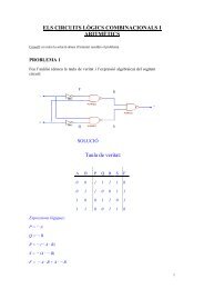
Pràctiques de Regulació Automàticay (t) = 10 + 5e −t cos (ωt + 0.5) on: 0 ≤ t ≤ 10Desenvolupeu un fitxer de script que dibuixi la resposta temporal de y ∼ t en una mateixagràfica pels valors de ω = 1,3,10 (rad/s), de dues maneres diferents, incloent en la gràficael següent:Títol: y (t) = 10 + 5 exp (−t) ∗ cos (ωt + 0.5)Etiqueta de l’eix t: Temps (s)Etiqueta de l’eix y: y (t) (rad/s)ReixetaText:ω = 1, ω = 3, ω = 10 (en un lloc aprop de la traça corresponent)1.5 Operació polinòmicaDonats els polinomis següents:P 1 (s) = s 3 + 2s 2 + 10 P 2 (s) = s + 11. Obteniu els polinomis A (s) i B (s) tals que:A (s) = P 1 (s) P 2 (s)B (s) = P 1 (s) + P 2 (s)2. Calculeu A (1) i B (0).3. Trobeu els valors de s que fan A (s) = 0.1.6 Modelització de sistemes dinàmics amb MatlabConsidereu el sistema de la Figura 1-1 amb:G (s) =1s 2 + 1.5s + 1G c1 (s) = 10G c2 (s) = 10 sCalculeu la funció de transferència Y (s)s + 1per a H (s) = 1 i per a H (s) =R (s) s + 2 , utilitzantles funcions series, paralell, cloop i feedback.1.7 Modelització de sistemes dinàmics amb SimulinkConsideru el sistema de la Figura 1-1 amb H (s) = 1. Desenvolupeu un programa ambSimulink per a una entrada r (t) de graó unitari i visualitzeu la resposta y (t) ∼ t per0 ≤ t ≤ 10 (temps de simulació).2Pràctica 1:Introducció al Matlab/Simulink. Modelat de sistemes dinàmics.

Pràctiques de Regulació AutomàticaFigura 1-11.8 Modelització d’un pèndul invertitFigura 1-2La dinàmica del pèndul invertit de la Figura 1-2 es descriu per les següents equacionsdiferencials no lineals:(M + m)ẍ + bẋ + ml¨θcosθ − ml ˙θ 2 sinθ = F(I + ml 2 )¨θ + mglsinθ = −mlẍcosθessent:Massa del carro:M = 0.5 KgMassa del pèndul:m = 0.2 KgFricció del carro:b = 0.1 N/m/sLongitud del centre de masses del pèndul: l = 0.3 mInèrcia del pèndul: I = 0.006 Kg · m 2Força aplicada al carro:FCoordenada de posició del carro: xAngle del pèndul respecte a la vertical: θSecció 1.8: Modelització d’un pèndul invertit 3

Pràctiques de Regulació Automàtica1. Construïu un esquema de Simulink que representi les equacions dinàmiques del sistemadel pèndul invertit essent la sortida del sistema l’angle θ i l’entrada del sistema la forçaF .2. Feu la linealització de les equacions dinàmiques, suposant que θ = π + φ, és a dir queφ representa un angle petit respecte a la posició vertical cap amunt i el punt de treballés θ ∗ = π o sigui φ = 0. Així es poden fer les següents aproximacions: cos θ ≃ −1,sin θ = −φ i ˙θ 2 ≃ 0. Obteniu la funció de transferència entre F i φ.4Pràctica 1:Introducció al Matlab/Simulink. Modelat de sistemes dinàmics.

2. ANÀLISI DE SISTEMES DE CONTROLAMB MATLAB/SIMULINK2.1 Objectius1. Familiaritzar-se amb el Matlab/Simulink.2. Utilitzar les eines que proporciona el Matlab/Simulink per analitzar els sistemes linealsen llaç obert i realimentats.2.2 Estudi previUn cop llegida la pràctica contesta les qüestions:• Tot i que existeix la funció step de Matlab per donar una entrada graó unitari a unsistema, com utilitzaries la funci lsim per fer el mateix.• Fes l’algorisme ( o diagrama de fluxe) dels 2 scripts demanats a la secció 2.3.22.3 Anàlisi de sistemes de control amb MatlabConsidereu un sistema de control amb una funció de transferència i una equació d’estat comla següent:{num (s)·x (t) = Ax (t) + Bu (t)G (s) = ⇐⇒den (s)y (t) = Cx (t) + Du (t)2.3.1 Resposta transitòria en el domini temporal• step5

Pràctiques de Regulació AutomàticaObtenir la resposta temporal del sistema a un graó unitari.• impulse>> step(num, den)>> step(A, B, C, D)>> [y, x, t] = step(num, den);>> [y, x, t] = step(A, B, C, D);>> plot(t, y)>> t = t i : δt : t f ;>> [y, x, t] = step(num, den, t);>> [y, x, t] = step(A, B, C, D, iu, t);>> plot(t, y)Obtenir la resposta temporal del sistema a un impuls.• lsim>> impulse(num, den)>> impulse(A, B, C, D)>> [y, x, t] = impulse(num, den);>> [y, x, t] = impulse(A, B, C, D);>> plot(t, y)>> t = t i : δt : t f ;>> [y, x, t] = impulse(num, den, t);>> [y, x, t] = impulse(A, B, C, D, iu, t);>> plot(t, y)Obtenir la resposta temporal del sistema a una entrada donada u(t).• stepfun>> t = t i : δt : t f ;>> u = u(t);>> [y, x] = lsim(num, den, u, t);>> [y, x] = lsim(A, B, C, D, u, t);>> plot(t, y)Crear un graó unitari que tingui una funció temporal tal com:{ 1 per t ≥ t0u(t) =0 per t < t 0>> t = t i : δt : t f ;>> u = stepfun(t, t 0 );Amb l’ús conjunt de stepfun i lsim, es pot obtenir la resposta temporal del sistemaa un graó unitari amb qualsevol temps d’inici.6 Pràctica 2: Anàlisi de sistemes de control amb Matlab/Simulink

Pràctiques de Regulació Automàtica• dcgainCalcular el guany k del sistema en el régim estable.>> k = dcgain(num, den)>> k = dcgain(A, B, C, D)2.3.2 Resposta transitòria en el domini freqüencial• bodeObtenir el diagrama de Bode.>> bode(num, den)>> bode(A, B, C, D)>> [mag, phase, w] = bode(num, den);>> [mag, phase, w] = bode(A, B, C, D);>> w = logspace(N min , N max , punts);>> bode(num, den, w)>> bode(A, B, C, D, iu, w);>> [mag, phase, w] = bode(num, den, w);>> [mag, phase, w] = bode(A, B, C, D, iu, w);>> w = freqint(num, den, punts);>> bode(num, den, w)>> [mag, phase, w] = bode(num, den, w);>> w = freqint(A, B, C, D, iu, punts);>> bode(A, B, C, D, iu, w);>> [mag, phase, w] = bode(A, B, C, D, iu, w);2.3.3 Pols i zeros• pzmapObtenir la localizació dels pols i zeros gràficament i els seus valors corresponents.>> pzmap(num, den)>> pzmap(A, B, C, D)>> [p, z] = pzmap(num, den);>> [p, z] = pzmap(A, B, C, D);Secció 2.3: Anàlisi de sistemes de control amb Matlab 7

Pràctiques de Regulació Automàticagraó unitari, rampa i parabola per 0 ≤ t ≤ 10. Representeu les respostes de y ∼ t perk = 0.1,1,10 i poseu títol, etiqueta i text a cada figura.2.4.4 Simplificació del sistemaConsidereu un sistema amb funció de transferència:G o (s) =1(s + 20) (s 2 + 0.5s + 1)1. Representeu gràficament la localització dels pols i zeros de G o (s) i determineu si existeixla dominació d’uns pols respecte als altres. Valoreu la possibilitat de reduir l’ordredel sistema i obteniu la funció de transferència d’ordre reduit G r (s). Representeu enuna figura les respostes temporals dels sistemes original G o (s) i reduit G r (s) a ungraó unitari i compareu els resultats.2. Representeu en una figura els diagrames de Bode dels sistemes original G o (s) i reduitG r (s) pel rang de freqüència [ 10 −2 , 10 2] i indiqueu en quin rang de freqüència ésvàlida la simplificació del sistema.2.4.5 Estabilitat i errors estacionarisConsidereu el sistema de control de la Figura 2-1 sense pertorbació (D (s) = 0) amb:C (s) = k sG (s) =1(s + 20) (s 2 + 0.5s + 1)1. Creeu un programa iteratiu de tipus script, amb el guany k del controlador com avariable, per comprovar l’estabilitat del sistema en llaç tancat mitjançant el criteride Rouht-Hurwitz i determieu el límit k lim a partir del qual el sistema realimentatresulta inestable.2. Amb tres guanys diferents k que generin respostes temporals estables, calculeu elserrors de posició, velocitat i acceleració, determineu el tipus del sistema i comenteula influència de k als errors estacionaris.2.4.6 Sistema de control pertorbatConsidereu el sistema de control de la Figura 2-1 amb:G (s) =1(s + 20) (s 2 + 0.5s + 1)Secció 2.4: Treballs a realitzar 9

Pràctiques de Regulació Automàtica1. Quan s’utilitza un controlador P amb C (s) = 10, obteniu amb Matlab la respostadel sistema y ∼ t a una consigna graó unitari amb temps d’inici t 0 = 1 s. i auna pertorbació graó unitari amb temps d’inici t 0 = 5 s. S’estabilitza la resposta delsistema a y = 1? Doneu explicacions sobre els resultats obtinguts utilitzant el teoremadel valor final.2. Repetiu els treballs anteriors y creeu un programa amb Simulink per comprobar elresultat que s’obté quan s’utilitza un controldor PI amb C (s) = 10 + 5 s .10 Pràctica 2: Anàlisi de sistemes de control amb Matlab/Simulink