Teoremas de Thevenin y Norton - Escuela Politécnica Superior

More documents

Recommendations

Info

Métodos y teoremas fundamentales de análisis tensiones de nudo (caso de estar entre dos nudos ajenos al de referencia, según indica la Fig. 3.12b). Por lo tanto, cada generador ideal asporta una nueva y sencilla ecuación o relación entre las tensiones objeto de análisis. Obsérvese, sin embargo, que para poder plantear la 1ª Ley de Kirchhoff en un nudo en el que confluya un generador de tensión, es necesario tener en cuenta la corriente que lo atraviesa, corriente que se convierte en una nueva incógnita del problema. Así, en el ejemplo mostrado en la Fig. 3.12a, la aplicación de la 1ª Ley de Kirchhoff a los dos nudos seleccionados resulta en las ecuaciones y sistema: Nudo A: Nudo B: VA VA −VB I1 − − = 0 Z Z I E 1 3 VB VA −VB − + = 0 Z Z 2 3 ⎡ 1 1 1 ⎤ + − ⎡ I ⎤ ⎢Z Z Z ⎥ ⎡VA ⎤ ⎢ I ⎥ E 1 1 1 ⎢ V ⎥ ⎣ ⎦ ⎢ ⎥⎣ B⎦ ⎢ − + ⎥ ⎣ Z3 Z2 Z3⎦ 1 1 3 3 ⇒ = ⎢ ⎥ , donde I E es la corriente (desconocida) que atraviesa el generador ideal de tensión; por lo tanto, el sistema de dos ecuaciones presenta tres incógnitas. Análogamente, en el ejemplo mostrado en la Fig. 3.12b, la aplicación de la 1ª Ley de Kirchhoff resulta en: Nudo A: Nudo B: VA I1 + IE − = 0 Z VB −I2 −IE − = 0 Z 1 2 ⎡ 1 ⎤ 0 ⎡ I + I ⎤ ⎢Z ⎥ ⎡V ⎤ 1 E 1 A ⇒ ⎢ I2 I ⎥ = ⎢ ⎥ E 1 ⎢ V ⎥ ⎣− − ⎦ ⎢ ⎥⎣ B⎦ ⎢ 0 ⎣ Z 2 ⎥ ⎦ La regla para considerar la presencia de un generador ideal de tensión resulta inmediata: en primer lugar se le asocia una corriente incógnita en el sentido de su polo positivo; a continuación esta corriente se incluye en la matriz de corrientes siguiendo la misma regla que para un generador de corriente. En definitiva, el método sistemático de análisis por tensiones permite de este modo plantear directamente las ecuaciones asociadas a los nudos del circuito. Estas ecuaciones, junto con la relación entre tensiones de nudo que permite plantear cada generador ideal de tensión, forman globalmente un sistema de ecuaciones que permite obtener tanto el valor de las tensiones de nudo como el de la corriente que atraviesa el generador ideal de tensión. 3.2.4 Dualidad Es inmediato observar que el desarrollo del método de los nudos es muy similar al del método de las mallas: prácticamente consiste en intercambiar los conceptos de corriente de malla por tensión de nudo, las magnitudes de generadores ideales de tensión por las de los generadores ideales de corriente, y las impedancias de las ramas que forman una malla por las admitancias de las ramas que confluyen en un nudo. Por lo demás, el procedimiento es idéntico, ya que las relaciones entre tensiones, corrientes e impedancias son las mismas que entre corrientes, tensiones y admitancias. En este sentido se suele decir que ambos métodos son duales. La elección de uno u otro método para resolver un circuito dado dependerá principalmente del número de ecuaciones que involucre cada uno. 13
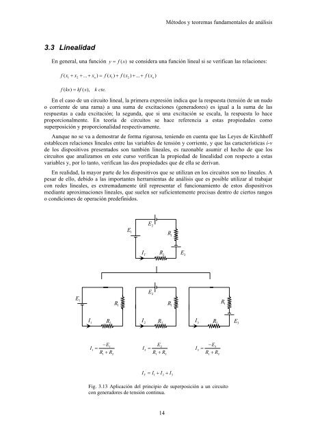
Métodos y teoremas fundamentales de análisis 3.3 Linealidad En general, una función y = f (x) se considera una función lineal si se verifican las relaciones: f( x + x + ... + x ) = f( x ) + f( x ) + ... + f( x ) 1 2 n 1 2 n f( kx) = kf( x), k cte . En el caso de un circuito lineal, la primera expresión indica que la respuesta (tensión de un nudo o corriente de una rama) a una suma de excitaciones (generadores) es igual a la suma de las respuestas a cada excitación; la segunda, que si una excitación se escala, la respuesta lo hace proporcionalmente. En teoría de circuitos se hace referencia a estas propiedades como superposición y proporcionalidad respectivamente. Aunque no se va a demostrar de forma rigurosa, teniendo en cuenta que las Leyes de Kirchhoff establecen relaciones lineales entre las variables de tensión y corriente, y que las características i-v de los dispositivos presentados son también lineales, es razonable asumir el hecho de que los circuitos que analizamos en este curso verifican la propiedad de linealidad con respecto a estas variables y, por lo tanto, verifican las dos propiedades que de ella se derivan. En realidad, la mayor parte de los dispositivos que se utilizan en los circuitos son no lineales. A pesar de ello, debido a las importantes herramientas de análisis que es posible utilizar al trabajar con redes lineales, es extremadamente útil representar el funcionamiento de estos dispositivos mediante aproximaciones lineales, que suelen ser suficientemente precisas dentro de ciertos rangos o condiciones de operación predefinidos. E 2 E 1 R 1 I T R 2 E 3 E 1 E 2 R1 R R 1 1 I1 R I 2 2 R I 2 3 R2 E 3 I 1 −E1 = R + R 1 2 I 2 E2 = R + R 1 2 I 3 −E3 = R + R 1 2 I = I + I + I T 1 2 3 Fig. 3.13 Aplicación del principio de superposición a un circuito con generadores de tensión continua. 14
Page 1: Universidad Autónoma de Madrid Esc
Page 4 and 5: Métodos y teoremas fundamentales d

Teoremas de Thevenin y Norton - Escuela Politécnica Superior

Create successful ePaper yourself

Delete template?

Save as template?