Cinemática inversa de un manipulador robótico con redes neuronales
Cinemática inversa de un manipulador robótico con redes neuronales
Cinemática inversa de un manipulador robótico con redes neuronales

You also want an ePaper? Increase the reach of your titles
YUMPU automatically turns print PDFs into web optimized ePapers that Google loves.
ENINVIE Encuentro <strong>de</strong> Investigación en IE, 4—5 Marzo, 2004 31<br />
ENINVIE – UAZ 2004<br />
Encuentro <strong>de</strong> Investigación en Ingeniería Eléctrica<br />
Zacatecas, Zac, Marzo 4 —5, 2004<br />
Cinemática <strong>inversa</strong> <strong>de</strong> <strong>un</strong> <strong>manipulador</strong> robótico<br />
<strong>con</strong> re<strong>de</strong>s <strong>neuronales</strong><br />
Víctor Martín Hernán<strong>de</strong>z Dávila<br />
Centro <strong>de</strong> estudios,<br />
Unidad Académica <strong>de</strong> Estudios Nucleares, UAZ, ZACATECAS ZAC-98000.<br />
TEL: +(492)9227043, ext. 16, correo-e: victorh@cantera.reduaz.mx<br />
Unidad Ingeniería Eléctrica, UAZ, ZACATECAS ZAC-98000.<br />
TEL: +(492)9239407, ext. 169, correo-e: victorh@cantera.reduaz.mx<br />
PhD. Jorge Samuel Benitez Read<br />
Centro <strong>de</strong> estudios,<br />
Instituto Nacional <strong>de</strong> Investigaciones Nucleares.<br />
TEL: +5553297200, ext. 2432 correo-e: jsbr@nuclear.inin.mx<br />
Resumen — Se muestra la resolución <strong>de</strong> la cinematica <strong>inversa</strong> <strong>de</strong> <strong>un</strong> <strong>manipulador</strong> robótico <strong>de</strong> 5 grados<br />
<strong>de</strong> libertad uasando re<strong>de</strong>s <strong>neuronales</strong>.<br />
Abstract —A neural processed inverse kinematics of robot manipulators with 5 DOF is shown here.<br />
Palabras clave — Re<strong>de</strong>s Neuronales(RN), retropropagación, cinemática, Manipulador Robótico(MR).<br />
I. INTRODUCCIÓN<br />
NVESTIGAR el comportamiento <strong>de</strong> mo<strong>de</strong>los <strong>de</strong> <strong>manipulador</strong>es robóticos es <strong>un</strong>a tarea interesante<br />
I que siempre tiene <strong>un</strong>a <strong>con</strong>stante en su mo<strong>de</strong>lado cinemático “La resolución <strong>de</strong> la cinemática<br />
<strong>inversa</strong> <strong>de</strong> <strong>un</strong> <strong>manipulador</strong> robótico se dificulta en f<strong>un</strong>ción <strong>de</strong>l incremento <strong>de</strong> los grados <strong>de</strong> libertad<br />
a tal grado que resulta imposible la solución analítica. Para la solución <strong>de</strong> la cinemática <strong>inversa</strong> se<br />
han usado aproximaciones numéricas [1] <strong>con</strong> bastante éxito; por otro lado, se han usado la lógica<br />
difusa y re<strong>de</strong>s <strong>neuronales</strong> para lograr dicha aproximación [4,5]. En este trabajo resolvemos la<br />
cinemática <strong>inversa</strong> <strong>de</strong> <strong>un</strong> <strong>manipulador</strong> robótico <strong>de</strong> 5 grados <strong>de</strong> libertad usando <strong>un</strong>a red neuronal <strong>de</strong><br />
topología 3 entradas 2 capas ocultas <strong>de</strong> 15 neuronas y <strong>un</strong>a capa <strong>de</strong> salida <strong>de</strong> 4 neuronas (15, 15, 4) y<br />
usando como base <strong>de</strong> <strong>con</strong>ocimiento el mo<strong>de</strong>lo analítico <strong>de</strong> la cinemática directa <strong>de</strong>l <strong>manipulador</strong>. El<br />
robot utilizado es el Scorbot ER-III <strong>de</strong>l <strong>de</strong>partamento <strong>de</strong> automatización <strong>de</strong>l Instituto Nacional <strong>de</strong><br />
Investigaciones nucleares ININ.<br />
II. PRINCIPIO TEÓRICO<br />
31
ENINVIE Encuentro <strong>de</strong> Investigación en IE, 4—5 Marzo, 2004 32<br />
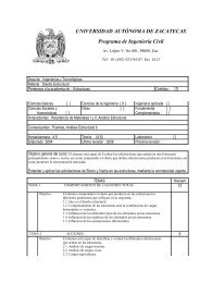
A partir <strong>de</strong> las características geométricas <strong>de</strong>l MR Scorbot ER-III se <strong>de</strong>sarrollará su mo<strong>de</strong>lo<br />
cinemático directo e inverso.<br />
A. Mo<strong>de</strong>lo cinemático directo<br />
Para obtener el mo<strong>de</strong>lo se utilizó la representación Denavit– Hartenberg [2,3,7]. La coor<strong>de</strong>nada<br />
<strong>de</strong> referencia se colocó en el eje <strong>de</strong> giro <strong>de</strong>l hombro, a <strong>un</strong>a distancia <strong>de</strong> 349 mm <strong>de</strong> la base física y<br />
se eliminó <strong>un</strong> grado <strong>de</strong> libertad (giro <strong>de</strong> la muñeca) ya que no <strong>con</strong>tribuye a la posición espacial <strong>de</strong>l<br />
MR. Por lo que ahora el mo<strong>de</strong>lo solo <strong>con</strong>tará <strong>con</strong> 4 grados <strong>de</strong> libertad.<br />
y 0<br />
z 0<br />
a 1<br />
x 0<br />
x 1<br />
x 2<br />
x 3<br />
a 3<br />
y 1<br />
a 2<br />
y 2<br />
y 3<br />
y 4<br />
θ 2<br />
θ 3<br />
θ 4<br />
a 4<br />
x 4<br />
Figura 1- Mo<strong>de</strong>lo cinemático <strong>de</strong> línea <strong>de</strong>l <strong>manipulador</strong> robótico.<br />
Las características físicas <strong>de</strong>l brazo son las siguientes<br />
Articulación<br />
( i )<br />
a α d θ<br />
1 a (16) π/2 0 θ 1 (310º)<br />
2 a (221) 0 0 θ 2 (170º)<br />
3 a (221) 0 0 θ 3 (300º)<br />
4 a (145) 0 0 θ 4 (180º)<br />
El mo<strong>de</strong>lo <strong>de</strong>l brazo es<br />
Tabla 1-Características <strong>de</strong>l <strong>manipulador</strong> robótico.<br />
Τ 0<br />
4<br />
[ ]<br />
[ ]<br />
⎡cc 1 234 − cs 1 234 s1 c1 ac 2 2+ ac 3 23+ ac 4 234 + ac 1 1⎤<br />
⎢<br />
⎥<br />
1 234 1 234 1 1 2 2 3 23 4 234 1 1<br />
0 1 2 3<br />
= = ⎢sc −ss − c s ac+ ac + ac + as<br />
A A A A<br />
⎥<br />
1 2 3 4<br />
⎢ s234 c234 0 a2s2+ a3s23+<br />
a4s234<br />
⎥<br />
⎢<br />
⎥<br />
⎣ 0 0 0 1<br />
⎦<br />
El siguiente arreglo nos da la orientación.<br />
(1)<br />
32
ENINVIE Encuentro <strong>de</strong> Investigación en IE, 4—5 Marzo, 2004 33<br />
n x = c 1 c 234 s x = -c 1 s 234 a x = s 1<br />
n y = s 1 c 234 s y = -s 1 s 234 a y = - c 1 (2)<br />
n z = s 234 s z = c 234 a z = 0<br />
Y el siguiente arreglo muestra la posición <strong>de</strong> la herramienta <strong>con</strong> respecto a las coor<strong>de</strong>nadas base:<br />
p x = c 1 [a 2 c 2 + a 3 c 23 + a 4 c 234 ] + a 1 c 1<br />
p y = s 1 [a 2 c 2 + a 3 c 23 + a 4 c 234 ] + a 1 s 1 (3)<br />
p z = a 2 s 2 + a 3 s 23 + a 4 s 234<br />
B. Mo<strong>de</strong>lo cinemático inverso<br />
A partir <strong>de</strong> las ecuaciones <strong>de</strong> posición <strong>de</strong>l mo<strong>de</strong>lo cinemático directo se <strong>de</strong>sarrolla el mo<strong>de</strong>lo<br />
cinemático inverso, haciendo uso <strong>de</strong> <strong>un</strong>a variable extra (φ) que es el ángulo <strong>de</strong> la herramienta <strong>con</strong><br />
respecto a la horizontal <strong>de</strong> la base <strong>de</strong>l robot.<br />
Y<br />
θ<br />
1=<br />
tan −1<br />
(4)<br />
X<br />
( a + a c ) PW −a<br />
s PW<br />
2 3 3 y 3 3 x<br />
( a + a c ) PW + a s PW<br />
2 3 3 x 3 3 y<br />
−1<br />
θ = tan<br />
(5)<br />
2<br />
2<br />
( ± 1−c<br />
3<br />
)<br />
2a<br />
a<br />
−1<br />
2 3<br />
θ<br />
3<br />
= tan<br />
(6)<br />
2<br />
2 2 2<br />
( PWx<br />
) + ( PW<br />
y<br />
) −a2<br />
−a3<br />
θ<br />
4<br />
φ − θ2<br />
− θ3<br />
= (7)<br />
III. DESCRIPCIÓN DE LA RED NEURONAL<br />
Una vez que se tiene el mo<strong>de</strong>lo cinemático directo se hace <strong>un</strong> programa en Matlab que genere las<br />
tablas <strong>de</strong> <strong>con</strong>ocimiento y que lleve a cabo el proceso <strong>de</strong> entrenamiento <strong>de</strong> la red neuronal.<br />
Las características <strong>de</strong> la red neuronal son las siguientes:<br />
- Multicapa <strong>con</strong> fase <strong>de</strong> entrenamiento fuera <strong>de</strong> línea y utiliza el algoritmo <strong>de</strong> retropropagación<br />
<strong>de</strong> error para la fase <strong>de</strong> entrenamiento [8].<br />
- 3 valores <strong>de</strong> entrada X, Y y Z.<br />
- 2 capas ocultas <strong>de</strong> 15 neuronas y <strong>un</strong>a <strong>de</strong> salida <strong>de</strong> 4 neuronas Θ 1 , Θ 2 , Θ 3 y Θ 4 .<br />
- Para el entrenamiento se usa el algoritmo <strong>de</strong> gradiente <strong>de</strong>scen<strong>de</strong>nte <strong>con</strong> momento igual a 0.65<br />
y razón variable <strong>de</strong> aprendizaje entre 0.001 y 0.01 [9,10].<br />
- La red neuronal se entrenará en Matlab usando la utileria <strong>de</strong> re<strong>de</strong>s <strong>neuronales</strong> y el algoritmo<br />
trainbpx.<br />
Ya entrenada la red neuronal para <strong>un</strong>a <strong>de</strong>terminada trayectoria, se le presentan los datos X, Y y Z<br />
a la red neuronal <strong>de</strong> cada <strong>un</strong>o <strong>de</strong> los p<strong>un</strong>tos en don<strong>de</strong> la herramienta <strong>de</strong>l robot <strong>de</strong>be pasar. La<br />
siguiente curva es <strong>un</strong> cálculo hecho <strong>con</strong> el mo<strong>de</strong>lo cinemático directo y probado <strong>con</strong> la red neuronal<br />
sin usar el mo<strong>de</strong>lo teórico <strong>de</strong> la cinemática <strong>inversa</strong>. Se comprueba este análisis por medio <strong>de</strong> la<br />
prueba <strong>de</strong> la Chi-cuadrada [6].<br />
33
ENINVIE Encuentro <strong>de</strong> Investigación en IE, 4—5 Marzo, 2004 34<br />
Haciendo uso <strong>de</strong>l mo<strong>de</strong>lo teórico <strong>de</strong> cinemática directa, se obtienen 10 datos en don<strong>de</strong> se muestran<br />
los valores cartesianos así como sus respectivos ángulos <strong>de</strong> las articulaciones <strong>de</strong>l MR<br />
Valores <strong>de</strong> entrada Cálculo cinemático teórico Respuesta <strong>de</strong> la RN<br />
X Y Z θ 1 θ 2 θ 3 θ 4 θ 1 θ 2 θ 3 θ 4<br />
603.0000 0.0000 0 0 0 0 0 0.0324 0.1863 0.3241 0.0085<br />
467.7941 82.4847 0 10 0 0 0 10.2678 -0.165 0.2455 0.0313<br />
446.3639 162.4632 0 20 0 0 0 19.6288 0.2526 -0.295 -0.031<br />
411.3712 237.5053 0 30 0 0 0 29.8397 0.0846 -0.180 -0.025<br />
363.8792 305.3309 0 40 0 0 0 40.1658 -0.132 0.0910 0.0021<br />
305.3309 363.8792 0 50 0 0 0 50.2318 -0.141 0.2029 0.0199<br />
237.5053 411.3712 0 60 0 0 0 60.0394 0.0029 0.0964 0.0183<br />
162.4632 446.3639 0 70 0 0 0 69.8402 0.1038 -0.097 -0.002<br />
82.4847 467.7941 0 80 0 0 0 79.8914 0.055 -0.170 -0.021<br />
0.0000 603.0000 0 90 0 0 0 90.0990 -0.060 0.1050 0.0075<br />
Tabla 2.-Valores cinemáticos teóricos y respuesta <strong>de</strong> la red neuronal<br />
Figura 2- Gráfica <strong>de</strong>l mo<strong>de</strong>lo cinemático y la respuesta <strong>de</strong> la RN para <strong>un</strong> arco.<br />
Usando la prueba <strong>de</strong> Chi cuadrada<br />
H 0 :<br />
Los datos <strong>de</strong> la RN se distribuyen <strong>de</strong> la misma forma que los datos <strong>de</strong>l mo<strong>de</strong>lo<br />
cinemático.<br />
Ha : Los datos <strong>de</strong> la RN no se distribuyen <strong>de</strong> la misma forma que los datos <strong>de</strong>l mo<strong>de</strong>lo<br />
cinemático.<br />
34
ENINVIE Encuentro <strong>de</strong> Investigación en IE, 4—5 Marzo, 2004 35<br />
Nivel <strong>de</strong> <strong>con</strong>fianza utilizado: 0.95<br />
Grados <strong>de</strong> libertad n-1: 9<br />
Valor <strong>de</strong> tablas: 2.733<br />
Calculando los valores <strong>de</strong> Chi cuadrada para cada ángulo se obtiene:<br />
Valor <strong>de</strong> Chi cuadrada para θ 1 : 0.0522<br />
Valor <strong>de</strong> Chi cuadrada para θ 2 : 0.0219<br />
Valor <strong>de</strong> Chi cuadrada para θ 3 : 0.0411<br />
Valor <strong>de</strong> Chi cuadrada para θ 4 : 0.0005<br />
Como el valor <strong>de</strong> Chi cuadrada para cada ángulo es inferior al <strong>de</strong> tablas se acepta H 0 .<br />
IV. CONCLUSIONES Y TRABAJO FUTURO<br />
Concluyendo, los datos <strong>de</strong> salida <strong>de</strong> la RN <strong>de</strong>scriben correctamente los planteados por el mo<strong>de</strong>lo<br />
cinemático.<br />
Se pue<strong>de</strong> afirmar, que solo basta resolver el mo<strong>de</strong>lo cinemático directo <strong>de</strong>l MR y aplicar <strong>un</strong>a RN<br />
que resuelva el mo<strong>de</strong>lo teórico <strong>de</strong> cinemática <strong>inversa</strong>, sin necesidad <strong>de</strong> resolver el mo<strong>de</strong>lo analítico.<br />
RECONOCIMIENTOS<br />
Al Instituto Nacional <strong>de</strong> Investigaciones Nucleares por permitirnos la entrada y facilitarnos el<br />
<strong>manipulador</strong> robótico Scorbot ER-III.<br />
REFERENCIAS<br />
[1] P. J. Alsina, N. S. Gehlot “Direct and inverse kinematics of robotic manipulator based on modular neural networks ”, ICARCV 94,<br />
p. 1743-7, Vol. 3<br />
[2] Manseur, R., Dot Keith “ A fast algorithm for reverse kinematics analysis of robot manipulator “ International Journal of Robotics<br />
Research, 7:3, 1998.<br />
[3] Bazerghi A., Gol<strong>de</strong>nberg A. “ An exact kinematics mo<strong>de</strong>l of PUMA 600 manipulator “ IEEE transaction on Systems, Man an<br />
Cybernetics, Vol. 14, No. 3 1984.<br />
[4] Zhuang, H., Roth Z. “ A complete and parametrically <strong>con</strong>tinuous kinematics mo<strong>de</strong>l for robot manipulators “ , Vol. 8, No. 4, 1992<br />
[5] S. Dreiseitl, T. Kobik “ Neural processed inverse kinematics of robot manipulators ”, ICARCV 94, pp. 1748-51, Vol. 3.<br />
[6] Gorinevsky D., Connoly T. “ Comparations of some neural network and scattered data aproximations : The inverse manipulator<br />
kinematics example “ Neural computation Vol. 6, Num. 3, pp. 521-542.<br />
[7] Xiao-Xuyu “ Efficient backpropagation learning rate and momentum “ Neural Networks, Vol. 10, No. 3 pp. 517-527, 1997.<br />
[8] Lee L. “ Trainning feedforward neural networks : An algorithm givin improved generalitation “ Neural Networks, Vol. 10, No. 1,<br />
pp. 61-68, 1997.<br />
[9] Magoulas D., G; Vrahatis N., M.; Androulakis S., G. “ Effective backpropagation training with variable stepsize “Neural Networks,<br />
Vol. 10, No. 1, pp. 69-82, 1997.<br />
[10] Schittenkopf C.; Deco G.; Bra<strong>un</strong>er W. “ Two strategies to avoid overfitting in feedforward networks “Neural Networks, Vol. 10,<br />
No. 3, pp. 505-516, 1997.<br />
35