Capítulo 1 Métodos de residuos ponderados Funciones de prueba ...

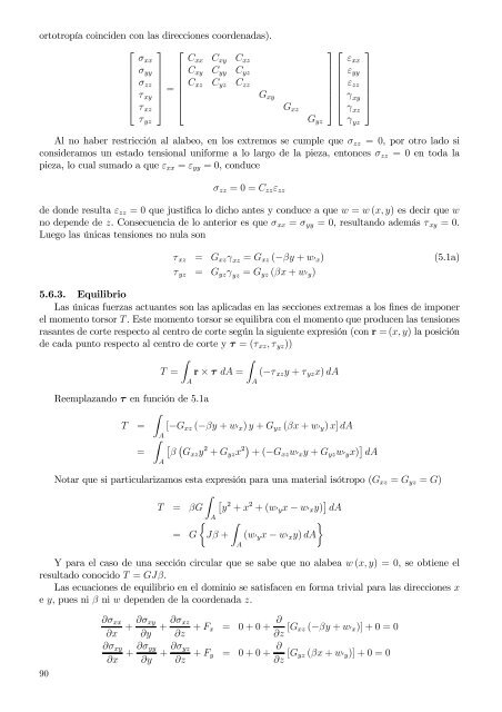
ortotropía coinciden con las direcciones coordenadas).
⎡ ⎤ ⎡
⎤ ⎡
σ xx C xx C xy C xz
σ yy
C xy C yy C yz
σ zz
⎢ τ xy
=
C xz C yz C zz ⎥ ⎢
G xy ⎥ ⎢
⎣ τ xz
⎦ ⎣
G xz
⎦ ⎣
τ yz
G yz
Al no haber restricción al alabeo, en los extremos se cumple que σ zz = 0, por otro lado si
consideramos un estado tensional uniforme a lo largo de la pieza, entonces σ zz = 0 en toda la
pieza, lo cual sumado a que ε xx = ε yy = 0, conduce
σ zz = 0 = C zz ε zz
de donde resulta ε zz = 0 que justifica lo dicho antes y conduce a que w = w (x, y) es decir que w
no depende de z. Consecuencia de lo anterior es que σ xx = σ yy = 0, resultando además τ xy = 0.
Luego las únicas tensiones no nula son
ε xx
ε yy
ε zz
γ xy
γ xz
γ yz
τ xz = G xz γ xz = G xz (−βy + w′ x) (5.1a)
τ yz = G yz γ yz = G yz (βx + w′ y)
5.6.3. Equilibrio
Las únicas fuerzas actuantes son las aplicadas en las secciones extremas a los fines de imponer
el momento torsor T . Este momento torsor se equilibra con el momento que producen las tensiones
rasantes de corte respecto al centro de corte según la siguiente expresión (con r = (x, y) la posición
de cada punto respecto al centro de corte y τ = (τ xz , τ yz ))
∫
∫
T = r × τ dA = (−τ xz y + τ yz x) dA
A
Reemplazando τ en función de 5.1a
∫
T = [−G xz (−βy + w′ x) y + G yz (βx + w′ y) x] dA
∫A
[ (
= β Gxz y 2 + G yz x 2) + (−G xz w′ xy + G yz w′ yx) ] dA
A
Notar que si particularizamos esta expresión para una material isótropo (G xz = G yz = G)
∫
[
T = βG y 2 + x 2 + (w′ yx − w′ xy) ] dA
A
{ ∫
}
= G Jβ + (w′ yx − w′ xy) dA
A
Y para el caso de una sección circular que se sabe que no alabea w (x, y) = 0, se obtiene el
resultado conocido T = GJβ.
Las ecuaciones de equilibrio en el dominio se satisfacen en forma trivial para las direcciones x
e y, pues ni β ni w dependen de la coordenada z.
A
⎤
⎥
⎦
90
∂σ xx
+ ∂σ xy
∂y
∂x
∂σ xy
∂x + ∂σ yy
∂y
+ ∂σ xz
∂z + F x = 0 + 0 + ∂ ∂z [G xz (−βy + w′ x)] + 0 = 0
+ ∂σ yz
∂z + F y = 0 + 0 + ∂ ∂z [G yz (βx + w′ y)] + 0 = 0