Capítulo 1 Métodos de residuos ponderados Funciones de prueba ...
Capítulo 1 Métodos de residuos ponderados Funciones de prueba ...
Capítulo 1 Métodos de residuos ponderados Funciones de prueba ...

You also want an ePaper? Increase the reach of your titles
YUMPU automatically turns print PDFs into web optimized ePapers that Google loves.
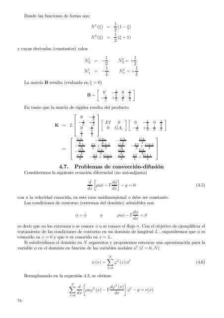
Don<strong>de</strong> las funciones <strong>de</strong> forma son:<br />
N 1 (ξ) = 1 (1 − ξ)<br />
2<br />
N 2 (ξ) = 1 (ξ + 1)<br />
2<br />
y cuyas <strong>de</strong>rivadas (constantes) valen<br />
N 1<br />
′ ξ = − 1 2<br />
N 1<br />
′ x = − 1 L<br />
N 2<br />
′ ξ = +1 2<br />
N 2<br />
′ x = + 1 L<br />
La matriz B resulta (evaluada en ξ = 0)<br />
[ 0 −<br />
1<br />
B =<br />
− 1 + 1 L 2<br />
1<br />
0<br />
L L<br />
1 1<br />
L 2<br />
]<br />
En tanto que la matriz <strong>de</strong> rigi<strong>de</strong>z resulta <strong>de</strong>l producto<br />
⎡ ⎤<br />
0 − 1 L [ ] [ K = L ⎢ − 1 + 1 L 2 ⎥ EI 0 0 −<br />
1<br />
⎣ 1<br />
0 ⎦ 0 GA<br />
L<br />
c − 1 + 1 L 2<br />
=<br />
⎡<br />
⎢<br />
⎣<br />
1<br />
L<br />
GA c<br />
L<br />
− GAc<br />
2<br />
− GAc<br />
L<br />
1<br />
2<br />
GA c<br />
− EI<br />
2 L<br />
1<br />
0<br />
L L<br />
1 1<br />
L 2<br />
− GA 0c<br />
− GA c GA c<br />
2 L<br />
2<br />
EI<br />
+ GAcL GA c<br />
− EI + GAcL<br />
L 2 2 L 2<br />
GA c GA c GA c<br />
+<br />
2<br />
GA L<br />
2<br />
cL GA c EI<br />
2 2 L<br />
+ GA cL<br />
2<br />
4.7. Problemas <strong>de</strong> convección-difusión<br />
Consi<strong>de</strong>remos la siguiente ecuación diferencial (no autoadjunta)<br />
[<br />
d<br />
ρuφ − Γ dφ ]<br />
− q = 0 (4.5)<br />
dx dx<br />
con u la velocidad conocida, en este caso unidimensional u <strong>de</strong>be ser constante.<br />
Las condiciones <strong>de</strong> contorno (extremos <strong>de</strong>l dominio) admisibles son:<br />
φ = ¯φ o ρuφ − Γ dφ<br />
dx = ¯σ<br />
es <strong>de</strong>cir que en los extremos o se conoce φ o se conoce el flujo σ. Con el objetivo <strong>de</strong> ejemplificar el<br />
tratamiento <strong>de</strong> las condiciones <strong>de</strong> contorno en un dominio <strong>de</strong> longitud L , supondremos que φ es<br />
conocido en x = 0 y que σ es conocido en x = L.<br />
Si subdividimos el dominio en N segmentos y proponemos entonces una aproximación para la<br />
variable φ en el dominio en función <strong>de</strong> las variables nodales φ I (I = 0..N)<br />
⎤<br />
⎥<br />
⎦<br />
]<br />
φ (x) =<br />
N∑<br />
ϕ I (x) φ I (4.6)<br />
I=0<br />
78<br />
Reemplazando en la expresión 4.5, se obtiene<br />
N∑<br />
I=0<br />
[<br />
]<br />
d<br />
ρuϕ I (x) − Γ dϕI (x)<br />
φ I − q = r(x)<br />
dx<br />
dx