Capítulo 1 Métodos de residuos ponderados Funciones de prueba ...

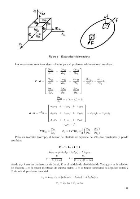
Figura 6
Elasticidad tridimensional
Las ecuaciones anteriores desarrolladas para el problema tridimensional resultan:
⎡
∂σ 11
+ ∂σ 12
+ ∂σ ⎤
13
∂x 1 ∂x 2 ∂x 3
∂σ 21
∇ · σ =
+ ∂σ 22
+ ∂σ 23
= ∂σ ij
t i = ∂σ ji
t i
∂x 1 ∂x 2 ∂x 3
∂x j ∂x j
⎢
⎣ ∂σ 31
+ ∂σ 32
+ ∂σ ⎥
⎦
33
∂x 3 ∂x 2 ∂x 3
⎡
σ · n = σ T n =
⎢
⎣
∂σ ij
∂x j
+ ρ (b i − a i ) = 0
⎤
σ 11 ν 1 + σ 12 ν 2 + σ 13 ν 3
σ 21 ν 1 + σ 22 ν 2 + σ 23 ν 3
⎥
⎦ = σ ijν j t i = σ ij ν i t j
σ 31 ν 1 + σ 32 ν 2 + σ 33 ν 3
σ ij ν j = f i
(∇u) ij
= ∂u i
∂x j
ε ij = (∇ s u) ij
= 1 2
( ∂uj
+ ∂u )
i
∂x i ∂x j
Para un material isótropo, el tensor de elasticidad depende de sólo dos constantes y puede
escribirse
D =2µ I+λ 1 ⊗ 1
D ijkl = µ (δ ik δ jl + δ il δ jk ) + λ δ ij δ kl
E
Eν
µ =
λ =
2 (1 + ν) (1 + ν) (1 − 2ν)
donde µ y λ son los parámetros de Lamé, E es el módulo de elasticidad de Young y ν es la relación
de Poisson. I es el tensor identidad de cuarto orden, 1 es el tensor identidad de segundo orden y
⊗ denota el producto tensorial
σ ij = D ijkl ε kl = [µ (δ ik δ jl + δ il δ jk ) + λ δ ij δ kl ] ε kl
σ ij = 2µ ε ij + δ ij λ ε kk
97