tarea 1 - Facultad de IngenierÃa
tarea 1 - Facultad de IngenierÃa
tarea 1 - Facultad de IngenierÃa

Create successful ePaper yourself
Turn your PDF publications into a flip-book with our unique Google optimized e-Paper software.
A P U N T E S D E Á L G E B R A L I N E A L<br />
Universidad Nacional Autónoma <strong>de</strong> México<br />
<strong>Facultad</strong> <strong>de</strong> Ingeniería.<br />
M.I. Luis Cesar Vázquez Segovia<br />
Grupo:<br />
Semestre: 2010-2
TEMA 1.- ESPACIOS VECTORIALES.<br />
Definición.<br />
Sea V un conjunto no vacío y sea (k, +, *) un campo. Se dice que V es un espacio vectorial<br />
sobre k si están <strong>de</strong>finidas dos leyes <strong>de</strong> composición, llamadas adición y multiplicación por<br />
un escalar, tales que:<br />
I) La adición asigna a cada pareja or<strong>de</strong>nada (ū, ) <strong>de</strong> elementos <strong>de</strong> V un único<br />
elemento ū + V, llamado la suma <strong>de</strong> ū y .<br />
II) ū, , V: ū+( + ) = (ū+ )+ .<br />
III) ō V tal que ō + = , V.<br />
IV) V – V tal que – + = ō<br />
V) ū, α: u+ = + ū<br />
VI)<br />
La multiplicación por un escalar asigna a cada pareja or<strong>de</strong>nada (α,v) <strong>de</strong><br />
elementos <strong>de</strong> α k y V un único elemento α k llado el producto <strong>de</strong> α por<br />
.<br />
VII) α k; ū, V: α(ū+ ) = αū+ α<br />
VIII) α,β k; V: (α+β) = α + β<br />
IX) α,β k; V: α(β ) = (αβ)<br />
X) Si 1 es la unidad <strong>de</strong> k 1 = , V<br />
A los elementos <strong>de</strong> V se llama vectores y a los <strong>de</strong> k se les llama escalares.<br />
Ejemplo.<br />
R 3 ; F,f: R→R P n M 2x2<br />
√ √ √ √ I<br />
√ √ √ √ II<br />
√ √ √ √ III<br />
√ √ √ √ IV<br />
√ √ √ √ V<br />
√ √ √ √ VI<br />
√ √ √ √ VII<br />
√ √ √ √ VIII<br />
√ √ √ √ IX<br />
√ √ √ √ X<br />
Ejemplo.<br />
Sea el conjunto S = {ax 2 + ax + b )│a,b R} en R y las leyes <strong>de</strong> adición y multiplicación por<br />
un escalar usuales. Determinar si S es un espacio vectorial.
i) CERRADURA<br />
P 1 = a 1 x 2 + a 1 x + b 1 ; P 2 = a 2 x 2 + a 2 x + b 2<br />
P 1 + P 2 = (a 1 +a 2 )x 2 + (a 1 +a 2 )x + (b 1 +b 2 ) se cumple S R<br />
ii) ASOCIATIVIDAD<br />
P 1 + (P 2 + P 3 ) = (P 1 + P 2 ) + P 3<br />
P 1 + [(a 2 + a 3 )x 2 + (a 2 + a 3 )x + (b 2 + b 3 )] = [(a 1 + a 2 )x 2 + (a 1 + a 2 )x + (b 1 + b 2 )] + P 3<br />
(a 1 +a 2 +a 3 )x 2 + (a 1 +a 2 +a 3 )x + (b 1 +b 2 + b 3 ) = (a 1 +a 2 +a 3 )x 2 + (a 1 +a 2 +a 3 )x + (b 1 +b 2 + b 3 )<br />
Se cumple<br />
iii) E ELEMENTO IDENTICO<br />
ō + P 1 = P 1<br />
(ex 2 + e 1 x + ei 1 ) + (ax 2 + ax + b) = ax 2 + ax + b<br />
(e + a)x 2 + (e + a)x + (ei + b) = ax 2 + ax + b<br />
e + a = a e = 0<br />
e + a = a e = 0 (0)x = (0)x 2 +(0)x +0<br />
ei + b = b ei = 0<br />
iv) E ELEMENTO INVERSO<br />
- + = 0 + p = 0<br />
(Ix 2 + Ix + d) + (ax 2 + ax + b) = (0)x 2 +(0)x +0<br />
(I + a)x 2 + (I + a)x + (d + b) = (0)x 2 +(0)x +0<br />
I + a = 0 I = -a<br />
I + a = 0 I = -a - = = ax 2 + ax + b<br />
d+ b = 0 d = -b<br />
v) CONMUTATIVIDAD<br />
P 1 + P 2 = P 2 + P 1<br />
(a 1 +a 2 )x 2 + (a 1 +a 2 )x + (b 1 +b 2 ) = (a 2 +a 1 )x 2 + (a 2 +a 1 )x + (b 2 +b 1 )<br />
vi) MULTIPLICACIÓN POR UN ESCALAR<br />
αp = S<br />
αp = αax 2 + αax + αb S Se cumple<br />
vii) SUMA DE VECTORES POR UN ESCALAR<br />
α(P 1 + P 2 ) = αP 1 + αP 2
α*(a 1 +a 2 )x 2 + (a 1 +a 2 )x + (b 1 +b 2 )+ = (αa 1 x 2 + αa 1 x + αb 1 ) + (αa 2 x 2 + αa 2 x + αb 2 )<br />
(αa 1 + αa 2 )x 2 + (αa 1 + αa 2 )x + (αb 1 + αb 2 ) = (αa 1 + αa 2 )x 2 + (αa 1 + αa 2 )x + (αb 1 + αb 2 )<br />
Se cumple<br />
viii) SUMA DE ESCALARES POR UN VECTOR<br />
(α + β)p = αp + βp<br />
(α + β)a 1 x 2 + (α + β)a 1 x + (α + β)b 1 = (αa 1 x 2 + αa 1 x + αb 1 ) + (βa 1 x 2 + βa 1 x + βb 1 )<br />
(αa 1 + βa 1 )x 2 + (αa 1 + βa 1 )x + (αb 1 + βb 1 ) = (αa 1 + βa 1 )x 2 + (αa 1 + βa 1 )x + (αb 1 + βb 1 )<br />
Se cumple.<br />
ix) α(βp) = (αβ)p<br />
α (βax 2 + βax + βb) = αβax 2 + αβax + αβb<br />
αβax 2 + αβax + αβb = αβax 2 + αβax + αβb<br />
Se cumple<br />
X) UNIDAD DEL CAMPO<br />
1p = p<br />
1ax 2 + 1ax + 1b = ax 2 + ax + b<br />
Se cumple<br />
S es un campo vectorial<br />
-DEFINICIÓN DE SUBESPACIO.<br />
Sea V un espacio vectorial en K y sea S un subconjunto <strong>de</strong> V.<br />
S es un subespacio <strong>de</strong> V si es un espacio vectorial en K respecto a la adición y<br />
multiplicación por un escalar <strong>de</strong>finidas en V.<br />
Teorema<br />
Sea V un espacio vectorial en K y sea S un subconjunto <strong>de</strong> V.<br />
S es un subespacio <strong>de</strong> V si y solo si .<br />
1) ū + = S; Para todo ū, S<br />
2) αū = S; Para todo α K, ū S<br />
Demostración<br />
V = E 3<br />
S = Plano XY S = {(x, y, 0)│x, y R}<br />
Determine si S es un subespacio.<br />
Solución:<br />
1) ū + = S; Para todo ū, S<br />
(x 1 , y 1 , 0) + (x 2 , y 2 , 0) = (x 1 + x 2 , y 1 + y 2 ,0) S Se cumple
2) αū = S; Para todo α K, ū S<br />
α(x 1 , y 1 , 0) = (αx 1 , αy 1 , 0) S Se cumple<br />
S es un subespacio vectorial <strong>de</strong> V<br />
Ejemplo<br />
Sea п = ,(x, y, z)│ x + y -z = 2; x, y, z R}<br />
Determinar si п es un espacio vectorial en R con las operaciones <strong>de</strong> adición <strong>de</strong> vectores y<br />
multiplicación por un escalar usuales.<br />
Solución:<br />
x + y -z = 2 ; z = x + y –2<br />
п = , (x, y, x + y -2)│x, y R}<br />
I) 1 = (x 1 , y 1 , x 1 + y 1 -2) ; 2 = (x 2 ,y 2 , x 2 + y 2 -2)<br />
1 + 2 = [x 1 + x 2, y 1 + y 2, (x 1 + x 2 ) + (y 1 + y 2 ) –4]<br />
п no es un espacio vectorial.<br />
Ejemplo.<br />
Sea el conjunto D = { │a, b R} <strong>de</strong>termine si D es un espacio vectorial con las<br />
leyes <strong>de</strong> composición <strong>de</strong> adición <strong>de</strong> vectores y multiplicación por un escalar usuales.<br />
Solución:<br />
i) 1 =<br />
a<br />
1<br />
0<br />
0<br />
b<br />
1<br />
2 =<br />
a<br />
2<br />
0<br />
0<br />
b<br />
2<br />
1 + 2 =<br />
a<br />
1<br />
0<br />
a<br />
2<br />
b<br />
1<br />
0<br />
b<br />
2<br />
D<br />
Se cumple<br />
ii) α 1 D<br />
α D Se cumple
Espacios R n<br />
D es un subespacio vectorial.<br />
R 2 = [(a, b)│a, b R]<br />
R 3 = [(a, b, c)│ a, b, c R]<br />
R 4 = [(a 1 , a 2 , a 3 , a 4 )│ a 1 , a 2 , a 3 , a 4 R]<br />
R n = [(a 1 , a 2 , a 3 , ..., a n )│ a 1 , a 2 , a 3 , ..., a n R]<br />
R´= [a│a R]<br />
COMBINACIÓN LINEAL.<br />
α 1+ β 2 =<br />
Definición.<br />
Un vector w es una combinación lineal <strong>de</strong> los vectores 1+ 2 + 3 ,..., n si pue<strong>de</strong> ser<br />
expresado en la forma = α 1 1 + α 2 2 ,..., +α n n don<strong>de</strong> α 1 ,α 2,..., α n son escalares.<br />
Ejemplo<br />
Sea = (3, 4, -2)<br />
[(1,2,0), (2,2,-2)]<br />
= α 1 + β 2<br />
= 1(1,2,0) + 1(2,2,1)<br />
[(1,1,-1), (1,2,0)]<br />
(3,4,-2) = α (1,1,-1) + β(1,2,0)<br />
(3,4,-2) = (α,α,-α) + (β,2β,0)<br />
(3,4,-2) = (α + β, α + 2β,-α)<br />
α + β =3<br />
α + 2β = 4 α = 2; β=1<br />
-α = -2<br />
Ejemplo.<br />
Sea = (6,7,5)<br />
Forma trinómica → = 6i + 7j +5k<br />
= 6(1, 0, 0) + 7(0, 1, 0) + 5(0, 0, 1)<br />
Ejemplo
Sea D = { │a, b R}<br />
{ , } a + b =<br />
Ejemplo<br />
R 2 = [(a, b)│a, b R]<br />
{(1,0), (1,1), (0,1)}<br />
α(1,0), β(1,1), γ(0,1) = (a, b)<br />
(α,0), (β, β), (0, γ) = (a, b)<br />
(α + β, β + γ) = (a, b)<br />
α + β = a<br />
β + γ = b<br />
Del 2° renglón<br />
β + γ = b ; γ = b - β<br />
Del 1° renglón<br />
α + β = a ; α = a – β β = β<br />
Solución<br />
α = a - k<br />
β = k<br />
γ = b – k<br />
k R<br />
Definición.<br />
Sea S = { 1, 2,...,<br />
n } un conjunto <strong>de</strong> vectores<br />
1) S es linealmente <strong>de</strong>pendiente si existen escalares α 1 ,α 2,..., α n , no todos son iguales a<br />
cero, tales que α 1 1 + α 2 2 +... + α n n = ō<br />
2) S es linealmente in<strong>de</strong>pendiente si la igualdad α 1 1 + α 2 2 +... + α n n = ō, solo se<br />
satisface con α 1 = α 2 =,..., = α n = 0<br />
Ecuación <strong>de</strong> <strong>de</strong>pen<strong>de</strong>ncia lineal<br />
α 1 1 + α 2 2 +... + α n n = ō<br />
B = {<br />
1<br />
0<br />
0<br />
0<br />
,<br />
0<br />
0<br />
0<br />
1<br />
}<br />
Para B
1 0<br />
α 1<br />
0 0<br />
0 0 0 0<br />
+ α 2<br />
0 1 0 0<br />
0<br />
1<br />
0<br />
0<br />
+<br />
0<br />
0<br />
0<br />
2<br />
=<br />
0 0<br />
0 0<br />
α 1 = 0; α 2 = 0<br />
1<br />
0<br />
0 =<br />
0 0<br />
2<br />
0 0<br />
B es linealmente in<strong>de</strong>pendiente<br />
Bп 2 = {(1, 0, 1), (0, 1, 1)}<br />
Teorema<br />
Sea S = { 1 , 2,..., n } un conjunto no vacío <strong>de</strong> vectores <strong>de</strong> un espacio vectorial V.<br />
El conjunto <strong>de</strong> todas las combinaciones lineales <strong>de</strong> vectores <strong>de</strong> S, <strong>de</strong>notado con L(S), es un<br />
subespacio <strong>de</strong> S.<br />
S = {(1, 2)} a(1, 2) = (a, 2a)<br />
F = L(S) F = {(a, 2a) │a R }<br />
Teorema<br />
Todo conjunto que contiene al vector ō es linealmente <strong>de</strong>pendiente.<br />
Demostración<br />
De la ecuación <strong>de</strong> <strong>de</strong>pen<strong>de</strong>ncia lineal α 1 1 , α 2 2 ,..., α i i ,..., α n n = ō ; α i = R<br />
El conjunto es linealmente <strong>de</strong>pendiente.<br />
Definición.<br />
Sea V un espacio vectorial en R, y sea G = { 1, 2,..., n } un conjunto <strong>de</strong> vectores <strong>de</strong> V. Se<br />
dice que G es un generador <strong>de</strong> V si para todo R existen escalares α 1 ,α 2 ,..., α n , tales que,<br />
= α 1 1 + α 2 2 +... + α n n .<br />
Definición.<br />
Se llama base <strong>de</strong> un espacio vectorial V a un conjunto generador <strong>de</strong> V que es linealmente<br />
in<strong>de</strong>pendiente.<br />
Teorema<br />
Sea V un espacio vectorial en K. Si B = { 1, 2,...,<br />
otra base <strong>de</strong> dicho está formada por n vectores.<br />
n } es una base <strong>de</strong> V, entonces cualquier
Definición<br />
Sea V un espacio vectorial en K. Si B = { 1, 2,...,<br />
dimensión n, lo cual <strong>de</strong>notamos con dimV = n<br />
n } es una base <strong>de</strong> V se dice que V es <strong>de</strong><br />
En particular, si V = { }; dimV = 0.<br />
Ejemplo<br />
R 2 = [(a, b)│a, b R]<br />
B = {(0, 1), (1, 0)} = (-3, 2)<br />
α(0, 1) + β(1, 0) = (-3, 2)<br />
(0, α) + (β, 0) = (-3, 2)<br />
(β, α) = (-3, 2) → por igualdad <strong>de</strong> vectores β = -3 y α = 2<br />
Vector <strong>de</strong> coor<strong>de</strong>nadas ( ) B = (α, β) = (2, -3)<br />
Definición<br />
Sea B = { 1, 2,..., n } una base <strong>de</strong> un espacio vectorial V en K, y sea V.<br />
Si = α 1 1 + α 2 2 +... + α n n , los escalares α 1 ,α 2 ,..., α n se llaman coor<strong>de</strong>nadas <strong>de</strong> en la<br />
base B, y el vector Kn ( ) B = ( α 1 ,α 2 ,..., α n ) T se llama vector <strong>de</strong> coor<strong>de</strong>nadas <strong>de</strong> en la<br />
base B.<br />
ESPACIOS ASOCIADOS A UNA MATRIZ.<br />
A =<br />
Espacio renglón asociado a A<br />
G = {(1, 0),(4, 2),(-1, 7)}<br />
L(G) = {a(1, 0), b(4, 2), c(-1, 7)│a, b, c R}<br />
4R1<br />
R2<br />
R1<br />
R3<br />
R2(1/<br />
2)<br />
7R2<br />
R3<br />
B = {(1,0), (0,1) }<br />
L(B) = {a(1,0) + b(0,1) } dim A R = 2<br />
A R =L(B) = {(a, b)│a, b R }<br />
Espacio columna
A = A T =<br />
B 1 = G 1 = {(1, 4, -1), (0, 2, 7)}<br />
Ac =L(G 1 ) = {a(1, 4, -1) + b(0, 2, 7)│a, b R }<br />
Corolario<br />
→ elemento genérico a(1, 4, -1) + b(0, 2, 7) = (a, 4a + 2b, -a + 7b)<br />
Ac = {(a, 4a + 2b, -a + 7b)│a, b R }<br />
Dim Ac = 1<br />
dim A R = dim A c<br />
Ejemplo<br />
R 2 = [(a, b)│a, b R]<br />
B 1 = {(1, 0), (0, 1)}; B 2 = {(0, 2), (2, 0)}<br />
Obtener los valores <strong>de</strong> coor<strong>de</strong>nadas <strong>de</strong>l vector = (-2, 3)<br />
G ={ , , }<br />
Para G<br />
β 1 + β 2 + β 3 =<br />
1<br />
0<br />
0 0 + 2<br />
0<br />
0<br />
2<br />
+<br />
0 0<br />
0<br />
3<br />
=<br />
0 0<br />
0 0<br />
1 2<br />
0<br />
0<br />
2 3<br />
=<br />
0 0<br />
0 0<br />
1 2 = 0 1 2<br />
2 3 = 0 3 2 2 = k; 1 3 k<br />
G es linealmente <strong>de</strong>pendiente.<br />
B y G son conjuntos generadores<br />
V; B genera V; linealmente in<strong>de</strong>pendiente → Base
V; G genera V; linealmente <strong>de</strong>pendiente → Generador<br />
Algoritmo <strong>de</strong> obtención <strong>de</strong> bases<br />
P 2 = {ax 2 + bx + c)│a, b, c R}<br />
B = {x 2 , x, 1}<br />
R 2 = [(a, b)│a, b R]<br />
B = {(1, 0), (0, 1)}<br />
M 2x1 = { │a, b R} B = { 1 0 , 0<br />
1 }<br />
Sea el espacio п = {(x, y, z)│x + y -z = 2; x, y, z R}<br />
x + y -z = 0 п 2 = {(x, y, x + y)│ x, y, z R}<br />
z = x + y<br />
Matriz <strong>de</strong> transición<br />
B<br />
M 1 B 2<br />
1= α 1 1 + α 2 2<br />
2= β 1 1 + β 2 2<br />
(1,0) = α 1 (0,2)+ α 2 (2,0)<br />
(1,0) = (2α 2 , 2α 1 α 2 (2,0)<br />
2α 2 = 1 → α 2 = ½ 2α 1 = 0 → α 1 = 0<br />
1 = (1,0) = 0(0,2) + ½(2,0)<br />
( 1 ) B2 = (0, ½) T<br />
2 = (0,1) = β 1 (0,2) + β 2 (2,0) (0,1) = (2β 2 , 2β 1 )<br />
2 β 2 = 0 → β 2 = 0 2β 1 = 0 → β 1 = ½<br />
2 = (0,1) = ½(0,2) + 0(2,0)<br />
( 2 ) B2 = (½, 0) T<br />
1 = 0 1 + ½ 2<br />
2 = ½ 1 + 0 2
M A B = ( ) A = ( ) B<br />
( ) A = (M A B ) -1 ( ) B<br />
(M A B ) = (M A B ) -1 ( ) A = M B A ( ) B<br />
3. A =<br />
A T =<br />
B AC = {(1, 0, 0), (0 ,1 ,0), (0, 0, 1)}<br />
a(1, 0, 0) + b(0, 1, 0) + c(0, 0, 1) = (a, b, c) → elemento genérico<br />
A C = {(a, b, c)│a, b, c R}<br />
Solución: los 3 R<br />
Teorema<br />
Los espacios que tienen la misma dimensión se llaman isomorfos.<br />
R 3 = [(a, b, c)│a, b, c R]; dim R 3 = 3; B R 3 = {(1, 0, 0), (0, 1, 0), (0, 0, 1)}<br />
P 2 = {ax 2 + ax + b)│a, b R} dim R 2 = 2; B R<br />
2<br />
= {(x 2 + x + 1)<br />
F 1 (ax 2 + bx + c) = (a, b, c)<br />
1.-<br />
M = { │a, b, c R}; dim M =3; B M ={ , , }<br />
F 2 = (a, b, c)<br />
2.-<br />
V = { │a, b R}<br />
Solución:<br />
B V ={ , } dim V = 2<br />
A no es base; B no es base; C si es base<br />
3.-
f = (0, 1, -1, 3)<br />
f = (1, 0, 1, 0) Es linealmente in<strong>de</strong>pendiente<br />
ESPACIOS DE FUNCIONES F<br />
Sea el conjunto H = {e x , e -x , e 2x }<br />
L(H) = {ae x + be -x + ce 2x a, b, c R}<br />
Determine si H es linealmente in<strong>de</strong>pendiente<br />
Wronskiano<br />
W =<br />
e<br />
e<br />
e<br />
x<br />
x<br />
x<br />
e<br />
e<br />
e<br />
x<br />
x<br />
x<br />
e<br />
2x<br />
2x<br />
2 e =<br />
4e<br />
2x<br />
x<br />
e (-1) 2<br />
e<br />
e<br />
x<br />
x<br />
2e<br />
4e<br />
2x<br />
2x<br />
+<br />
x<br />
e (-1) 3<br />
e<br />
e<br />
x<br />
x<br />
2e<br />
4e<br />
2x<br />
2x<br />
+<br />
x<br />
e 2 (-<br />
1) 4 x<br />
e e<br />
x x<br />
e e<br />
x<br />
W = e x (-4e x -2e x ) –e -x (4e 3x -2e 3x ) + e 2x (e 0 + e 0 )<br />
W = -6e 2x –2e 2x +2e 2x<br />
W = -6e 2x W ≠ 0<br />
H es linealmente in<strong>de</strong>pendiente<br />
Sea el conjunto <strong>de</strong> funciones reales <strong>de</strong> variable real {f 1 , f 2 , ..., f n }<br />
De la ecuación <strong>de</strong> <strong>de</strong>pen<strong>de</strong>ncia lineal α 1 f 1 + α 2 f 2 +... + α n f n = 0<br />
Para x = x 1 α 1 f(x 1 ) + α 2 f(x 1 ) +... + α n f(x 1 ) = 0<br />
Para x = x 2 β 1 f(x 2 ) + β 2 f(x 2 ) +... + β n f(x 2 ) = 0<br />
Para x = x n λ 1 f(x n ) + λ 2 f(x n ) +... + λ n f(x n ) = 0<br />
Teorema<br />
Sea {f 1 , f 2 , ..., f n } un conjunto <strong>de</strong> n funciones <strong>de</strong> variable real, <strong>de</strong>rivables al menos n-1<br />
veces en el intervalo (a, b); y sea
W=<br />
f<br />
f<br />
f<br />
1<br />
´<br />
1<br />
(n-1)<br />
1<br />
(x)<br />
(x)<br />
<br />
(x)<br />
f<br />
f<br />
f<br />
2<br />
´<br />
2<br />
(n-1)<br />
2<br />
(x)<br />
(x)<br />
<br />
(x)<br />
<br />
<br />
<br />
<br />
f<br />
f<br />
f<br />
n<br />
´<br />
n<br />
(n-1)<br />
n<br />
(x)<br />
(x)<br />
<br />
(x)<br />
Si W(x 0 ) ≠ 0 para algún x 0 (a, b), entonces el conjunto <strong>de</strong> funciones es linealmente<br />
in<strong>de</strong>pendiente <strong>de</strong> dicho intervalo.<br />
Si W(x) = 0 no <strong>de</strong>ci<strong>de</strong>.<br />
Ejemplo<br />
Investigar la <strong>de</strong>pen<strong>de</strong>ncia lineal <strong>de</strong>l siguiente conjunto.<br />
F = {2sen 2 x, -cos 2 x, 3}<br />
W(x) =<br />
2<br />
2sen<br />
x<br />
4senxcos<br />
x<br />
2<br />
4sen<br />
x<br />
4cos<br />
2<br />
x<br />
2cos xsenx<br />
2cos<br />
2<br />
cos<br />
x<br />
2<br />
x<br />
sen<br />
2<br />
x<br />
3<br />
0<br />
0<br />
=<br />
4senxcosx<br />
4sen<br />
2<br />
x<br />
4cos<br />
2<br />
x<br />
2cosxsenx<br />
2cos<br />
2<br />
x<br />
sen<br />
2<br />
x<br />
W(x) = 3[4senxcosx (2cos 2 x -2sen 2 x) – (-4sen 2 x + 4cos 2 x)( 2cosxsenx)]<br />
W(x) = 3(0) = 0 → no <strong>de</strong>ci<strong>de</strong>.<br />
F = {2sen 2 x, sen 2 x -1, 3}<br />
α(2sen 2 x) + β(sen 2 x –1) + γ(3) = (0) 2sen 2 x + 0<br />
(2α+ β)sen 2 x + (3γ –β) = (0) 2sen 2 x + 0<br />
(2α+ β) = 0 → α = -β/2<br />
(3γ –β) = 0 → γ = β/3 β = k<br />
α = -k/2<br />
β = k<br />
γ = k/3<br />
Es linealmente <strong>de</strong>pendiente.<br />
Nota: 1 regla <strong>de</strong> correspon<strong>de</strong>ncia y W = 0 es linealmente <strong>de</strong>pendiente.<br />
Ejemplo<br />
Sea el conjunto <strong>de</strong> funciones, <strong>de</strong>termine si es linealmente <strong>de</strong>pendiente o in<strong>de</strong>pendiente<br />
en el intervalo indicado.<br />
D = {h, f, g}
f(x) =<br />
x 2 ; si x 0; ū≠<br />
Ejemplo<br />
Sea R 2 = [(a, b)│a, b R] y<br />
a) f(ū│ ) = [(a 1 , b 1 )│(a 2 , b 2 )] = a 1 a 2 + b 1 b 2<br />
b) h(ū│ ) = [(a 1 , b 1 )│(a 2 , b 2 )] = 2a 1 a 2 + b 1 b 2<br />
Determine si f, h son productos internos.<br />
3) (αū│ ) = α(ū│ )<br />
*(αa 1 , αb 1 )│(a 2 , b 2 )+ = α(2a 1 a 2 + b 1 b 2 )<br />
2αa 1 a 2 + αb 1 b 2 se cumple<br />
4) (ū│ ) > 0<br />
[(a 1 , b 1 )│(a 1 , b 1 )] = 2a 1 2 + b 1<br />
2<br />
> 0<br />
se cumple<br />
h es producto interno
Propieda<strong>de</strong>s <strong>de</strong>l producto interno.<br />
Sea V un espacio vectorial en C y sea ( │ ) un producto interno en V, entonces ū, V y<br />
α C.<br />
1) (ū│α ) = (ū│ )<br />
2) (ū│ū) = R +<br />
3) ( │ū) = 0 = (ū│ )<br />
4) (ū│ū) = 0 ↔ ū =<br />
NORMA DE UN VECTOR<br />
= ( │ ) 1/2 ; La norma es un número real.<br />
Propieda<strong>de</strong>s <strong>de</strong> una norma.<br />
Sí V es un espacio vectorial con producto interno, entonces ū, V y α C.<br />
1. > 0<br />
2. = 0 ↔ =<br />
3. = ; = =<br />
4. +<br />
Ejemplo<br />
Sea un generador <strong>de</strong> R 3 ,el conjunto G = {(2, 0, 0), (0, 0, 4), (0, 1, 0), (1, 2, 3)}. Determine un<br />
conjunto ortogonal a partir <strong>de</strong> G utilizando el producto escalar ordinario.<br />
Gran Shmidt.<br />
1 = 1 = (2, 0, 0)<br />
2 = 2 -<br />
v<br />
w<br />
2<br />
1<br />
w<br />
w<br />
1<br />
1<br />
2 = (0, 0, 4) -<br />
(0,0,4) (2,0,0)<br />
(2,0,0) (2,0,0)<br />
= (0, 0, 4) - ( 4<br />
0 )(2, 0, 0) = (0, 0, 4)<br />
3 = 3 -<br />
v<br />
w<br />
3<br />
1<br />
w<br />
w<br />
1<br />
1<br />
1 -<br />
v<br />
w<br />
3<br />
2<br />
w<br />
w<br />
2<br />
2<br />
2<br />
3 = (0, 1, 0) -<br />
(0,1,0) (2,0,0)<br />
4<br />
(2, 0, 0) -<br />
(0,1,0) (0,0,4)<br />
(0,0,4) (0,0,4)<br />
(0, 0, 4)
3 = (0, 1, 0) - (0, 0, 0) - ( 16<br />
0 )(0, 0, 4) = (0, 1, 0)<br />
4 = 4 -<br />
v<br />
w<br />
4<br />
1<br />
w<br />
w<br />
1<br />
1<br />
1 -<br />
v<br />
w<br />
4<br />
2<br />
w<br />
w<br />
2<br />
2<br />
2 -<br />
v<br />
w<br />
4<br />
3<br />
w<br />
w<br />
3<br />
3<br />
3<br />
4 = (1, 2, 3)<br />
(1,2,3) (2,0,0)<br />
4<br />
(2, 0, 0) -<br />
(1,2,3) (0,0,4)<br />
16<br />
(0, 0, 4) -<br />
(1,2,3) (0,1,0)<br />
(0,1,0) (0,1,0)<br />
(0, 1, 0)<br />
4 = (1, 2, 3) - (1, 0, 0) - (0, 0, 3) - (0, 2, 0) = (0, 0, 0)<br />
G 0 = {(2, 0, 0), (0, 0, 4), (0, 1, 0), (0, 0, 0)}<br />
B ORT = {(2, 0, 0), (0, 0, 4), (0, 1, 0)}<br />
B ORTN = {(1, 0, 0), (0, 0, 1), (0, 1, 0)}<br />
Ejemplo<br />
En el espacio vectorial <strong>de</strong> matrices simétricas <strong>de</strong> or<strong>de</strong>n 2 se <strong>de</strong>fine el siguiente producto<br />
a1 b1 a<br />
2<br />
b2<br />
interno<br />
= a 1 a 2 + 2b 1 b 2 + c 1 c 2 y el conjunto G = { , ,<br />
b c b c<br />
1 1 2 2<br />
, . Determine un conjunto ortogonal a partir <strong>de</strong> G<br />
B ORT = { , , , .<br />
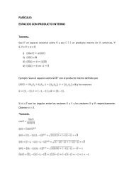
Ejemplo.<br />
Para el espacio vectorial C 2 se <strong>de</strong>fine el producto interno (ū│ ) =<br />
= (y 1 , y 2 ) C 2 don<strong>de</strong> i es el conjugado <strong>de</strong> yi.<br />
2<br />
i 1<br />
xi yi = (x 1 , x 2 )<br />
a) Determinar las normas <strong>de</strong> los vectores = (4+2i, 5 – 6i), = (3-2i, -2i), = (-2-2i, i)<br />
=<br />
1/2<br />
= = = = 9
=<br />
= =<br />
=<br />
= = 3<br />
b) Obtener el ángulo entre y<br />
1/2<br />
1/2<br />
= angcos<br />
R( 4 10 i)<br />
3 17<br />
= angcos<br />
4<br />
3 17<br />
= 108.86°<br />
Propieda<strong>de</strong>s <strong>de</strong> la distancia entre dos vectores.<br />
Si V es un espacio vectorial con producto interno, entonces ū, V.<br />
1. d(ū, ) 0<br />
2. d(ū, ) = 0 y solo si ū =<br />
3. d(ū, ) = d( , ū)<br />
4. d(ū, ) d(ū, ) + d( , )<br />
=<br />
1/2<br />
=<br />
1/2<br />
=<br />
1/2<br />
= = 8<br />
Teorema <strong>de</strong> Pitágoras.<br />
Sea V un espacio con producto interno y sean ū, V. Si ū y son ortogonales, entonces:<br />
2 =<br />
2 +<br />
2<br />
Teorema<br />
Desigualdad <strong>de</strong> Cauchy-Schwarz<br />
Sea V un espacio vectorial en C y sea ( │ ) un producto interno en V, entonces ū, V:<br />
2 ≤ don<strong>de</strong> es el módulo <strong>de</strong> . A<strong>de</strong>más, la igualdad se<br />
cumple si y solo si son linealmente in<strong>de</strong>pendientes.<br />
Ejemplo<br />
1.- Sea B = { 1 , 2} una base <strong>de</strong> un espacio vectorial.
Determine a partir <strong>de</strong> V una base ortogonal.<br />
B ORT = { 1, 2} 1 = 1<br />
Proy vect =<br />
v v<br />
2 1<br />
v v<br />
1 1<br />
1<br />
2 = 2 - Proy vect<br />
2 = 2 -<br />
v<br />
w<br />
2<br />
1<br />
w<br />
w<br />
1<br />
1<br />
1 B ORT =<br />
w<br />
w<br />
w<br />
1 2<br />
,<br />
w<br />
1 2<br />
w =<br />
Bw = {(1, 1, 0), (0, 2, 1)}<br />
Ortogonalizado<br />
1 = 1 = (1, 1, 0)<br />
2 = 2 -<br />
v<br />
w<br />
2<br />
1<br />
w<br />
w<br />
1<br />
1<br />
= 1 = (0, 2, 1) -<br />
(0,2,1) (1,1,0)<br />
(1,1,0) (1,1,0)<br />
(1, 1, 0)<br />
= (0, 2, 1) - ( 2<br />
2 )(1, 1, 0) = (-1, 1,1)<br />
Bw ORT = {(1, 1, 0), (-1, 1, 1)}<br />
Bw ORT = { }<br />
w = = q ei ei<br />
+ q e2 e2<br />
1 1<br />
1 1<br />
= ( 0,2, 6) (1,1,0) (1,10)<br />
+ ( 0,2, 6) ( 1,1,1) ( 1,1,1 )<br />
2 2<br />
3 3<br />
1<br />
2 6 1<br />
= (0 + ) (1,10)<br />
+ ( 0 ) ( 1,1,1 )<br />
2<br />
3 3 3
4<br />
= (1, 1,0) - ( 1,1,1 )<br />
3<br />
7 1 4<br />
= ( , , )<br />
3 3 3<br />
2.- Para el producto interno usual en R 3 , obtener el cumplimiento ortogonal S 1 <strong>de</strong> cada uno<br />
<strong>de</strong> los subespacios siguientes <strong>de</strong> R 3 y dar una interpretación geométrica <strong>de</strong> dichos<br />
complementos.<br />
a) S 1 = {(0,0,z)│z R}<br />
= (a, b, c) R 3 {(0, 0, z)│(a, b, c)} = 0<br />
zc = 0<br />
c = 0<br />
a = k<br />
b = t<br />
S ´<br />
1 = {(k, t, 0)│k, t R}<br />
b) S 2 = {(x, x,0)│x R}<br />
= (a, b, c) R 3 {(x, x, 0)│(a, b, c)} = 0<br />
ax + bx = 0<br />
x(a +b) = 0<br />
a = -b ; a = -t<br />
c = k<br />
b = t<br />
S ´2 = {(-t, t, k)│t, k R}
3.- Sea w = │a, b R} un subespacio <strong>de</strong> las matrices cuadradas <strong>de</strong> or<strong>de</strong>n dos en<br />
R con producto interno <strong>de</strong>finido por (A│ B) = tr(AB T ).<br />
Obtener la matriz perteneciente a W más próximo a M =<br />
Bw = { , }<br />
1 = 1 =<br />
0<br />
1<br />
1<br />
0<br />
2 = 2 =<br />
v<br />
w<br />
2<br />
1<br />
w<br />
w<br />
1<br />
1<br />
w 1 = -<br />
1<br />
1<br />
0<br />
0<br />
0<br />
1<br />
2<br />
0<br />
1<br />
0<br />
0<br />
2<br />
0<br />
2<br />
0<br />
2<br />
│ = tr = tr<br />
1<br />
0<br />
0<br />
2<br />
= 0<br />
│ = = 5<br />
2 = - 5<br />
0<br />
=<br />
= { , }<br />
Bw ORT = { , }<br />
21α + 11β + 5γ = 0<br />
α = - 11<br />
21 k - 5 t; β = k; γ = t<br />
21<br />
w = {(- 11<br />
21 k - 5 21 t )x2 +kx + t | k, t R }<br />
b) = - ´<br />
4.- Dado el producto interno en R 2 <strong>de</strong>finido por = u 1 v 1 - u 1 v 2 - u 2 v 1 + 3u 2 v 2 don<strong>de</strong><br />
= (u 1 , u 2 , u 3 ) y = (v 1 , v 2 ).
a) Obtener el valor <strong>de</strong> K R tal que<br />
la distancia entre los vectores = (1, 3) y = (k, 4) sea igual a .<br />
b) Con el vector <strong>de</strong> k obtenido,<br />
verificar que los vectores y <strong>de</strong>l inciso anterior cumplan la <strong>de</strong>sigualdad <strong>de</strong> Cauchy-<br />
Schwarz.<br />
a) d(ū, ) =<br />
= (k-1, 1)<br />
1/2 =<br />
1/2<br />
=<br />
2<br />
k 2k 1 k+1-k 1 3 1/2 =<br />
2<br />
k 4k 6 1/2<br />
2 =<br />
2<br />
k 4k 6 ;<br />
2<br />
k 4k 4 = 0; ( k-2)( k-2) = 0; k = 2<br />
b)<br />
2 ≤<br />
= 28 (28) 2 ≤ (22)(36)<br />
= 22 784 ≤ 792<br />
= 36 Es linealmente in<strong>de</strong>pendiente.<br />
5.- Obtener una base ortogonal <strong>de</strong>l espacio vectorial F <strong>de</strong> los polinomios <strong>de</strong> grado menor<br />
o igual a dos con coeficientes reales a partir <strong>de</strong> la base B = {1, 2t, 2 - 12t + 12t 2 }<br />
consi<strong>de</strong>rando el producto interno = p, q F<br />
1 = 1<br />
2 = 2t -<br />
2t 1<br />
11<br />
(1) = 2t -<br />
(2t |1) = = t 2 1 = 1 0<br />
(1 |1) = = t 1 = 1 0<br />
1<br />
1<br />
(1) = 2t – 1<br />
3 = 2 - 12t + 12t 2 -<br />
2<br />
2 12t 12t 1<br />
11<br />
(1) -<br />
2<br />
2 12t 12t 2t 1<br />
2t 1 2t 1<br />
(2t – 1)<br />
3 = 2 - 12t + 12t 2 -0 -0 = 2 - 12t + 12t 2<br />
(2 - 12t + 12t 2 |1) =<br />
1<br />
2<br />
(2 12t 12t )dt = 2t - 6t 2 + 4t 3 1 = 2- 6 + 4 = 0<br />
0<br />
0
(2t -1|2t -1) =<br />
(2 - 12t + 12t 2 |2t -1) =<br />
=<br />
1<br />
2<br />
(4t 4t 1)dt = 4 3 t3 - 2t 2 + t 1 = 4 0<br />
3 - 2 + 1 = 1 3<br />
0<br />
4 3 2<br />
6t 12t 8t 2t 1 0<br />
= 6 -12 + 8 -2 = 0<br />
1<br />
1<br />
2 3 2<br />
(4t 2 24t 12t+24t 12t )dt =<br />
0<br />
0<br />
3 2<br />
(24t 36t 16t 2)dt<br />
6.- Sea el sistema <strong>de</strong> ecuaciones lineales homogéneo y sea W el espacio solución <strong>de</strong> dicho<br />
sistema para el producto interno usual en R 3 , <strong>de</strong>terminar el complemento ortogonal w ,<br />
<strong>de</strong> W y escribir el vector (9, 1, 4) como la suma <strong>de</strong> un vector <strong>de</strong> W mas otro <strong>de</strong> w .<br />
-x + 3y -2z = 0<br />
x= 3y – 2z x = 3k -2t<br />
y = y y = k z = z; z = t<br />
W = {(3k -2t, k, t) │k, t b R}<br />
Bw ORT =<br />
1<br />
0<br />
5<br />
0<br />
2<br />
5<br />
,<br />
0<br />
1<br />
2<br />
1<br />
0<br />
2<br />
=<br />
2<br />
i 1<br />
M ei ei<br />
= M ei ei<br />
+ M e2 e2<br />
=<br />
2<br />
1<br />
1<br />
2<br />
1<br />
5<br />
1<br />
0<br />
0<br />
2<br />
1<br />
5<br />
1<br />
0<br />
0<br />
2<br />
+<br />
2<br />
1<br />
1<br />
2<br />
1<br />
2<br />
0<br />
1<br />
1<br />
0<br />
1<br />
2<br />
0<br />
1<br />
1<br />
0<br />
=<br />
1<br />
5<br />
1<br />
5<br />
tr<br />
2<br />
1<br />
1<br />
2<br />
1<br />
0<br />
0<br />
2<br />
1<br />
0<br />
0<br />
2<br />
+<br />
1<br />
5<br />
1<br />
5<br />
tr<br />
2<br />
1<br />
1<br />
2<br />
0<br />
1<br />
1<br />
0<br />
0<br />
1<br />
1<br />
0<br />
1 2<br />
= tr 5 4<br />
1<br />
0<br />
0<br />
2<br />
+<br />
1 1 tr<br />
2 1<br />
0<br />
1<br />
1<br />
0
=<br />
2<br />
5<br />
1<br />
1<br />
4<br />
5<br />
+<br />
0<br />
1<br />
0<br />
1<br />
=<br />
2<br />
5<br />
1<br />
1<br />
4<br />
5<br />
(p│ ) =<br />
2<br />
i 0<br />
p ( i)<br />
q(<br />
i)<br />
p(x), q(x) P 2<br />
W = {ax 2 + bx + c)│a, b, c R}<br />
a) Obtener w<br />
W = {ax 2 + ax + -a)│a R} P 2 = {αx 2 + βx + γ)│α, β, γ R}<br />
x<br />
2<br />
x<br />
ax<br />
2<br />
ax -a<br />
= 0<br />
= γ(-a) + (α + β + γ)(a) + (4α + 2β + γ)(5a)<br />
= -γa + αa + βa + γa + 20αa + 10βa + 5γa<br />
= a(4α + 2β + γ) = 0<br />
R 3 = [(a, b, c)│ a, b, c R]<br />
[(3k -2t, k, t) │(a, b, c)] = 0<br />
3ak -2at + kbt + c = 0<br />
k(3a +b) + t(-2a + c) = 0<br />
3a +b = 0 ↔ b = -3a<br />
-2a + c = 0 ↔ c = 2a<br />
w = {a, -3a, 2a)│a R}<br />
TRANSFORMACIONES LINEALES<br />
T: R 3 →R 2<br />
T(x, y, z) = (x, y)<br />
Definición<br />
Si V y W son espacios vectoriales, una función T: V→W recibe el nombre <strong>de</strong><br />
transformación, los espacios V y W se llaman, respectivamente dominio y codominio <strong>de</strong> la<br />
transformación.<br />
Ejemplo<br />
T(x, y, z) = (x, y) T: R 3 →R 2<br />
S(ax 2 + bx + c) =<br />
S: P 2 →D
Definición.<br />
Sea T: V→W una transformación<br />
1) Se llama recorrido <strong>de</strong> T al<br />
conjunto<br />
T(v) = { T( )│ V }<br />
2) Se llama núcleo <strong>de</strong> T al conjunto<br />
N(T) = { │T( ) = w}<br />
Ejemplo<br />
T: R 3 →R 2 <strong>de</strong>finida por T(x, y, z) = (x, y)<br />
Dominio: R 3<br />
Recorrido: R 2<br />
Núcleo: w<br />
T(x, y, z) = (0, 0) x = 0; y =0<br />
(x, y) = (0, 0)<br />
T(0, 0, z) = (0, 0) N(T) = {(0, 0, z)│z R }<br />
Definición.<br />
Sean V y W dos espacios vectoriales en K, una transformación T: V→W es lineal si 1, 2<br />
V y α K<br />
Superposición 1) T( 1 + 2) = T( 1 ) + T( 2 )<br />
Homogeneidad 2) T( 1) = αT( 1 )<br />
Ejemplo<br />
Para las siguientes transformaciones <strong>de</strong>terminar si son lineales o no.<br />
1.- T: R 3 →R 2 <strong>de</strong>finida por T(x, y, z) = (x, y)<br />
Solución:<br />
1) T( 1 + 2) = T( 1 ) + T( 2 )<br />
T( 1 + x 2 , y 1 + y 2 , z 1 + z 2 ) = ( 1 , y 1 ) + (x 2 , y 2 )<br />
( 1 + x 2 , y 1 + y 2 ) = ( 1 + x 2 , y 1 + y 2 ) Cumple<br />
2) T( 1) = αT( 1 )
T(αx, αy, αz) = α( 1 , y 1 )<br />
(αx, αy) = (α 1 , αy 1 )<br />
Cumple<br />
T es una transformación lineal.<br />
2.- S: P 2 →D; S(ax 2 + bx + c) =<br />
Solución:<br />
a<br />
0<br />
0<br />
c<br />
1) S( 1 + 2) = S( 1 ) + S( 2 )<br />
1 = a 1 x 2 + b 1 x + c 1 ; 2 = a 2 x 2 + b 2 x + c 2<br />
S [(a 1 + a 2 )x 2 a1<br />
+ (b 1 + b 2 )x + (c 1 + c 2 )] =<br />
0<br />
0<br />
c<br />
1<br />
+<br />
a<br />
2<br />
0<br />
0<br />
c<br />
2<br />
a<br />
1<br />
0<br />
a<br />
2<br />
c<br />
1<br />
0<br />
c<br />
2<br />
=<br />
a<br />
1<br />
0<br />
a<br />
2<br />
c<br />
1<br />
0<br />
c<br />
2<br />
Cumple<br />
2) S( 1) = αS( 1 )<br />
S(αa 1 x 2 a1<br />
0<br />
+ αb 1 x + αc 1 ) =α<br />
0 c<br />
a<br />
0<br />
1<br />
0<br />
c<br />
1<br />
=<br />
a<br />
0<br />
S es una transformación lineal.<br />
3.- F: R 2 →R 2<br />
1<br />
0<br />
c<br />
1<br />
1<br />
Cumple<br />
F(x, y) = (x 2 , y) 1 = ( 1 , y 1 ) 2 = (x 2 , y 2 )<br />
1) F( 1 + 2) = F( 1 ) + F( 2 )<br />
F( 1 + x 2 , y 1 + y 2 ) = ( x , y 1 ) + ( x , y 2 )<br />
[( 1 + x 2 ) 2 2<br />
, y 1 + y 2 ] = [ x<br />
1 + x 2 2 , y 1 + y 2 ]<br />
F no es una transformación lineal<br />
2<br />
1<br />
2<br />
2<br />
Teorema.
Si T: V→W es una transformación lineal entonces T( v) = w<br />
Teorema.<br />
Si T: V→W es una transformación lineal entonces<br />
1) T(v) es un subespacio <strong>de</strong> W<br />
2) N(T) es un subespacio <strong>de</strong> T<br />
Ejemplo<br />
T: R 3 →M <strong>de</strong>finida por T(a, b, c) =<br />
a<br />
b<br />
1<br />
b<br />
c<br />
Teorema.<br />
Si T: V→W una transformación lineal. Si B = , 1, 2,..., n} es una base <strong>de</strong> V, entonces el<br />
conjunto T = {T( 1 ), T( 2 ),...,T( n )} es un generador <strong>de</strong> T(v)<br />
Teorema.<br />
Si V es un espacio <strong>de</strong> dimensión finita y T: V→W es una transformación lineal, entonces<br />
dim V = dim T(v) + dimT(N)<br />
Ejemplo<br />
Sea la transformación lineal T: R 3 →R 3 <strong>de</strong>finida por T(x, y, z) = (x + 2y -z, x + y, x + y -2z)<br />
a) Obtener una base, la dimensión y el recorrido <strong>de</strong> T(v)<br />
Solución:<br />
a) Dominio R 3<br />
B<br />
R 3 = {(1, 0, 0),(0, 1, 0), (0, 0, 1)}<br />
T(1, 0, 0) = (1, 0, 1)<br />
T(0, 1, 0) = (2, 1, 1)<br />
T(0, 0, 1) = (-1, 1, -2)<br />
G<br />
T(v) = {(1, 0, 1), (2, 1, 1), (-1, 1, -2)} Generador <strong>de</strong> T(v)<br />
Espacio Renglón<br />
1<br />
2<br />
1<br />
0<br />
1<br />
1<br />
1<br />
1<br />
2<br />
2R1<br />
R2<br />
1R1<br />
R3<br />
1<br />
0<br />
0<br />
0<br />
1<br />
1<br />
1<br />
1<br />
1<br />
B<br />
T(v) = {(1, 0, 1), (0, 1, -1)}
Elemento genérico <strong>de</strong> T(v)<br />
a(1, 0, 1) + b(0, 1, -1) = (a, b, a-b)<br />
T(v) = {(a, b, a-b)│a, b V } dim T(v) = 2<br />
b) Determinar la base y la<br />
dimensión <strong>de</strong> N(T)<br />
(x + 2y -z, x + y, x + y -2z) = (0, 0, 0)<br />
x + 2y –z = 0<br />
x + y = 0<br />
x + y -2z = 0<br />
1 2 1<br />
0<br />
1<br />
1<br />
1<br />
1<br />
2<br />
1 2 1<br />
0<br />
1<br />
1<br />
R 1 R 3<br />
0 1 1<br />
R 2 R 3<br />
1<br />
0<br />
0<br />
2<br />
1<br />
0<br />
1<br />
0<br />
1<br />
→ x + 2y –z = 0 ….I<br />
x + y = 0….II<br />
De II y = -z;<br />
De I x +2(-z) –z = 0; x = 3z<br />
Solución general<br />
x = 3t; y = -t; z = t<br />
N(T) = {(3t, -t, t)│t R};<br />
B<br />
N(T) = {(3, -1, 1)}<br />
dim N(T) = 1<br />
dim R 3 = dim T(v) + dimN(T)<br />
3 = 2 +1<br />
A 2<br />
H = { , , , }<br />
A 2<br />
P = {x 2 , x, 1}<br />
T = x 2 + 1; [x 2 + 1] B = (1, 0, 1) T<br />
T = - x 2 + x; [- x 2 + x] B = (-1, 1, 0) T
T = x 2 - x + 1; [x 2 - x + 1] B = (1, -1, 1) T<br />
T = x -1; [x -1] B = (0, 1, -1) T<br />
M(H) =<br />
ÁLGEBRA DE FUNCIONES<br />
Así como existen operadores con funciones, también se tienen operadores con<br />
transformaciones. Por ejemplo se tienen entre otras las siguientes:<br />
1.- Adición. Dada las transformaciones cuyo dominio es el mismo.<br />
T: U→V y R : U→V Se <strong>de</strong>fine como resultado esta operación.<br />
(T + R)( ) = T( ) +R( )<br />
M(T + R) = M(T) +M(R)<br />
2.- Multiplicación por un escalar. Dada la transformación T: U→V y α K, se <strong>de</strong>fine la<br />
operación por medio <strong>de</strong>:<br />
(αT)( ) = αT( )<br />
M(αT) = αM(T)<br />
3.- Composición. Dada las transformaciones T: U→V y R: V→W, se <strong>de</strong>fine la<br />
transformación S: V→W como resultado <strong>de</strong> la composición entre las transformaciones <strong>de</strong><br />
T y R si y sólo si:<br />
S( ) =(RoT)<br />
S( ) = R[T( )]<br />
En terminus <strong>de</strong> matrices<br />
B<br />
R 3 = {(1, 0, 0),(0, 1, 0), (0, 0, 1)}<br />
M(T) = M(S) =<br />
S*T(x, y, z) = M(S*T)(x, y, z)<br />
M(S)M(T) = M(S*T)
=<br />
M(S*T)(x, y, z) = = = (x +z, -y + z)<br />
Propieda<strong>de</strong>s <strong>de</strong> las operaciones con transformaciones.<br />
1.- Conmutatividad para la adición.<br />
T + S = S +T<br />
M(T) + M(S) = M(T + S)<br />
2.- Asociatividad para la adición.<br />
(T + S) + R = T + (S + R)<br />
[M(T) + M(S)] + M(R) = M(T) + [M(S) + M(R)]<br />
3.- Homogeneidad para el producto por un escalar.<br />
α(βT) = (αβ)T; α, β k<br />
α*βM(T)+ = (αβ)M(T)<br />
4.- Distributividad entre el producto por un escalar y la adición.<br />
(α + β)T = αT + βT ; (α + β)MT = αMT + βMT<br />
λ(T + S) = λT + λS ; λ[M(T) + M(S)] = λM(T) + λM(S)<br />
[(-8 + 4x)] B = [-8, 4] T<br />
[(4 - 12x)] B = [4, -12] T<br />
M A B (T) =<br />
-8 4<br />
4 -12<br />
( ) A = [a + bx] A<br />
a + bx = α(-1 + x) + β(2 + 2x)<br />
a + bx = (-α + 2β, αx + 2βx)<br />
-α + 2β = a<br />
αx + 2βx = b<br />
4β = a + b -α + 2( ) = a<br />
β = α =
[a + bx] A =<br />
T<br />
M A B (T)( ) A = [T( )] B<br />
-8 4<br />
4 -12<br />
= B<br />
T(a + bx) = ( ) –( )x<br />
Ejemplo<br />
Sea A =<br />
3 1 1<br />
2 2 1<br />
2 2 0<br />
, su polinomio característico – λ 3 + 5λ 2 - 8λ + 4<br />
– A 3 + 5A 2 – 8A + 4I = 0<br />
4I = A 3 - 5A 2 + 8A<br />
4I = A(A 2 - 5A + 8I)<br />
(A -1 )4I = (A -1 A)(A 2 - 5A + 8I)<br />
4A -1 = A 2 - 5A + 8I<br />
A -1 = (A 2 - 5A + 8I)( )<br />
<strong>de</strong>t(A - λI) =<br />
a -<br />
b<br />
0 a -<br />
= (a - )( a - ) = 0<br />
(A - λI) B ( ) B = [T( )] B<br />
λ = a <strong>de</strong> multiplicidad 2<br />
a -<br />
b<br />
0 a -<br />
x<br />
y = 0<br />
0<br />
λ = a;<br />
0 b<br />
0 0<br />
propio = {(k, 0)│k R, k ≠ 0}<br />
E λ = {(k, 0)│k R}<br />
<strong>de</strong>l R 1 by = 0 → y = 0;<br />
x = k<br />
B = {(1, 0)}; P =<br />
1<br />
0<br />
A no es diagonizable
T(-1 + x) = -8 + 4x<br />
T(2 + 2x) = 4 - 12x<br />
0 b<br />
0 0<br />
2R1 R<br />
0 b<br />
2<br />
0 0<br />
; es base<br />
Otra base <strong>de</strong> P 1 B = {1, x}<br />
Espacios característicos<br />
E λ1 = {(k, 2k)│k R }; B<br />
E 1 = {(1, 2)}<br />
E λ1 = {(t, -3t)│t R }; B<br />
E 2 = {(1, -3)}<br />
Matriz diagonalizada<br />
P =<br />
1 1<br />
2 3 ; D = P-1 AP<br />
D → Matriz diagonal.<br />
A → Matriz Asociada a la T.<br />
P → Matriz diagonalizadora.<br />
P -1 = -<br />
-3 -1<br />
-2 1<br />
A = M(T) =<br />
2 -1<br />
6 1<br />
D = -<br />
-3 -1<br />
-2 1<br />
2 -1<br />
6 1<br />
1 1<br />
2 3 = - -3 -1<br />
-2 1<br />
4 -1<br />
8 3 = - -20 0<br />
0 5 = 4 0<br />
0 -1<br />
M(H) ?<br />
B M ={ , , , }<br />
Vect. coord. = α + β + γ + δ
H = B = (1, 0, 0, 0) T<br />
H = B = (0, 1, 0, 0) T<br />
H = B = (0, 0, 1, 0) T<br />
H = B = (0, 0, 0, 1) T<br />
T( ) = λ( )<br />
T(x, y)= λ(x, y)<br />
(2x + y, 6x + y) = (λx, λy)<br />
(2x + y - λx, 6x + y - λy) = (0, 0, 0)<br />
Por igualdad <strong>de</strong> vectores<br />
2x + y – λx = 0; (2 - λ)x +y = 0<br />
6x + y – λy = 0; 6x + (1 - λ) = 0<br />
2 1 x<br />
6 1 y = 0<br />
0<br />
………. I Ecuación Cartesiana<br />
<strong>de</strong>t<br />
2<br />
6<br />
1<br />
1<br />
= 0<br />
( 2 )(1 ) – 6 = 0<br />
λ 2 - 3λ - 4 = 0……… II Polinomio característico<br />
(λ - 4)(λ - 1) = 0<br />
λ 1 = 4;<br />
λ 2 = -1 ………….III Valores característicos propios<br />
Vectores propios.<br />
Para λ 1 = 4; sustitución en I<br />
2 4 1 x<br />
6 1 4 y = 0<br />
0
2 1 x<br />
6 3 y = 0<br />
0<br />
Escalonando:<br />
-2x + y = 0; y = 2x<br />
Solución general: x = K; y = 2k;<br />
λ1 = {(k, 2k)│k R, k ≠ 0}<br />
Para λ 2 = -1; sustitución en I<br />
2 ( 1) 1 x<br />
6 1 ( 1) y = 0<br />
0<br />
3 1 x<br />
6 2 y = 0<br />
0<br />
Escalonando: 3x + y = 0; y = -3x<br />
Solución general: x = t; y = -3t; λ2 = {(t, -3t)│t R, t ≠ 0 }<br />
M(H) = = A; <strong>de</strong>t A = 1 = -1 ≠ 0 H no existe<br />
A -1 = R<br />
2<br />
R3<br />
H -1 (A) = A T