2. Implementación de compensadores y reguladores analógicos
2. Implementación de compensadores y reguladores analógicos
2. Implementación de compensadores y reguladores analógicos

Create successful ePaper yourself
Turn your PDF publications into a flip-book with our unique Google optimized e-Paper software.
,PSOHPHQWDFLyQGHFRPSHQVDGRUHV\UHJXODGRUHVDQDOyJLFRV<br />
(OUHJXODGRUSURSRUFLRQDO<br />
Existen tres formas básicas <strong>de</strong> realizar <strong>reguladores</strong> proporcionales con<br />
operacionales: a) en modo inversor, b) en modo no inversor y c) en modo<br />
diferencial. La tabla <strong>2.</strong>1 y las figuras <strong>2.</strong>1 a <strong>2.</strong>3 nos muestran la forma <strong>de</strong><br />
implementar estos <strong>reguladores</strong>.<br />
Tabla <strong>2.</strong>1: Formas <strong>de</strong> implementación <strong>de</strong> <strong>reguladores</strong> proporcionales<br />
0RGR<br />
Inversor<br />
No inversor<br />
Diferencial<br />
*DQDQFLD<br />
SURSRUFLRQDO<br />
. = −<br />
. = 1 +<br />
. =<br />
5<br />
5<br />
5<br />
5<br />
5<br />
5<br />
I<br />
2<br />
I<br />
2<br />
I<br />
0<br />
*DQDQFLDYDULDEOH <br />
0 ≤<br />
5<br />
máx.<br />
I<br />
≤ .<br />
(<strong>2.</strong>1)<br />
1 ≤<br />
5<br />
5<br />
2<br />
I<br />
≤ .<br />
(<strong>2.</strong>2)<br />
0 ≤<br />
5<br />
5<br />
máx.<br />
0<br />
máx.<br />
I<br />
≤ .<br />
(<strong>2.</strong>3)<br />
5<br />
2<br />
Rf<br />
,I<br />
,L<br />
Ro<br />
-<br />
+<br />
8L<br />
,P<br />
Rm<br />
8R<br />
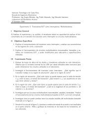
Figura <strong>2.</strong>1: Regulador proporcional inversor<br />
Si se <strong>de</strong>sea ganancia proporcional ajustable se pue<strong>de</strong> sustituir la<br />
resistencia fija R f por una resistencia variable o reóstato.<br />
Implementación <strong>de</strong> <strong>reguladores</strong> analógicos<br />
Pág.88
Rf<br />
,I<br />
8L<br />
Ro<br />
,L<br />
,P<br />
Rm<br />
-<br />
+<br />
8R<br />
Figura <strong>2.</strong>2: Regulador proporcional no inversor<br />
Rf<br />
,I<br />
8<br />
Ro1<br />
Ro2<br />
8<br />
,L<br />
,L<br />
,P<br />
Rm<br />
-<br />
+<br />
8R<br />
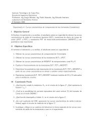
Figura <strong>2.</strong>3: Regulador proporcional diferencial<br />
Existe otra forma <strong>de</strong> obtener ganancia proporcional variable y ajustable.<br />
El procedimiento se emplea por lo general únicamente con amplificadores<br />
inversores. Como se muestra en la figura <strong>2.</strong>4, se dispone un potenciómetro en<br />
paralelo con la salida <strong>de</strong>l operacional y la referencia, y se toma la<br />
realimentación <strong>de</strong>l cursor <strong>de</strong>l potenciómetro. Si llamamos α a la relación <strong>de</strong><br />
tensiones ajustada por el potenciómetro, po<strong>de</strong>mos escribir la ganancia<br />
proporcional como:<br />
.<br />
1<br />
5<br />
I<br />
= −<br />
(<strong>2.</strong>4)<br />
α 52<br />
Implementación <strong>de</strong> <strong>reguladores</strong> analógicos<br />
Pág.89
Rf<br />
Ro<br />
-<br />
+<br />
8L<br />
Rm<br />
D8R<br />
Rq<br />
8R<br />
Figura <strong>2.</strong>4: Regulador inversor proporcional <strong>de</strong> ganancia ajustable<br />
La ganancia aumenta al disminuir la relación α, por ello, para evitar<br />
ganancias excesivas se coloca una resistencia entre el potenciómetro y<br />
referencia. A<strong>de</strong>más cuando la resistencia <strong>de</strong> realimentación R f es igual o<br />
menor que la resistencia R q <strong>de</strong>l potenciómetro se hace necesario incorporar un<br />
factor <strong>de</strong> corrección.<br />
El factor <strong>de</strong> corrección es máximo para α = 0.5, sin embargo sólo tiene<br />
importancia para los casos en los que la resistencia <strong>de</strong> realimentación R f es<br />
igual o menor que la resistencia R q <strong>de</strong>l potenciómetro.<br />
5 ⎡ 5<br />
I<br />
. = −<br />
1 ⎢1<br />
+ ( α −α<br />
2 )<br />
α 52<br />
⎢⎣<br />
5<br />
<br />
(OUHJXODGRUGHDFFLyQLQWHJUDO<br />
T<br />
I<br />
⎤<br />
⎥<br />
⎥⎦<br />
(<strong>2.</strong>5)<br />
El montaje inversor es el más usado para este tipo <strong>de</strong> regulador, tiene una<br />
función <strong>de</strong> transferencia dada por la siguiente ecuación:<br />
.<br />
,<br />
1 1 1<br />
( V)<br />
= = = .<br />
V5 & V7<br />
,<br />
V<br />
2<br />
I<br />
,<br />
(<strong>2.</strong>6)<br />
Implementación <strong>de</strong> <strong>reguladores</strong> analógicos<br />
Pág.90
Cf<br />
,I<br />
,L<br />
Ro<br />
-<br />
+<br />
8L<br />
,P<br />
Rm<br />
8R<br />
Figura <strong>2.</strong>5: Regulador inversor <strong>de</strong> acción integral<br />
Si se <strong>de</strong>sea variar la constante <strong>de</strong> tiempo <strong>de</strong> acción integral, esto pue<strong>de</strong><br />
hacerse <strong>de</strong> la misma forma que para el regulador proporcional, simplemente<br />
colocando un potenciómetro en <strong>de</strong>rivación con la salida <strong>de</strong>l amplificador<br />
operacional.<br />
Cf<br />
Ro<br />
-<br />
+<br />
8L<br />
Rm<br />
D8R<br />
Rq<br />
8R<br />
Figura <strong>2.</strong>6: Regulador inversor <strong>de</strong> acción integral con constante ajustable<br />
Tomando en cuenta el factor <strong>de</strong> corrección, la función <strong>de</strong> transferencia<br />
viene dada por:<br />
2<br />
[ 1+<br />
( α −α<br />
V5 ]<br />
1<br />
. )<br />
Vα5<br />
&<br />
( V)<br />
=<br />
&<br />
, T I<br />
2<br />
I<br />
(<strong>2.</strong>7)<br />
Implementación <strong>de</strong> <strong>reguladores</strong> analógicos<br />
Pág.91
El factor <strong>de</strong> corrección expresado entre paréntesis rectangulares<br />
correspon<strong>de</strong> a una componente <strong>de</strong> acción <strong>de</strong>rivada, con un tiempo <strong>de</strong> acción<br />
<strong>de</strong>rivada dado por:<br />
2<br />
[(<br />
α ]<br />
α − )5 T<br />
& I<br />
(<strong>2.</strong>8)<br />
Para que esto no cause problemas <strong>de</strong>be cumplirse que: la resistencia R q<br />
<strong>de</strong>l potenciómetro <strong>de</strong>be ser pequeña comparada con la resistencia <strong>de</strong> entrada<br />
R O .<br />
De todas formas, el controlador <strong>de</strong> acción integral sencillo no se utiliza<br />
muy a menudo. El montaje con acción integral variable se emplea aún con<br />
menos frecuencia como controlador in<strong>de</strong>pendiente.<br />
(OFRQWURODGRU3,<br />
Rf<br />
Cf<br />
Ro<br />
-<br />
+<br />
8L<br />
Rm<br />
8R<br />
Figura <strong>2.</strong>7: Regulador inversor <strong>de</strong> acción proporcional integral<br />
Este tipo <strong>de</strong> controlador se utiliza con mucha frecuencia en los<br />
accionamientos y en el campo <strong>de</strong> la energía eléctrica.<br />
Consi<strong>de</strong>remos primero el montaje con amplificador inversor mostrado<br />
en la figura <strong>2.</strong>7 y cuya función <strong>de</strong> transferencia está dada por la ecuación <strong>2.</strong>9.<br />
.<br />
3,<br />
⎛ ⎞<br />
⎜<br />
1<br />
V ⎟ ⎛ 1 ⎞<br />
+<br />
V<br />
5 V5 &<br />
5 &<br />
⎜ +<br />
I I<br />
7<br />
⎟<br />
⎛ 1+<br />
⎞<br />
I<br />
I I<br />
,<br />
( V)<br />
= − ⎜ ⎟ = .<br />
⎝ ⎠<br />
= .<br />
⎝ ⎠ (<strong>2.</strong>9)<br />
3<br />
3<br />
5<br />
V5 &<br />
V<br />
V<br />
2 ⎝ I I ⎠<br />
Implementación <strong>de</strong> <strong>reguladores</strong> analógicos<br />
Pág.92
Si interesa po<strong>de</strong>r ajustar la ganancia proporcional <strong>de</strong>l controlador PI<br />
mediante un potenciómetro, <strong>de</strong>be emplearse el montaje <strong>de</strong> la figura <strong>2.</strong>8 en<br />
don<strong>de</strong> la ganancia proporcional ajustable K Pα y el tiempo <strong>de</strong> acción integral<br />
ajustable T Iβ se calculan <strong>de</strong> la siguiente forma:<br />
5 ⎡ 5 ⎤<br />
I<br />
T<br />
. = −<br />
1 ⎢1<br />
+ ( −<br />
2<br />
3α α α ) ⎥<br />
(<strong>2.</strong>10)<br />
5 α<br />
2 ⎢⎣<br />
5<br />
I ⎥⎦<br />
5 ⎡<br />
⎤<br />
I<br />
⋅ β5<br />
S<br />
5<br />
2 T<br />
β<br />
=<br />
I ⎢1<br />
+ ( α −α<br />
) ⎥<br />
(<strong>2.</strong>11)<br />
5<br />
I<br />
+ β5<br />
S ⎢⎣<br />
5<br />
I ⎥⎦<br />
,<br />
Rf<br />
Cf<br />
Ro<br />
-<br />
+<br />
8L<br />
Rm<br />
E5S<br />
Rp<br />
D8R<br />
Rq<br />
8R<br />
Figura <strong>2.</strong>8: Regulador inversor <strong>de</strong> acción proporcional integral ajustable<br />
El reóstato R P <strong>de</strong>be tener una relación <strong>de</strong> división β comprendida entre<br />
0.01 y 1. Si la resistencia fija <strong>de</strong>l reóstato R p es aproximadamente 0.1 R f y su<br />
resistencia global máxima <strong>de</strong> 10 R f , el tiempo <strong>de</strong> acción integral T Iβ pue<strong>de</strong><br />
ajustarse en la relación 1 a 10. Los ajustes son casi in<strong>de</strong>pendientes y un ajuste<br />
erróneo <strong>de</strong> la ganancia proporcional se corrige mediante una variación <strong>de</strong> la<br />
relación <strong>de</strong> división α y un ajuste erróneo <strong>de</strong>l tiempo <strong>de</strong> acción integral,<br />
<strong>de</strong>bido a la influencia <strong>de</strong>l ajuste <strong>de</strong> la ganancia proporcional K pα , se elimina<br />
con una pequeña modificación <strong>de</strong> la relación <strong>de</strong> división β.<br />
<br />
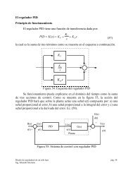
(OFRPSHQVDGRUGHDGHODQWR3'<br />
Realizado con un operacional inversor, el compensador <strong>de</strong> a<strong>de</strong>lanto o<br />
PD tiene la función <strong>de</strong> transferencia dada en la ecuación <strong>2.</strong>1<strong>2.</strong><br />
Implementación <strong>de</strong> <strong>reguladores</strong> analógicos<br />
Pág.93
Rf1<br />
Rf2<br />
Ro<br />
-<br />
+<br />
Cq<br />
8L<br />
Rm<br />
Rd<br />
8R<br />
Figura <strong>2.</strong>9: Regulador inversor <strong>de</strong> acción proporcional <strong>de</strong>rivada o PD<br />
.<br />
3'<br />
5<br />
( V)<br />
= −<br />
⎛<br />
⎜<br />
5<br />
⋅ 5<br />
⎞<br />
⎟<br />
I 1 I 2<br />
1+<br />
V + 5G<br />
&<br />
T<br />
I<br />
5 ⎜ 5<br />
I<br />
I<br />
5 ⎟<br />
⎝ +<br />
1<br />
+<br />
2<br />
1 I 2 ⎠ 1+<br />
V(<br />
'<br />
+ WG<br />
)<br />
= −.<br />
(<strong>2.</strong>12)<br />
3<br />
52<br />
1+<br />
V5G&<br />
T<br />
1+<br />
VWG<br />
La resistencia <strong>de</strong> amortiguamiento R d evita la entrada en oscilación <strong>de</strong>l<br />
circuito y da lugar a la constante <strong>de</strong> tiempo parásita t d .<br />
Si se <strong>de</strong>sea un regulador PD ajustable, se pue<strong>de</strong> usar el circuito usado en<br />
el regulador PID ajustable mostrado en la figura <strong>2.</strong>11. El regulador PD<br />
ajustable correspon<strong>de</strong> al circuito más a la <strong>de</strong>recha en esa figura y es un<br />
circuito no inversor con ganancia proporcional igual a uno. La función <strong>de</strong><br />
transferencia para este regulador se muestra en la ecuación <strong>2.</strong>13.<br />
(OUHJXODGRU3,'<br />
.<br />
3'<br />
( V)<br />
=<br />
(1 + V7<br />
(1 + VW<br />
'<br />
G<br />
γ<br />
)<br />
)<br />
(<strong>2.</strong>13)<br />
La combinación <strong>de</strong> las acciones PI y PD da lugar a la acción PID o<br />
acción proporcional, integral y <strong>de</strong>rivada.<br />
.<br />
3,'<br />
( V)<br />
= −<br />
[ 1+<br />
V(<br />
5 + 5 )&<br />
]<br />
I<br />
1<br />
I<br />
V5<br />
2<br />
2<br />
&<br />
I<br />
⎡ 5<br />
I<br />
⋅ 1<br />
I ⎢ + V<br />
⎢⎣<br />
5<br />
I<br />
(1 + V5 & )<br />
G<br />
T<br />
1<br />
1<br />
⋅ 5<br />
I<br />
+ 5<br />
I<br />
2<br />
2<br />
&<br />
T<br />
⎤<br />
⎥<br />
⎥⎦<br />
(<strong>2.</strong>14)<br />
Implementación <strong>de</strong> <strong>reguladores</strong> analógicos<br />
Pág.94
Empleando un amplificador inversor se obtiene el PID mostrado en la<br />
figura <strong>2.</strong>10; po<strong>de</strong>mos escribir la función <strong>de</strong> transferencia siguiente para el<br />
circuito PID:<br />
Rf1<br />
Cf<br />
Rf2<br />
Ro<br />
-<br />
+<br />
Cq<br />
8L<br />
Rm<br />
Rd<br />
8R<br />
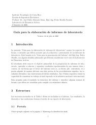
Figura <strong>2.</strong>10: Regulador inversor <strong>de</strong> acción PID<br />
Existen a<strong>de</strong>más circuitos como <strong>de</strong>l <strong>de</strong> la figura <strong>2.</strong>11 que permiten variar<br />
todos los parámetros <strong>de</strong>l PID y está formado por tres amplificadores<br />
operacionales. La función <strong>de</strong> transferencia <strong>de</strong> este circuito se encuentra en la<br />
ecuación <strong>2.</strong>15 con los parámetros dados por las ecuaciones siguientes:<br />
7<br />
5<br />
1 ⎡<br />
5 ⎤<br />
2 T<br />
⋅ ⎢1<br />
+ ( α −α<br />
) ⎥<br />
α ⎢⎣<br />
5<br />
I 1 ⎥⎦<br />
⋅ 53<br />
50<br />
& 7 = α ⋅ β ⋅ ⋅ 5 ⋅<br />
P<br />
P<br />
+ 5<br />
5<br />
I 1<br />
3α =<br />
, β<br />
= β ⋅ ⋅ &<br />
P I<br />
50<br />
5<br />
I 2<br />
= γ<br />
&<br />
' γ ,<br />
γ ⋅ 5<br />
I<br />
I<br />
I 1<br />
2<br />
.<br />
3,'<br />
3<br />
( V)<br />
= −.<br />
3<br />
= ε ⋅7<br />
G<br />
αβ ' γ<br />
[ 1+<br />
V7 ] ⋅[ 1+<br />
V7 ]<br />
α (<strong>2.</strong>15)<br />
V7 (1 + VW )<br />
,<br />
,<br />
β<br />
αβ<br />
G<br />
'<br />
γ<br />
Cf<br />
Rf1<br />
J 5I<br />
Ro<br />
-<br />
+<br />
8<br />
R1<br />
-<br />
+<br />
8<br />
H 5<br />
H 5<br />
8L<br />
Rm1<br />
D8<br />
Rq<br />
5P<br />
R2<br />
Cm<br />
-<br />
+<br />
8R<br />
Figura <strong>2.</strong>11: Regulador PID ajustable<br />
Implementación <strong>de</strong> <strong>reguladores</strong> analógicos<br />
Pág.95